OPEN-SOURCE SCRIPT
Trig-Log Scaled Momentum Oscillator
Taylor Series Approximations for Trigonometry:
1. The indicator starts by calculating sine and cosine values of the close price using Taylor Series approximations. These approximations use polynomial terms to estimate the values of these trigonometric functions.
Mathematical Component Formation:
2. The calculated sine and cosine values are then multiplied together. This gives us the primary mathematical component, termed as the 'trigComponent'.
Smoothing Process:
3. To ensure that our indicator is less susceptible to market noise and more reactive to genuine price movements, this 'trigComponent' undergoes a smoothing process using a simple moving average (SMA). The length of this SMA is defined by the user.
Logarithmic Transformation:
4. With our smoothed value, we apply a natural logarithm approximation. Again, this approximation is based on the Taylor expansion. This step ensures that all resultant values are positive and offers a different scale to interpret the smoothed component.
Dynamic Scaling:
5. To make our indicator more readable and comparable over different periods, the logarithmically transformed values are scaled between a range. This range is determined by the highest and lowest values of the transformed component over the user-defined 'lookback' period.
ROC (Rate of Change) Direction:
6. The direction of change in our scaled value is determined. This offers a quick insight into whether our mathematical component is increasing or decreasing compared to the previous value.
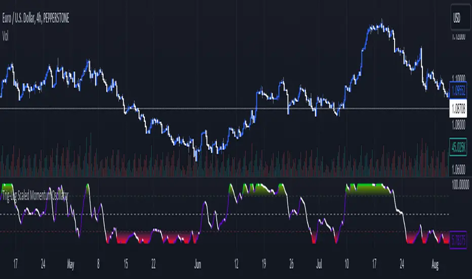
Visualization:
7. Finally, the indicator plots the dynamically scaled and smoothed mathematical component on the chart. The color of the plotted line depends on its direction (increasing or decreasing) and its boundary values.
1. The indicator starts by calculating sine and cosine values of the close price using Taylor Series approximations. These approximations use polynomial terms to estimate the values of these trigonometric functions.
Mathematical Component Formation:
2. The calculated sine and cosine values are then multiplied together. This gives us the primary mathematical component, termed as the 'trigComponent'.
Smoothing Process:
3. To ensure that our indicator is less susceptible to market noise and more reactive to genuine price movements, this 'trigComponent' undergoes a smoothing process using a simple moving average (SMA). The length of this SMA is defined by the user.
Logarithmic Transformation:
4. With our smoothed value, we apply a natural logarithm approximation. Again, this approximation is based on the Taylor expansion. This step ensures that all resultant values are positive and offers a different scale to interpret the smoothed component.
Dynamic Scaling:
5. To make our indicator more readable and comparable over different periods, the logarithmically transformed values are scaled between a range. This range is determined by the highest and lowest values of the transformed component over the user-defined 'lookback' period.
ROC (Rate of Change) Direction:
6. The direction of change in our scaled value is determined. This offers a quick insight into whether our mathematical component is increasing or decreasing compared to the previous value.
Visualization:
7. Finally, the indicator plots the dynamically scaled and smoothed mathematical component on the chart. The color of the plotted line depends on its direction (increasing or decreasing) and its boundary values.
開源腳本
本著TradingView的真正精神,此腳本的創建者將其開源,以便交易者可以查看和驗證其功能。向作者致敬!雖然您可以免費使用它,但請記住,重新發佈程式碼必須遵守我們的網站規則。
免責聲明
這些資訊和出版物並不意味著也不構成TradingView提供或認可的金融、投資、交易或其他類型的意見或建議。請在使用條款閱讀更多資訊。
開源腳本
本著TradingView的真正精神,此腳本的創建者將其開源,以便交易者可以查看和驗證其功能。向作者致敬!雖然您可以免費使用它,但請記住,重新發佈程式碼必須遵守我們的網站規則。
免責聲明
這些資訊和出版物並不意味著也不構成TradingView提供或認可的金融、投資、交易或其他類型的意見或建議。請在使用條款閱讀更多資訊。