Madrid

Madrid Sinewave

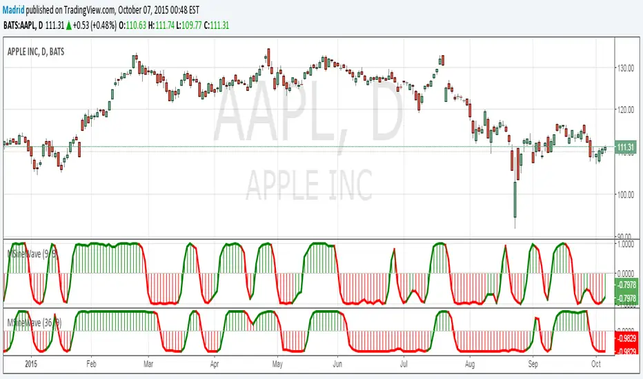
This implements the Even Better Sinewave indicator as described in the book Cycle Analysis for Traders by John F. Ehlers.
In the example I used 36 as the cycle to be analyzed and a second cycle with a shorter period, 9, the larger period tells where the dominant cycle is heading, and the faster cycle signals entry/exit points and reversals.

開源腳本

本著真正的TradingView精神,該腳本的作者將其開源發布,以便交易者可以理解和驗證它。為作者喝彩吧!您可以免費使用它,但在出版物中重複使用此代碼受網站規則的約束。 您可以收藏它以在圖表上使用。

免責聲明

這些資訊和出版物並不意味著也不構成TradingView提供或認可的金融、投資、交易或其他類型的意見或建議。請在使用條款閱讀更多資訊。

想在圖表上使用此腳本?
// Madrid : 09/Jun/2015 21:09 : Even Better Sinewave : 1.0
// This implements the Even Better Sinewave indicator 
// Ref. Cycle Analysis for Traders by John F. Ehlers.
//

study("Madrid Sinewave", shorttitle="MSineWave")
Duration = input(36)
src = close

OB = 0.85, OS = -0.85
PI = 3.14159265358979

deg2rad( deg ) =>
        deg*PI/180.0

lowerBand = input(9)
ssFilter( price, lowerBand ) =>
    angle = sqrt(2)*PI/lowerBand
    a1= exp(-angle)
    b1 = 2*a1*cos(angle)
    c2 = b1
    c3 = -a1*a1
    c1 = 1 - c2 -c3
    filt = c1*(price + nz(price[1]))/2 + c2*nz(filt[1]) + c3*nz(filt[2])


// HighPass filter cyclic components whose periods are shorter than Duration input
x = src
angle = deg2rad(360)/Duration
alpha1 = ( 1-sin(angle) ) / cos(angle)
HP = 0.5*(1+alpha1)*(x-x[1]) + alpha1*nz(HP[1],0)

// Smooth with a Super Smoother Filter
Filt = ssFilter( HP, lowerBand )

Wave = ( Filt + nz(Filt[1],0) + nz(Filt[2],0) ) / 3
Pwr = ( Filt*Filt + nz(Filt[1],0)* nz(Filt[1],0) +  nz(Filt[2],0)* nz(Filt[2],0) ) /3

// Normalize the Average Wave to Square Root of the Average Power
sineWave = Wave / sqrt(Pwr)

// Output
sineWaveColor = sineWave>OB?green
            :  sineWave<OS?red
            :  change(sineWave)>0?green
            :  red

plot( sineWave, color=sineWaveColor, linewidth=3 )
plot( sineWave, color=sineWaveColor, linewidth=1, style=histogram )

hline(0, color=silver, linestyle=dotted)