Propagation Volumes and Trends

2016年1月28日

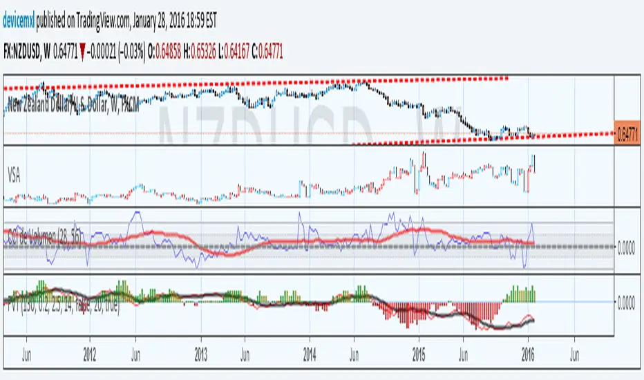
With this, i calculate RSI of the HL2 of the volume and use like an oscillator, this will use to measure the strength of the trend and the "Volume Flow" to follow the trend.

I use like foundation the LazyBear "Volume Flow Indicator" "honor a quien honor merece"

Background:
I think the volume as the price could be represented by candles or other graphic to use indicators and strengthen their analysis, due to lack of registration of this it is first necessary to calculate a volume graph, if the candle traditionally negative price brand then the total volume is taken as negative for the period. An example of this is in the On Balance Volume indicator, the problem is that there is no way to analyze the volume using other methods. An approximate volume of the spread could be the use of the price spread to make a synthetic behavior

As traditionally is observed if Open> Close then the candle and the volume will be negative and vice versa; the next step, is estimate the amounts of the candle necessary to calculate the ratio to use for the volume and thus idealize their spread within the candle:

VLOW = Volume x Low
vHigh = x High Volume
VOpen = vClose [1]
vClose = Volume x Close

This graph can show a stable synthetic form of fluctuations in the volume trend affected by price.
ideas, comments and suggestions (or corrections).They are always welcome