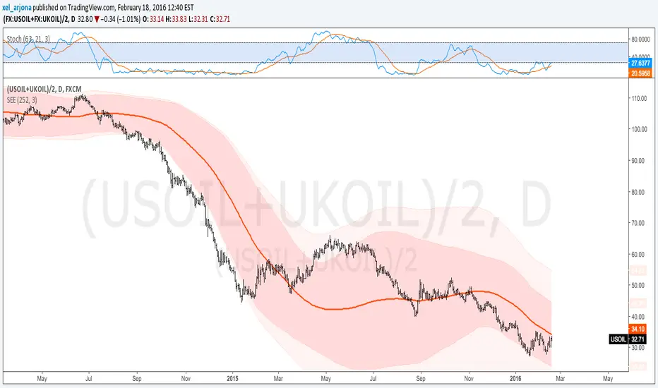
Standard Error of the Estimate -Composite Bands-

Standard Error of the Estimate - Code and adaptation by glaz & xel_arjona
Ver. 2.00.a

Original implementation idea of bands by:
Traders issue: Stocks & Commodities V. 14:9 (375-379):
Standard Error Bands by Jon Andersen

This code is a former update to previous "Standard Error Bands" that was wrongly applied given that previous version in reality use the Standard Error OF THE MEAN, not THE ESTIMATE as it should be used by Jon Andersen original idea and corrected in this version.

As always I am very Thankfully with the support at the Pine Script Editor chat room, with special mention to user glaz in order to help me adequate the alpha-beta (y-y') algorithm, as well to give him full credit to implement the "wide" version of the former bands.

For a quick and publicly open explanation of this truly statistical (regression analysis) indicator, you can refer at Here!

Extract from the former URL:
Standard Error Bands are quite different than Bollinger's. First, they are bands constructed around a linear regression curve. Second, the bands are based on two standard errors above and below this regression line. The error bands measure the standard error of the estimate around the linear regression line. Therefore, as a price series follows the course of the regression line the bands will narrow, showing little error in the estimate. As the market gets noisy and random, the error will be greater resulting in wider bands.