Digitalsignalprocessing — 指標和策略

Ehlers Adaptive Trend Indicator [Alpha Extract]Ehlers Adaptive Trend Indicator The Ehlers Adaptive Trend Indicator combines Ehlers' advanced digital signal processing techniques with dynamic volatility bands to identify robust trend conditions and potential reversals. This powerful tool helps traders visualize trend strength, adaptive support/resistance levels, and momentum shifts across various market conditions. 🔶 CALCULATION The indicator employs a sophisticated adaptive algorithm that responds to changing market conditions: • Ehlers Filter : Calculates a weighted average based on momentum differences to create an adaptive trend baseline. • Dynamic Bands : Volatility-adjusted bands that expand and contract based on recent price action. • Trend Level : A dynamic support/resistance level that adapts to the current trend direction. • Smoothed Volatility : Market volatility measured and smoothed to provide reliable band width. Formula: • Ehlers Basis = Weighted average of price, with weights determined by momentum differences • Volatility = Standard deviation of price over Ehlers Length period • Smoothed Volatility = EMA of volatility over Smoothing Length • Upper Band = Ehlers Basis + Smoothed Volatility × Sensitivity • Lower Band = Ehlers Basis - Smoothed Volatility × Sensitivity • Trend Level = Adaptive support in uptrends, resistance in downtrends 🔶 DETAILS 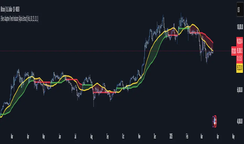Visual Features : • Ehlers Basis Line (Yellow): The core adaptive trend reference that serves as the primary trend indicator. • Trend Level Line (Dynamic Color): Changes between green (bullish) and red (bearish) based on the current trend state. • Fill Areas : Transparent green fill during bullish trends and transparent red fill during bearish trends for clear visual identification. • Bar Coloring : Optional price bar coloring that reflects the current trend direction for enhanced visualization. Interpretation : • **Bullish Signal**: Price crosses above the upper band, triggering a trend change with the Trend Level becoming dynamic support. • **Bearish Signal**: Price drops below the lower band, confirming a trend change with the Trend Level becoming dynamic resistance. • **Trend Continuation**: Trend Level rises in bullish markets and falls in bearish markets, providing adaptive trailing support/resistance. 🔶 EXAMPLES The chart demonstrates: • Bullish Trend Identification : When price breaks above the upper band, the indicator shifts to bullish mode with green trend level and fill. • Bearish Trend Identification : When price falls below the lower band, the indicator shifts to bearish mode with red trend level and fill. • Trend Persistence : Trend Level adapts to market movement, rising during uptrends to provide dynamic support and falling during downtrends to act as resistance. Example Snapshots : • During a strong uptrend, the Trend Level continuously adjusts upward, keeping traders in the trend while filtering out minor retracements. • During trend reversals, clear color changes and Trend Level shifts provide early warning of potential direction changes. 🔶 SETTINGS Customization Options : • Ehlers Length (p1) (Default: 30): Controls the primary adaptive calculation period, balancing responsiveness with stability. • Momentum Length (p2) (Default: 25): Determines the lag for momentum calculations used in the adaptive weighting. • Smoothing Length (Default: 10): Adjusts the volatility smoothing period—higher values provide more stable bands. • Sensitivity (Default: 1.0): Multiplier for band width—higher values increase distance between bands, lower values tighten them. • Visual Settings : Customizable colors for bullish and bearish trends, basis line, and optional bar coloring. The Ehlers Adaptive Trend Indicator combines John Ehlers' digital signal processing expertise with modern volatility analysis to create a robust trend-following system that adapts to changing market conditions, helping traders stay on the right side of the market.

[GYTS] Ultimate Smoother (3-poles + 2 poles)Ultimate Smoother (3-pole) 🌸 Part of GoemonYae Trading System (GYTS) 🌸 🌸 --------- INTRODUCTION --------- 🌸 💮 Release of 3-Pole Ultimate Smoother This indicator presents a new 3-pole version of John Ehlers' Ultimate Smoother (2024) . This results in an unconventional filter that exhibits effectively zero lag in practical trading applications, regardless of the set period. By using a 2-pole high-pass filter in its design, it responds to price direction changes on the same bar, while still allowing the user to control smoothness. 💮 What is the Ultimate Smoother? The original Ultimate Smoother is a revolutionary filter designed by John Ehlers (2024) that smooths price data with virtually zero lag in the pass band. While conventional filters always introduce lag when removing market noise, the Ultimate Smoother maintains phase alignment at low frequencies while still providing excellent noise reduction. 💮 Mathematical Foundation The Ultimate Smoother achieves its remarkable properties through a clever mathematical approach: 1. Instead of directly designing a low-pass filter (like traditional moving averages), it subtracts a high-pass filter from an all-pass filter (the original input data). 2. At very low frequencies, the high-pass filter contributes almost nothing, so the output closely matches the input in both amplitude and phase. 3. At higher frequencies, the high-pass filter's response increasingly matches the input data, resulting in cancellation through subtraction. The 3-pole version extends this principle by using a higher-order high-pass filter, requiring additional coefficients and handling more terms in the numerator of the transfer function. 🌸 --------- USAGE GUIDE --------- 🌸 💮 Period Parameter Behaviour The period parameter in the 3-pole Ultimate Smoother works somewhat counterintuitively: - Longer periods: Result in less smooth, but more responsive following of the price. The filter output more closely tracks the input data. - Shorter periods: Produce smoother output but may exhibit overshooting (extrapolating price movement) for larger movements. This is different from most filters where longer periods typically produce smoother outputs with more lag. 💮 When to Choose 3-Pole vs. 2-Pole - Choose the 3-pole version when you need zero-lag but want to control the smoothness - Choose the 2-pole version when you are okay with some lag with the benefit of more smoothness. 🌸 --------- ACKNOWLEDGEMENTS --------- 🌸 This indicator builds upon the pioneering work of John Ehlers, particularly from his article April 2024 edition of TASC's Traders' Tips . The original version is published on TradingView by @PineCodersTASC . This 3-pole extension was developed by @GoemonYae . Feedback is highly appreciated!

Reflex & Trendflex █ OVERVIEW Reflex and Trendflex are zero-lag oscillators that decompose price into independent cycle and trend components using SuperSmoother filtering. These indicators isolate each component separately, providing clearer identification of cyclical reversals (Reflex) versus trending movements (Trendflex). Based on Dr. John F. Ehlers' "Reflex: A New Zero-Lag Indicator" article (February 2020, TASC), both oscillators use normalized slope deviation analysis to minimize lag while maintaining signal clarity. The SuperSmoother filter removes high-frequency noise, then deviations from linear regression (Reflex) or current value (Trendflex) are measured and normalized by RMS for consistent amplitude across instruments and timeframes. █ CONCEPTS SuperSmoother Filter Both oscillators begin with a two-pole Butterworth low-pass filter that smooths price data without the excessive lag of simple moving averages. The filter uses exponential decay coefficients and cosine modulation based on the cutoff period, providing aggressive smoothing while preserving signal timing. Reflex: Cycle Component Reflex isolates cyclical price behavior by measuring deviation from a linear regression line fitted through the SuperSmoother output. For each bar, the filter calculates a linear slope over the lookback period, then sums how much the smoothed price deviates from this trendline. These deviations represent pure cyclical movement - price oscillations around the dominant trend. The result is normalized by RMS (root mean square) to produce consistent amplitude regardless of volatility or timeframe. Trendflex: Trend Component Trendflex extracts trending behavior by measuring cumulative deviation from the current SuperSmoother value. Instead of comparing to a regression line, it simply sums the differences between the current smoothed value and all past values in the period. This captures sustained directional movement rather than oscillations. Like Reflex, normalization by RMS ensures comparable readings across different instruments. RMS Normalization Both oscillators normalize their raw deviation measurements using an exponentially weighted RMS calculation: `rms = 0.04 * deviation² + 0.96 * rms `. This adaptive normalization ensures the oscillator amplitude remains stable as volatility changes, making threshold levels meaningful across different market conditions. █ INTERPRETATION Reflex (Cycle Component) Oscillates around zero representing cyclical price behavior isolated from trend: • Above zero : Price is in upward phase of cycle • Below zero : Price is in downward phase of cycle • Zero crossings : Potential cycle reversal points • Extremes : Indicate stretched cyclical condition, often precede mean reversion Best used for identifying cyclical turning points in ranging or oscillating markets. More sensitive to reversals than Trendflex. Trendflex (Trend Component) Oscillates around zero representing trending behavior isolated from cycles: • Above zero : Sustained upward trend • Below zero : Sustained downward trend • Zero crossings : Trend direction changes • Magnitude : Strength of trend (larger absolute values = stronger trend) Best used for confirming trend direction and identifying trend exhaustion. Less noisy than Reflex due to focus on directional movement rather than oscillations. Combined Analysis Using both oscillators together provides powerful signal confirmation: • Both positive: Strong uptrend with positive cycle phase (high probability long setup) • Both negative: Strong downtrend with negative cycle phase (high probability short setup) • Divergent signals: Conflicting cycle and trend (choppy conditions, reduce position size) • Reflex reversal with Trendflex agreement: Cyclical turn within established trend (entry/exit timing) Dynamic Thresholds Threshold bands identify statistically significant oscillator readings that warrant attention: • Breach above +threshold : Strong bullish cycle (Reflex) or trend (Trendflex) behavior - potential overbought condition • Breach below -threshold : Strong bearish cycle or trend behavior - potential oversold condition • Return inside thresholds : Signal strength normalizing, potential reversal or consolidation ahead • Threshold compression : During low volatility, thresholds narrow (especially with StdDev mode), making breaches more frequent • Threshold expansion : During high volatility, thresholds widen, filtering out minor oscillations Combine threshold breaches with zero-line position for stronger signals: • Threshold breach + zero-line cross = high-conviction signal • Threshold breach without zero-line support = monitor for confirmation Alert Conditions Six built-in alerts trigger on bar close (no repainting): • Above +Threshold : Oscillator crossed above positive threshold (strong bullish behavior) • Below -Threshold : Oscillator crossed below negative threshold (strong bearish behavior) • Reflex Above Zero : Reflex crossed above zero (bullish cycle phase) • Reflex Below Zero : Reflex crossed below zero (bearish cycle phase) • Trendflex Above Zero : Trendflex crossed above zero (bullish trend shift) • Trendflex Below Zero : Trendflex crossed below zero (bearish trend shift) █ SETTINGS & PARAMETER TUNING Oscillator Settings • Source : Price series to decompose • Reflex Period (5-50): SuperSmoother period for cycle component. Lower values increase responsiveness to cyclical turns but add noise. Default 20. • Trendflex Period (5-50): SuperSmoother period for trend component. Lower values respond faster to trend changes. Default 20. Display Settings • Reflex/Trendflex Display : Toggle visibility and customize colors for each oscillator independently • Zero Line : Reference line showing neutral oscillator position Dynamic Thresholds Optional significance bands that identify when oscillator readings indicate strong cyclical or trending behavior: • Threshold Mode : Choose calculation method based on market characteristics - MAD (Median Absolute Deviation) : Outlier-resistant, best for markets with occasional spikes (default) - Standard Deviation : Volatility-sensitive, adapts quickly to regime changes - Percentile Rank : Fixed probability bands (e.g., 90% = only 10% of values exceed threshold) • Apply To : Select which oscillator (Reflex or Trendflex) to calculate thresholds for • Period (2-200): Lookback window for threshold calculation. Default 50. • Multiplier (k) : Scaling factor for MAD/StdDev modes. Higher values = fewer threshold breaches (default 1.5) • Percentile (%) : For Percentile mode only. Higher percentile = more selective threshold (default 90%) Parameter Interactions • Shorter periods make both oscillators more sensitive but noisier • Reflex typically more volatile than Trendflex at same period settings • For ranging markets: shorter Reflex period (10-15) captures swings better • For trending markets: shorter Trendflex period (10-15) follows trend shifts faster █ LIMITATIONS Inherent Characteristics • Near-zero lag, not zero-lag : Despite the name, some lag remains from SuperSmoother filtering • Normalization artifacts : RMS normalization can produce unusual readings during volatility regime changes • Period dependency : Oscillator characteristics change significantly with different period settings - no "correct" universal parameter Market Conditions to Avoid • Very low volatility : Normalization amplifies noise in quiet markets, producing false signals • Sudden gaps : SuperSmoother assumes continuous data; large gaps disrupt filter continuity requiring bars to stabilize • Micro timeframes : Sub-minute charts contain microstructure noise that overwhelms signal quality Parameter Selection Pitfalls • Matching periods to dominant cycle : If period doesn't align with actual market cycle period, signals degrade • Threshold over-tuning : Optimizing threshold parameters for past data often fails forward - use conservative defaults • Ignoring component differences : Reflex and Trendflex measure different aspects - don't expect identical behavior █ NOTES Credits These indicators are based on Dr. John F. Ehlers' "Reflex: A New Zero-Lag Indicator" published in the February 2020 issue of Technical Analysis of Stocks & Commodities (TASC) magazine. The article introduces a novel approach to isolating cycle and trend components using SuperSmoother filtering combined with normalized deviation analysis. For those interested in the underlying mathematics and DSP concepts: • Ehlers, J.F. (February 2020). "Reflex: A New Zero-Lag Indicator" - Technical Analysis of Stocks & Commodities magazine • Ehlers, J.F. (2001). Rocket Science for Traders: Digital Signal Processing Applications . John Wiley & Sons • Various TASC articles by John Ehlers on SuperSmoother filters and oscillator design by ♚@e2e4

Fourier series Model Of The Market █ OVERVIEW The Fourier Series Model of the Market (FSMM) decomposes price action into harmonic components using bandpass filtering, then reconstructs a composite wave weighted by rolling energy ratios. This approach isolates cyclical market behavior at multiple frequencies, emphasizing dominant cycles for cleaner signal generation. The energy-adaptive weighting is the key differentiator from simple harmonic summation: cycles that dominate current price action contribute more to the output. Based on Fourier analysis principles applied to financial markets, the indicator extracts harmonics (fundamental, 2nd, 3rd, etc.) using second-order IIR bandpass filters, then weights each harmonic's contribution by its relative energy compared to adjacent harmonics. This energy-adaptive weighting naturally emphasizes the cycles that are most prominent in current market conditions. █ CONCEPTS Fourier Decomposition Fourier analysis represents any periodic signal as a sum of sine waves at different frequencies. In market analysis, price action can be decomposed into a fundamental cycle (the base period) plus harmonics at integer multiples of that frequency (period/2, period/3, etc.). Each harmonic captures oscillations at a specific frequency band, and their sum reconstructs the original cyclical behavior. Bandpass Filtering Each harmonic is extracted using a second-order IIR (Infinite Impulse Response) bandpass filter tuned to that harmonic's frequency. The filter isolates price activity within a narrow frequency range while rejecting both higher-frequency noise and lower-frequency trend drift. Before filtering, the source is debiased via 2-bar momentum to remove DC offset, ensuring each bandpass operates around true zero. Energy-Weighted Reconstruction Rather than simply summing all harmonics equally, FSMM weights each harmonic by its rolling energy relative to the previous harmonic. The energy score combines the current harmonic value with its rate of change, so it reflects both amplitude and momentum. Higher harmonics that hold comparatively more energy therefore contribute more to the composite wave, while weaker harmonics fade out. This adaptive weighting allows the model to respond to changing market cyclicality. Quadrature Component (Rate of Change) The rate of change output represents the 90°-phase-shifted (quadrature) component of the wave. When the wave is at zero and rising, the rate of change is at maximum positive. This provides complementary information about cycle phase and can be used for timing entries relative to cycle position. █ INTERPRETATION Wave Output The composite wave oscillates around zero, representing the sum of all extracted harmonic components weighted by energy: • Above zero : Net bullish cyclical momentum across harmonics • Below zero : Net bearish cyclical momentum across harmonics • Zero crossings : Cycle phase transitions - potential reversal points • Wave amplitude : Strength of cyclical behavior; larger swings indicate cleaner cycles Rate of Change The quadrature component (90° phase-shifted) provides cycle phase information: • Maximum rate of change : Wave is near zero and accelerating - early cycle phase • Zero rate of change : Wave is at peak or trough - cycle extremes • Rate/Wave divergence : When wave makes new highs/lows but rate of change does not confirm (lower momentum), suggests cycle exhaustion or impending phase shift Combined Analysis • Wave crossing above zero with positive rate of change: Strong bullish cycle initiation • Wave crossing below zero with negative rate of change: Strong bearish cycle initiation • Wave at extreme with rate of change reversing: Potential cycle peak/trough Threshold Bands When enabled, threshold bands define statistically significant wave deviations: • Breach above +threshold : Unusually strong bullish cyclical behavior • Breach below -threshold : Unusually strong bearish cyclical behavior • Return inside thresholds : Normalizing behavior, potential mean reversion ahead Alert Conditions Four built-in alerts trigger on bar close (no repainting): • Above +Threshold : Strong bullish cycle behavior • Below -Threshold : Strong bearish cycle behavior • Above Zero : Bullish cycle phase shift • Below Zero : Bearish cycle phase shift █ SETTINGS & PARAMETER TUNING Fourier Series Model • Source : Price series to decompose into harmonic components. • Period (6-100): Base period for the fundamental harmonic. Higher harmonics divide this period (harmonic 2 = period/2, harmonic 3 = period/3). Match to the dominant market cycle for best results. Default 20. • Bandwidth (0.05-0.5): Bandpass filter selectivity. Lower values create narrower passbands that isolate harmonics more precisely but may miss slightly off-frequency cycles. Higher values capture broader ranges but reduce harmonic separation. Default 0.1 balances precision and robustness. • Harmonics (1-20): Number of harmonic components to extract. More harmonics capture finer cyclical detail but increase computation. For most applications, 3-5 harmonics suffice. The fundamental alone (1 harmonic) functions as a simple bandpass filter. Display Settings • Wave Outputs : Toggle visibility and color of the composite Fourier wave. • Rate of Change : Toggle visibility and color of the quadrature component (90° phase-shifted wave). • Zero Line : Reference line for oscillator neutrality. Diagnostics - Dynamic Thresholds Optional significance bands that identify when wave readings indicate strong cyclical behavior: • Dynamic Threshold : Toggle threshold bands and set colors. • Threshold Mode : Select calculation method: - MAD (Median Absolute Deviation) : Robust, outlier-resistant measure using k * MAD where MAD ≈ 0.6745 * stdev. - Standard Deviation : Volatility-sensitive, calculated as k * stdev of wave over the lookback period. - Percentile Rank : Fixed probability bands using percentile of |wave| (90% means only 10% of values exceed threshold). • Period (2-200): Lookback for threshold calculations. Default 50. • Multiplier (k) : Scaling for MAD/Standard Deviation modes. Default 1.5. • Percentile (%) (0-100): For Percentile Rank mode only. Default 90%. Parameter Interactions • Shorter periods respond faster to cycle changes but may capture noise. • Lower bandwidth + more harmonics = more precise decomposition but requires accurate period setting. • Higher bandwidth is more forgiving of period mismatches. • For strongly trending markets, restrict harmonics to 1-2 so the model tracks the dominant cycle with fewer higher-frequency components. • For ranging/oscillating markets, more harmonics (4-6) capture complex cycles. █ LIMITATIONS Inherent Characteristics • Period dependency : Effectiveness depends on correctly matching the Period parameter to actual market cycles. Use cycle measurement tools (autocorrelation, FFT, dominant cycle indicators) to identify appropriate periods. • Stationarity assumption : The indicator assumes cycle frequencies remain relatively stable within the lookback window. Rapidly shifting dominant cycles (regime transitions) may produce inconsistent results until the buffer adapts. • Filter lag : Despite bandpass design, some lag remains inherent to causal filtering. Higher harmonics have less lag but more noise sensitivity. • Energy weighting artifacts : During regime changes when harmonic energy ratios shift rapidly, weighting may produce transient anomalies. Market Conditions to Avoid • Strong trending markets : Pure trends with no cyclicality produce weak, meandering signals. The indicator assumes cyclical market behavior. • News events/gaps : Large discontinuities disrupt filter continuity. Requires 1-2 full periods to stabilize. • Period mismatch : If the Period parameter doesn't match actual market cycles, harmonic extraction produces noise rather than signal. Parameter Selection Pitfalls • Too many harmonics : Beyond 5-6 harmonics, additional components often capture noise rather than meaningful cycles. • Bandwidth too narrow : Very low bandwidth (< 0.05) requires extremely precise period matching; slight mismatches cause signal loss. • Over-optimization : Perfect historical parameter fits typically fail forward. Use robust defaults across multiple instruments. █ NOTES Credits This indicator applies Fourier analysis principles to financial market data, building on the extensive work of Dr. John F. Ehlers in applying digital signal processing to trading. The bandpass filter implementation and harmonic decomposition approach draw from DSP fundamentals as presented in Ehlers' publications. For those interested in the underlying mathematics and DSP concepts: • Ehlers, J.F. (2001). Rocket Science for Traders: Digital Signal Processing Applications . John Wiley & Sons. • Ehlers, J.F. (2013). Cycle Analytics for Traders . John Wiley & Sons. • Various TASC articles by John Ehlers on bandpass filters, cycle analysis, and harmonic decomposition. by ♚@e2e4

Voss Predictive Filter █ OVERVIEW The Voss Predictive Filter (VPF) is a negative group delay (NGD) filter that anticipates cyclical price movement through phase compensation. The VPF isolates band-limited cyclical components via a bandpass filter, then applies negative group delay to shift the signal's phase forward, causing the output to lead the input by a fraction of the cycle period. Based on Dr. John F. Ehlers' "Voss Predictive Filter" article in Technical Analysis of Stocks & Commodities (TASC) magazine, the VPF displays a predictive oscillator with optional dynamic threshold bands for identifying significant cycle behavior. The indicator is timeframe-agnostic - the mathematics work identically from tick charts to monthly bars, though shorter timeframes require more careful parameter selection due to noise. █ CONCEPTS Bandpass Filtering A bandpass filter isolates price activity within a specific frequency range, removing both high-frequency noise and low-frequency trend drift. The VPF uses a second-order IIR (Infinite Impulse Response) bandpass filter characterized by the center frequency (the Bandpass Period input) and bandwidth. The center frequency determines which cycle period the filter emphasizes, while bandwidth controls the damping coefficient - how tightly the filter focuses around that frequency. Before filtering, the source is debiased via 2-bar momentum to remove DC offset, ensuring the filter operates around a true zero centerline. Negative Group Delay Filtering The predictive capability stems from negative group delay (NGD) - a filter characteristic where output appears to "lead" the input. Most causal filters introduce lag (positive group delay), but by combining the bandpass filter output with appropriately weighted past values, the VPF achieves negative group delay characteristics. This is a universal NGD filter application for band-limited signals: the bandpass filter isolates the cyclical component of interest, then the NGD stage advances the phase within this limited frequency range to create an anticipatory output. This isn't statistical forecasting; it's phase compensation that shifts the signal's timing forward, causing peaks and troughs to appear before they occur in the bandpass output. Negative Group Delay Stage The NGD stage combines the current bandpass output with weighted historical values to produce an output that leads the input. By subtracting a weighted average of past deviations from a scaled version of the current filter value, the algorithm advances the signal's phase: peaks and zero-crossings in the voss output appear before the corresponding events in the bandpass filter. The prediction order (`3 * Prediction Multiplier`) controls how many past values contribute to the phase advance. Higher orders provide smoother output but reduce the leading effect; lower orders maximize anticipation at the cost of stability. █ INTERPRETATION Zero-Line Crossovers Crossings above zero suggest bullish momentum in the filtered cycle; below zero suggests bearish momentum. Crossings from near-zero regions are most reliable, as extreme excursions need time to return to equilibrium. Threshold Bands Threshold bands define "significant" deviation. Breaches indicate unusually strong behavior and can serve as: • Trend confirmation when aligned with price direction • Overbought/oversold warnings at extremes • Trade entry filters (requiring threshold breach in the intended direction) Threshold Mode affects sensitivity: MAD (outlier-resistant), Standard Deviation (volatility-sensitive), Percentile Rank (fixed probability bands). Alert Conditions Four built-in alerts trigger on bar close (no repainting): Above +Threshold (strong bullish cycle), Below -Threshold (strong bearish cycle), Above Zero (bullish phase shift), Below Zero (bearish phase shift). █ SETTINGS & PARAMETER TUNING Voss Predictive Filter • Source : Price series to filter. • Bandpass Period (1-100): Primary tuning parameter determining which cycle length the filter emphasizes. Short periods (8-15) are more responsive but noisier; medium periods (16-30) balance responsiveness and smoothness; long periods (31-100) focus on longer cycles with more smoothing. • Bandwidth (0.01-0.45): Controls filter selectivity. Narrow bandwidths (0.01-0.15) isolate specific cycle periods precisely; medium (0.16-0.30) tolerate cycle irregularity; wide (0.31-0.45) capture broader cycle ranges. Shorter periods pair well with narrower bandwidths. • Prediction Multiplier (2-10): Controls how many past values contribute to the phase advance. Higher values provide smoother output but reduce the leading effect; lower values maximize anticipation at the cost of stability. Display Settings Control visibility and colors of the Voss output, bandpass filter, and zero reference lines. Diagnostics - Dynamic Thresholds Three methods identify significant signal deviation: • MAD (Median Absolute Deviation) : Robust, outlier-resistant measure using `k * MAD` where `MAD ≈ 0.6745 * stdev`. • Standard Deviation : Volatility-sensitive, calculated as `k * stdev` of Voss over the lookback period. • Percentile Rank : Fixed probability bands using the percentile of |Voss| (e.g., 90% means only 10% of values exceed threshold). Settings: • Dynamic Threshold : Toggle threshold bands and set colors. • Threshold Mode : Select MAD, Standard Deviation, or Percentile Rank. • Period (2-200): Lookback for threshold calculations. Default 50. • Multiplier (k) : Scaling for MAD/Standard Deviation modes. Default 1.5. • Percentile (%) (0-100): For Percentile Rank mode only. Default 90%. █ LIMITATIONS Inherent Characteristics • Residual lag : Despite negative group delay design, some lag remains relative to price action. • Cyclical markets required : Performs best on instruments with clear cyclical components. Strongly trending markets with little cyclicality produce less useful signals. • Signal interpretation : Absolute Voss values are instrument-specific. Always interpret relative to adaptive threshold bands, not fixed levels. Market Conditions to Avoid • Sudden news events/gaps : Major discontinuities disrupt cycle continuity, causing erratic signals. Requires 1-2 full cycle periods to re-stabilize. • Low volume/illiquid markets : Sporadic trading produces false cycles from liquidity artifacts. Use only on actively traded instruments during liquid hours. • Regime changes : During cyclical ↔ trending transitions, watch for persistent extremes without mean reversion, increasing price/indicator divergence, or unresolved threshold breaches. Parameter Selection Pitfalls • Mismatched period : If Bandpass Period doesn't match actual market cycles, the filter produces weak signals. Use cycle measurement tools (FFT, autocorrelation, Dominant Cycle) to identify appropriate periods first. • Overoptimization : Perfect historical fits typically fail forward. Choose robust parameters that work across multiple instruments and timeframes. █ NOTES Credits This indicator is based on concepts from Dr. John F. Ehlers' work on predictive filters and bandpass techniques for technical analysis. Dr. Ehlers has published extensively on applying digital signal processing methods to financial markets in Technical Analysis of Stocks & Commodities (TASC) magazine. His articles on bandpass filters and predictive techniques, particularly the Voss Predictive Filter concept, provided the theoretical foundation for this implementation. For those interested in the underlying mathematics and DSP concepts: • Ehlers, J.F. (2001). Rocket Science for Traders: Digital Signal Processing Applications . John Wiley & Sons. • Various TASC articles by John Ehlers on bandpass filters, cycle analysis, and predictive filtering techniques. • Ehlers, J.F. "Voss Predictive Filter" - Technical Analysis of Stocks & Commodities magazine. by ♚@e2e4