GARCH Range PredictorThis was inspired by deltatrendtrading's video on GARCH models to predict daily trading ranges and identify favorable trading conditions. Based on advanced volatility forecasting techniques, it predicts whether a trading day's true range will exceed a threshold, helping traders decide when to trade or skip a session.
Key Features
GARCH(1,1) Volatility Modeling: Uses log-transformed true ranges with exponential moving average centering
Forward-Looking Predictions: Makes predictions at session start before the day unfolds
Dynamic or Static Thresholds: Choose between fixed dollar thresholds or adaptive 20-day averages
Accuracy Tracking: Monitors prediction accuracy with overall and recent (20-day) hit rates
Visual Session Boxes: Colors trading sessions green (trade) or red (skip) based on predictions
Real-Time Statistics: Displays current predictions, thresholds, and performance metrics
How It Works
Data Transformation: Log-transforms daily true ranges and centers them using an EMA
Variance Modeling: Updates GARCH variance using: σ²ₜ = ω + α(residual²) + β(σ²ₜ₋₁)
Prediction Generation: Back-transforms log predictions to dollar values
Signal Generation: Compares predictions to threshold to generate trade/skip signals
Performance Tracking: Validates predictions against actual outcomes
Parameters
GARCH Parameters (ω, α, β): Control volatility persistence and mean reversion
EMA Period: Smoothing period for log range centering
Threshold Settings: Static dollar amount or dynamic multiplier of recent averages
Session Time: Define regular trading hours for analysis
Best Use Cases
Breakout and momentum strategies that perform better on high-range days
Risk management by avoiding low-volatility sessions
Futures day trading (optimized for MNQ/NQ detection)
Any strategy where daily range impacts profitability
Important Notes
Requires 5+ sessions for initialization and warm-up
Accuracy depends heavily on proper parameter tuning for your specific instrument
Default parameters may need adjustment for different markets
Monitor the hit rate to validate effectiveness on your timeframe
Garch

[SGM GARCH Volatility]I'm excited to share with you a Pine Script™ that I developed to analyze GARCH (Generalized Autoregressive Conditional Heteroskedasticity) volatility. This script allows you to calculate and plot GARCH volatility on TradingView. Let's see together how it works!
Introduction
Volatility is a key concept in finance that measures the variation in prices of a financial asset. The GARCH model is a statistical method that predicts future volatility based on past volatilities and prediction residuals (errors).
Indicator settings
We define several parameters for our indicator:
length = input.int(20, title="Length")
p = input.int(1, title="Lag order (p)")
q = input.int(1, title="Degree of moving average (q)")
cluster_value = input(0.2,title="cluster value")
length: The period used for the calculations, default 20.
p: The order of the delay for the GARCH model.
q: The degree of the moving average for the GARCH model.
cluster_value: A threshold value used to color the graph.
Calculation of logarithmic returns
We calculate logarithmic returns to capture price changes:
logReturns = math.log(close) - math.log(close )
Initializing arrays
We initialize arrays to store residuals and volatilities:
var float residuals = array.new_float(length, 0)
var float volatilities = array.new_float(length, 0)
We add the new logarithmic returns to the tables and keep their size constant:
array.unshift(residuals, logReturns)
if (array.size(residuals) > length)
array.pop(residuals)
We then calculate the mean and variance of the residuals:
meanResidual = array.avg(residuals)
varianceResidual = array.stdev(residuals, meanResidual)
volatility = math.sqrt(varianceResidual)
We update the volatility table with the new value:
array.unshift(volatilities, volatility)
if (array.size(volatilities) > length)
array.pop(volatilities)
GARCH volatility is calculated from accumulated data:
var float garchVolatility = na
if (array.size(volatilities) >= length and array.size(residuals) >= length)
alpha = 0.1 // Alpha coefficient
beta = 0.85 // Beta coefficient
omega = 0.01 // Omega constant
sumVolatility = 0.0
for i = 0 to p-1
sumVolatility := sumVolatility + beta * math.pow(array.get(volatilities, i), 2)
sumResiduals = 0.0
for j = 0 to q-1
sumResiduals := sumResiduals + alpha * math.pow(array.get(residuals, j), 2)
garchVolatility := math.sqrt(omega + sumVolatility + sumResiduals)
Plot GARCH volatility
We finally plot the GARCH volatility on the chart and add horizontal lines for easier visual analysis:
plt = plot(garchVolatility, title="GARCH Volatility", color=color.rgb(33, 149, 243, 100))
h1 = hline(0.1)
h2 = plot(cluster_value)
h3 = hline(0.3)
colorGarch = garchVolatility > cluster_value ? color.red: color.green
fill(plt, h2, color = colorGarch)
colorGarch: Determines the fill color based on the comparison between garchVolatility and cluster_value.
Using the script in your trading
Incorporating this Pine Script™ into your trading strategy can provide you with a better understanding of market volatility and help you make more informed decisions. Here are some ways to use this script:
Identification of periods of high volatility:
When the GARCH volatility is greater than the cluster value (cluster_value), it indicates a period of high volatility. Traders can use this information to avoid taking large positions or to adjust their risk management strategies.
Anticipation of price movements:
An increase in volatility can often precede significant price movements. By monitoring GARCH volatility spikes, traders can prepare for potential market reversals or accelerations.
Optimization of entry and exit points:
By using GARCH volatility, traders can better identify favorable times to enter or exit a position. For example, entering a position when volatility begins to decrease after a peak can be an effective strategy.
Adjustment of stops and objectives:
Since volatility is an indicator of the magnitude of price fluctuations, traders can adjust their stop-loss and take-profit orders accordingly. Periods of high volatility may require wider stops to avoid being exited from a position prematurely.
That's it for the detailed explanation of this Pine Script™ script. Don’t hesitate to use it, adapt it to your needs and share your feedback! Happy analysis and trading everyone!

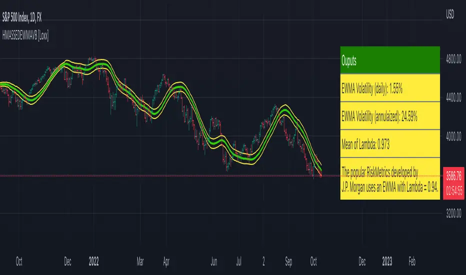
HMA w/ SSE-Dynamic EWMA Volatility Bands [Loxx]This indicator is for educational purposes to lay the groundwork for future closed/open source indicators. Some of thee future indicators will employ parameter estimation methods described below, others will require complex solvers such as the Nelder-Mead algorithm on log likelihood estimations to derive optimal parameter values for omega, gamma, alpha, and beta for GARCH(1,1) MLE and other volatility metrics. For our purposes here, we estimate the rolling lambda (λ) value used to calculate EWMA by minimizing of the sum of the squared errors minus the long-run variance--a rolling window of the one year mean of squared log-returns. In practice, practitioners will use a λ equal to a standardized value put out by institutions such as JP Morgan. Even simpler than this, others use a ratio of (per - 1) / (per + 1) to derive λ where per is the lookback period for EWMA. Due to computation limits in Pine, we'll likely not see a true GARCH(1,1) MLE on Pine for quite some time, but future closed source indicators will contain some very interesting industry hacks to get close by employing modifications to EWMA. Enjoy!
Exponentially weighted volatility and its relationship to GARCH(1,1)
Exponentially weighted volatility--also called exponentially weighted moving average volatility (EWMA)--puts more weight on more recent observations. EWMA is calculated as follows:
σ*2 = λσ(n - 1)^2 + (1 − λ)u(n - 1)^2
The estimate, σn, of the volatility for day n (made at the end of day n − 1) is calculated from σn −1 (the estimate that was made at the end of day n − 2 of the volatility for day n − 1) and u^n−1 (the most recent daily percentage change).
The EWMA approach has the attractive feature that the data storage requirements are modest. At any given time, we need to remember only the current estimate of the variance rate and the most recent observation on the value of the market variable. When we get a new observation on the value of the market variable, we calculate a new daily percentage change to update our estimate of the variance rate. The old estimate of the variance rate and the old value of the market variable can then be discarded.
The EWMA approach is designed to track changes in the volatility. Suppose there is a big move in the market variable on day n − 1 so that u2n−1 is large. This causes our estimate of the current volatility to move upward. The value of λ governs how responsive the estimate of the daily volatility is to the most recent daily percentage change. A low value of λ leads to a great deal of weight being given to the u(n−1)^2 when σn is calculated. In this case, the estimates produced for the volatility on successive days are themselves highly volatile. A high value of λ (i.e., a value close to 1.0) produces estimates of the daily volatility that respond relatively slowly to new information provided by the daily percentage change.
The RiskMetrics database, which was originally created by JPMorgan and made publicly available in 1994, used the EWMA model with λ = 0.94 for updating daily volatility estimates. The company found that, across a range of different market variables, this value of λ gives forecasts of the variance rate that come closest to the realized variance rate. In 2006, RiskMetrics switched to using a long memory model. This is a model where the weights assigned to the u(n -i)^2 as i increases decline less fast than in EWMA.
GARCH(1,1) Model
The EWMA model is a particular case of GARCH(1,1) where γ = 0, α = 1 − λ, and β = λ. The “(1,1)” in GARCH(1,1) indicates that σ^2 is based on the most recent observation of u^2 and the most recent estimate of the variance rate. The more general GARCH(p, q) model calculates σ^2 from the most recent p observations on u2 and the most recent q estimates of the variance rate.7 GARCH(1,1) is by far the most popular of the GARCH models. Setting ω = γVL, the GARCH(1,1) model can also be written:
σ(n)^2 = ω + αu(n-1)^2 + βσ(n-1)^2
What this indicator does
Calculate log returns log(close/close(1))
Calculates Lambda (λ) dynamically by minimizing the sum of squared errors. I've restricted this to the daily timeframe so as to not bloat the code with additional logic required to derive an annualized EWMA historical volatility metric.
After the Lambda is derived, EWMA is calculated one last time and the result is the daily volatility
This daily volatility is multiplied by the source and the multiplier +/- the HMA to create the volatility bands
Finally, daily volatility is multiplied by the square-root of days per year to derive annualized volatility. Years are trading days for the asset, for most everything but crypto, its 252, for crypto is 365.
Garch (1,1) ModelThe Garch (General Autoregressive Conditional Heteroskedasticity) model is a non-linear time series model that uses past data to forecast future variance.
The Garch (1,1) formula is:
Garch = (gamma * Long Run Variance) + (alpha * Squared Lagged Returns) + (beta * Lagged Variance)
The gamma, alpha, and beta values are all weights used in the Garch calculations. According to RiskMetrics by JP Morgan, the optimal beta weight is 0.94, but this figure is highly disputed in the academic realm. The biggest problem academics and economists have with the 0.94 figure is that JP Morgan used monthly data to come to this number, meaning it does not take other time frames into account. Because of the disputed nature of what beta should be, this script will automatically calculate the beta weight for you in real time, taking into account the time frame you're using and realized variance, by using the Minimum Sum of Squared Errors Method.
The gamma and alpha weights are also calculated for you.
Even though the Garch formula provides today's projected variance, today's projected deviation is also calculated. This is done by taking the square root of Garch.
Additionally, if you want to project the variance or deviation for as many days forward as you want, you can.
In order to project the variance and deviation beyond just today, these equations are used:
Projected Variance = Long Run Variance + (alpha + beta)^Days Forward * (Garch - Long Run Variance)
Projected Deviation = sqrt(Projected Variance)
How to use this model:
1st. Decide the type of data you want: Projected Variance in % or Projected Deviation in %.
2nd. Decide how many days you want projected forward. If you input 0, you will get projections for today. If you input 1, you will get projections for tomorrow, and etc.
That's it. If you have any further questions, I left detailed comments in the code explaining each step, as best as I could.