Markov 3D Trend AnalyzerMarkov 3D Trend Analyzer
🔹 What Is a Markov State?
A Markov chain models systems as states with probabilities of transitioning from one state to another. The key property is memorylessness: the next state depends only on the current state, not the full past history. In financial markets, this allows us to study how conditions tend to persist or flip — for example, whether a green candle is more likely to be followed by another green or by a red.
🔹 How This Indicator Uses It
The Markov 3D Trend Analyzer tracks three independent Markov chains:
Direction Chain (short-term): Probability that a green/red candle continues or reverses.
Volatility Chain (mid-term): Probability of volatility staying Low/Medium/High or transitioning between them.
Momentum Chain (structural): Probability of momentum (Bullish, Neutral, Bearish) persisting or flipping.
Each chain is updated dynamically using exponentially weighted probabilities (EMA), which balance the law of large numbers (stability) with adaptivity to new market conditions.
The indicator then classifies each chain’s dominant state and combines them into an actionable summary at the bottom of the table (e.g. “📈 Bullish breakout,” “⚠️ Choppy bearish fakeouts,” “⏳ Trend squeeze / possible reversal”).
🔹 Settings
Direction Lookback / Volatility Lookback / Momentum Lookback
Control the rolling window length (sample size) for each chain. Larger = smoother but slower to adapt.
EMA Weight
Adjusts how much weight is given to recent transitions vs. older history. Lower values adapt faster, higher values stabilize.
Table Position
Choose where the table is displayed on your chart.
Table Size
Adjust the font size for readability.
🔹 How To Consider Using
Contextual tool: Use the summary row to understand the current market condition (trending, mean-reverting, expanding, compressing, continuation, fakeout risk).
Complementary filter: Combine with your existing strategies to confirm or filter signals. For example:
📈 If your breakout strategy fires and the summary says Bullish breakout, that’s confirmation.
⚠️ If it says Choppy fakeouts, be cautious of traps.
Visualization aid: The table lets you see how probabilities shift across direction, volatility, and momentum simultaneously.
⚠️ This indicator is not a signal generator. It is designed to help interpret market states probabilistically. Always use in conjunction with broader analysis and risk management.
🔹 Disclaimer
This script is for educational and informational purposes only. It does not constitute financial advice or a recommendation to buy or sell any security, cryptocurrency, or instrument. Trading involves risk, and past probabilities or behaviors do not guarantee future outcomes. Always conduct your own research and use proper risk management.
Pine Script®指標