MultiType Shifting Predictive Moving Averages (MA) CrossoverJust 2 Moving Averages with adjustable settings and shifting capability, plus signals and predicting continuations.
At the time of publish these different types of MAs are supported:
- SMA (Simple)
- EMA (Exponential)
- DEMA (Double Exponential)
- TEMA (Triple Exponential)
- RMA (Adjusted Exponential)
- WMA (Weighted)
- VWMA (Volume Weighted)
- SWMA (Symmetrically Weighted)
- HMA (Hull)
I'm looking forward to any idea about filtering the signals. Thanks.
Predictive

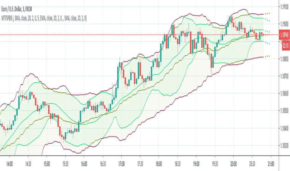
MultiTimeFrame Shifting Predictive Bollinger BandsThis is the optimized version of my MTFSBB indicator with capability of possible bands prediction in case of negative shifting (to the left).
Make me happy by using it and sending me your ideas about the prediction.
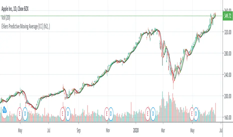
Ehlers Predictive Moving Average [CC]The Predictive Moving Average was created by John Ehlers (Rocket Science For Traders pg 212) and this is one of his first leading indicators. I have been asked by many people for more leading indicators so this one is for you all! Buy when the indicator line is green and sell when it is red.
Let me know if there are other indicators you would like to see me publish or if you want something custom done!
Right Sided Ricker Moving Average And The Gaussian DerivativesIn general gaussian related indicators are built by using the gaussian function in one way or another, for example a gaussian filter is built by using a truncated gaussian function as filter kernel (kernel refer to the set weights) and has many great properties, note that i say truncated because the gaussian function is not supposed to be finite. In general the gaussian function is represented by a symmetrical bell shaped curve, however the gaussian function is parametric, and the user might adjust the position of the peak as well as the width of the curve, an indicator using this parametric approach is the Arnaud Legoux moving average (ALMA) who posses a length parameter controlling the filter length, a peak parameter controlling the position of the peak of the gaussian function as well as a width parameter, those parameters can increase/decrease the lag and smoothness of the moving average output.
However what about the derivatives of the gaussian function ? We don't talk much about them and thats a pity because they are extremely interesting and have many great properties as well, therefore in this post i'll present a low lag moving average based on the modification of the 2nd order derivative of the gaussian function, i believe this post will be extremely informative and i hope you will enjoy reading it, if you are not a math person you can skip the introduction on gaussian derivatives and their properties used as filter kernel.
Gaussian Derivatives And The Ricker Wavelet
The notion of derivative is continuous, so we will stick with the term discrete derivative instead, which just refer to the rate of change in the function, we have a change function in pinescript, and we will be using it to show an approximation of the gaussian function derivatives.
Earlier i used the term 2nd order derivative, here the derivative order refer to the order of differentiation, that is the number of time we apply the change function. For example the 0 (zeroth) order derivative mean no differentiation, the 1st order derivative mean we use differentiation 1 time, that is change(f) , 2nd order mean we use differentiation 2 times, that is change(change(f)) , derivates based on multiple differentiation are called "higher derivative". It will be easier to show a graphic :
Here we can see a normal gaussian function in blue, its scaled 1st order derivative in orange, and its scaled 2nd derivative in green, note that i use scaled because i used multiplication in order for you to see each curve, else it would have been less easy to observe them. The number of time a gaussian function derivative cross 0 is based on the order of differentiation, that is 2nd order = the function crossing 0 two times.
Now we can explain what is the Ricker wavelet, the Ricker wavelet is just the normalized 2nd order derivative of a gaussian function with inverted sign, and unlike the gaussian function the only thing you can change is the width parameter. The formula of the Ricker wavelet is show'n here en.wikipedia.org , where sigma is the width parameter.
The Ricker wavelet has this look :
Because she is shaped like a sombrero the Ricker wavelet is also called "mexican hat wavelet", now what would happen if we used a Ricker wavelet as filter kernel ? The response is that we would end-up with a bandpass filter, in fact the derivatives of the gaussian function would all give the kernel of a bandpass filter, with higher order derivatives making the frequency response of the filter approximate a symmetrical gaussian function, if i recall a filter using the first order derivative of a gaussian function would give a frequency response that is left skewed, this skewness is removed when using higher order derivatives.
The Indicator
I didn't wanted to make a bandpass filter, as lately i'am more interested in low-lag filters, so how can we use the Ricker wavelet to make a low-lag low-pass filter ? The response is by taking the right side of the Ricker wavelet, and since values of the wavelets are negatives near the border we know that the filter passband is non-monotonic, that is we know that the filter will have low-lag as frequencies in the passband will be amplified.
So taking the right side of the Ricker wavelet only mean that t has to be greater than 0 and linearly increasing, thats easy, however the width parameter can be tricky to use, this was already the case with ALMA, so how can we work with it ? First it can be seen that values of width needs to be adjusted based on the filter length.
In red width = 14, in green width = 5. We can see that an higher values of width would give really low weights, when the number of negative weights is too important the filter can have a negative group delay thus becoming predictive, this simply mean that the overshoots/undershoots will be crazy wild and that a great fit will be impossible.
Here two moving averages using the previous described kernels, they don't fit the price well at all ! In order to fix this we can simply define width as a function of the filter length, therefore the parameter "Percentage Width" was introduced, and simply set the width of the Ricker wavelet as p percent of the filter length. Lower values of percent width reduce the lag of the moving average, but lets see precisely how this parameter influence the filter output :
Here the filter length is equal to 100, and the percent width is equal to 60, the fit is quite great, lower values of percent width will increase overshoots, in fact the filter become predictive once the percent width is equal or lower to 50.
Here the percent width is equal to 50. Higher values of percent width reduce the overshoots, and a value of 100 return a filter with no overshoots that is suited to act as a lagging moving average.
Above percent width is set to 100. In order to make use of the predictive side of the filter, it would be great to introduce a forecast option, however this require to find the best forecast horizon period based on length and width, this is no easy task.
Finally lets estimate a least squares moving average with the proposed moving average, you know me...a percent width set to 63 will return a relatively good estimate of the LSMA.
LSMA in green and the proposed moving in red with percent width = 63 and both length = 100.
Conclusion
A new low-lag moving average using a right sided Ricker wavelet as filter kernel has been introduced, we have also seen some properties of gaussian derivatives. You can see that lately i published more moving averages where the user can adjust certain properties of the filter kernel such as curve width for example, if you like those moving averages you can check the Parametric Corrective Linear Moving Averages indicator published last month :
I don't exclude working with pure forms of gaussian derivatives in the future, as i didn't published much oscillators lately.
Thx for reading !

Grand Trend Forecasting - A Simple And Original Approach Today we'll link time series forecasting with signal processing in order to provide an original and funny trend forecasting method, the post share lot of information, if you just want to see how to use the indicator then go to the section "Using The Indicator".
Time series forecasting is an area dealing with the prediction of future values of a series by using a specific model, the model is the main tool that is used for forecasting, and is often an expression based on a set of predictor terms and parameters, for example the linear regression (model) is a 1st order polynomial (expression) using 2 parameters and a predictor variable ax + b . Today we won't be using the linear regression nor the LSMA.
In time series analysis we can describe the time series with a model, in the case of the closing price a simple model could be as follows :
Price = Trend + Cycles + Noise
The variables of the model are the components, such model is additive since we add the component with each others, we should be familiar with each components of the model, the trend represent a simple long term variation of high amplitude, the cycles are periodic fluctuations centered around 0 of varying period and amplitude, the noise component represent shorter term irregular variations with mean 0.
As a trader we are mostly interested by the cycles and the trend, altho the cycles are relatively more technical to trade and can constitute parasitic fluctuations (think about retracements in a trend affecting your trend indicator, causing potential false signals).
If you are curious, in signal processing combining components has a specific name, "synthesis" , here we are dealing with additive synthesis, other type of synthesis are more specific to audio processing and are relatively more complex, but could be used in technical analysis.
So what to do with our components ? If we want to trade the trend, we should estimate right ? Estimating the trend component involve removing the cycle and noise component from the price, if you have read stuff about filters you should know where i'am going, yep, we should use filters, in the case of keeping the trend we can use a simple moving average of relatively high period, and here we go.
However the lag problem, which is recurrent, come back again, we end up with information easier to interpret (here the trend, which is a simple fluctuation such as a line or other smooth curve) at the cost of decision timing, that is unfortunate but as i said the information, here the moving average output, is relatively simple, and could be easily forecasted right ? If you plot a moving average of high period it would be easier for you to forecast its future values. And thats what we aim to do today, provide an estimate of the trend that should be easy to forecast, and should fit to the price relatively well in order to produce forecast that could determine the position of future closing prices observations.
Estimating And Forecasting The Trend
The parameter of the indicator dealing with the estimation of the trend is length , with higher values of length attenuating the cycle and noise component in the price, note however that high values of length can return a really long term trend unlike a simple moving average, so a small value of length, 14 for example can still produce relatively correct estimate of trend.
here length = 14.
The rough estimate of the trend is t in the code, and is an IIR filter, that is, it is based on recursion. Now i'll pass on the filter design explanation but in short, weights are constants, with higher weights allocated to the previous length values of the filter, you can see on the code that the first part of t is similar to an exponential moving average with :
t(n) = 0.9t(n-length) + 0.1*Price
However while the EMA only use the precedent value for the recursion, here we use the precedent length value, this would just output a noisy and really slow output, therefore in order to create a better fit we add : 0.9*(t(n-length) - t(n-2length)) , and this create the rough trend estimate that you can see in blue. On the parameters, 0.9 is used since it gives the best estimate in my opinion, higher values would create more periodic output and lower values would just create a rougher output.
The blue line still contain a residual of the cycle/noise component, this is why it is smoothed with a simple moving average of period length. If you are curious, a filter estimating the trend but still containing noisy fluctuations is called "Notch" filter, such filter would depending on the cutoff remove/attenuate mid term cyclic fluctuations while preserving the trend and the noise, its the opposite of a bandpass filter.
In order to forecast values, we simply sum our trend estimate with the trend estimate change with period equal to the forecasting horizon period, this is a really really simple forecasting method, but it can produce decent results, it can also allows the forecast to start from the last point of the trend estimate.
Using The Indicator
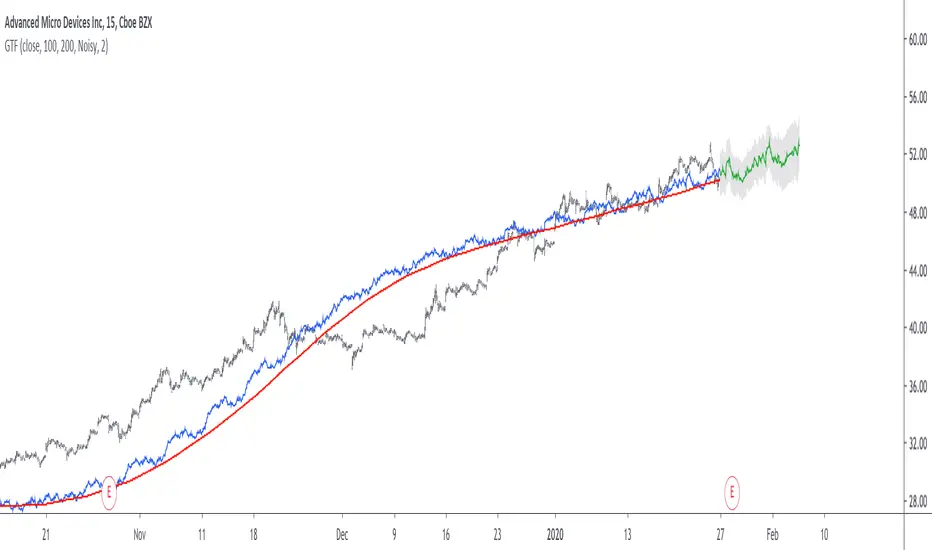
We explained the length parameter in the precedent section, src is the input series which the trend is estimated, forecast determine the forecasting horizon, recommend values for forecast should be equal to length, length/2 or length*2, altho i strongly recommend length.
here length and forecast are both equal to 14 .
The corrective parameter affect the trend estimate, it reduce the overshoot and can led to a curve that might fit better to the price.
The indicator with the non corrective version above, and the corrective one below.
The source parameter determine the source of the forecast, when "Noisy" is selected the source is the blue line, and produce a noisy forecast, when "Smooth" is selected the source is the moving average of t , this create a smoother forecast.
The width interval control...the width of the intervals, they can be seen above and under the forecast plot, they are constructed by adding/subtracting the forecast with the forecast moving average absolute error with respect to the price. Prediction intervals are often associated with a probability (determining the probability of future values being between the interval) here we can't determine such probability with accuracy, this require (i think) an analysis of the forecasting distribution as well as assumptions on the distribution of the forecasting error.
Finally it is possible to see historical forecasts, that is, forecasts previously generated by checking the "Show Historical Forecasts" option.
Examples
Good forecasts mostly occur when the price is close to the trend estimate, this include the following highlighted periods on AMD 15TF with default settings :
We can see the same thing at the end of EURUSD :
However we can't always obtain suitable fits, here it is isn't sufficient on BTCUSD :
We can see wide intervals, we could change length or use the corrective option to get better results, another option is to use a log scale.
We will end the examples with the log SPX, who posses a linear trend, so for example a linear model such as a linear regression would be really adapted, lets see how the indicator perform :
Not a great fit, we could try to use an higher length value and use "Smooth" :
Most recent fits are quite decent.
Conclusions
A forecasting indicator has been presented in this post. The indicator use an original approach toward estimating the trend component in the closing price. Of course i should have given statistics related to the forecasting error, however such analysis is worth doing with better methods and in more advanced environment allowing for optimization.
But we have learned some stuff related to signal processing as well as time series analysis, seeing a time series as the sum of various components is really helpful when it comes to make sense of chaotic and noisy series and is a basic topic in time series analysis.
You can see that in this new year i work harder on the visual of my indicators without trying to fall in the label addict trap, something that i wasn't really doing before, let me know what do you think of it.
Thanks for reading !
Acmillions88 Binary Prediction 1For those who followed me, I have good news for you.
I went into binary options.
The key to binary options is to predict the next candle,
here's a script with high success rate.
Tested on EURUSD 1min.
When the green or red line didn't touch any candle body for a period of time,
then it touches a candle's body.
If the candle is green, a red one is coming soon,
most likely is the next one.
If the candle is red, a green one is coming soon,
most likely is the next one.
Important to note that when the line crosses the body of the candle, it has to be slanted,
meaning the line has to be going up or down.
Please don't ask me why and how it works. Its a secret.
Cheers.

Magick CloudA leading indicator that predicts future price action and shows support and resistance.
Magick Cloud projects 21 bars into the future and uses Fibonacci to predict the targets.
A refreshed version of sKrypt Cloud made by @writner.
Created after testing ~8693 script versions in total and a month of hard work.

Voss Predictive Filter█ OVERVIEW
The Voss Predictive Filter (VPF) is a negative group delay (NGD) filter that anticipates cyclical price movement through phase compensation. The VPF isolates band-limited cyclical components via a bandpass filter, then applies negative group delay to shift the signal's phase forward, causing the output to lead the input by a fraction of the cycle period.
Based on Dr. John F. Ehlers' "Voss Predictive Filter" article in Technical Analysis of Stocks & Commodities (TASC) magazine, the VPF displays a predictive oscillator with optional dynamic threshold bands for identifying significant cycle behavior. The indicator is timeframe-agnostic - the mathematics work identically from tick charts to monthly bars, though shorter timeframes require more careful parameter selection due to noise.
█ CONCEPTS
Bandpass Filtering
A bandpass filter isolates price activity within a specific frequency range, removing both high-frequency noise and low-frequency trend drift. The VPF uses a second-order IIR (Infinite Impulse Response) bandpass filter characterized by the center frequency (the Bandpass Period input) and bandwidth. The center frequency determines which cycle period the filter emphasizes, while bandwidth controls the damping coefficient - how tightly the filter focuses around that frequency. Before filtering, the source is debiased via 2-bar momentum to remove DC offset, ensuring the filter operates around a true zero centerline.
Negative Group Delay Filtering
The predictive capability stems from negative group delay (NGD) - a filter characteristic where output appears to "lead" the input. Most causal filters introduce lag (positive group delay), but by combining the bandpass filter output with appropriately weighted past values, the VPF achieves negative group delay characteristics.
This is a universal NGD filter application for band-limited signals: the bandpass filter isolates the cyclical component of interest, then the NGD stage advances the phase within this limited frequency range to create an anticipatory output. This isn't statistical forecasting; it's phase compensation that shifts the signal's timing forward, causing peaks and troughs to appear before they occur in the bandpass output.
Negative Group Delay Stage
The NGD stage combines the current bandpass output with weighted historical values to produce an output that leads the input. By subtracting a weighted average of past deviations from a scaled version of the current filter value, the algorithm advances the signal's phase: peaks and zero-crossings in the voss output appear before the corresponding events in the bandpass filter.
The prediction order (`3 * Prediction Multiplier`) controls how many past values contribute to the phase advance. Higher orders provide smoother output but reduce the leading effect; lower orders maximize anticipation at the cost of stability.
█ INTERPRETATION
Zero-Line Crossovers
Crossings above zero suggest bullish momentum in the filtered cycle; below zero suggests bearish momentum. Crossings from near-zero regions are most reliable, as extreme excursions need time to return to equilibrium.
Threshold Bands
Threshold bands define "significant" deviation. Breaches indicate unusually strong behavior and can serve as:
• Trend confirmation when aligned with price direction
• Overbought/oversold warnings at extremes
• Trade entry filters (requiring threshold breach in the intended direction)
Threshold Mode affects sensitivity: MAD (outlier-resistant), Standard Deviation (volatility-sensitive), Percentile Rank (fixed probability bands).
Alert Conditions
Four built-in alerts trigger on bar close (no repainting): Above +Threshold (strong bullish cycle), Below -Threshold (strong bearish cycle), Above Zero (bullish phase shift), Below Zero (bearish phase shift).
█ SETTINGS & PARAMETER TUNING
Voss Predictive Filter
• Source : Price series to filter.
• Bandpass Period (1-100): Primary tuning parameter determining which cycle length the filter emphasizes. Short periods (8-15) are more responsive but noisier; medium periods (16-30) balance responsiveness and smoothness; long periods (31-100) focus on longer cycles with more smoothing.
• Bandwidth (0.01-0.45): Controls filter selectivity. Narrow bandwidths (0.01-0.15) isolate specific cycle periods precisely; medium (0.16-0.30) tolerate cycle irregularity; wide (0.31-0.45) capture broader cycle ranges. Shorter periods pair well with narrower bandwidths.
• Prediction Multiplier (2-10): Controls how many past values contribute to the phase advance. Higher values provide smoother output but reduce the leading effect; lower values maximize anticipation at the cost of stability.
Display Settings
Control visibility and colors of the Voss output, bandpass filter, and zero reference lines.
Diagnostics - Dynamic Thresholds
Three methods identify significant signal deviation:
• MAD (Median Absolute Deviation) : Robust, outlier-resistant measure using `k * MAD` where `MAD ≈ 0.6745 * stdev`.
• Standard Deviation : Volatility-sensitive, calculated as `k * stdev` of Voss over the lookback period.
• Percentile Rank : Fixed probability bands using the percentile of |Voss| (e.g., 90% means only 10% of values exceed threshold).
Settings:
• Dynamic Threshold : Toggle threshold bands and set colors.
• Threshold Mode : Select MAD, Standard Deviation, or Percentile Rank.
• Period (2-200): Lookback for threshold calculations. Default 50.
• Multiplier (k) : Scaling for MAD/Standard Deviation modes. Default 1.5.
• Percentile (%) (0-100): For Percentile Rank mode only. Default 90%.
█ LIMITATIONS
Inherent Characteristics
• Residual lag : Despite negative group delay design, some lag remains relative to price action.
• Cyclical markets required : Performs best on instruments with clear cyclical components. Strongly trending markets with little cyclicality produce less useful signals.
• Signal interpretation : Absolute Voss values are instrument-specific. Always interpret relative to adaptive threshold bands, not fixed levels.
Market Conditions to Avoid
• Sudden news events/gaps : Major discontinuities disrupt cycle continuity, causing erratic signals. Requires 1-2 full cycle periods to re-stabilize.
• Low volume/illiquid markets : Sporadic trading produces false cycles from liquidity artifacts. Use only on actively traded instruments during liquid hours.
• Regime changes : During cyclical ↔ trending transitions, watch for persistent extremes without mean reversion, increasing price/indicator divergence, or unresolved threshold breaches.
Parameter Selection Pitfalls
• Mismatched period : If Bandpass Period doesn't match actual market cycles, the filter produces weak signals. Use cycle measurement tools (FFT, autocorrelation, Dominant Cycle) to identify appropriate periods first.
• Overoptimization : Perfect historical fits typically fail forward. Choose robust parameters that work across multiple instruments and timeframes.
█ NOTES
Credits
This indicator is based on concepts from Dr. John F. Ehlers' work on predictive filters and bandpass techniques for technical analysis. Dr. Ehlers has published extensively on applying digital signal processing methods to financial markets in Technical Analysis of Stocks & Commodities (TASC) magazine. His articles on bandpass filters and predictive techniques, particularly the Voss Predictive Filter concept, provided the theoretical foundation for this implementation.
For those interested in the underlying mathematics and DSP concepts:
• Ehlers, J.F. (2001). Rocket Science for Traders: Digital Signal Processing Applications . John Wiley & Sons.
• Various TASC articles by John Ehlers on bandpass filters, cycle analysis, and predictive filtering techniques.
• Ehlers, J.F. "Voss Predictive Filter" - Technical Analysis of Stocks & Commodities magazine.
by ♚@e2e4

Adaptive BB Triple Layer Adaptive BB SD
Band based pullback and pivoting signals ♘♝
Macro Trend sentiment - Outer deviations coloring
Micro trend - Mean Value and normal +/- st.dev colors
Candle Colors - Median Trend
Col Coded Primitive(Basic) Squeeze detection
Sensitive micro break out/down signals derived from basic Mean line crossing (Added some Whipsaw Protection)
Basic Squeeze
Extreme deviations can be turned off for "compact" view
Basic break out/down signals
Indicator needs TESTING
Signal sensitivity and trend recognition need testing/tuning before even considering to use this BB for trading purposes

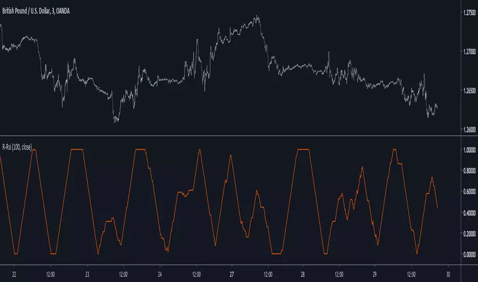
Recursive RsiIntroduction
I have already posted a classic indicator using recursion, it was the stochastic oscillator and recursion helped to get a more predictive and smooth result. Here i will do the same thing with the rsi oscillator but with a different approach. As reminder when using recursion you just use a fraction of the output of a function as input of the same function, i say a fraction because if you feedback the entire output you will just have a periodic function, this is why you average the output with the input.
The Indicator
The indicator will use 50% of the output and 50% of the input, remember that when using feedback always rescale your input, else the effect might be different depending on the market you are in. You can interpret the indicator like a normal rsi except if you plan to use the 80/20 level, depending on length the scale might change, if you need a fixed scale you can always rescale b by using an rsi or stochastic oscillator.
Conclusion
I have presented an rsi oscillator using a different type of recursion structure than the recursive stochastic i posted in the past, the result might be more predictive than the original rsi. Hope you like it and thanks for reading !
Linear Quadratic Convergence Divergence OscillatorIntroduction
I inspired myself from the MACD to present a different oscillator aiming to show more reactive/predictive information. The MACD originally show the relationship between two moving averages by subtracting one of fast period and another one of slow period. In my indicator i will use a similar concept, i will subtract a quadratic least squares moving average with a linear least squares moving average of same period, since the quadratic least squares moving average is faster than the linear one and both methods have low-lag this will result in a reactive oscillator.
LQCD In Details
A quadratic least squares moving average try to fit a quadratic function (parabola) to the price by using the method of least squares, the linear least squares moving average try to fit a line. Non-linear fit tend to minimize the sum of squares in non-linear data, this is why a quadratic method is more reactive. The difference of both filters give us an oscillator, then we apply a simple moving average to this oscillator to provide the signal line, subtracting the oscillator and its signal line give us the histogram, those two last steps are the same used in the MACD.
Length control the period of the quadratic/linear moving average. While the MACD use a signal line for plotting the histogram i also added the option to plot the momentum of the quadratic moving average instead, the result is smoother and reduce irregularities, in order to do so just check the differential option in the parameter box.
The period of the signal line and the momentum are both controlled by the signal parameter.
A predictive approach can be made by subtracting the histogram with the signal line, this process make the histogram way more predictive, in order to do so just check the predictive histogram option in the parameter box.
Predictive histogram with simple histogram option. The differential mode can also be used with the predictive parameter, this result in a smoother but less reactive prediction.
Information Interpretation
The amount of information the MACD can give us is high. We can use the histogram as signal generator, or the if the oscillator is over/under 0, combine the oscillator/signal line with histogram, combinations can provide various systems. Some traders use the histogram as signal generator and use the cross between the histogram and the signal line as a stop signal, this method can avoid some whipsaw trades. The study of divergences with the price is also another method.
Conclusion
This oscillator aim to show the same amount of information as the MACD with a similar calculation method but using different kind of filters as well as eliminating the need to use two separates periods for the moving averages calculation, its still possible to use different periods for the quadratic/linear moving average but the results can be less accurate. This indicator can be used like the MACD.

Dominant Cycle Tuned Rsi BackgroundBackground version of the Dominant Cycle Tuned Rsi Background published here
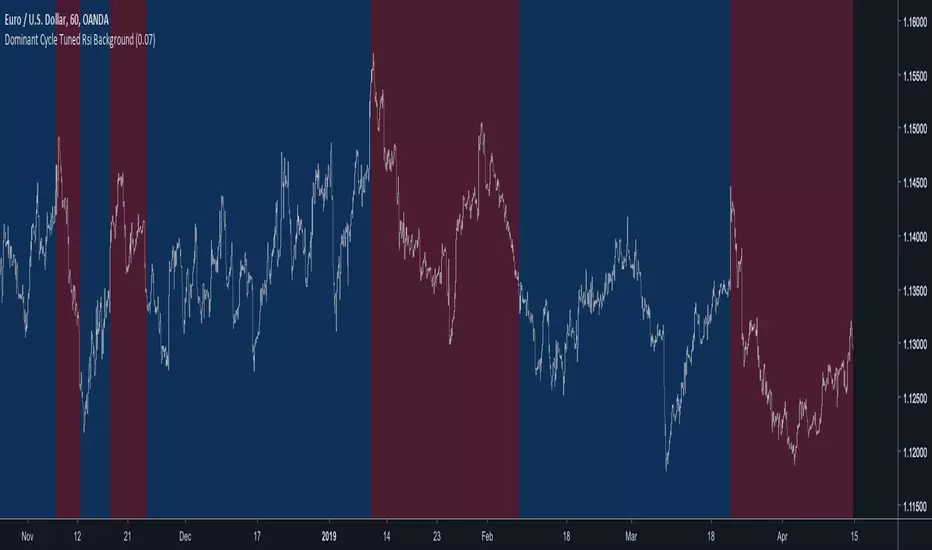
Dominant Cycle Tuned RsiIntroduction
Adaptive technical indicators are importants in a non stationary market, the ability to adapt to a situation can boost the efficiency of your strategy. A lot of methods have been proposed to make technical indicators "smarters" , from the use of variable smoothing constant for exponential smoothing to artificial intelligence.
The dominant cycle tuned rsi depend on the dominant cycle period of the market, such method allow the rsi to return accurate peaks and valleys levels. This indicator is an estimation of the cycle finder tuned rsi proposed by Lars von Thienen published in Decoding the Hidden Market Rhythm/Fine-tuning technical indicators using the dominant market vibration/2010 using the cycle measurement method described by John F.Ehlers in Cybernetic Analysis for Stocks and Futures .
The following section is for information purpose only, it can be technical so you can skip directly to the The Indicator section.
Frequency Estimation and Maximum Entropy Spectral Analysis
“Looks like rain,” said Tom precipitously.
Tom would have been a great weather forecaster, but market patterns are more complex than weather ones. The ability to measure dominant cycles in a complex signal is hard, also a method able to estimate it really fast add even more challenge to the task. First lets talk about the term dominant cycle , signals can be decomposed in a sum of various sine waves of different frequencies and amplitudes, the dominant cycle is considered to be the frequency of the sine wave with the highest amplitude. In general the highest frequencies are those who form the trend (often called fundamentals) , so detrending is used to eliminate those frequencies in order to keep only mid/mid - highs ones.
A lot of methods have been introduced but not that many target market price, Lars von Thienen proposed a method relying on the following processing chain :
Lars von Thienen Method = Input -> Filtering and Detrending -> Discrete Fourier Transform of the result -> Selection using Bartels statistical test -> Output
Thienen said that his method is better than the one proposed by Elhers. The method from Elhers called MESA was originally developed to interpret seismographic information. This method in short involve the estimation of the phase using low amount of information which divided by 360 return the frequency. At first sight there are no relations with the Maximum entropy spectral estimation proposed by Burg J.P. (1967). Maximum Entropy Spectral Analysis. Proceedings of 37th Meeting, Society of Exploration Geophysics, Oklahoma City.
You may also notice that these methods are plotted in the time domain where more classic method such as : power spectrum, spectrogram or FFT are not. The method from Elhers is the one used to tune our rsi.
The Indicator
Our indicator use the dominant cycle frequency to calculate the period of the rsi thus producing an adaptive rsi . When our adaptive rsi cross under 70, price might start a downtrend, else when our adaptive rsi crossover 30, price might start an uptrend. The alpha parameter is a parameter set to be always lower than 1 and greater than 0. Lower values of alpha minimize the number of detected peaks/valleys while higher ones increase the number of those. 0.07 for alpha seems like a great parameter but it can sometimes need to be changed.
The adaptive indicator can also detect small top/bottoms of small periods
Of course the indicator is subject to failures
At the end it is totally dependent of the dominant cycle estimation, which is still a rough method subject to uncertainty.
Conclusion
Tuning your indicator is a great way to make it adapt to the market, but its also a complex way to do so and i'm not that convinced about the complexity/result ratio. The version using chart background will be published separately.
Feel free to tune your indicators with the estimator from elhers and see if it provide a great enhancement :)
Thanks for reading !
References
for the calculation of the dominant cycle estimator originally from www.davenewberg.com
Decoding the Hidden Market Rhythm (2010) Lars von Thienen
Ehlers , J. F. 2004 . Cybernetic Analysis for Stocks and Futures: Cutting-Edge DSP Technology to Improve Your Trading . Wiley

Alpha-Sutte ModelThe Alpha-Sutte model is an ongoing project run by Ansari Saleh Ahmar, a lecturer and researcher at Universitas Negeri Makassar in Indonesia, that attempts to make forecasts for time series like how Arima and Holt-Winters models do. Currently Ahmar and his team have conducted research and published papers comparing the efficacy of the Alpha-Sutte and other models, such as Arima and Holt-Winters, on topics ranging from forecasting Turkey's CPI data, Bitcoin prices, Apple's stock prices, primary energy supply of Indonesia, to infant mortality rates in China.
The Alpha-Sutte model in comparison to the other two models listed above shows promise in providing a more accurate forecast, and the project has been able to receive some of its funding from organizations such as the US Agency for International Development, which is a part of the US Federal Government, so maybe the project has some actual merit.
How it works:
In this model there are four values presented at the top of the window.
1) The first value in blue is the value of the Alpha-Sutte model whose purpose is to forecast the price of the current bar.
2) The second value in yellow is an adaptive version of the Alpha-Sutte model that I made. The purpose of the adaptive Alpha-Sutte model is to expand upon the Alpha-Sutte by allowing new information to be introduced, causing the value to change during the current period, hence the adaptiveness of it.
3) The third value in aqua is the moving average of the low% Sutte line which is a predictive line that is based off of the close and low of the current and previous periods.
4) The fourth value in red is the moving average of the high% Sutte line which is a predictive line that is based off of the close and high of the current and previous periods.
Trend signals:
If low% Sutte (aqua value/line) is greater than high% Sutte (red value/line) then this is a buy signal.
If high% Sutte (red value/line) is greater than low% Sutte (aqua value/line) then this is a sell signal.
Caveat:
Even though this model's purpose is to forecast the future, will it be able to predict periods of large movements? No, of course not, but it will adjust quickly to try to make more accurate forecasts for the next period. This was also a reason why I made an adaptive version of this model to try to reduce some of the discrepancies between the Alpha Sutte and price when there is a large unexpected move.
*WARNING before using this I would highly recommend that you look up "Sutte Indicator" online and read some of the papers about this model before you use this , even though this model has shown merit when compared to Arima and Holt-Winter models this is still an ongoing project.*
Hopefully this project will actually come to something in the near future as the calculation for this time series predictive model is much easier to calculate and program in pine editor than something like an Arima model.
*Also, if you know how to use R language there is a package for the "Alpha-Sutte model".*

acmillions88 Aug2018 predictive indicatorThis is created by accident. The result of one of those "what if I do this".
As you wish...
1) no repaint
2) accurate most of the time
3) predicts the future
I've not tested it live yet but based on its foundation, I know it works!
I have not been creating new scripts for you guys for the past few weeks because
I've been doing tons of research.
Be surprised by what is coming your way. Cheers!

acmillions88 HMCThis script works best on 1 minute timeframe,
while my DHC script works best in 1 hour timeframe.
Look at the chart. Be amazed. I'm amazed too.
Q: Why I created this script?
A: Rahmag found that my DHC V2 works only for higher timeframes, so he
suggested that I modify it for 1 minute timeframe.
Thanks Rahmag.
Cheers!

acmillions88 DHC V2Version 2 of my DHC script.
Sell1 - less probability but higher profit
Buy1 - less probability but higher profit
Sell2 - high probability but lower profit
Buy2 - high probability but lower profit

acmillions88 DHCThis script only works like a charm.
It gives very early signal and it is highly accurate.
Should be the most profitable script I have ever made.

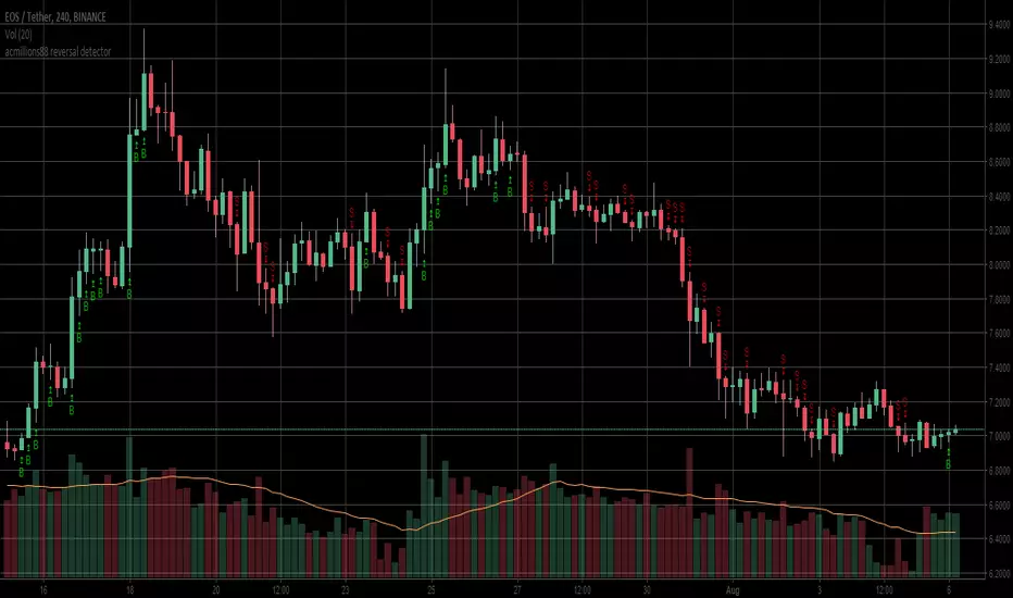
acmillions88 reversal detectorI use a new method to predict trend and made a reversal detector by accident.
Surprisingly, it works very well. More importantly, it is predictive! Hooray!!!
When u see a series of "B" and start seeing an "S", its time to sell.
When u see a series of "S" and start seeing a "B", its time to buy.
Cheers!
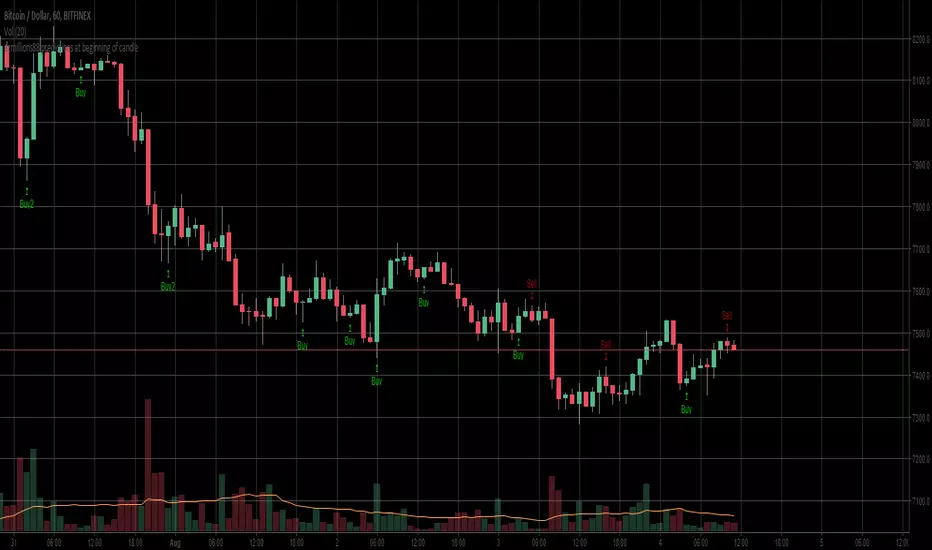
acmillions88 predictions at beginning of new candleJust made a new discovery so I made this script.
It does not depend on trend and it predicts the mini trend at the beginning of the new candle.
The success rate is quite high.
Yes, its another predictive indicator from me. Cheers.
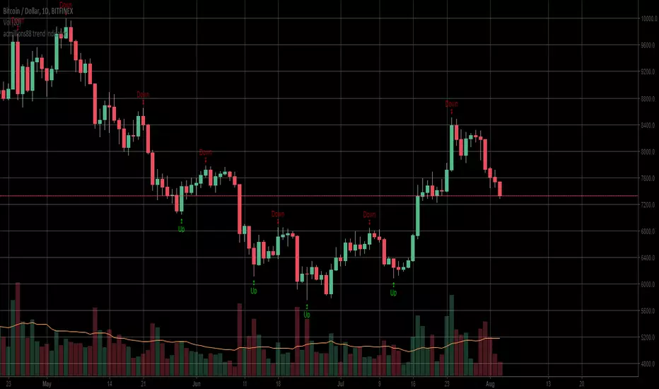
acmillions88 trend indicatorThis should be the best trend indicator I have ever seen. Created by me.
It is not as predictive as my other indicators but its accuracy is extremely high.
acmillions88 crossoverAnother predictive indicator based on crossover.
Green cross predicts mini uptrend.
Red cross predicts mini downtrend.

acmillions88 predictive indicatorsUnlike most scripts, this script actually predicts the mini trends.
