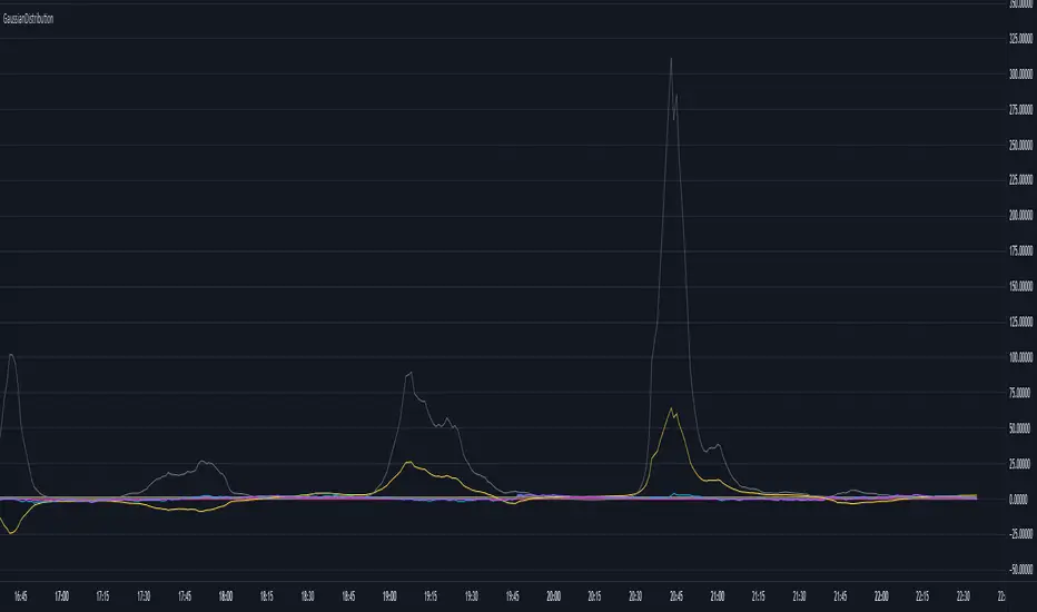
GaussianDistributionLibrary "GaussianDistribution"
This library defines a custom type `distr` representing a Gaussian (or other statistical) distribution.
It provides methods to calculate key statistical moments and scores, including mean, median, mode, standard deviation, variance, skewness, kurtosis, and Z-scores.
This library is useful for analyzing probability distributions in financial data.
Disclaimer:
I am not a mathematician, but I have implemented this library to the best of my understanding and capacity. Please be indulgent as I tried to translate statistical concepts into code as accurately as possible. Feedback, suggestions, and corrections are welcome to improve the reliability and robustness of this library.
mean(source, length)
Calculate the mean (average) of the distribution
Parameters:
source (float) : Distribution source (typically a price or indicator series)
length (int) : Window length for the distribution (must be >= 30 for meaningful statistics)
Returns: Mean (μ)
stdev(source, length)
Calculate the standard deviation (σ) of the distribution
Parameters:
source (float) : Distribution source (typically a price or indicator series)
length (int) : Window length for the distribution (must be >= 30 for meaningful statistics)
Returns: Standard deviation (σ)
skewness(source, length, mean, stdev)
Calculate the skewness (γ₁) of the distribution
Parameters:
source (float) : Distribution source (typically a price or indicator series)
length (int) : Window length for the distribution (must be >= 30 for meaningful statistics)
mean (float) : the mean (average) of the distribution
stdev (float) : the standard deviation (σ) of the distribution
@return Skewness (γ₁)
skewness(source, length)
Overloaded skewness to calculate from source and length
Parameters:
source (float) : Distribution source (typically a price or indicator series)
length (int) : Window length for the distribution (must be >= 30 for meaningful statistics)
@return Skewness (γ₁)
mode(mean, stdev, skewness)
Estimate mode - Most frequent value in the distribution (approximation based on skewness)
Parameters:
mean (float) : the mean (average) of the distribution
stdev (float) : the standard deviation (σ) of the distribution
skewness (float) : the skewness (γ₁) of the distribution
@return Mode
mode(source, length)
Overloaded mode to calculate from source and length
Parameters:
source (float) : Distribution source (typically a price or indicator series)
length (int) : Window length for the distribution (must be >= 30 for meaningful statistics)
@return Mode
median(mean, stdev, skewness)
Estimate median - Middle value of the distribution (approximation)
Parameters:
mean (float) : the mean (average) of the distribution
stdev (float) : the standard deviation (σ) of the distribution
skewness (float) : the skewness (γ₁) of the distribution
@return Median
median(source, length)
Overloaded median to calculate from source and length
Parameters:
source (float) : Distribution source (typically a price or indicator series)
length (int) : Window length for the distribution (must be >= 30 for meaningful statistics)
@return Median
variance(stdev)
Calculate variance (σ²) - Square of the standard deviation
Parameters:
stdev (float) : the standard deviation (σ) of the distribution
@return Variance (σ²)
variance(source, length)
Overloaded variance to calculate from source and length
Parameters:
source (float) : Distribution source (typically a price or indicator series)
length (int) : Window length for the distribution (must be >= 30 for meaningful statistics)
@return Variance (σ²)
kurtosis(source, length, mean, stdev)
Calculate kurtosis (γ₂) - Degree of "tailedness" in the distribution
Parameters:
source (float) : Distribution source (typically a price or indicator series)
length (int) : Window length for the distribution (must be >= 30 for meaningful statistics)
mean (float) : the mean (average) of the distribution
stdev (float) : the standard deviation (σ) of the distribution
@return Kurtosis (γ₂)
kurtosis(source, length)
Overloaded kurtosis to calculate from source and length
Parameters:
source (float) : Distribution source (typically a price or indicator series)
length (int) : Window length for the distribution (must be >= 30 for meaningful statistics)
@return Kurtosis (γ₂)
normal_score(source, mean, stdev)
Calculate Z-score (standard score) assuming a normal distribution
Parameters:
source (float) : Distribution source (typically a price or indicator series)
mean (float) : the mean (average) of the distribution
stdev (float) : the standard deviation (σ) of the distribution
@return Z-Score
normal_score(source, length)
Overloaded normal_score to calculate from source and length
Parameters:
source (float) : Distribution source (typically a price or indicator series)
length (int) : Window length for the distribution (must be >= 30 for meaningful statistics)
@return Z-Score
non_normal_score(source, mean, stdev, skewness, kurtosis)
Calculate adjusted Z-score considering skewness and kurtosis
Parameters:
source (float) : Distribution source (typically a price or indicator series)
mean (float) : the mean (average) of the distribution
stdev (float) : the standard deviation (σ) of the distribution
skewness (float) : the skewness (γ₁) of the distribution
kurtosis (float) : the "tailedness" in the distribution
@return Z-Score
non_normal_score(source, length)
Overloaded non_normal_score to calculate from source and length
Parameters:
source (float) : Distribution source (typically a price or indicator series)
length (int) : Window length for the distribution (must be >= 30 for meaningful statistics)
@return Z-Score
method init(this)
Initialize all statistical fields of the `distr` type
Namespace types: distr
Parameters:
this (distr)
method init(this, source, length)
Overloaded initializer to set source and length
Namespace types: distr
Parameters:
this (distr)
source (float)
length (int)
distr
Custom type to represent a Gaussian distribution
Fields:
source (series float) : Distribution source (typically a price or indicator series)
length (series int) : Window length for the distribution (must be >= 30 for meaningful statistics)
mode (series float) : Most frequent value in the distribution
median (series float) : Middle value separating the greater and lesser halves of the distribution
mean (series float) : μ (1st central moment) - Average of the distribution
stdev (series float) : σ or standard deviation (square root of the variance) - Measure of dispersion
variance (series float) : σ² (2nd central moment) - Squared standard deviation
skewness (series float) : γ₁ (3rd central moment) - Asymmetry of the distribution
kurtosis (series float) : γ₂ (4th central moment) - Degree of "tailedness" relative to a normal distribution
normal_score (series float) : Z-score assuming normal distribution
non_normal_score (series float) : Adjusted Z-score considering skewness and kurtosis
Probability
SimilarityMeasuresLibrary "SimilarityMeasures"
Similarity measures are statistical methods used to quantify the distance between different data sets
or strings. There are various types of similarity measures, including those that compare:
- data points (SSD, Euclidean, Manhattan, Minkowski, Chebyshev, Correlation, Cosine, Camberra, MAE, MSE, Lorentzian, Intersection, Penrose Shape, Meehl),
- strings (Edit(Levenshtein), Lee, Hamming, Jaro),
- probability distributions (Mahalanobis, Fidelity, Bhattacharyya, Hellinger),
- sets (Kumar Hassebrook, Jaccard, Sorensen, Chi Square).
---
These measures are used in various fields such as data analysis, machine learning, and pattern recognition. They
help to compare and analyze similarities and differences between different data sets or strings, which
can be useful for making predictions, classifications, and decisions.
---
References:
en.wikipedia.org
cran.r-project.org
numerics.mathdotnet.com
github.com
github.com
github.com
Encyclopedia of Distances, doi.org
ssd(p, q)
Sum of squared difference for N dimensions.
Parameters:
p (float ) : `array` Vector with first numeric distribution.
q (float ) : `array` Vector with second numeric distribution.
Returns: Measure of distance that calculates the squared euclidean distance.
euclidean(p, q)
Euclidean distance for N dimensions.
Parameters:
p (float ) : `array` Vector with first numeric distribution.
q (float ) : `array` Vector with second numeric distribution.
Returns: Measure of distance that calculates the straight-line (or Euclidean).
manhattan(p, q)
Manhattan distance for N dimensions.
Parameters:
p (float ) : `array` Vector with first numeric distribution.
q (float ) : `array` Vector with second numeric distribution.
Returns: Measure of absolute differences between both points.
minkowski(p, q, p_value)
Minkowsky Distance for N dimensions.
Parameters:
p (float ) : `array` Vector with first numeric distribution.
q (float ) : `array` Vector with second numeric distribution.
p_value (float) : `float` P value, default=1.0(1: manhatan, 2: euclidean), does not support chebychev.
Returns: Measure of similarity in the normed vector space.
chebyshev(p, q)
Chebyshev distance for N dimensions.
Parameters:
p (float ) : `array` Vector with first numeric distribution.
q (float ) : `array` Vector with second numeric distribution.
Returns: Measure of maximum absolute difference.
correlation(p, q)
Correlation distance for N dimensions.
Parameters:
p (float ) : `array` Vector with first numeric distribution.
q (float ) : `array` Vector with second numeric distribution.
Returns: Measure of maximum absolute difference.
cosine(p, q)
Cosine distance between provided vectors.
Parameters:
p (float ) : `array` 1D Vector.
q (float ) : `array` 1D Vector.
Returns: The Cosine distance between vectors `p` and `q`.
---
angiogenesis.dkfz.de
camberra(p, q)
Camberra distance for N dimensions.
Parameters:
p (float ) : `array` Vector with first numeric distribution.
q (float ) : `array` Vector with second numeric distribution.
Returns: Weighted measure of absolute differences between both points.
mae(p, q)
Mean absolute error is a normalized version of the sum of absolute difference (manhattan).
Parameters:
p (float ) : `array` Vector with first numeric distribution.
q (float ) : `array` Vector with second numeric distribution.
Returns: Mean absolute error of vectors `p` and `q`.
mse(p, q)
Mean squared error is a normalized version of the sum of squared difference.
Parameters:
p (float ) : `array` Vector with first numeric distribution.
q (float ) : `array` Vector with second numeric distribution.
Returns: Mean squared error of vectors `p` and `q`.
lorentzian(p, q)
Lorentzian distance between provided vectors.
Parameters:
p (float ) : `array` Vector with first numeric distribution.
q (float ) : `array` Vector with second numeric distribution.
Returns: Lorentzian distance of vectors `p` and `q`.
---
angiogenesis.dkfz.de
intersection(p, q)
Intersection distance between provided vectors.
Parameters:
p (float ) : `array` Vector with first numeric distribution.
q (float ) : `array` Vector with second numeric distribution.
Returns: Intersection distance of vectors `p` and `q`.
---
angiogenesis.dkfz.de
penrose(p, q)
Penrose Shape distance between provided vectors.
Parameters:
p (float ) : `array` Vector with first numeric distribution.
q (float ) : `array` Vector with second numeric distribution.
Returns: Penrose shape distance of vectors `p` and `q`.
---
angiogenesis.dkfz.de
meehl(p, q)
Meehl distance between provided vectors.
Parameters:
p (float ) : `array` Vector with first numeric distribution.
q (float ) : `array` Vector with second numeric distribution.
Returns: Meehl distance of vectors `p` and `q`.
---
angiogenesis.dkfz.de
edit(x, y)
Edit (aka Levenshtein) distance for indexed strings.
Parameters:
x (int ) : `array` Indexed array.
y (int ) : `array` Indexed array.
Returns: Number of deletions, insertions, or substitutions required to transform source string into target string.
---
generated description:
The Edit distance is a measure of similarity used to compare two strings. It is defined as the minimum number of
operations (insertions, deletions, or substitutions) required to transform one string into another. The operations
are performed on the characters of the strings, and the cost of each operation depends on the specific algorithm
used.
The Edit distance is widely used in various applications such as spell checking, text similarity, and machine
translation. It can also be used for other purposes like finding the closest match between two strings or
identifying the common prefixes or suffixes between them.
---
github.com
www.red-gate.com
planetcalc.com
lee(x, y, dsize)
Distance between two indexed strings of equal length.
Parameters:
x (int ) : `array` Indexed array.
y (int ) : `array` Indexed array.
dsize (int) : `int` Dictionary size.
Returns: Distance between two strings by accounting for dictionary size.
---
www.johndcook.com
hamming(x, y)
Distance between two indexed strings of equal length.
Parameters:
x (int ) : `array` Indexed array.
y (int ) : `array` Indexed array.
Returns: Length of different components on both sequences.
---
en.wikipedia.org
jaro(x, y)
Distance between two indexed strings.
Parameters:
x (int ) : `array` Indexed array.
y (int ) : `array` Indexed array.
Returns: Measure of two strings' similarity: the higher the value, the more similar the strings are.
The score is normalized such that `0` equates to no similarities and `1` is an exact match.
---
rosettacode.org
mahalanobis(p, q, VI)
Mahalanobis distance between two vectors with population inverse covariance matrix.
Parameters:
p (float ) : `array` 1D Vector.
q (float ) : `array` 1D Vector.
VI (matrix) : `matrix` Inverse of the covariance matrix.
Returns: The mahalanobis distance between vectors `p` and `q`.
---
people.revoledu.com
stat.ethz.ch
docs.scipy.org
fidelity(p, q)
Fidelity distance between provided vectors.
Parameters:
p (float ) : `array` 1D Vector.
q (float ) : `array` 1D Vector.
Returns: The Bhattacharyya Coefficient between vectors `p` and `q`.
---
en.wikipedia.org
bhattacharyya(p, q)
Bhattacharyya distance between provided vectors.
Parameters:
p (float ) : `array` 1D Vector.
q (float ) : `array` 1D Vector.
Returns: The Bhattacharyya distance between vectors `p` and `q`.
---
en.wikipedia.org
hellinger(p, q)
Hellinger distance between provided vectors.
Parameters:
p (float ) : `array` 1D Vector.
q (float ) : `array` 1D Vector.
Returns: The hellinger distance between vectors `p` and `q`.
---
en.wikipedia.org
jamesmccaffrey.wordpress.com
kumar_hassebrook(p, q)
Kumar Hassebrook distance between provided vectors.
Parameters:
p (float ) : `array` 1D Vector.
q (float ) : `array` 1D Vector.
Returns: The Kumar Hassebrook distance between vectors `p` and `q`.
---
github.com
jaccard(p, q)
Jaccard distance between provided vectors.
Parameters:
p (float ) : `array` 1D Vector.
q (float ) : `array` 1D Vector.
Returns: The Jaccard distance between vectors `p` and `q`.
---
github.com
sorensen(p, q)
Sorensen distance between provided vectors.
Parameters:
p (float ) : `array` 1D Vector.
q (float ) : `array` 1D Vector.
Returns: The Sorensen distance between vectors `p` and `q`.
---
people.revoledu.com
chi_square(p, q, eps)
Chi Square distance between provided vectors.
Parameters:
p (float ) : `array` 1D Vector.
q (float ) : `array` 1D Vector.
eps (float)
Returns: The Chi Square distance between vectors `p` and `q`.
---
uw.pressbooks.pub
stats.stackexchange.com
www.itl.nist.gov
kulczynsky(p, q, eps)
Kulczynsky distance between provided vectors.
Parameters:
p (float ) : `array` 1D Vector.
q (float ) : `array` 1D Vector.
eps (float)
Returns: The Kulczynsky distance between vectors `p` and `q`.
---
github.com

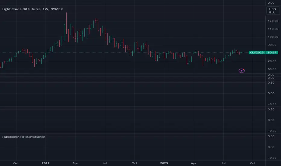
FunctionMatrixCovarianceLibrary "FunctionMatrixCovariance"
In probability theory and statistics, a covariance matrix (also known as auto-covariance matrix, dispersion matrix, variance matrix, or variance–covariance matrix) is a square matrix giving the covariance between each pair of elements of a given random vector.
Intuitively, the covariance matrix generalizes the notion of variance to multiple dimensions. As an example, the variation in a collection of random points in two-dimensional space cannot be characterized fully by a single number, nor would the variances in the `x` and `y` directions contain all of the necessary information; a `2 × 2` matrix would be necessary to fully characterize the two-dimensional variation.
Any covariance matrix is symmetric and positive semi-definite and its main diagonal contains variances (i.e., the covariance of each element with itself).
The covariance matrix of a random vector `X` is typically denoted by `Kxx`, `Σ` or `S`.
~wikipedia.
method cov(M, bias)
Estimate Covariance matrix with provided data.
Namespace types: matrix
Parameters:
M (matrix) : `matrix` Matrix with vectors in column order.
bias (bool)
Returns: Covariance matrix of provided vectors.
---
en.wikipedia.org
numpy.org
BenfordsLawLibrary "BenfordsLaw"
Methods to deal with Benford's law which states that a distribution of first and higher order digits
of numerical strings has a characteristic pattern.
"Benford's law is an observation about the leading digits of the numbers found in real-world data sets.
Intuitively, one might expect that the leading digits of these numbers would be uniformly distributed so that
each of the digits from 1 to 9 is equally likely to appear. In fact, it is often the case that 1 occurs more
frequently than 2, 2 more frequently than 3, and so on. This observation is a simplified version of Benford's law.
More precisely, the law gives a prediction of the frequency of leading digits using base-10 logarithms that
predicts specific frequencies which decrease as the digits increase from 1 to 9." ~(2)
---
reference:
- 1: en.wikipedia.org
- 2: brilliant.org
- 4: github.com
cumsum_difference(a, b)
Calculate the cumulative sum difference of two arrays of same size.
Parameters:
a (float ) : `array` List of values.
b (float ) : `array` List of values.
Returns: List with CumSum Difference between arrays.
fractional_int(number)
Transform a floating number including its fractional part to integer form ex:. `1.2345 -> 12345`.
Parameters:
number (float) : `float` The number to transform.
Returns: Transformed number.
split_to_digits(number, reverse)
Transforms a integer number into a list of its digits.
Parameters:
number (int) : `int` Number to transform.
reverse (bool) : `bool` `default=true`, Reverse the order of the digits, if true, last will be first.
Returns: Transformed number digits list.
digit_in(number, digit)
Digit at index.
Parameters:
number (int) : `int` Number to parse.
digit (int) : `int` `default=0`, Index of digit.
Returns: Digit found at the index.
digits_from(data, dindex)
Process a list of `int` values and get the list of digits.
Parameters:
data (int ) : `array` List of numbers.
dindex (int) : `int` `default=0`, Index of digit.
Returns: List of digits at the index.
digit_counters(digits)
Score digits.
Parameters:
digits (int ) : `array` List of digits.
Returns: List of counters per digit (1-9).
digit_distribution(counters)
Calculates the frequency distribution based on counters provided.
Parameters:
counters (int ) : `array` List of counters, must have size(9).
Returns: Distribution of the frequency of the digits.
digit_p(digit)
Expected probability for digit according to Benford.
Parameters:
digit (int) : `int` Digit number reference in range `1 -> 9`.
Returns: Probability of digit according to Benford's law.
benfords_distribution()
Calculated Expected distribution per digit according to Benford's Law.
Returns: List with the expected distribution.
benfords_distribution_aprox()
Aproximate Expected distribution per digit according to Benford's Law.
Returns: List with the expected distribution.
test_benfords(digits, calculate_benfords)
Tests Benford's Law on provided list of digits.
Parameters:
digits (int ) : `array` List of digits.
calculate_benfords (bool)
Returns: Tuple with:
- Counters: Score of each digit.
- Sample distribution: Frequency for each digit.
- Expected distribution: Expected frequency according to Benford's.
- Cumulative Sum of difference:
to_table(digits, _text_color, _border_color, _frame_color)
Parameters:
digits (int )
_text_color (color)
_border_color (color)
_frame_color (color)

MarkovChainLibrary "MarkovChain"
Generic Markov Chain type functions.
---
A Markov chain or Markov process is a stochastic model describing a sequence of possible events in which the
probability of each event depends only on the state attained in the previous event.
---
reference:
Understanding Markov Chains, Examples and Applications. Second Edition. Book by Nicolas Privault.
en.wikipedia.org
www.geeksforgeeks.org
towardsdatascience.com
github.com
stats.stackexchange.com
timeseriesreasoning.com
www.ris-ai.com
github.com
gist.github.com
github.com
gist.github.com
writings.stephenwolfram.com
kevingal.com
towardsdatascience.com
spedygiorgio.github.io
github.com
www.projectrhea.org
method to_string(this)
Translate a Markov Chain object to a string format.
Namespace types: MC
Parameters:
this (MC) : `MC` . Markov Chain object.
Returns: string
method to_table(this, position, text_color, text_size)
Namespace types: MC
Parameters:
this (MC)
position (string)
text_color (color)
text_size (string)
method create_transition_matrix(this)
Namespace types: MC
Parameters:
this (MC)
method generate_transition_matrix(this)
Namespace types: MC
Parameters:
this (MC)
new_chain(states, name)
Parameters:
states (state )
name (string)
from_data(data, name)
Parameters:
data (string )
name (string)
method probability_at_step(this, target_step)
Namespace types: MC
Parameters:
this (MC)
target_step (int)
method state_at_step(this, start_state, target_state, target_step)
Namespace types: MC
Parameters:
this (MC)
start_state (int)
target_state (int)
target_step (int)
method forward(this, obs)
Namespace types: HMC
Parameters:
this (HMC)
obs (int )
method backward(this, obs)
Namespace types: HMC
Parameters:
this (HMC)
obs (int )
method viterbi(this, observations)
Namespace types: HMC
Parameters:
this (HMC)
observations (int )
method baumwelch(this, observations)
Namespace types: HMC
Parameters:
this (HMC)
observations (int )
Node
Target node.
Fields:
index (series int) : . Key index of the node.
probability (series float) : . Probability rate of activation.
state
State reference.
Fields:
name (series string) : . Name of the state.
index (series int) : . Key index of the state.
target_nodes (Node ) : . List of index references and probabilities to target states.
MC
Markov Chain reference object.
Fields:
name (series string) : . Name of the chain.
states (state ) : . List of state nodes and its name, index, targets and transition probabilities.
size (series int) : . Number of unique states
transitions (matrix) : . Transition matrix
HMC
Hidden Markov Chain reference object.
Fields:
name (series string) : . Name of thehidden chain.
states_hidden (state ) : . List of state nodes and its name, index, targets and transition probabilities.
states_obs (state ) : . List of state nodes and its name, index, targets and transition probabilities.
transitions (matrix) : . Transition matrix
emissions (matrix) : . Emission matrix
initial_distribution (float )

FunctionProbabilityViterbiLibrary "FunctionProbabilityViterbi"
The Viterbi Algorithm calculates the most likely sequence of hidden states *(called Viterbi path)*
that results in a sequence of observed events.
viterbi(observations, transitions, emissions, initial_distribution)
Calculate most probable path in a Markov model.
Parameters:
observations (int ) : array . Observation states data.
transitions (matrix) : matrix . Transition probability table, (HxH, H:Hidden states).
emissions (matrix) : matrix . Emission probability table, (OxH, O:Observed states).
initial_distribution (float ) : array . Initial probability distribution for the hidden states.
Returns: array. Most probable path.

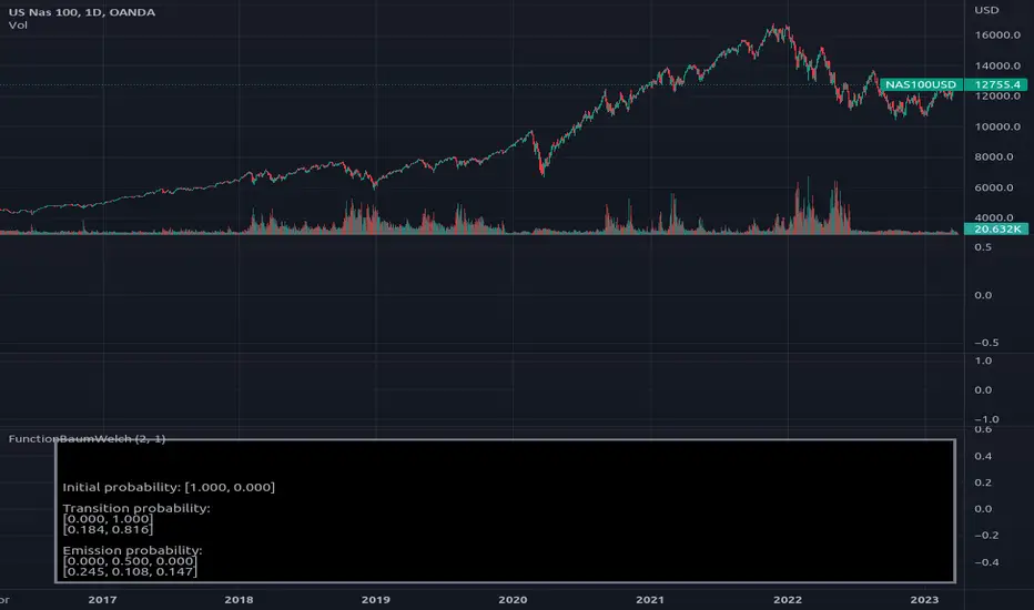
FunctionBaumWelchLibrary "FunctionBaumWelch"
Baum-Welch Algorithm, also known as Forward-Backward Algorithm, uses the well known EM algorithm
to find the maximum likelihood estimate of the parameters of a hidden Markov model given a set of observed
feature vectors.
---
### Function List:
> `forward (array pi, matrix a, matrix b, array obs)`
> `forward (array pi, matrix a, matrix b, array obs, bool scaling)`
> `backward (matrix a, matrix b, array obs)`
> `backward (matrix a, matrix b, array obs, array c)`
> `baumwelch (array observations, int nstates)`
> `baumwelch (array observations, array pi, matrix a, matrix b)`
---
### Reference:
> en.wikipedia.org
> github.com
> en.wikipedia.org
> www.rdocumentation.org
> www.rdocumentation.org
forward(pi, a, b, obs)
Computes forward probabilities for state `X` up to observation at time `k`, is defined as the
probability of observing sequence of observations `e_1 ... e_k` and that the state at time `k` is `X`.
Parameters:
pi (float ) : Initial probabilities.
a (matrix) : Transmissions, hidden transition matrix a or alpha = transition probability matrix of changing
states given a state matrix is size (M x M) where M is number of states.
b (matrix) : Emissions, matrix of observation probabilities b or beta = observation probabilities. Given
state matrix is size (M x O) where M is number of states and O is number of different
possible observations.
obs (int ) : List with actual state observation data.
Returns: - `matrix _alpha`: Forward probabilities. The probabilities are given on a logarithmic scale (natural logarithm). The first
dimension refers to the state and the second dimension to time.
forward(pi, a, b, obs, scaling)
Computes forward probabilities for state `X` up to observation at time `k`, is defined as the
probability of observing sequence of observations `e_1 ... e_k` and that the state at time `k` is `X`.
Parameters:
pi (float ) : Initial probabilities.
a (matrix) : Transmissions, hidden transition matrix a or alpha = transition probability matrix of changing
states given a state matrix is size (M x M) where M is number of states.
b (matrix) : Emissions, matrix of observation probabilities b or beta = observation probabilities. Given
state matrix is size (M x O) where M is number of states and O is number of different
possible observations.
obs (int ) : List with actual state observation data.
scaling (bool) : Normalize `alpha` scale.
Returns: - #### Tuple with:
> - `matrix _alpha`: Forward probabilities. The probabilities are given on a logarithmic scale (natural logarithm). The first
dimension refers to the state and the second dimension to time.
> - `array _c`: Array with normalization scale.
backward(a, b, obs)
Computes backward probabilities for state `X` and observation at time `k`, is defined as the probability of observing the sequence of observations `e_k+1, ... , e_n` under the condition that the state at time `k` is `X`.
Parameters:
a (matrix) : Transmissions, hidden transition matrix a or alpha = transition probability matrix of changing states
given a state matrix is size (M x M) where M is number of states
b (matrix) : Emissions, matrix of observation probabilities b or beta = observation probabilities. given state
matrix is size (M x O) where M is number of states and O is number of different possible observations
obs (int ) : Array with actual state observation data.
Returns: - `matrix _beta`: Backward probabilities. The probabilities are given on a logarithmic scale (natural logarithm). The first dimension refers to the state and the second dimension to time.
backward(a, b, obs, c)
Computes backward probabilities for state `X` and observation at time `k`, is defined as the probability of observing the sequence of observations `e_k+1, ... , e_n` under the condition that the state at time `k` is `X`.
Parameters:
a (matrix) : Transmissions, hidden transition matrix a or alpha = transition probability matrix of changing states
given a state matrix is size (M x M) where M is number of states
b (matrix) : Emissions, matrix of observation probabilities b or beta = observation probabilities. given state
matrix is size (M x O) where M is number of states and O is number of different possible observations
obs (int ) : Array with actual state observation data.
c (float ) : Array with Normalization scaling coefficients.
Returns: - `matrix _beta`: Backward probabilities. The probabilities are given on a logarithmic scale (natural logarithm). The first dimension refers to the state and the second dimension to time.
baumwelch(observations, nstates)
**(Random Initialization)** Baum–Welch algorithm is a special case of the expectation–maximization algorithm used to find the
unknown parameters of a hidden Markov model (HMM). It makes use of the forward-backward algorithm
to compute the statistics for the expectation step.
Parameters:
observations (int ) : List of observed states.
nstates (int)
Returns: - #### Tuple with:
> - `array _pi`: Initial probability distribution.
> - `matrix _a`: Transition probability matrix.
> - `matrix _b`: Emission probability matrix.
---
requires: `import RicardoSantos/WIPTensor/2 as Tensor`
baumwelch(observations, pi, a, b)
Baum–Welch algorithm is a special case of the expectation–maximization algorithm used to find the
unknown parameters of a hidden Markov model (HMM). It makes use of the forward-backward algorithm
to compute the statistics for the expectation step.
Parameters:
observations (int ) : List of observed states.
pi (float ) : Initial probaility distribution.
a (matrix) : Transmissions, hidden transition matrix a or alpha = transition probability matrix of changing states
given a state matrix is size (M x M) where M is number of states
b (matrix) : Emissions, matrix of observation probabilities b or beta = observation probabilities. given state
matrix is size (M x O) where M is number of states and O is number of different possible observations
Returns: - #### Tuple with:
> - `array _pi`: Initial probability distribution.
> - `matrix _a`: Transition probability matrix.
> - `matrix _b`: Emission probability matrix.
---
requires: `import RicardoSantos/WIPTensor/2 as Tensor`
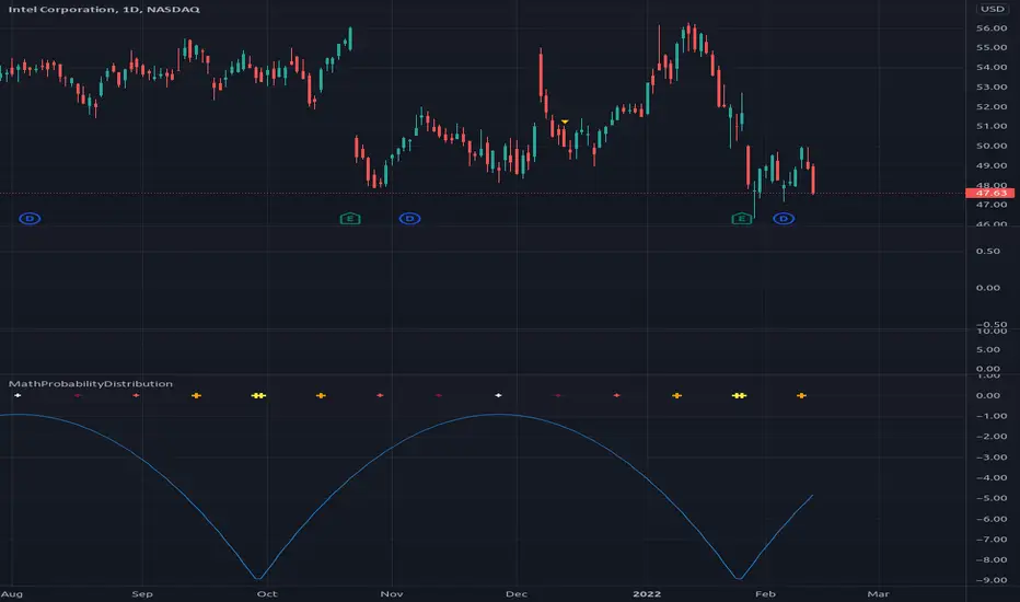
MathProbabilityDistributionLibrary "MathProbabilityDistribution"
Probability Distribution Functions.
name(idx) Indexed names helper function.
Parameters:
idx : int, position in the range (0, 6).
Returns: string, distribution name.
usage:
.name(1)
Notes:
(0) => 'StdNormal'
(1) => 'Normal'
(2) => 'Skew Normal'
(3) => 'Student T'
(4) => 'Skew Student T'
(5) => 'GED'
(6) => 'Skew GED'
zscore(position, mean, deviation) Z-score helper function for x calculation.
Parameters:
position : float, position.
mean : float, mean.
deviation : float, standard deviation.
Returns: float, z-score.
usage:
.zscore(1.5, 2.0, 1.0)
std_normal(position) Standard Normal Distribution.
Parameters:
position : float, position.
Returns: float, probability density.
usage:
.std_normal(0.6)
normal(position, mean, scale) Normal Distribution.
Parameters:
position : float, position in the distribution.
mean : float, mean of the distribution, default=0.0 for standard distribution.
scale : float, scale of the distribution, default=1.0 for standard distribution.
Returns: float, probability density.
usage:
.normal(0.6)
skew_normal(position, skew, mean, scale) Skew Normal Distribution.
Parameters:
position : float, position in the distribution.
skew : float, skewness of the distribution.
mean : float, mean of the distribution, default=0.0 for standard distribution.
scale : float, scale of the distribution, default=1.0 for standard distribution.
Returns: float, probability density.
usage:
.skew_normal(0.8, -2.0)
ged(position, shape, mean, scale) Generalized Error Distribution.
Parameters:
position : float, position.
shape : float, shape.
mean : float, mean, default=0.0 for standard distribution.
scale : float, scale, default=1.0 for standard distribution.
Returns: float, probability.
usage:
.ged(0.8, -2.0)
skew_ged(position, shape, skew, mean, scale) Skew Generalized Error Distribution.
Parameters:
position : float, position.
shape : float, shape.
skew : float, skew.
mean : float, mean, default=0.0 for standard distribution.
scale : float, scale, default=1.0 for standard distribution.
Returns: float, probability.
usage:
.skew_ged(0.8, 2.0, 1.0)
student_t(position, shape, mean, scale) Student-T Distribution.
Parameters:
position : float, position.
shape : float, shape.
mean : float, mean, default=0.0 for standard distribution.
scale : float, scale, default=1.0 for standard distribution.
Returns: float, probability.
usage:
.student_t(0.8, 2.0, 1.0)
skew_student_t(position, shape, skew, mean, scale) Skew Student-T Distribution.
Parameters:
position : float, position.
shape : float, shape.
skew : float, skew.
mean : float, mean, default=0.0 for standard distribution.
scale : float, scale, default=1.0 for standard distribution.
Returns: float, probability.
usage:
.skew_student_t(0.8, 2.0, 1.0)
select(distribution, position, mean, scale, shape, skew, log) Conditional Distribution.
Parameters:
distribution : string, distribution name.
position : float, position.
mean : float, mean, default=0.0 for standard distribution.
scale : float, scale, default=1.0 for standard distribution.
shape : float, shape.
skew : float, skew.
log : bool, if true apply log() to the result.
Returns: float, probability.
usage:
.select('StdNormal', __CYCLE4F__, log=true)
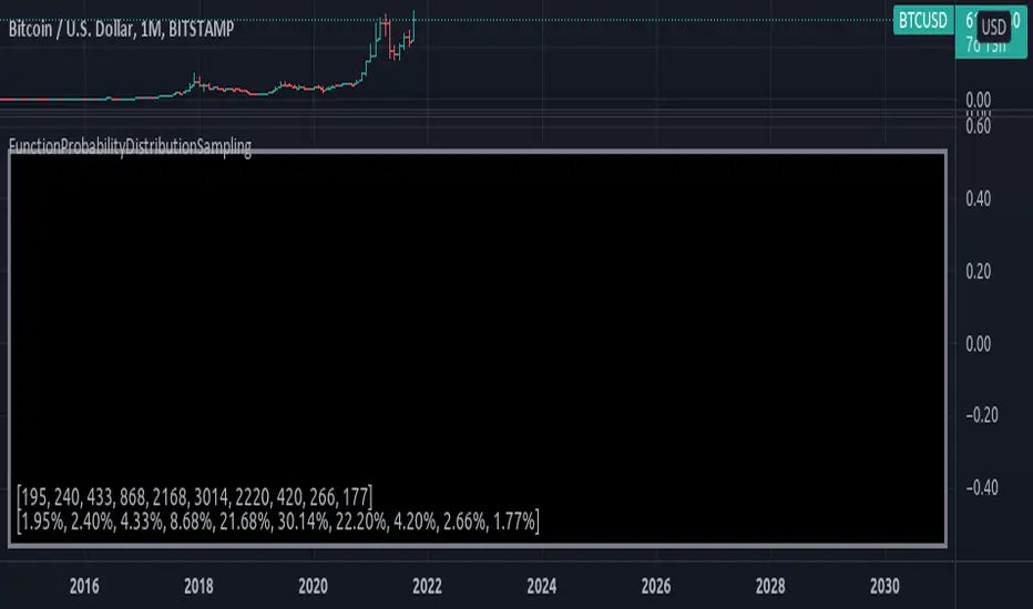
FunctionProbabilityDistributionSamplingLibrary "FunctionProbabilityDistributionSampling"
Methods for probability distribution sampling selection.
sample(probabilities) Computes a random selected index from a probability distribution.
Parameters:
probabilities : float array, probabilities of sample.
Returns: int.
FunctionSMCMCLibrary "FunctionSMCMC"
Methods to implement Markov Chain Monte Carlo Simulation (MCMC)
markov_chain(weights, actions, target_path, position, last_value) a basic implementation of the markov chain algorithm
Parameters:
weights : float array, weights of the Markov Chain.
actions : float array, actions of the Markov Chain.
target_path : float array, target path array.
position : int, index of the path.
last_value : float, base value to increment.
Returns: void, updates target array
mcmc(weights, actions, start_value, n_iterations) uses a monte carlo algorithm to simulate a markov chain at each step.
Parameters:
weights : float array, weights of the Markov Chain.
actions : float array, actions of the Markov Chain.
start_value : float, base value to start simulation.
n_iterations : integer, number of iterations to run.
Returns: float array with path.

ProbabilityLibrary "Probability"
erf(value) Complementary error function
Parameters:
value : float, value to test.
Returns: float
ierf_mcgiles(value) Computes the inverse error function using the Mc Giles method, sacrifices accuracy for speed.
Parameters:
value : float, -1.0 >= _value >= 1.0 range, value to test.
Returns: float
ierf_double(value) computes the inverse error function using the Newton method with double refinement.
Parameters:
value : float, -1. > _value > 1. range, _value to test.
Returns: float
ierf(value) computes the inverse error function using the Newton method.
Parameters:
value : float, -1. > _value > 1. range, _value to test.
Returns: float
complement(probability) probability that the event will not occur.
Parameters:
probability : float, 0 >=_p >= 1, probability of event.
Returns: float
entropy_gini_impurity_single(probability) Gini Inbalance or Gini index for a given probability.
Parameters:
probability : float, 0>=x>=1, probability of event.
Returns: float
entropy_gini_impurity(events) Gini Inbalance or Gini index for a series of events.
Parameters:
events : float , 0>=x>=1, array with event probability's.
Returns: float
entropy_shannon_single(probability) Entropy information value of the probability of a single event.
Parameters:
probability : float, 0>=x>=1, probability value.
Returns: float, value as bits of information.
entropy_shannon(events) Entropy information value of a distribution of events.
Parameters:
events : float , 0>=x>=1, array with probability's.
Returns: float
inequality_chebyshev(n_stdeviations) Calculates Chebyshev Inequality.
Parameters:
n_stdeviations : float, positive over or equal to 1.0
Returns: float
inequality_chebyshev_distribution(mean, std) Calculates Chebyshev Inequality.
Parameters:
mean : float, mean of a distribution
std : float, standard deviation of a distribution
Returns: float
inequality_chebyshev_sample(data_sample) Calculates Chebyshev Inequality for a array of values.
Parameters:
data_sample : float , array of numbers.
Returns: float
intersection_of_independent_events(events) Probability that all arguments will happen when neither outcome
is affected by the other (accepts 1 or more arguments)
Parameters:
events : float , 0 >= _p >= 1, list of event probabilities.
Returns: float
union_of_independent_events(events) Probability that either one of the arguments will happen when neither outcome
is affected by the other (accepts 1 or more arguments)
Parameters:
events : float , 0 >= _p >= 1, list of event probabilities.
Returns: float
mass_function(sample, n_bins) Probabilities for each bin in the range of sample.
Parameters:
sample : float , samples to pool probabilities.
n_bins : int, number of bins to split the range
@return float
cumulative_distribution_function(mean, stdev, value) Use the CDF to determine the probability that a random observation
that is taken from the population will be less than or equal to a certain value.
Or returns the area of probability for a known value in a normal distribution.
Parameters:
mean : float, samples to pool probabilities.
stdev : float, number of bins to split the range
value : float, limit at which to stop.
Returns: float
transition_matrix(distribution) Transition matrix for the suplied distribution.
Parameters:
distribution : float , array with probability distribution. ex:.
Returns: float
diffusion_matrix(transition_matrix, dimension, target_step) Probability of reaching target_state at target_step after starting from start_state
Parameters:
transition_matrix : float , "pseudo2d" probability transition matrix.
dimension : int, size of the matrix dimension.
target_step : number of steps to find probability.
Returns: float
state_at_time(transition_matrix, dimension, start_state, target_state, target_step) Probability of reaching target_state at target_step after starting from start_state
Parameters:
transition_matrix : float , "pseudo2d" probability transition matrix.
dimension : int, size of the matrix dimension.
start_state : state at which to start.
target_state : state to find probability.
target_step : number of steps to find probability.
