Adaptive Rolling Quantile Bands [CHE] Adaptive Rolling Quantile Bands
Part 1 — Mathematics and Algorithmic Design
Purpose. The indicator estimates distribution‐aware price levels from a rolling window and turns them into dynamic “buy” and “sell” bands. It can work on raw price or on *residuals* around a baseline to better isolate deviations from trend. Optionally, the percentile parameter $q$ adapts to volatility via ATR so the bands widen in turbulent regimes and tighten in calm ones. A compact, latched state machine converts these statistical levels into high-quality discretionary signals.
Data pipeline.
1. Choose a source (default `close`; MTF optional via `request.security`).
2. Optionally compute a baseline (`SMA` or `EMA`) of length $L$.
3. Build the *working series*: raw price if residual mode is off; otherwise price minus baseline (if a baseline exists).
4. Maintain a FIFO buffer of the last $N$ values (window length). All quantiles are computed on this buffer.
5. Map the resulting levels back to price space if residual mode is on (i.e., add back the baseline).
6. Smooth levels with a short EMA for readability.
Rolling quantiles.
Given the buffer $X_{t-N+1..t}$ and a percentile $q\in $, the indicator sorts a copy of the buffer ascending and linearly interpolates between adjacent ranks to estimate:
* Buy band $\approx Q(q)$
* Sell band $\approx Q(1-q)$
* Median $Q(0.5)$, plus optional deciles $Q(0.10)$ and $Q(0.90)$
Quantiles are robust to outliers relative to means. The estimator uses only data up to the current bar’s value in the buffer; there is no look-ahead.
Residual transform (optional).
In residual mode, quantiles are computed on $X^{res}_t = \text{price}_t - \text{baseline}_t$. This centers the distribution and often yields more stationary tails. After computing $Q(\cdot)$ on residuals, levels are transformed back to price space by adding the baseline. If `Baseline = None`, residual mode simply falls back to raw price.
Volatility-adaptive percentile.
Let $\text{ATR}_{14}(t)$ be current ATR and $\overline{\text{ATR}}_{100}(t)$ its long SMA. Define a volatility ratio $r = \text{ATR}_{14}/\overline{\text{ATR}}_{100}$. The effective quantile is:
Smoothing.
Each level is optionally smoothed by an EMA of length $k$ for cleaner visuals. This smoothing does not change the underlying quantile logic; it only stabilizes plots and signals.
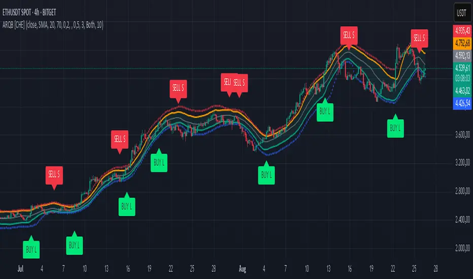
Latched state machines.
Two three-step processes convert levels into “latched” signals that only fire after confirmation and then reset:
* BUY latch:
(1) HLC3 crosses above the median →
(2) the median is rising →
(3) HLC3 prints above the upper (orange) band → BUY latched.
* SELL latch:
(1) HLC3 crosses below the median →
(2) the median is falling →
(3) HLC3 prints below the lower (teal) band → SELL latched.
Labels are drawn on the latch bar, with a FIFO cap to limit clutter. Alerts are available for both the simple band interactions and the latched events. Use “Once per bar close” to avoid intrabar churn.
MTF behavior and repainting.
MTF sourcing uses `lookahead_off`. Quantiles and baselines are computed from completed data only; however, any *intrabar* cross conditions naturally stabilize at close. As with all real-time indicators, values can update during a live bar; prefer bar-close alerts for reliability.
Complexity and parameters.
Each bar sorts a copy of the $N$-length window (practical $N$ values keep this inexpensive). Typical choices: $N=50$–$100$, $q_0=0.15$–$0.25$, $k=2$–$5$, baseline length $L=20$ (if used), adaptation strength $s=0.2$–$0.7$.
Part 2 — Practical Use for Discretionary/Active Traders
What the bands mean in practice.
The teal “buy” band marks the lower tail of the recent distribution; the orange “sell” band marks the upper tail. The median is your dynamic equilibrium. In residual mode, these tails are deviations around trend; in raw mode they are absolute price percentiles. When ATR adaptation is on, tails breathe with regime shifts.
Two core playbooks.
1. Mean-reversion around a stable median.
* Context: The median is flat or gently sloped; band width is relatively tight; instrument is ranging.
* Entry (long): Look for price to probe or close below the buy band and then reclaim it, especially after HLC3 recrosses the median and the median turns up.
* Stops: Place beyond the most recent swing low or $1.0–1.5\times$ ATR(14) below entry.
* Targets: First scale at the median; optional second scale near the opposite band. Trail with the median or an ATR stop.
* Symmetry: Mirror the rules for shorts near the sell band when the median is flat to down.
2. Continuation with latched confirmations.
* Context: A developing trend where you want fewer but cleaner signals.
* Entry (long): Take the latched BUY (3-step confirmation) on close, or on the next bar if you require bar-close validation.
* Invalidation: A close back below the median (or below the lower band in strong trends) negates momentum.
* Exits: Trail under the median for conservative exits or under the teal band for trend-following exits. Consider scaling at structure (prior swing highs) or at a fixed $R$ multiple.
Parameter guidance by timeframe.
* Scalping / LTF (1–5m): $N=30$–$60$, $q_0=0.20$, $k=2$–3, residual mode on, baseline EMA $L=20$, adaptation $s=0.5$–0.7 to handle micro-vol spikes. Expect more signals; rely on latched logic to filter noise.
* Intraday swing (15–60m): $N=60$–$100$, $q_0=0.15$–0.20, $k=3$–4. Residual mode helps but is optional if the instrument trends cleanly. $s=0.3$–0.6.
* Swing / HTF (4H–D): $N=80$–$150$, $q_0=0.10$–0.18, $k=3$–5. Consider `SMA` baseline for smoother residuals and moderate adaptation $s=0.2$–0.4.
Baseline choice.
Use EMA for responsiveness (fast trend shifts) and SMA for stability (smoother residuals). Turning residual mode on is advantageous when price exhibits persistent drift; turning it off is useful when you explicitly want absolute bands.
How to time entries.
Prefer bar-close validation for both band recaptures and latched signals. If you must act intrabar, accept that crosses can “un-cross” before close; compensate with tighter stops or reduced size.
Risk management.
Position size to a fixed fractional risk per trade (e.g., 0.5–1.0% of equity). Define invalidation using structure (swing points) plus ATR. Avoid chasing when distance to the opposite band is small; reward-to-risk degrades rapidly once you are deep inside the distribution.
Combos and filters.
* Pair with a higher-timeframe median slope as a regime filter (trade only in the direction of the HTF median).
* Use band width relative to ATR as a range/trend gauge: unusually narrow bands suggest compression (mean-reversion bias); expanding bands suggest breakout potential (favor latched continuation).
* Volume or session filters (e.g., avoid illiquid hours) can materially improve execution.
Alerts for discretion.
Enable “Cross above Buy Level” / “Cross below Sell Level” for early notices and “Latched BUY/SELL” for conviction entries. Set alerts to “Once per bar close” to avoid noise.
Common pitfalls.
Do not interpret band touches as automatic signals; context matters. A strong trend will often ride the far band (“band walking”) and punish counter-trend fades—use the median slope and latched logic to separate trend from range. Do not oversmooth levels; you will lag breaks. Do not set $q$ too small or too large; extremes reduce statistical meaning and practical distance for stops.
A concise checklist.
1. Is the median flat (range) or sloped (trend)?
2. Is band width expanding or contracting vs ATR?
3. Are we near the tail level aligned with the intended trade?
4. For continuation: did the 3 steps for a latched signal complete?
5. Do stops and targets produce acceptable $R$ (≥1.5–2.0)?
6. Are you trading during liquid hours for the instrument?
Summary. ARQB provides statistically grounded, regime-aware bands and a disciplined, latched confirmation engine. Use the bands as objective context, the median as your equilibrium line, ATR adaptation to stay calibrated across regimes, and the latched logic to time higher-quality discretionary entries.
Disclaimer
No indicator guarantees profits. Adaptive Rolling Quantile Bands is a decision aid; always combine with solid risk management and your own judgment. Backtest, forward test, and size responsibly.
The content provided, including all code and materials, is strictly for educational and informational purposes only. It is not intended as, and should not be interpreted as, financial advice, a recommendation to buy or sell any financial instrument, or an offer of any financial product or service. All strategies, tools, and examples discussed are provided for illustrative purposes to demonstrate coding techniques and the functionality of Pine Script within a trading context.
Any results from strategies or tools provided are hypothetical, and past performance is not indicative of future results. Trading and investing involve high risk, including the potential loss of principal, and may not be suitable for all individuals. Before making any trading decisions, please consult with a qualified financial professional to understand the risks involved.
By using this script, you acknowledge and agree that any trading decisions are made solely at your discretion and risk.
Enhance your trading precision and confidence 🚀
Best regards
Chervolino
Quantiles
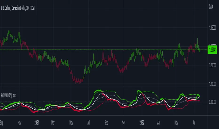
PA-Adaptive MACD w/ Variety Levels [Loxx]PA-Adaptive MACD w/ Variety Levels is a Phase Accumulation Adaptive MACD with both floating and quantile levels. This is tuned for Forex. You'll have to adjust the Phase Accumulation Cycle settings to work for crypto and stock markets.
What is MACD?
Moving average convergence divergence ( MACD ) is a trend-following momentum indicator that shows the relationship between two moving averages of a security’s price. The MACD is calculated by subtracting the 26-period exponential moving average ( EMA ) from the 12-period EMA .
What is the Phase Accumulation Cycle?
The phase accumulation method of computing the dominant cycle is perhaps the easiest to comprehend. In this technique, we measure the phase at each sample by taking the arctangent of the ratio of the quadrature component to the in-phase component. A delta phase is generated by taking the difference of the phase between successive samples. At each sample we can then look backwards, adding up the delta phases.When the sum of the delta phases reaches 360 degrees, we must have passed through one full cycle, on average.The process is repeated for each new sample.
The phase accumulation method of cycle measurement always uses one full cycle’s worth of historical data.This is both an advantage and a disadvantage.The advantage is the lag in obtaining the answer scales directly with the cycle period.That is, the measurement of a short cycle period has less lag than the measurement of a longer cycle period. However, the number of samples used in making the measurement means the averaging period is variable with cycle period. longer averaging reduces the noise level compared to the signal.Therefore, shorter cycle periods necessarily have a higher out- put signal-to-noise ratio.
Included:
Zero-line and signal cross options for bar coloring, signals, and alerts
Alerts
Signals
Loxx's Expanded Source Types
4 moving average types
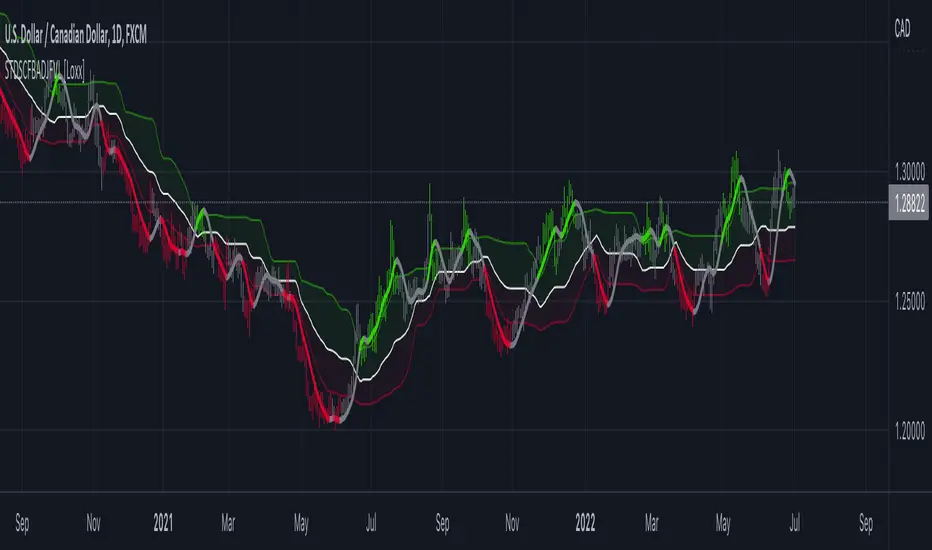
STD-Stepped, CFB-Adaptive Jurik Filter w/ Variety Levels [Loxx]STD-Stepped, CFB-Adaptive Jurik Filter w/ Variety Levels is a Composite Fractal Behavior, single/double Jurik filter with floating boundary levels, alerts, and signals.
What is Composite Fractal Behavior ( CFB )?
All around you mechanisms adjust themselves to their environment. From simple thermostats that react to air temperature to computer chips in modern cars that respond to changes in engine temperature, r.p.m.'s, torque, and throttle position. It was only a matter of time before fast desktop computers applied the mathematics of self-adjustment to systems that trade the financial markets.
Unlike basic systems with fixed formulas, an adaptive system adjusts its own equations. For example, start with a basic channel breakout system that uses the highest closing price of the last N bars as a threshold for detecting breakouts on the up side. An adaptive and improved version of this system would adjust N according to market conditions, such as momentum, price volatility or acceleration.
Since many systems are based directly or indirectly on cycles, another useful measure of market condition is the periodic length of a price chart's dominant cycle, (DC), that cycle with the greatest influence on price action.
The utility of this new DC measure was noted by author Murray Ruggiero in the January '96 issue of Futures Magazine. In it. Mr. Ruggiero used it to adaptive adjust the value of N in a channel breakout system. He then simulated trading 15 years of D-Mark futures in order to compare its performance to a similar system that had a fixed optimal value of N. The adaptive version produced 20% more profit!
This DC index utilized the popular MESA algorithm (a formulation by John Ehlers adapted from Burg's maximum entropy algorithm, MEM). Unfortunately, the DC approach is problematic when the market has no real dominant cycle momentum, because the mathematics will produce a value whether or not one actually exists! Therefore, we developed a proprietary indicator that does not presuppose the presence of market cycles. It's called CFB (Composite Fractal Behavior) and it works well whether or not the market is cyclic.
CFB examines price action for a particular fractal pattern, categorizes them by size, and then outputs a composite fractal size index. This index is smooth, timely and accurate
Essentially, CFB reveals the length of the market's trending action time frame. Long trending activity produces a large CFB index and short choppy action produces a small index value. Investors have found many applications for CFB which involve scaling other existing technical indicators adaptively, on a bar-to-bar basis.
What is Jurik Volty used in the Juirk Filter?
One of the lesser known qualities of Juirk smoothing is that the Jurik smoothing process is adaptive. "Jurik Volty" (a sort of market volatility ) is what makes Jurik smoothing adaptive. The Jurik Volty calculation can be used as both a standalone indicator and to smooth other indicators that you wish to make adaptive.
What is the Jurik Moving Average?
Have you noticed how moving averages add some lag (delay) to your signals? ... especially when price gaps up or down in a big move, and you are waiting for your moving average to catch up? Wait no more! JMA eliminates this problem forever and gives you the best of both worlds: low lag and smooth lines.
Ideally, you would like a filtered signal to be both smooth and lag-free. Lag causes delays in your trades, and increasing lag in your indicators typically result in lower profits. In other words, late comers get what's left on the table after the feast has already begun.
Included:
-Color bars
-Color background
-Color trend
-Color deadzones
-Show signals
-Long/short alerts
-ATR and quantile based levels
Weighted Harrell-Davis Quantile Estimator with AbsoluteDeviation
QUANTILE ESTIMATORS
Weighted Harrell-Davis Quantile Estimator with Absolute Deviation Fences.
DISCLAIMER:
The Following indicator/code IS NOT intended to be a formal investment advice or recommendation by the author, nor should be construed as such. Users will be fully responsible by their use regarding their own trading vehicles/assets.
The following indicator was made for NON LUCRATIVE ACTIVITIES and must remain as is, following TradingView's regulations. Use of indicator and their code are published for work and knowledge sharing. All access granted over it, their use, copy or re-use should mention authorship(s) and origin(s).
WARNING NOTICE!
THE INCLUDED FUNCTION MUST BE CONSIDERED FOR TESTING. The models included in the indicator have been taken from open sources on the web and some of them has been modified by the author, problems could occur at diverse data sceneries, compiler version, or any other externality.
Purpose:
Weighted Quantiles or <> are quite difficult to find on must systems, also it's non-weighted approach are rarely used to estimate the location parameter of price distribution WICH IS NOT NORMAL, all this in favour of it's non-robust counterpart, the Arithmetic rolling Mean or <> and it's weighted variants like the WMA, VWAP, etc.
Also, a big drawback from this is that must statistics derived from Normal-Distribution parameter location (the Mean) definitely will not fit for an efficient, nor robust estimation for price distributions, so their moments like the standard deviation, kurtosis, skewness, etc. will not be the better tools to build derived algorithms or technical indicators among price/volume.
In an effort searching better statistical tools for price distributions, I found the excellent work of Andrey Akinshin that took me to port some of their Math research contributions for the compute benchmarking field , and bring it here at the TradingView ecosystem to take a shot at the price distribution crazy fields. For a better detail of what the weighted Harrell-Davis Quantile Estimator can do, who better than drink directly from the source at References:
References:
Weighted Quantile Estimators.
DoubleMAD outlier detector based on the Harrell-Davis quantile estimator.
Unbiased median absolute deviation based on the Harrell-Davis quantile estimator.
Quantile confidence intervals for weighted samples.
Licensing:
This work is licensed under a Attribution-NonCommercial-ShareAlike 4.0 International Copyright (c) 2021 (CC BY-NC-SA 4.0)
Copyright's & Mentions:
The Gamma Functions & Beta Probability Density Functions C# implementations by the Math.NET Numerics, part of the Math.NET Project.
The Regularized Incomplete (Left) Beta Function C# implementation by the SAMTools, htslib project.
The Weighted Harrell-Davis Quantile estimator ; C# & R implementations by Andrey Akinshin.
External PineScript code, methods, support & consultancy by @PineCoders staff with special mention for:
+ "ma sorter ('sort by array' example)- JD" by @Duyck.
+ Porting, mods, compilation and debugging for this script by @XeL_Arjona for the TradingView's @PineCoders community.