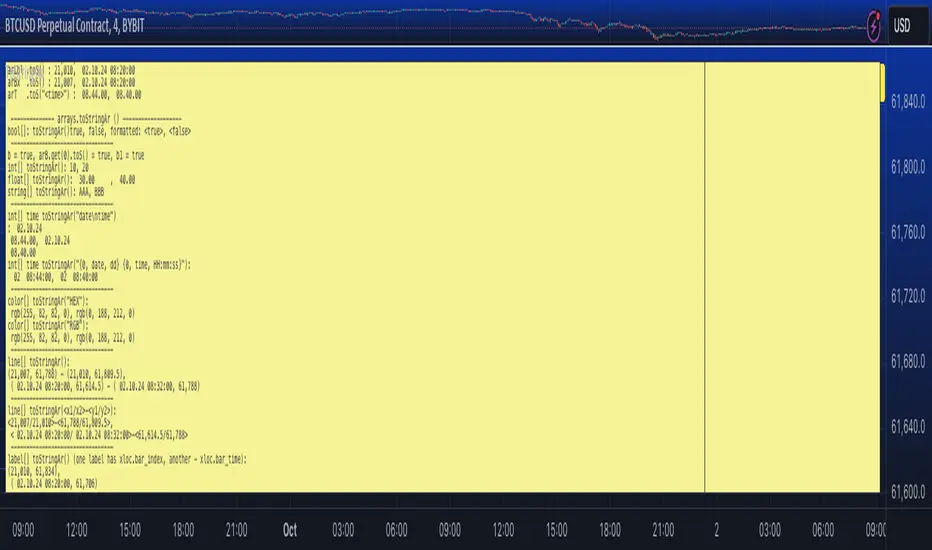
ToStringAr█ OVERVIEW
Contains to string conversion methods arrays of int/float/bool/string/line/label/box types
- toS() - method works like array.join() with more flexibility and
- toStringAr() - converts array to string on a per item basis and returns the resulting string array
Conversion of each item to string is made using toS() function from moebius1977/ToS/1 library.
█ GENERAL DESCRIPTION OF LIBRARY FUNCTIONS
All toS(array) methods have same parameters. The only difference will be in format parameter as explained below.
method toS(this, index_from, index_to, separator, showIDs, format, truncate_left, size_limit, nz)
Like array.join() but with string length limit. Joins elements into readable string (length capped at 4000, truncating the end or beg)
Parameters:
this (array) : array to be converted to string
index_from (int) : index_from (int) (Optional) Start from this id (starting from 0, in insertion order). If omitted - start from the first item.
index_to (int) : index_to (int) (Optional) End with this pair (inclusive, in insertion order). If omitted - to last item.
separator (string) : separator (string) (Optional) String to be inserted between pairs. Default: `", "`
showIDs (bool) : showIDs (bool) (Optional) If true item's id is added in the form `id: value`.
format (string) : format (string) (Optional) Format string fo toS(). If omitted default format is used depending in the type.
truncate_left (bool) : truncate_left (bool) (Optional) Truncate from left or right. Default: false.
size_limit (int) : size_limit (int) (Optional) Max output string length. Default: 4000.
nz (string) : nz (string) (Optional) A string used to represent na (na values are substituted with this string).
format parameter depends on the type:
For toS(bool/int/float ...) format parameter works in the same way as `str.format()` (i.e. you can use same format strings as with `str.format()` with `{0}` as a placeholder for the value) with some shorthand "format" options available:
--- number ---
- "" => "{0}"
- "number" => "{0}"
- "0" => "{0, number, 0 }"
- "0.0" => "{0, number, 0.0 }"
- "0.00" => "{0, number, 0.00 }"
- "0.000" => "{0, number, 0.000 }"
- "0.0000" => "{0, number, 0.0000 }"
- "0.00000" => "{0, number, 0.00000 }"
- "0.000000" => "{0, number, 0.000000 }"
- "0.0000000" => "{0, number, 0.0000000}"
--- date ---
- "... ... " in any place is substituted with "{0, date, dd.MM.YY}" (e.g. " " results in "{0, date, dd.MM.YY\} {0, time, HH.mm.ss}")
- "date" => "{0, date, dd.MM.YY}"
- "date : time" => "{0, date, dd.MM.YY} : {0, time, HH.mm.ss}"
- "dd.MM" => "{0, date, dd:MM}"
- "dd" => "{0, date, dd}"
--- time ---
- "... ... " in any place is substituted with "{0, time, HH.mm.ss}" (e.g. " " results in "{0, date, dd.MM.YY\} {0, time, HH.mm.ss}")
- "time" => "{0, time, HH:mm:ss}"
- "HH:mm" => "{0, time, HH:mm}"
- "mm:ss" => "{0, time, mm:ss}"
- "date time" => "{0, date, dd.MM.YY\} {0, time, HH.mm.ss}"
- "date, time" => "{0, date, dd.MM.YY\}, {0, time, HH.mm.ss}"
- "date,time" => "{0, date, dd.MM.YY\},{0, time, HH.mm.ss}"
- "date\ntime" => "{0, date, dd.MM.YY\}\n{0, time, HH.mm.ss}"
For toS(line ...):
format (string) : (string) (Optional) Use `x1` as placeholder for `x1` and so on. E.g. default format is `"(x1, y1) - (x2, y2)"`.
For toS(label ...) :
format (string) : (string) (Optional) Use `x1` as placeholder for `x`, `y1 - for `y` and `txt` for label's text. E.g. default format is `(x1, y1): "txt"` if ptint_text is true and `(x1, y1)` if false.
For toS(box ... ) :
format (string) : (string) (Optional) Use `x1` as placeholder for `x`, `y1 - for `y` etc. E.g. default format is "(x1, y1) - (x2, y2)".
For toS(color] ... ) :
format (string) : (string) (Optional) Options are "HEX" (e.g. "#FFFFFF33") or "RGB" (e.g. "rgb(122,122,122,23)"). Default is "HEX".
All toStringAr() methods just convert each item to string using toS with same format options as described above.
Parameters:
arr (array) : Array to be converted to a string array.
format (string) : Format string.
nz (string) : Placeholder for na items.
█ FULL OF FUNCTIONS AND PARAMETERS
Library "ToStringAr"
Contains toString/toS conversion methods for int/float/bool/string/line/label/box and arrays and matrices thereof. Also contains a string wraping function.
method toS(this, index_from, index_to, separator, showIDs, format, truncate_left, size_limit, nz)
Namespace types: array
Parameters:
this (array)
index_from (int)
index_to (int)
separator (string)
showIDs (bool)
format (string)
truncate_left (bool)
size_limit (int)
nz (string)
method toS(this, index_from, index_to, separator, showIDs, format, truncate_left, size_limit, nz)
Namespace types: array
Parameters:
this (array)
index_from (int)
index_to (int)
separator (string)
showIDs (bool)
format (string)
truncate_left (bool)
size_limit (int)
nz (string)
method toS(this, index_from, index_to, separator, showIDs, format, truncate_left, size_limit, nz)
Namespace types: array
Parameters:
this (array)
index_from (int)
index_to (int)
separator (string)
showIDs (bool)
format (string)
truncate_left (bool)
size_limit (int)
nz (string)
method toS(this, index_from, index_to, separator, showIDs, format, truncate_left, size_limit, nz)
Namespace types: array
Parameters:
this (array)
index_from (int)
index_to (int)
separator (string)
showIDs (bool)
format (string)
truncate_left (bool)
size_limit (int)
nz (string)
method toS(this, index_from, index_to, separator, showIDs, format, truncate_left, size_limit, nz)
Namespace types: array
Parameters:
this (array)
index_from (int)
index_to (int)
separator (string)
showIDs (bool)
format (string)
truncate_left (bool)
size_limit (int)
nz (string)
method toS(this, index_from, index_to, separator, showIDs, format, truncate_left, size_limit, nz)
Namespace types: array
Parameters:
this (array)
index_from (int)
index_to (int)
separator (string)
showIDs (bool)
format (string)
truncate_left (bool)
size_limit (int)
nz (string)
method toS(this, index_from, index_to, separator, showIDs, format, truncate_left, size_limit, nz)
Namespace types: array
Parameters:
this (array)
index_from (int)
index_to (int)
separator (string)
showIDs (bool)
format (string)
truncate_left (bool)
size_limit (int)
nz (string)
method toS(this, index_from, index_to, separator, showIDs, format, truncate_left, size_limit, nz)
Namespace types: array
Parameters:
this (array)
index_from (int)
index_to (int)
separator (string)
showIDs (bool)
format (string)
truncate_left (bool)
size_limit (int)
nz (string)
method toStringAr(arr, format, nz)
Namespace types: array
Parameters:
arr (array)
format (string)
nz (string)
method toStringAr(arr, format, nz)
Namespace types: array
Parameters:
arr (array)
format (string)
nz (string)
method toStringAr(arr, format, nz)
Namespace types: array
Parameters:
arr (array)
format (string)
nz (string)
method toStringAr(arr, format, nz)
Namespace types: array
Parameters:
arr (array)
format (string)
nz (string)
method toStringAr(arr, format, nz)
Namespace types: array
Parameters:
arr (array)
format (string)
nz (string)
method toStringAr(arr, format, nz)
Namespace types: array
Parameters:
arr (array)
format (string)
nz (string)
method toStringAr(arr, format, nz)
Namespace types: array
Parameters:
arr (array)
format (string)
nz (string)
method toStringAr(arr, format, nz)
Namespace types: array
Parameters:
arr (array)
format (string)
nz (string)
在腳本中搜尋"上证指数4000是什么时候"
Multi-Exchange Volume (30 Tickers) by kurtsmock + BV + rVolauthor: kurtsmock
Fully Customizable ticker set. Up to 30 Tickers. Bitcoin set as default.
-- IMPORTANT NOTE: --
30 Exchanges are a lot. It can take a while to load. You can fully customize this indicator to your liking. Here's how:
1. Load indicator
2. Open Settings
3. Uncheck the switch box for exchanges you want unincluded
4. At the bottom of the settings menu click "Defaults" and hit "Save as Default"
5. To turn them all back on, hit "Reset Settings" in that same "Defaults" menu and click "Save as Default" again.
Also, you don't have to use this with Bitcoin. This works with any asset, just change the ticker in the settings.
There's a lot going on with this indicator so the following is descriptions and instructions to help you better understand what's going on here. Thanks!
Goal:
- To provide a mechanism for assets on multiple exchanges to have their volume evaluated together
Edge:
- Having better and more complete volume information
Notes:
- The Default Exchanges for this indicator are highest volume bitcoin exchanges, but may contain "fake volume"
- Indicator is set for Bitcoin by default. However, you can change the tickers to reflect any asset you want
////// rVol //////
Goal:
- To understand how much volume is being executed relative to the same candle on previous days/periods
Edge:
- Higher rVol implies higher volatility and market interest.
- High rVol = higher than average volume . Markets move on volume so higher than average volume indicates increased market activity/volatility
- rVol is an indirect measure of active or anticipated volatility
Definitions:
- rVol: The volume of a period compared to the Average Volume of that same period in past sessions
- Important to note it does NOT add up the last 10 (default) candles, but rather the last 10 candles at session intervals.
- Example:
-- On a Tuesday, 1h chart it will add up the last ten Tuesday, 9:00 am candles, not including the current, active candle.
-- It then averages those lookback candles.
-- It then plots the percentage relationship between the most recent candle and the average of the lookback candles
-- Avg Vol of Lookback candles = 5000,
-- Volume of most recent candle = 4000: Output = rVol = 80:
-- Volume of most recent candle was 80% of the average volume in the 9 am time period of the last ten Tuesdays in the 9 am, 1h period
Notes:
- rVol does not add current candle volume into lookback sum. So, you set lookback to be: (not including the current day)
- rVol is on a switch. So, if you want to see rVol instead of volume, hit the switch in the settings
- If you want to see both, load 2 instances of the indicator.
////// Better-er Volume //////
Goal:
To Identify:
- When a candle closes at the highest volume * range relative to the lookback period and close > open
- When a candle closes at the highest volume * range relative to the lookback period and close < open
- When a candle closes at the highest volume / price relative to the lookback period
Edge:
- Identifies beginnings of price expansion, climax of price expansion, breakouts, pivots, and take profit points on the volume chart
Notes:
- Based generally on Barry Taylor's "Better Volume" indicator and ideas from Pascal Willain's book "Value in Time."
- Better-er Volume rules are applied to both Total Volume or rVol.
-- When rVol is displayed Better-er Volume is applied to rVol
-- When Total Volume is displayed Better-er Volume is applied to Total Volume
// Plot Key: //
Green Triangle Up = Often marks the beginning and/or end of price expansion to the upside
Red Triangle Up = Often marks the beginning and/or end of price expansion to the downside
Yellow Square = High Volume but Tight Range. Implies a Battle of Bulls and Bears. High Liquidity area. Provided Liquidity is not enough to move price. Thick Limit Order Book.
Purple Triangle Up or Down = Implies high market participation. Typically at the end of expansion when very significant s/r is hit
category: volume Volatility
tags: Volume rVol relativevolume Bitcoin cryptocurrency bettervolume
Many More Volume Indicators Coming Out Soon!

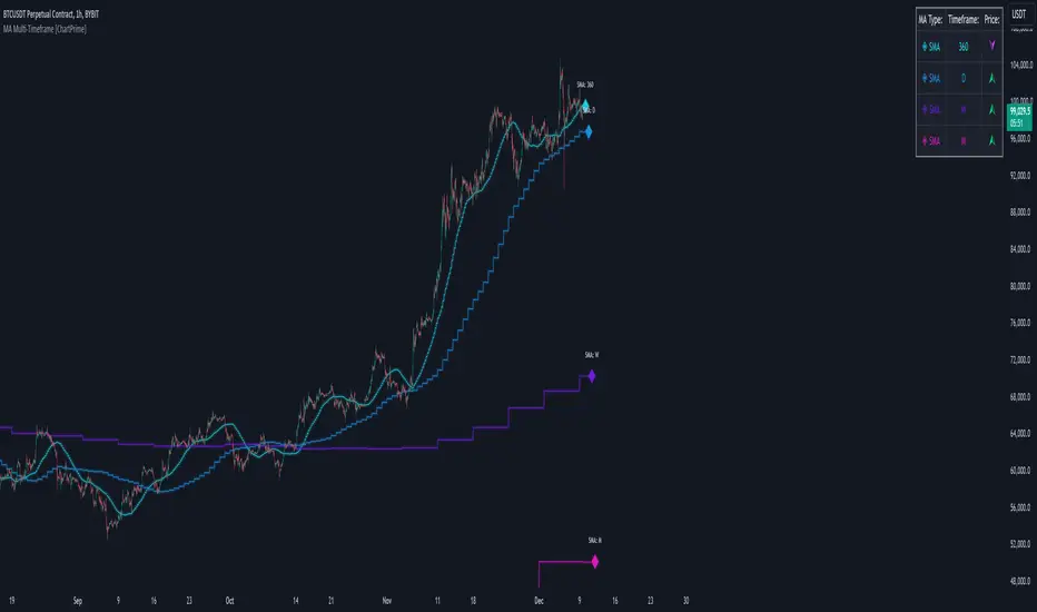
MA Multi-Timeframe [ChartPrime]The MA Multi-Timeframe indicator is designed to provide multi-timeframe moving averages (MAs) for better trend analysis across different periods. This tool allows traders to monitor up to four different MAs on a single chart, each coming from a selectable timeframe and type (SMA, EMA, SMMA, WMA, VWMA). The indicator helps traders gauge both short-term and long-term price trends, allowing for a clearer understanding of market dynamics.
⯁ KEY FEATURES AND HOW TO USE
⯌ Multi-Timeframe Moving Averages :
The indicator allows traders to select up to four MAs, each from different timeframes. These timeframes can be set in the input settings (e.g., Daily, Weekly, Monthly), and each moving average can be displayed with its corresponding timeframe label directly on the chart.
Example of different timeframes for MAs:
⯌ Moving Average Types :
Users can choose from several types of moving averages, including SMA, EMA, SMMA, WMA, and VWMA, making the indicator adaptable to different strategies and market conditions. This flexibility allows traders to tailor the MAs to their preference.
Example of different types of MAs:
⯌ Dashboard Display :
The indicator includes a built-in dashboard that shows each MA, its timeframe, and whether the price is currently above or below that MA. This dashboard provides a quick overview of the trend across different timeframes, allowing traders to determine whether the overall trend is up or down.
Example of trend overview via the dashboard:
⯌ Polyline Representation :
Each MA is plotted using polylines to avoid plot functions and create a curves across up to 4000 bars back, ensuring that historical data is visualized clearly for a deeper analysis of how the price interacts with these levels over time.
if barstate.islast
for i = 0 to 4000
cp.push(chart.point.from_index(bar_index , ma ))
polyline.delete(polyline.new(cp, curved = false, line_color = color, line_style = style) )
Example of polylines for moving averages:
⯌ Customization Options :
Traders can customize the length of the MAs for all timeframes using a single input. The color, style (solid, dashed, dotted) of each moving average are also customizable, giving users full control over the visual appearance of the indicator on their chart.
Example of custom MA styles:
⯁ USER INPUTS
MA Type : Select the type of moving average for each timeframe (SMA, EMA, SMMA, WMA, VWMA).
Timeframe : Choose the timeframe for each moving average (e.g., Daily, Weekly, Monthly).
MA Length : Set the length for the moving averages, which will be applied to all four MAs.
Line Style : Customize the style of each MA line (solid, dashed, or dotted).
Colors : Set the color for each MA for better visual distinction.
⯁ CONCLUSION
The MA Multi-Timeframe indicator is a versatile and powerful tool for traders looking to monitor price trends across multiple timeframes with different types of moving averages. The dashboard simplifies trend identification, while the customizable options make it easy to adapt to individual trading strategies. Whether you're analyzing short-term price movements or long-term trends, this indicator offers a comprehensive solution for tracking market direction.
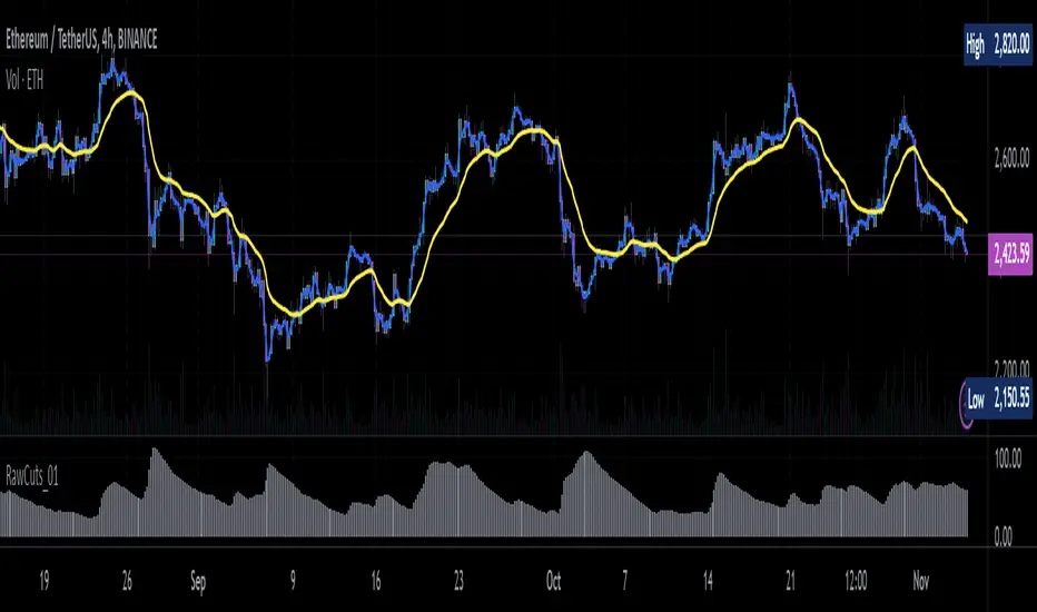
RawCuts_01Library "RawCuts_01"
A collection of functions by:
mutantdog
The majority of these are used within published projects, some useful variants have been included here aswell.
This is volume one consisting mainly of smaller functions, predominantly the filters and standard deviations from Weight Gain 4000.
Also included at the bottom are various snippets of related code for demonstration. These can be copied and adjusted according to your needs.
A full up-to-date table of contents is located at the top of the main script.
WEIGHT GAIN FILTERS
A collection of moving average type filters with adjustable volume weighting.
Based upon the two most common methods of volume weighting.
'Simple' uses the standard method in which a basic VWMA is analogous to SMA.
'Elastic' uses exponential method found in EVWMA which is analogous to RMA.
Volume weighting is applied according to an exponent multiplier of input volume.
0 >> volume^0 (unweighted), 1 >> volume^1 (fully weighted), use float values for intermediate weighting.
Additional volume filter switch for smoothing of outlier events.
DIVA MODULAR DEVIATIONS
A small collection of standard and absolute deviations.
Includes the weightgain functionality as above.
Basic modular functionality for more creative uses.
Optional input (ct) for external central tendency (aka: estimator).
Can be assigned to alternative filter or any float value. Will default to internal filter when no ct input is received.
Some other useful or related functions included at the bottom along with basic demonstration use.
weightgain_sma(src, len, xVol, fVol)
Simple Moving Average (SMA): Weight Gain (Simple Volume).
Parameters:
src (float) : Source input.
len (int) : Length (number of bars).
xVol (float) : Volume exponent multiplier (0 = unweighted, 1 = fully weighted).
fVol (bool) : Volume smoothing filter.
Returns: Standard Simple Moving Average with Simple Weight Gain applied.
weightgain_hsma(src, len, xVol, fVol)
Harmonic Simple Moving Average (hSMA): Weight Gain (Simple Volume).
Parameters:
src (float) : Source input.
len (int) : Length (number of bars).
xVol (float) : Volume exponent multiplier (0 = unweighted, 1 = fully weighted).
fVol (bool) : Volume smoothing filter.
Returns: Harmonic Simple Moving Average with Simple Weight Gain applied.
weightgain_gsma(src, len, xVol, fVol)
Geometric Simple Moving Average (gSMA): Weight Gain (Simple Volume).
Parameters:
src (float) : Source input.
len (int) : Length (number of bars).
xVol (float) : Volume exponent multiplier (0 = unweighted, 1 = fully weighted).
fVol (bool) : Volume smoothing filter.
Returns: Geometric Simple Moving Average with Simple Weight Gain applied.
weightgain_wma(src, len, xVol, fVol)
Linear Weighted Moving Average (WMA): Weight Gain (Simple Volume).
Parameters:
src (float) : Source input.
len (int) : Length (number of bars).
xVol (float) : Volume exponent multiplier (0 = unweighted, 1 = fully weighted).
fVol (bool) : Volume smoothing filter.
Returns: Basic Linear Weighted Moving Average with Simple Weight Gain applied.
weightgain_hma(src, len, xVol, fVol)
Hull Moving Average (HMA): Weight Gain (Simple Volume).
Parameters:
src (float) : Source input.
len (int) : Length (number of bars).
xVol (float) : Volume exponent multiplier (0 = unweighted, 1 = fully weighted).
fVol (bool) : Volume smoothing filter.
Returns: Basic Hull Moving Average with Simple Weight Gain applied.
diva_sd_sma(src, len, xVol, fVol, ct)
Standard Deviation (SD SMA): Diva / Weight Gain (Simple Volume)
Parameters:
src (float) : Source input.
len (int) : Length (number of bars).
xVol (float) : Volume exponent multiplier (0 = unweighted, 1 = fully weighted).
fVol (bool) : Volume smoothing filter.
ct (float) : Central tendency (optional, na = bypass). Internal: weightgain_sma().
Returns:
diva_sd_wma(src, len, xVol, fVol, ct)
Standard Deviation (SD WMA): Diva / Weight Gain (Simple Volume).
Parameters:
src (float) : Source input.
len (int) : Length (number of bars).
xVol (float) : Volume exponent multiplier (0 = unweighted, 1 = fully weighted).
fVol (bool) : Volume smoothing filter.
ct (float) : Central tendency (optional, na = bypass). Internal: weightgain_wma().
Returns:
diva_aad_sma(src, len, xVol, fVol, ct)
Average Absolute Deviation (AAD SMA): Diva / Weight Gain (Simple Volume).
Parameters:
src (float) : Source input.
len (int) : Length (number of bars).
xVol (float) : Volume exponent multiplier (0 = unweighted, 1 = fully weighted).
fVol (bool) : Volume smoothing filter.
ct (float) : Central tendency (optional, na = bypass). Internal: weightgain_sma().
Returns:
diva_aad_wma(src, len, xVol, fVol, ct)
Average Absolute Deviation (AAD WMA): Diva / Weight Gain (Simple Volume) .
Parameters:
src (float) : Source input.
len (int) : Length (number of bars).
xVol (float) : Volume exponent multiplier (0 = unweighted, 1 = fully weighted).
fVol (bool) : Volume smoothing filter.
ct (float) : Central tendency (optional, na = bypass). Internal: weightgain_wma().
Returns:
weightgain_ema(src, len, xVol, fVol)
Exponential Moving Average (EMA): Weight Gain (Elastic Volume).
Parameters:
src (float) : Source input.
len (int) : Length (number of bars).
xVol (float) : Volume exponent multiplier (0 = unweighted, 1 = fully weighted).
fVol (bool) : Volume smoothing filter.
Returns: Exponential Moving Average with Elastic Weight Gain applied.
weightgain_dema(src, len, xVol, fVol)
Double Exponential Moving Average (DEMA): Weight Gain (Elastic Volume).
Parameters:
src (float) : Source input.
len (int) : Length (number of bars).
xVol (float) : Volume exponent multiplier (0 = unweighted, 1 = fully weighted).
fVol (bool) : Volume smoothing filter.
Returns: Double Exponential Moving Average with Elastic Weight Gain applied.
weightgain_tema(src, len, xVol, fVol)
Triple Exponential Moving Average (TEMA): Weight Gain (Elastic Volume).
Parameters:
src (float) : Source input.
len (int) : Length (number of bars).
xVol (float) : Volume exponent multiplier (0 = unweighted, 1 = fully weighted).
fVol (bool) : Volume smoothing filter.
Returns: Triple Exponential Moving Average with Elastic Weight Gain applied.
weightgain_rma(src, len, xVol, fVol)
Rolling Moving Average (RMA): Weight Gain (Elastic Volume).
Parameters:
src (float) : Source input.
len (int) : Length (number of bars).
xVol (float) : Volume exponent multiplier (0 = unweighted, 1 = fully weighted).
fVol (bool) : Volume smoothing filter.
Returns: Rolling Moving Average with Elastic Weight Gain applied.
weightgain_drma(src, len, xVol, fVol)
Double Rolling Moving Average (DRMA): Weight Gain (Elastic Volume).
Parameters:
src (float) : Source input.
len (int) : Length (number of bars).
xVol (float) : Volume exponent multiplier (0 = unweighted, 1 = fully weighted).
fVol (bool) : Volume smoothing filter.
Returns: Double Rolling Moving Average with Elastic Weight Gain applied.
weightgain_trma(src, len, xVol, fVol)
Triple Rolling Moving Average (TRMA): Weight Gain (Elastic Volume).
Parameters:
src (float) : Source input.
len (int) : Length (number of bars).
xVol (float) : Volume exponent multiplier (0 = unweighted, 1 = fully weighted).
fVol (bool) : Volume smoothing filter.
Returns: Triple Rolling Moving Average with Elastic Weight Gain applied.
diva_sd_ema(src, len, xVol, fVol, ct)
Standard Deviation (SD EMA): Diva / Weight Gain: (Elastic Volume).
Parameters:
src (float) : Source input.
len (int) : Length (number of bars).
xVol (float) : Volume exponent multiplier (0 = unweighted, 1 = fully weighted).
fVol (bool) : Volume smoothing filter.
ct (float) : Central tendency (optional, na = bypass). Internal: weightgain_ema().
Returns:
diva_sd_rma(src, len, xVol, fVol, ct)
Standard Deviation (SD RMA): Diva / Weight Gain: (Elastic Volume).
Parameters:
src (float) : Source input.
len (int) : Length (number of bars).
xVol (float) : Volume exponent multiplier (0 = unweighted, 1 = fully weighted).
fVol (bool) : Volume smoothing filter.
ct (float) : Central tendency (optional, na = bypass). Internal: weightgain_rma().
Returns:
weightgain_vidya_rma(src, len, xVol, fVol)
VIDYA v1 RMA base (VIDYA-RMA): Weight Gain (Elastic Volume).
Parameters:
src (float) : Source input.
len (int) : Length (number of bars).
xVol (float) : Volume exponent multiplier (0 = unweighted, 1 = fully weighted).
fVol (bool) : Volume smoothing filter.
Returns: VIDYA v1, RMA base with Elastic Weight Gain applied.
weightgain_vidya_ema(src, len, xVol, fVol)
VIDYA v1 EMA base (VIDYA-EMA): Weight Gain (Elastic Volume).
Parameters:
src (float) : Source input.
len (int) : Length (number of bars).
xVol (float) : Volume exponent multiplier (0 = unweighted, 1 = fully weighted).
fVol (bool) : Volume smoothing filter.
Returns: VIDYA v1, EMA base with Elastic Weight Gain applied.
diva_sd_vidya_rma(src, len, xVol, fVol, ct)
Standard Deviation (SD VIDYA-RMA): Diva / Weight Gain: (Elastic Volume).
Parameters:
src (float) : Source input.
len (int) : Length (number of bars).
xVol (float) : Volume exponent multiplier (0 = unweighted, 1 = fully weighted).
fVol (bool) : Volume smoothing filter.
ct (float) : Central tendency (optional, na = bypass). Internal: weightgain_vidya_rma().
Returns:
diva_sd_vidya_ema(src, len, xVol, fVol, ct)
Standard Deviation (SD VIDYA-EMA): Diva / Weight Gain: (Elastic Volume).
Parameters:
src (float) : Source input.
len (int) : Length (number of bars).
xVol (float) : Volume exponent multiplier (0 = unweighted, 1 = fully weighted).
fVol (bool) : Volume smoothing filter.
ct (float) : Central tendency (optional, na = bypass). Internal: weightgain_vidya_ema().
Returns:
weightgain_sema(src, len, xVol, fVol)
Parameters:
src (float)
len (simple int)
xVol (float)
fVol (bool)
diva_sd_sema(src, len, xVol, fVol)
Parameters:
src (float)
len (simple int)
xVol (float)
fVol (bool)
diva_mad_mm(src, len, ct)
Median Absolute Deviation (MAD MM): Diva (no volume weighting).
Parameters:
src (float) : Source input.
len (int) : Length (number of bars).
ct (float) : Central tendency (optional, na = bypass). Internal: ta.median()
Returns:
source_switch(slct, aux1, aux2, aux3, aux4)
Custom Source Selector/Switch function. Features standard & custom 'weighted' sources with additional aux inputs.
Parameters:
slct (string) : Choose from custom set of string values.
aux1 (float) : Additional input for user-defined source, eg: standard input.source(). Optional, use na to bypass.
aux2 (float) : Additional input for user-defined source, eg: standard input.source(). Optional, use na to bypass.
aux3 (float) : Additional input for user-defined source, eg: standard input.source(). Optional, use na to bypass.
aux4 (float) : Additional input for user-defined source, eg: standard input.source(). Optional, use na to bypass.
Returns: Float value, to be used as src input for other functions.
colour_gradient_ma_div(ma1, ma2, div, bull, bear, mid, mult)
Colour Gradient for plot fill between two moving averages etc, with seperate bull/bear and divergence strength.
Parameters:
ma1 (float) : Input for fast moving average (eg: bullish when above ma2).
ma2 (float) : Input for slow moving average (eg: bullish when below ma1).
div (float) : Input deviation/divergence value used to calculate strength of colour.
bull (color) : Colour when ma1 above ma2.
bear (color) : Colour when ma1 below ma2.
mid (color) : Neutral colour when ma1 = ma2.
mult (int) : Opacity multiplier. 100 = maximum, 0 = transparent.
Returns: Colour with transparency (according to specified inputs)
ATR Percentage of PriceThis indicator takes the standard ATR and expresses it as a percentage of the OHLC4 price. This has the advantage of normalising the ATR value across the history of an asset. For example, an ATR of value 20 when the price is 2000 actually has a very different meaning when the price rises to 4000. The ATR may be the same value but actually the volatility it represents has halved.
I also add an SMA to the value and a histogram which shows the difference between the two. Positive values mean that volatility is expanding while negative values mean volatility is contracting.

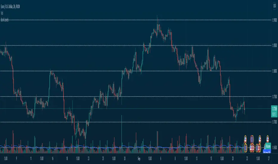
Bank Levels - Psychological Levels - Bitcoin, Indices, ForexThis got removed so I'm publishing it again.
What it is:
- This script draws in levels refereed to as bank levels. They are basically psychological/even numbers(40000, 45000, 150, 1850..)
Why doesn't it work on some charts?
- Each pair has a different tick value. You will have to edit the code to make it work on certain pairs. It's pretty simple, take a look.
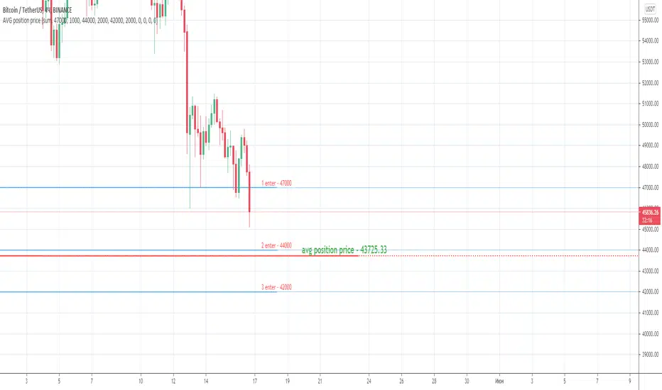
AVG position priceThis is a simple script that can show the average price of your position.
You can use up to 5 levels of averaging.
Use sum or amount setting - default - amount - you must enter price and amount - for example, your first purchase was - 0.1 bitcoin at 47000, second one - 0.2 btc at 45000 , so you must use this numbers.
Or you can choose "sum" - For example, you want to see what the average price of your position will be if you buy bitcoin for $ 1000 at the level of 47000 and later buy in addition for 2000 at the level of 46000 and another 2000 at the level of 43000.
__________________________________
Скрипт, показывающий среднюю точку входа в позицию.
В настройках необходимо выбрать:
- "amount" если вы знаете точное количество приобретаемого актива - например покупаете 0.1 биткоина на уровне 47000, далее докупаете 0.2 биткоина на 45к итд.
- "sum" если расчет идет исходя из суммы покупки - например взяли на 1к по 47000, дальше на 2к по 45к и еще на 2к по 40000
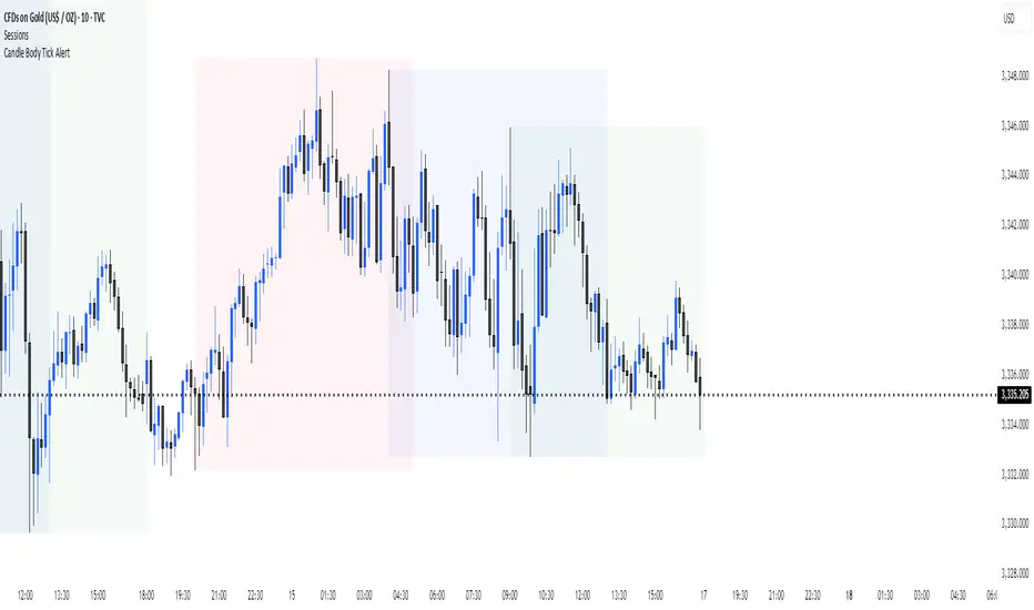
Candle Body Size AlertThis indicator monitors the body size of each candle (close minus open, ignoring wicks) and compares it to a user-defined threshold measured in ticks. If the candle body exceeds the threshold, the indicator triggers an alert condition at the close of the candle.
Features:
1. Adjustable threshold in ticks (default: 4000)
2. Adjustable timeframe (or use chart timeframe)
3. Alerts only at candle close (no intrabar signals)
Use Case:
Designed for traders who want to be notified when unusually large candles form, helping to identify strong momentum moves or volatility spikes.
AWR_8DLRC1. Overview and Objective
The AWR_8DLRC indicator is designed to display multiple dynamic channels directly on your chart (with the overlay enabled). It creates dynamic envelopes based on a regression-like approach combined with a volatility measure derived from the root mean square error (RMSE). These channels can help identify support and resistance areas, overbought/oversold conditions, or even potential trend reversals by providing several layers of analysis using different multipliers and timeframes.
2. Input Parameters
Source and Multiplier
The indicator uses the closing price (close) as its default data source.
A floating-point parameter mult (default value: 3.0) is available. This multiplier is primarily used for channel 5, while other channels employ fixed multipliers (1, 2, or 3) to generate different sensitivity levels.
Channel Lengths
Several channels are calculated with distinct lookback lengths:
Channel 5: Uses a length of 1000 periods (its plot is commented out in the code, so it is not displayed by default).
Channel 6: Uses a length of 2000 periods.
Channel 7: Uses a length of 3000 periods.
Channel 8: Uses a length of 4000 periods.
Custom Colors and Transparencies
Each channel (or group of channels) can be customized with specific colors and transparency settings. For example, channel 6 uses a light yellow tone, channel 7 is red, and channel 8 is white.
Additionally, specific fill colors are defined for the shaded areas between the upper and lower lines of some channels, enhancing visual clarity.
3. Channel Calculation Mechanism
At the heart of the indicator is the function f_calcChannel(), which takes as input:
A data source (_src),
A period (_length), and
A multiplier (_mult).
The calculation process comprises several key steps:
Moving Averages Calculation
The function computes both a weighted moving average (WMA) and a simple moving average (SMA) over the defined length.
Baseline Determination
It then combines these averages into two values (A and B) using linear formulas (e.g., A = 4*b - 3*a and B = 3*a - 2*b). These values help to establish a baseline that represents the central trend during the lookback period.
Slope and Deviation Calculation
A slope (m) is calculated based on the difference between A and B.
The function iterates over the period, measuring the squared deviation between the actual data point and a corresponding value on the regression line. The sum of these squared deviations is used to compute the RMSE.
Defining Upper and Lower Bounds
The RMSE is multiplied by the provided multiplier (_mult) and then added to or subtracted from the baseline B to create the upper and lower channel boundaries.
This method produces an envelope that widens or narrows based on the volatility reflected by the RMSE.
This process is repeated using different multipliers (1, 2, and 3) for channels 6, 7, and 8, providing multiple levels that offer deeper insights into market conditions.
4. Chart Visualization
The indicator plots several lines and shaded regions:
Channels 6, 7, and 8: For each of these channels, three levels are calculated:
Levels with a multiplier of 1 (thin lines with a line width of 1),
Levels with a multiplier of 2 (medium lines with a line width of 2),
Levels with a multiplier of 3 (thick lines with a line width of 4).
To further enhance visual interpretation, shaded areas (fills) are added between the upper and lower lines — notably for the level with multiplier 3.
Channel 5: Although the calculations for channel 5 are included, its plot commands are commented out. This means it won’t display on the chart unless you uncomment the relevant lines by modifying the script.
5. Conditions and Alerts
Beyond the visual channels, the indicator integrates several alert conditions and visual markers:
Graphical Conditions:
The script defines conditions checking whether the price (i.e., the source) is above or below specific channel levels, particularly the levels calculated with multipliers 2 and 3.
“Mixed” conditions are also established to detect when the price is simultaneously above one set of levels and below another, aiming to highlight potential reversal areas.
Automated Alerts:
Alert conditions are programmed to notify you when the price crosses specific channel boundaries:
Alerts for conditions such as “Upper Channels 2” or “Lower Channels 2” indicate when prices exceed or fall below the second level of the channels.
Similarly, alerts for “Upper Channels 3” and “Lower Channels 3” correspond to the more extreme boundaries defined by the multiplier of 3.
Visual Symbols:
The indicator employs the plotchar() function to place symbols (like 🌙, ⚠️, 🪐, and ☢️) directly on the chart. These symbols make it easy to spot when the price meets these crucial levels.
These alert features are especially valuable for traders who rely on real-time notifications to adjust positions or watch for potential trend shifts.
6. How to Use the Indicator
Installation and Setup:
Copy the provided code into your Pine Script editor on your charting platform (e.g., TradingView) and add the indicator to your chart.
Customize the parameters according to your trading strategy:
Channel Lengths: Modify the lookback periods to see how the envelope adapts.
Colors and Transparencies: Adjust these to fit your display preferences.
Multipliers: Experiment with the multipliers to observe how different settings affect the channel widths.
Interpreting the Channels:
The upper and lower bands represent dynamic thresholds that change with market volatility.
A price that nears an upper boundary might indicate an overextended move upward, whereas a break beyond these dynamic boundaries could signal a potential trend reversal.
Utilizing Alerts:
Configure notifications based on the alert conditions so you can be alerted when the price moves beyond the defined channel levels. This can help trigger entry or exit signals, or simply keep you informed of significant price movements.
Multi-Level Analysis:
The strength of this indicator lies in its multi-level approach. With three defined levels for channels 6, 7, and 8, you gain a more nuanced view of market volatility and trend strength.
For instance, a price crossing the level with a multiplier of 2 might indicate the start of a trend change, while a break of the level with multiplier 3 might confirm a strong trend movement.
7. In Summary
The AWR_8DLRC indicator is a comprehensive tool for drawing dynamic channels based on a regression and RMSE-driven volatility measure. It offers:
Multiple channel levels, each with different lookback periods and multipliers.
Shaded regions between channel boundaries for rapid visual interpretation.
Alert conditions to notify you immediately when the price hits critical levels.
Visual markers directly on the chart to highlight key moments of price action.
This indicator is particularly suited for technical traders seeking to dynamically identify support and resistance zones with a responsive alert system. Its customizable settings and rich array of signals provide an excellent framework to refine your trading decisions.

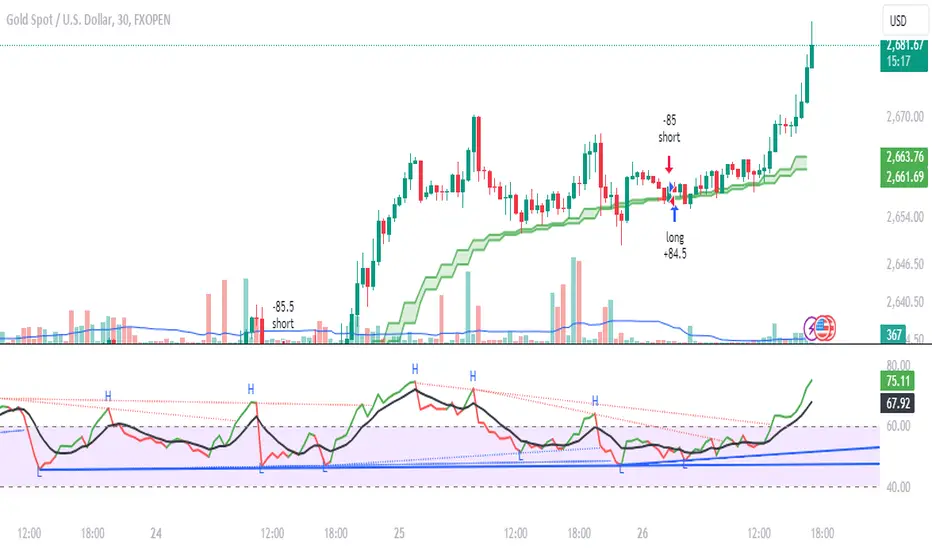
Daksh RSI POINT to ShootHere are the key points and features of the Pine Script provided:
### 1. **Indicator Settings**:
- The indicator is named **"POINT and Shoot"** and is set for non-overlay (`overlay=false`) on the chart.
- `max_bars_back=4000` is defined, indicating the maximum number of bars that the script can reference.
### 2. **Input Parameters**:
- `Src` (Source): The price source, default is `close`.
- `rsilen` (RSI Length): The length for calculating RSI, default is 20.
- `linestylei`: Style for the trend lines (`Solid` or `Dashed`).
- `linewidth`: Width of the plotted lines, between 1 and 4.
- `showbroken`: Option to show broken trend lines.
- `extendlines`: Option to extend trend lines.
- `showpivot`: Show pivot points (highs and lows).
- `showema`: Show a weighted moving average (WMA) line.
- `len`: Length for calculating WMA, default is 9.
### 3. **RSI Calculation**:
- Calculates a custom RSI value using relative moving averages (`ta.rma`), and optionally uses On-Balance Volume (`ta.obv`) if `indi` is set differently.
- Plots RSI values as a green or red line depending on its position relative to the WMA.
### 4. **Pivot Points**:
- Utilizes the `ta.pivothigh` and `ta.pivotlow` functions to detect pivot highs and lows over the defined period.
- Stores up to 10 recent pivot points for highs and lows.
### 5. **Trend Line Drawing**:
- Lines are drawn based on pivot highs and lows.
- Calculates potential trend lines using linear interpolation and validates them by checking if subsequent bars break or respect the trend.
- If the trend is broken, and `showbroken` is enabled, it draws dotted lines to represent these broken trends.
### 6. **Line Management**:
- Initializes multiple lines (`l1` to `l20` and `t1` to `t20`) and uses these lines for drawing uptrend and downtrend lines.
- The maximum number of lines is set to 20 for uptrends and 20 for downtrends, due to a limit on the total number of lines that can be displayed on the chart.
### 7. **Line Style and Color**:
- Defines different colors for uptrend lines (`ulcolor = color.red`) and downtrend lines (`dlcolor = color.blue`).
- Line styles are determined by user input (`linestyle`) and use either solid or dashed patterns.
- Broken lines use a dotted style to indicate invalidated trends.
### 8. **Pivot Point Plotting**:
- Plots labels "H" and "L" for pivot highs and lows, respectively, to visually indicate turning points on the chart.
### 9. **Utility Functions**:
- Uses helper functions to get the values and positions of the last 10 pivot points, such as `getloval`, `getlopos`, `gethival`, and `gethipos`.
- The script uses custom logic for line placement based on whether the pivots are lower lows or higher highs, with lines adjusted dynamically based on price movement.
### 10. **Plotting and Visuals**:
- The main RSI line is plotted using a color gradient based on its position relative to the WMA.
- Horizontal lines (`hline1` and `hline2`) are used for visual reference at RSI levels of 60 and 40.
- Filled regions between these horizontal lines provide visual cues for potential overbought or oversold zones.
These are the main highlights of the script, which focuses on trend detection, visualization of pivot points, and dynamic line plotting based on price action.
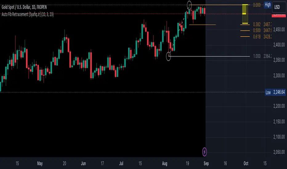
Auto Fib Retracement [Syafiq.Jr]This TradingView script is an advanced indicator titled "Auto Fib Retracement Neo ." It's designed to automatically plot Fibonacci retracement levels on a price chart, aiding in technical analysis for traders. Here's a breakdown of its functionality:
Core Functionality :
The script identifies pivot points (highs and lows) on a chart and draws Fibonacci retracement lines based on these points. The lines are dynamic, updating in real-time as the market progresses.
Customizable Inputs :
Depth: Determines the minimum number of bars considered in the pivot point calculation.
Deviation: Adjusts the sensitivity of the script in identifying new pivots.
Fibonacci Levels: Allows users to select which retracement levels (236, 382, 500, 618, 786, 886) are displayed on the chart.
Visual Settings: Customization options include the colors and styles of pivot points, trend lines, and the retracement meter.
Pivot and Line Calculation:
The script calculates the deviation between the current price and the last pivot point. If the deviation exceeds a certain threshold, it identifies a new pivot and draws a trend line between the previous pivot and the current one.
Visual Aids :
The indicator provides extensive visual aids, including pivot points marked with circles, dashed trend lines connecting pivots, and labels displaying additional information like price and delta rate.
Performance :
Optimized to handle large datasets, the script is configured to process up to 4000 bars and can manage numerous lines and labels efficiently.
Background and Appearance :
The script allows for customization of the chart background color, enhancing visibility based on user preferences.
In essence, this script is a powerful tool for traders who rely on Fibonacci retracement levels to identify potential support and resistance areas, allowing for a more automated and visually guided approach to market analysis.
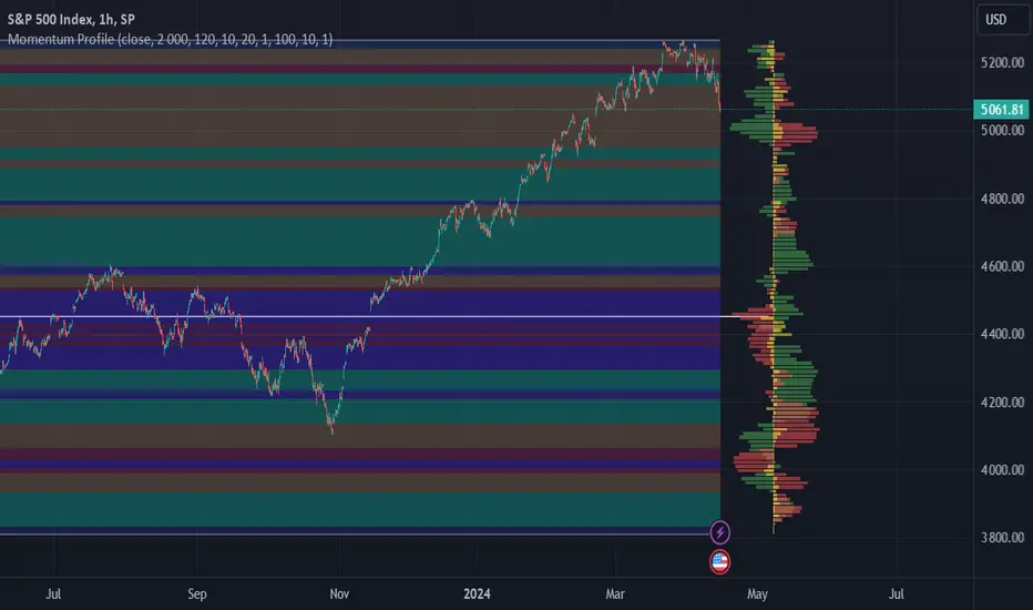
Momentum ProfileProfile market behavior in horizontal zones
Profile Sidebar
Buckets pointing rightward indicate upward security movement in the lookahead window at that level, and buckets pointing leftward indicate downward movement in the lookahead window.
Green profile buckets indicate the security's behavior following an uptrend in the lookbehind window. Conversely, Red profile buckets show security's behavior following a downtrend in the lookbehind window. Yellow profile buckets show behavior following sideways movement.
Buckets length corelates with the amount of movement measured in that direction at that level.
Inputs
Length determines how many bars back are considered for the calculation. On most securities, this can be increased to just above 4000 without issues.
Rows determines the number of buckets that the securities range is divided into.
You can increase or decrease the threshold for which moves are considered sideways with the sideways_filter input: higher means more moves are considered sideways.
The lookbehind input determines the lookbehind window. Specifically, how many bars back are considered when determining whether a data point is considered green (uptrend), red (downtrend), or yellow (no significant trend).
The lookahead input determines how many bars after the current bar are considered when determining the length and direction of each bucket (leftward for downward moves, rightward for upward moves).
Profile_width and Profile_spacing are cosmetic choices.
Intrabar support is not current supported.
Region Highlighting
Regions highlighted green saw an upward move in the lookahead window for both lookbehind downtrends and uptrends. In other words, both red and green profile buckets pointed rightward.
Regions highlighted red saw a downward move in the lookahead window both for lookbehind downtrends and uptrends.
Regions highlighted brown indicate a reversal region: uptrends were followed by downtrends, and vice versa. These regions often indicate a chop range or sometimes support/resistance levels. On the profile, this means that green buckets pointed left, and red buckets pointed right.
Regions highlighted purple indicate that whatever direction the security was moving, it continued that way. On the profile, this means that green buckets pointed right, and red buckets pointed left in that region.
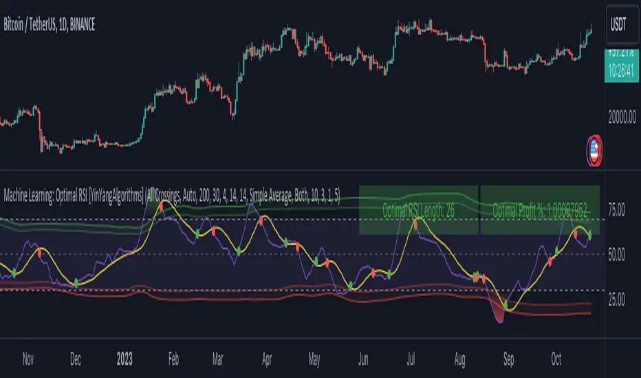
Machine Learning: Optimal RSI [YinYangAlgorithms]This Indicator, will rate multiple different lengths of RSIs to determine which RSI to RSI MA cross produced the highest profit within the lookback span. This ‘Optimal RSI’ is then passed back, and if toggled will then be thrown into a Machine Learning calculation. You have the option to Filter RSI and RSI MA’s within the Machine Learning calculation. What this does is, only other Optimal RSI’s which are in the same bullish or bearish direction (is the RSI above or below the RSI MA) will be added to the calculation.
You can either (by default) use a Simple Average; which is essentially just a Mean of all the Optimal RSI’s with a length of Machine Learning. Or, you can opt to use a k-Nearest Neighbour (KNN) calculation which takes a Fast and Slow Speed. We essentially turn the Optimal RSI into a MA with different lengths and then compare the distance between the two within our KNN Function.
RSI may very well be one of the most used Indicators for identifying crucial Overbought and Oversold locations. Not only that but when it crosses its Moving Average (MA) line it may also indicate good locations to Buy and Sell. Many traders simply use the RSI with the standard length (14), however, does that mean this is the best length?
By using the length of the top performing RSI and then applying some Machine Learning logic to it, we hope to create what may be a more accurate, smooth, optimal, RSI.
Tutorial:
This is a pretty zoomed out Perspective of what the Indicator looks like with its default settings (except with Bollinger Bands and Signals disabled). If you look at the Tables above, you’ll notice, currently the Top Performing RSI Length is 13 with an Optimal Profit % of: 1.00054973. On its default settings, what it does is Scan X amount of RSI Lengths and checks for when the RSI and RSI MA cross each other. It then records the profitability of each cross to identify which length produced the overall highest crossing profitability. Whichever length produces the highest profit is then the RSI length that is used in the plots, until another length takes its place. This may result in what we deem to be the ‘Optimal RSI’ as it is an adaptive RSI which changes based on performance.
In our next example, we changed the ‘Optimal RSI Type’ from ‘All Crossings’ to ‘Extremity Crossings’. If you compare the last two examples to each other, you’ll notice some similarities, but overall they’re quite different. The reason why is, the Optimal RSI is calculated differently. When using ‘All Crossings’ everytime the RSI and RSI MA cross, we evaluate it for profit (short and long). However, with ‘Extremity Crossings’, we only evaluate it when the RSI crosses over the RSI MA and RSI <= 40 or RSI crosses under the RSI MA and RSI >= 60. We conclude the crossing when it crosses back on its opposite of the extremity, and that is how it finds its Optimal RSI.
The way we determine the Optimal RSI is crucial to calculating which length is currently optimal.
In this next example we have zoomed in a bit, and have the full default settings on. Now we have signals (which you can set alerts for), for when the RSI and RSI MA cross (green is bullish and red is bearish). We also have our Optimal RSI Bollinger Bands enabled here too. These bands allow you to see where there may be Support and Resistance within the RSI at levels that aren’t static; such as 30 and 70. The length the RSI Bollinger Bands use is the Optimal RSI Length, allowing it to likewise change in correlation to the Optimal RSI.
In the example above, we’ve zoomed out as far as the Optimal RSI Bollinger Bands go. You’ll notice, the Bollinger Bands may act as Support and Resistance locations within and outside of the RSI Mid zone (30-70). In the next example we will highlight these areas so they may be easier to see.
Circled above, you may see how many times the Optimal RSI faced Support and Resistance locations on the Bollinger Bands. These Bollinger Bands may give a second location for Support and Resistance. The key Support and Resistance may still be the 30/50/70, however the Bollinger Bands allows us to have a more adaptive, moving form of Support and Resistance. This helps to show where it may ‘bounce’ if it surpasses any of the static levels (30/50/70).
Due to the fact that this Indicator may take a long time to execute and it can throw errors for such, we have added a Setting called: Adjust Optimal RSI Lookback and RSI Count. This settings will automatically modify the Optimal RSI Lookback Length and the RSI Count based on the Time Frame you are on and the Bar Indexes that are within. For instance, if we switch to the 1 Hour Time Frame, it will adjust the length from 200->90 and RSI Count from 30->20. If this wasn’t adjusted, the Indicator would Timeout.
You may however, change the Setting ‘Adjust Optimal RSI Lookback and RSI Count’ to ‘Manual’ from ‘Auto’. This will give you control over the ‘Optimal RSI Lookback Length’ and ‘RSI Count’ within the Settings. Please note, it will likely take some “fine tuning” to find working settings without the Indicator timing out, but there are definitely times you can find better settings than our ‘Auto’ will create; especially on higher Time Frames. The Minimum our ‘Auto’ will create is:
Optimal RSI Lookback Length: 90
RSI Count: 20
The Maximum it will create is:
Optimal RSI Lookback Length: 200
RSI Count: 30
If there isn’t much bar index history, for instance, if you’re on the 1 Day and the pair is BTC/USDT you’ll get < 4000 Bar Indexes worth of data. For this reason it is possible to manually increase the settings to say:
Optimal RSI Lookback Length: 500
RSI Count: 50
But, please note, if you make it too high, it may also lead to inaccuracies.
We will conclude our Tutorial here, hopefully this has given you some insight as to how calculating our Optimal RSI and then using it within Machine Learning may create a more adaptive RSI.
Settings:
Optimal RSI:
Show Crossing Signals: Display signals where the RSI and RSI Cross.
Show Tables: Display Information Tables to show information like, Optimal RSI Length, Best Profit, New Optimal RSI Lookback Length and New RSI Count.
Show Bollinger Bands: Show RSI Bollinger Bands. These bands work like the TDI Indicator, except its length changes as it uses the current RSI Optimal Length.
Optimal RSI Type: This is how we calculate our Optimal RSI. Do we use all RSI and RSI MA Crossings or just when it crosses within the Extremities.
Adjust Optimal RSI Lookback and RSI Count: Auto means the script will automatically adjust the Optimal RSI Lookback Length and RSI Count based on the current Time Frame and Bar Index's on chart. This will attempt to stop the script from 'Taking too long to Execute'. Manual means you have full control of the Optimal RSI Lookback Length and RSI Count.
Optimal RSI Lookback Length: How far back are we looking to see which RSI length is optimal? Please note the more bars the lower this needs to be. For instance with BTC/USDT you can use 500 here on 1D but only 200 for 15 Minutes; otherwise it will timeout.
RSI Count: How many lengths are we checking? For instance, if our 'RSI Minimum Length' is 4 and this is 30, the valid RSI lengths we check is 4-34.
RSI Minimum Length: What is the RSI length we start our scans at? We are capped with RSI Count otherwise it will cause the Indicator to timeout, so we don't want to waste any processing power on irrelevant lengths.
RSI MA Length: What length are we using to calculate the optimal RSI cross' and likewise plot our RSI MA with?
Extremity Crossings RSI Backup Length: When there is no Optimal RSI (if using Extremity Crossings), which RSI should we use instead?
Machine Learning:
Use Rational Quadratics: Rationalizing our Close may be beneficial for usage within ML calculations.
Filter RSI and RSI MA: Should we filter the RSI's before usage in ML calculations? Essentially should we only use RSI data that are of the same type as our Optimal RSI? For instance if our Optimal RSI is Bullish (RSI > RSI MA), should we only use ML RSI's that are likewise bullish?
Machine Learning Type: Are we using a Simple ML Average, KNN Mean Average, KNN Exponential Average or None?
KNN Distance Type: We need to check if distance is within the KNN Min/Max distance, which distance checks are we using.
Machine Learning Length: How far back is our Machine Learning going to keep data for.
k-Nearest Neighbour (KNN) Length: How many k-Nearest Neighbours will we account for?
Fast ML Data Length: What is our Fast ML Length? This is used with our Slow Length to create our KNN Distance.
Slow ML Data Length: What is our Slow ML Length? This is used with our Fast Length to create our KNN Distance.
If you have any questions, comments, ideas or concerns please don't hesitate to contact us.
HAPPY TRADING!
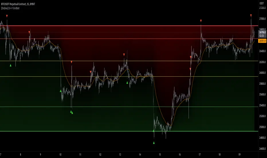
[DisDev] D-I-Y Gridbot🟩 This script is a “do-it-yourself” Grid Bot Simulator, used for visualizing support and resistance levels. Prices are divided into grids, or trade zones, that will trigger signals each time a new zone is entered. During ranging markets, each transaction is followed by a “take profit.” As the market starts to trend, transactions are stacked (compare to DCA ), until the market consolidates. No signals are triggered above the upper gridline or below the lower gridline. Unlike the previous version, all grids may be adjusted in real-time by dragging the gridlines up and down to the desired support and resistance levels.
When adding the indicator to a new chart, you must choose six grid levels by clicking on the desired support or resistance price. You can change all of these levels at any time directly on the chart.
⚡ OVERVIEW ⚡
The D-I-Y Gridbot is an interactive tool designed for visualizing support and resistance levels. As a continuation of the original Gridbot Simulator , which has received significant recognition on TradingView, earning over 4000 boosts and an Editor's Pick status. This tool serves not only as an evolved version of its predecessor, but also as an open-source template for developing future gridbots. It aims to foster discussions and facilitate innovations around grid-trading strategies.
One of the new features of this gridbot is the real-time adjustability of all gridlines. Users can move these lines up and down to set their desired support and resistance levels in response to changing market conditions. Additionally, the D-I-Y Gridbot is compatible with multiple timeframes and can be used on most TradingView charts.
Drag gridlines up or down to desired price level.
Key Features 🔑
All gridlines are adjustable in real-time, directly on the chart
Signals can be filtered by a customizable moving average or by VWAP
Customizable support and resistance levels
Potentially increases profitability in ranging markets
Benefits 💸
Customizable Support and Resistance Levels : The D-I-Y Gridbot allows users to set their preferred support and resistance levels, which can be changed at any time directly on the chart. This provides users with the ability to customize their trading parameters based on their strategy and risk tolerance.
Various Trading Strategies : The D-I-Y Gridbot supports various trading strategies, including Mean Reversion, Ranging Markets, and Dollar-cost averaging (DCA). This allows users to capitalize on price reversals, execute buy and sell orders at predetermined levels, and buy more of an asset as the price falls, respectively.
Multi-Timeframe and Versatility : The D-I-Y Gridbot is compatible with multiple timeframes and can be used on any TradingView chart.
Experimental and Educational : The D-I-Y Gridbot is considered a proof-of-concept tool that is both experimental and educational. This can provide traders with a deeper understanding of grid trading strategies and the ability to experiment with different trading parameters and strategies.
⚙️ CONFIGURATION & SETTINGS ⚙️
Inputs 🔧
Trigger : Candle location to trigger the signal. "Wick" will use either high or low, depending on the signal direction. "Close" will use the close price. “MA” will use the selected moving average or VWAP.
Confirmation : Market direction to confirm the candle trigger. "Reverse" will confirm the signal when the price crosses back over the trigger. "Breakout" will confirm when the price breaks out of the trigger.
Number of Support/Resistance zones : 1 = Only Top Grid is Support/Only Bottom Grid is Resistance. 2 = Top two grids are Resistance/Bottom two grids are Support. 3 = Top three grids are Resistance/Bottom three grids are Support
MA Type : Exponential Moving Average (EMA), Hull Moving Average (HMA), Simple Moving Average (SMA), Triple Exponential Moving Average (TEMA), Volume Weighted Moving Average (VWMA), Volume Weighted Average Price (VWAP)
MA Filter : Use Moving Average as a reversion filter for signals. When enabled, no buys when above MA, no sells when below. Use in conjunction with S/R zones to reduce false signals.
Allow Repeat Signals . When enabled, signals will reset when nearest gridline is triggered. When disabled, only one signal will be triggered per gridline.
Line/Fill colors
Gridlines . Adjusts gridline prices manually.
Left : Trigger = Wick. Confirm = Breakout. Buys are signaled when LOW breaks below gridline. Sells are triggered when HIGH breaks above gridline.
Right : Trigger = Close. Confirm = Breakout. Buys are signaled when the candle CLOSES below the gridline. Sells are triggered when the candle CLOSES above the gridline.
Left : Confirm=Breakout. Signals on breaking through the next gridline.
Right : Confirm=Reverse. Signals only when crossing back from the gridline.
S/R Zones=1. Upper gridline is Resistance / Lower is Support. Middle 4 are neutral.
S/R Zones = 3. Upper three gridlines are Resistance / Lower three are Support
Notes:
If gridlines are dragged out of order on a live chart, they will auto-sort into the correct order.
Price levels may be entered in settings, or adjusted in real-time directly on the chart.
When changing symbols, remember to adjust the gridlines to accommodate the new symbol.
Alerts 🔔
Users can set alerts based on their chosen parameters for triggers, confirmations, number of support/resistance zones, and smoothing type, enabling precise control over alert conditions.
💡 USAGE & STRATEGY 💡
Trading Strategies 📈
Mean Reversion: The script can be used to capitalize on price reversals back to the mean.
Ranging Markets: The script excels in ranging markets, executing buy and sell orders at predetermined levels.
Dollar-cost averaging (DCA): The script can be used to execute DCA orders, buying more of an asset as the price falls, and lowering the average cost per unit.
Timeframes and Symbols ⌚
Multi-Timeframe: The indicator is compatible with multiple timeframes.
Versatile: Can be used on any crypto trading pair on TradingView.
🤖 DETAILS & METHODOLOGY 🤖
Algorithm and Calculation 🛡️
Grids are set and adjusted when loading the indicator on the chart and may be customized anytime afterward by clicking and dragging the gridlines on the chart.
Gridlines are updated, sorted, and stored in a float array.
Signals are calculated based on candle trigger, market direction, and previous price level.
📚 ADDITIONAL RESOURCES 📚
Chart Examples 📊
S/R Zones = 3: Three Support and Three Resistance. Filter = 50-period Triple Exponential Moving Average (TEMA)
S/R Zones = 1: One Support, One Resistance, and Four Neutral Zones. Support Zones: Buys only. Resistance Zones: Sells only. Neutral Zones: Grid-dependent
When MA filter is enabled, Buys are only triggered below Moving Average, and Sells are only triggered above.
Trigger = Wick. Confirmation = Breakout. Buys are signaled when Low breaks above the next grid level. Sells are signaled when High breaks below the next grid level.
🚀 CONCLUSION 🚀
The D-I-Y Gridbot is a proof-of-concept, emphasizing its experimental and educational nature. In future versions, we will aim to incorporate concepts such as auto-adjusting grids and angled grids for trending markets. The script is designed to evolve through user feedback and suggestions, shaping its future iterations.
Credit: This is a continuation of the Gridbot series by xxattaxx-DisDev . Explicit permission was granted by user xxattaxx-disdev to re-use all Gridbot code and all materials without restrictions.
⚠️ DISCLAIMER ⚠️
This indicator is a proof-of-concept and is considered experimental and educational. When gridlines are drawn in hindsight, signals appear to be predictive and valid. Future results may always vary when the trend direction changes. Comments and suggestions are encouraged.
This indicator is provided as a tool for traders and should not be used as the sole basis for making trading decisions. Always conduct your own research and consider your risk tolerance before entering any trades.
Trail Blaze - (Multi Function Trailing Stop Loss) - [mutantdog]Shorter version:
As the title states, this is a 'Trailing Stop' type indicator, albeit one with a whole bunch of additional functionality, making it far more versatile and customisable than a standard trailing stop.
The main set of features includes:
Three independent trailing types each with their own +/- multipliers:
- Standard % change
- ATR (aka Supertrend)
- IQR (inter-quartile range)
These can be used in isolation or summed together. A subsequent pair of direction specific multipliers are also included.
Two separate custom source inputs are available, both feature the standard options alongside a selection of 'weighted inputs' and the option to use another indicator (selected via 'AUX'):
- 'Centre' determines the value about which the trailing sum will be added to define the stop level.
- 'Trigger' determines the value used for crossing of stops, initiating trend changes and triggering alerts.
A selection of optional filters and moving averages are available for both.
Furthermore there are various useful visualisation options available, including the underlying bands that govern the stop levels. Preset alerts for trend reversals are also included.
This is not really an 'out-of-the-box' indicator. Depending upon the market and timeframe some adjustments will be necessary for it to function in a useful manner, these can be as simple or complex as the feature-set allows. Basic settings are easy to dial in however and the default state is intended as a good starting point. Alternatively with some experimentation, a plethora of unique and creative configurations are possible, making this a great tool for tweaking. Below is a more detailed overview followed by a bunch of simple example settings.
------------------------
Lengthy Version :
DESIGN & CONCEPT
Before we start breaking this down, a little background. This started off as an attempt to improve upon the ever-popular Supertrend indicator. Of course there are many excellent user created variants available utilising some interesting methods to overcome the drawbacks of the basic version. To that end, rather than copying the work of others, the direction here shifted towards a hybrid trailing stop loss with a bunch of additional user customisation options. At some point, a completely different project involving IQR got morphed into this one. After sitting through months of sideways chop (where this proved to be of limited use), at the time of publication the market has began to form some near term trend direction and it appears to be performing well in many different timeframes.
And so with that out of the way...
INPUTS
The standard Supertrend (and most other variants) includes a single source input, as default set to 'hl2' (candle mid-range). This is the centre around which the atr bands are added/subtracted to govern the stop levels. This is not however the value which is used to trigger the trend reversal, that is usually hard-coded to 'close'. For this version both source values are adjustable: labelled 'centre' and 'trigger' respectively.
Each has custom input selectors including the usual options, a selection of 'weighted inputs' and the option to use another indicator (selected from the Aux input). The 'weighted inputs' are those introduced in Weight Gain 4000, for more details please refer to that listing. These should be treated as experimental, however may prove useful in certain configurations. In this case 'hl-oc2' can be considered an estimate of the candle median and may be a good alternative to the default 'centre' setting of 'hl2', in contrast 'cc-ohlc4' can tend to favour the extremes in the trend direction so could be useful as a faster 'trigger' than the default 'close'.
To cap them off both come with a selection of moving average filters (SMA, EMA, WMA, RMA, HMA, VWMA and a simple VWEMA - note: not elastic) aswell as median and mid-range. 'Centre' can also be set to the output of 'trigger' post-filter which can be useful if working with fast/slow crosses as the basis.
DYNAMICS
This is the main section, comprised of three separate factors: 'TSL', 'ATR' and 'IQR'. The first two should be fairly obvious, 'TSL' (trailing stop loss) is simply a percentage of the 'centre' value while 'ATR' (average true range) is the standard RMA-based version as used in Supertrend, Volatility Stop etc.
The third factor is less common however: 'IQR' (inter-quartile range). In case you are unfamiliar the principle here is, for a given dataset, the greatest 25% and smallest 25% of samples are removed. The remainder is then treated as a set and the range is calculated by highest - lowest. This is a commonly used method in statistical analysis, by removing the extremes it is less prone to influence by outliers and gives a good representation of the main dispersion around the median. In practise i have found it can be a good alternative to ATR, translating better across multiple time-frames due to it representing a fraction of the total range rather than an average of per-candle range like ATR. Used in combination with the others it can also add a factor more representative of longer-term/higher-timeframe trend. By discarding outliers it also benefits from not being impacted by brief pumps/volatility, instead responding only to more sustained changes in trend, such as rallies and parabolic moves. In order to give an accurate result the IQR is calculated using a dataset of high, low and hlcc4 values for all bars within the lookback length. Once calculated this value is then halved which, strictly speaking, makes it a semi-interquartile range.
All three of these components can be used individually or summed together to create a hybrid dynamics factor. Furthermore each multiplier can be set to both positive and negative values allowing for some interesting and creative possibilities. An optional smoothing filter can be applied to the sum, this is a basic SWMA-4 which is can reduce the impact of sudden changes but does incur a noticeable lag. Finally, a basic limiter condition has been hard-coded here to prevent the sum total from ever going below zero.
Capping off this section is a pair of direction multipliers. These simply take the prior dynamics sum and allow for further multiplication applied only to one side (uptrend/lo-stop and downtrend/hi-stop). To see why this is useful consider that markets often behave differently in each direction, we've all seen prices steadily climb over several weeks and then abruptly dump in the process of a day or two, shorter time frames are no stranger to this either. A lack of downside liquidity, a panicked market, aggressive shorts. All these things contribute to significant differences in downward price action. This function allows for tighter stops in one direction compared to the other to reflect this imbalance.
VISUALISATIONS
With all of these options and possibilities, some visual aids are useful. Beneath the dynamics' section are several visual options including both sources post-filter and the actual 'bands' created by the dynamics. These are what govern the stop levels and seeing them in full can help to better understand what our various configurations actually do. We can even hide the stop levels altogether and just use the bands, making this a kind of expanded Keltner Channel. Here we can also find colour and opacity settings for everything we've discussed.
EXAMPLES
The obvious first example here is the standard %-change trailing stop loss which, from my experience, tends to be the best suited for lower time frames. Filtering should probably minimal here. In both charts here we use the default config for source inputs, the top is a standard bi-directional setup with 1.5% tsl while the bottom uses a 2.5% tsl with the histop multiplier reduced to 0 resulting in an uptrend only stoploss.
Shown here in grey is the standard Supertrend which uses 'hl2' as centre and 'close' as trigger, ATR(10) multiplied by 3. On top we have the default filtered source config with ATR(8) multiplied by 2 which gives a different yet functionally similar result, below is the same source config instead using IQR(12) multiplied by 2. Notice here the more 'stepped' response from IQR following the central rally, holding back for a while before closing in on price and ultimately initiating reversal much sooner. Unlike ATR, the length parameter for IQR is absolute and can more significantly affect its responsiveness.
Next we focus on the visualisation options, on top we have the default source config with ATR(8) multiplied by 2 and IQR(12) multiplied by 1. Here we have activated the switch to show 'bands', from this we can see the actual summed dynamics and how it influences the stop levels. Below that we have an altogether different config utilising the included filters which are now visible. In this example we have created a basic 8/21 EMA cross and set a 1% TSL, notice the brief fakeout in the middle which ordinarily might indicate a buy signal. Here the TSL functions as an additional requirement which in this case is not met and thus no buy signal is given.
Finally we have a couple of more 'experimental' examples. On top we have Lazybear's 'Variable Moving Average' in white which has been assigned via 'aux' as the centre with no additional filtering, the default config for trigger is used here and a basic TSL of 1.5% added. It's a simple example but it shows how this can be applied to other indicators. At the bottom we return to the default source config, combining a TSL of 8% with IQR(24) multiplied by -2. Note here the negative IQR with greater length which causes the stop to close in on price following significant deviations while otherwise remaining fairly wide. Combining positive and negative multiples of each factor can yield mixed results, some more useful than others depending upon suitable market conditions.
Since this has been quite lengthy, i shall leave it there. Suffice to say that there are plenty more ways to use this besides these examples. Please feel free to share any of your own ideas in the comments below. Enjoy.

Weight Gain 4000 - (Adjustable Volume Weighted MA) - [mutantdog]Short Version:
This is a fairly self-contained system based upon a moving average crossover with several unique features. The most significant of these is the adjustable volume weighting system, allowing for transformations between standard and weighted versions of each included MA. With this feature it is possible to apply partial weighting which can help to improve responsiveness without dramatically altering shape. Included types are SMA, EMA, WMA, RMA, hSMA, DEMA and TEMA. Potentially more will be added in future (check updates below).
In addition there are a selection of alternative 'weighted' inputs, a pair of Bollinger-style deviation bands, a separate price tracker and a bunch of alert presets.
This can be used out-of-the-box or tweaked in multiple ways for unusual results. Default settings are a basic 8/21 EMA cross with partial volume weighting. Dev bands apply to MA2 and are based upon the type and the volume weighting. For standard Bollinger bands use SMA with length 20 and try adding a small amount of volume weighting.
A more detailed breakdown of the functionality follows.
Long Version:
ADJUSTABLE VOLUME WEIGHTING
In principle any moving average should have a volume weighted analogue, the standard VWMA is just an SMA with volume weighting for example. Actually, we can consider the SMA to be a special case where volume is a constant 1 per bar (the value is somewhat arbitrary, the important part is that it's constant). Similar principles apply to the 'elastic' EVWMA which is the volume weighted analogue of an RMA. In any case though, where we have standard and weighted variants it is possible to transform one into the other by gradually increasing or decreasing the weighting, which forms the basis of this system. This is not just a simple multiplier however, that would not work due to the relative proportions being the same when set at any non zero value. In order to create a meaningful transformation we need to use an exponent instead, eg: volume^x , where x is a variable determined in this case by the 'volume' parameter. When x=1, the full volume weighting applies and when x=0, the volume will be reduced to a constant 1. Values in between will result in the respective partial weighting, for example 0.5 will give the square root of the volume.
The obvious question here though is why would you want to do this? To answer that really it is best to actually try it. The advantages that volume weighting can bring to a moving average can sometimes come at the cost of unwanted or erratic behaviour. While it can tend towards much closer price tracking which may be desirable, sometimes it needs moderating especially in markets with lower liquidity. Here the adjustability can be useful, in many cases i have found that adding a small amount of volume weighting to a chosen MA can help to improve its responsiveness without overpowering it. Another possible use case would be to have two instances of the same MA with the same length but different weightings, the extent to which these diverge from each other can be a useful indicator of trend strength. Other uses will become apparent with experimentation and can vary from one market to another.
THE INCLUDED MODES
At the time of publication, there are 7 included moving average types with plans to add more in future. For now here is a brief explainer of what's on offer (continuing to use x as shorthand for the volume parameter), starting with the two most common types.
SMA: As mentioned above this is essentially a standard VWMA, calculated here as sma(source*volume^x,length)/sma(volume^x,length). In this case when x=0 then volume=1 and it reduces to a standard SMA.
RMA: Again mentioned above, this is an EVWMA (where E stands for elastic) with constant weighting. Without going into detail, this method takes the 1/length factor of an RMA and replaces it with volume^x/sum(volume^x,length). In this case again we can see that when x=0 then volume=1 and the original 1/length factor is restored.
EMA: This follows the same principle as the RMA where the standard 2/(length+1) factor is replaced with (2*volume^x)/(sum(volume^x,length)+volume^x). As with an RMA, when x=0 then volume=1 and this reduces back to the standard 2/(length+1).
DEMA: Just a standard Double EMA using the above.
TEMA: Likewise, a standard Triple EMA using the above.
hSMA: This is the same as the SMA except it uses harmonic mean calculations instead of arithmetic. In most cases the differences are negligible however they can become more pronounced when volume weighting is introduced. Furthermore, an argument can be made that harmonic mean calculations are better suited to downtrends or bear markets, in principle at least.
WMA: Probably the most contentious one included. Follows the same basic calculations as for the SMA except uses a WMA instead. Honestly, it makes little sense to combine both linear and volume weighting in this manner, included only for completeness and because it can easily be done. It may be the case that a superior composite could be created with some more complex calculations, in which case i may add that later. For now though this will do.
An additional 'volume filter' option is included, which applies a basic filter to the volume prior to calculation. For types based around the SMA/VWMA system, the volume filter is a WMA-4, for types based around the RMA/EVWMA system the filter is a RMA-2.
As and when i add more they will be listed in the updates at the bottom.
WEIGHTED INPUTS
The ohlc method of source calculations is really a leftover from a time when data was far more limited. Nevertheless it is still the method used in charting and for the most part is sufficient. Often the only important value is 'close' although sometimes 'high' and 'low' can be relevant also. Since we are volume weighting however, it can be useful to incorporate as much information as possible. To that end either 'hlc3' or 'hlcc4' tend to be the best of the defaults (in the case of 24/7 charting like crypto or intraday trading, 'ohlc4' should be avoided as it is effectively the same as a lagging version of 'hlcc4'). There are many other (infinitely many, in fact) possible combinations that can be created, i have included a few here.
The premise is fairly straightforward, by subtracting one value from another, the remaining difference can act as a kind of weight. In a simple case consider 'hl2' as simply the midrange ((high+low)/2), instead of this using 'high+low-open' would give more weight to the value furthest from the open, providing a good estimate of the median. An even better estimate can be achieved by combining that with 'high+low-close' to give the included result 'hl-oc2'. Similarly, 'hlc3' can be considered the basic mean of the three significant values, an included weighted version 'hlc2-o2' combines a sum with subtraction of open to give an estimated mean that may be more accurate. Finally we can apply a similar principle to the close, by subtracting the other values, this one potentially gets more complex so the included 'cc-ohlc4' is really the simplest. The result here is an overbias of the close in relation to the open and the midrange, while in most cases not as useful it can provide an estimate for the next bar assuming that the trend continues.
Of the three i've included, hlc2-o2 is in my opinion the most useful especially in this context, although it is perhaps best considered to be experimental in nature. For that reason, i've kept 'hlcc4' as the default for both MAs.
Additionally included is an 'aux input' which is the standard TV source menu and, where possible, can be set as outputs of other indicators.
THE SYSTEM
This one is fairly obvious and straightforward. It's just a moving average crossover with additional deviation (bollinger) bands. Not a lot to explain here as it should be apparent how it works.
Of the two, MA1 is considered to be the fast and MA2 is considered to be the slow. Both can be set with independent inputs, types and weighting. When MA1 is above, the colour of both is green and when it's below the colour of both is red. An additional gradient based fill is there and can be adjusted along with everything else in the visuals section at the bottom. Default alerts are available for crossover/crossunder conditions along with optional marker plots.
MA2 has the option for deviation bands, these are calculated based upon the MA type used and volume weighted according to the main parameter. In the case of a unweighted SMA being used they will be standard Bollinger bands.
An additional 'source direct' price tracker is included which can be used as the basis for an alert system for price crossings of bands or MAs, while taking advantage of the available weighted inputs. This is displayed as a stepped line on the chart so is also a good way to visualise the differences between input types.
That just about covers it then. The likelihood is that you've used some sort of moving average cross system before and are probably still using one or more. If so, then perhaps the additional functionality here will be of benefit.
Thanks for looking, I welcome any feedack
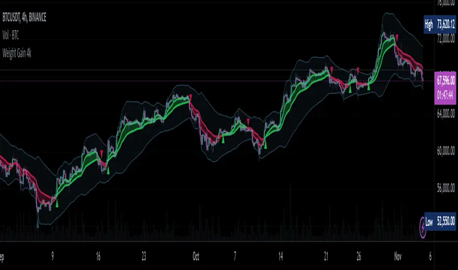
Pinescript - Common String Functions Library by RRBCommon String Functions Library by RagingRocketBull 2021
Version 1.0
Pinescript now has strong support for arrays with many powerful functions, but still lacks built-in string functions. Luckily you can easily process and manipulate strings using arrays.
This script provides a library of common string functions for everyday use, such as: indexOf, substr, replace, ascii_code, str_to_int etc. There are 100+ unique functions (130 including all implementations)
It should serve as building blocks to speed up the development of your custom scripts. You should also be able to learn how Pinescript arrays works and how you can process strings.
Similar libraries for Array and Statistical Functions are in the works. You can find the full list of functions below.
Features:
- 100+ unique string functions (130 including all implementations) in categories: lookup, testing, conversion, modification, extraction, type conversion, date and time, console output
- Live Output for all/selected functions based on User Input. Test any function before using in script.
- Live Unit Test Output for several functions based on pre-defined inputs.
- Output filters: show unique functions/all implementations, grouping
- Console customization options: set custom text size, color, page length
- Support for Pages - auto splits output into pages with fixed length, use pages in your scripts
- Several easy to use console output functions to speed up debugging/output.
WARNING:
- Compilation Time: 1 min
Notes:
- uses Pinescript v3 Compatibility Framework
- this script is packed to the max and sets a new record in testing of Pinescript's limits: 500 local scopes, 4000+ lines, 180kb+ source size. It's not possible to add more ifs/fors/functions without reducing functionality
- to fit the max limit of local scopes = 500 all ifs were replaced with ?: where possible, the number of function calls was reduced, some calls replaced with inline function code
- ifs are faster (especially when lots of them are used in a for cycle), more readable, but ifs/fors/functions increase local scopes (+1) and compiled file size, have max nesting limit = 10.
- ?: are slower (especially in for cycles), hard to read when nested, don't affect local scopes, reduce compiled file size, can't contain plots, for statements (break/continue) and sets of statements
- for most array functions to work (except push), an array must be defined with at least 1 pre-existing dummy element 0.
- if you see "String too long" error - enable Show Pages, reduce Max Chars Per Page < Max String Length limit = 4096.
- if you see "Loop too long" error - hide/unhide or reattach the script
- some functions have several implementations that can be faster/slower, use internal code/ext functions
- 1 is manual string processing using for cycles (array.get) and ext functions - provided in case you want to implement your own logic, may sometimes be slower
- 2 is a 2nd alternate implementation mostly done using built-in functions (array.indexof, array.slice, array.insert, array.remove, str.replace_all),
attempts to minimize local scopes and dependency on ext functions, should generally be faster
- 3 is a 3rd alternate (array.includes, array.fill) or a more advanced implementation (datetime3_str) with lots of params, giving you the most control over output
- most functions have dependencies, such as const names, global arrays, inputs, other functions.
P.S. Strings of Time may be closed unto themselves or have loose ends; they can vibrate, stretch, join or split.
Function Groups:
1. Char Functions
- repeat(str, num)
- ascii_char(code)
- ascii_code(char)
- is_digit(char)
- is_letter(char)
- digit_to_int(char)
- is_space_char(char)
2. Char Test and Lookup Functions
- char_at(str, pos)
- char_code_at(str, pos)
- indexOf_char(str, char)
- lastIndexOf_char(str, char)
- nth_indexOf_char(str, char, num)
- includes_char(str, char)
3. String Lookup Functions
- indexOf(str, target)
- lastIndexOf(str, target)
- nth_indexOf(str, target, num)
- indexesOf(str, target)
- numIndexesOf(str, target)
4. String Conversion Functions
- lowercase(str)
- uppercase(str)
5. String Modification and Extraction Functions
- split(str, separator)
- insert(str, pos, new_str)
- remove(str, pos, length)
- insert_char(str, pos, char)
- remove_char(str, pos)
- reverse(str)
- fill_char(str, char, start_pos, end_pos)
- replace(str, target, new_str)
- replace_first(str, target, new_str)
- replace_last(str, target, new_str)
- replace_nth(str, target, new_str, num)
- replace_left(str, new_str)
- replace_right(str, new_str)
- replace_middle(str, pos, new_str)
- left(str, num)
- right(str, num)
- first_char(str)
- last_char(str)
- truncate(str, max_len)
- truncate_middle2(str, trunc_str, pos, max_len)
- truncate_from2(str, trunc_str, pos, max_len, side)
- concat(str1, str2, trunc_str, max_len, mode)
- concat_from(str1, str2, trunc_str, max_len, side, mode)
- trim(str)
- substr(str, pos, length)
- substring(str, start_pos, end_pos)
- strip(str, mask, target, is_allowed)
- extract_groups(str)
- extract_numbers(str, d1, d2, mode)
- str_to_float(str, d1, d2)
- str_to_int(str)
- extract_ranges(str, d1, d2, d3, type)
6. String Test Functions
- includes(str, target)
- starts_with(str, target)
- ends_with(str, target)
- str_compare(str1, str2)
7. Type Conversion Functions
- tf_check2(tf)
- tf_to_mins()
- convert_tf(tf)
- period_to_mins(tf)
- convert_tf2(tf)
- convert_tf3(tf)
- bool_to_str(flag)
- get_src(src_str)
- get_size(size_str)
- get_style(style)
- get_bool(bool_str)
- get_int(str)
- get_float(str, d1, d2)
- get_color(str, def_color)
- color_tr2(col_str, transp)
- get_month(str)
- month_name(num, format)
- weekday_name(num, format)
- dayofweek_name(t)
8. Date and Time Functions
- date_str(t, d)
- time_str(t, d)
- datetime_str(t, d1, d2)
- date2_str(t, d, type)
- time2_str(t, d, type)
- datetime2_str(t, d1, d2, format1, format2)
- date3_str(t, template)
- time3_str(t, template)
- datetime3_str(t, template)
9. Console Output & Helper Functions
- echo1(con, str)
- echo2(x, y, con, str)
- echo3(v_shift, con, str, msg_color, text_size)
- echo4(x, y, con, str, msg_style, msg_color, text_size, text_align, msg_xloc)
- echo5(x, y, con, str, msg_style, msg_color, text_size, text_align, msg_xloc)
- echo6(x, y, con, str)
- echo7(v_shift, con, str, msg_color, text_size)
- echo8(x, y, con, str, msg_style, msg_color, text_size, text_align, msg_xloc)
- echo9(x, y, con, str, msg_style, msg_color, text_size, text_align, msg_xloc)
- new_page(str, line_str, trunc_str, header_str, footer_str, length, page_count, page, mode)

Filter Amplitude Response Estimator - A Simple CalculationIn digital signal processing knowing how a system interact with the frequency content of an input signal is extremely important, the mathematical tool that give you this information is called "frequency response". The frequency response regroup two elements, the amplitude response, and the phase response. The amplitude response tells you how the system modify the amplitude of the frequency components in the input signal, the phase response tells you how the system modify the phase of the frequency components in the signal, each being a function of the frequency.
The today proposed tool aim to give a low resolution representation of the amplitude response of any filter.
What Is The Amplitude Response Of A Filter ?
Remember that filters allow to interact with the frequency content of a signal by amplifying, attenuating and/or removing certain frequency components in the input signal, the amplitude (also called magnitude) response of a filter let you know exactly how your filter change the amplitude of the frequency components in the input signal, another way to see the amplitude response is as a tool that tell you what is the peak amplitude of a filter using a sinusoid of a certain frequency as input signal.
For example if the amplitude response of a filter give you a value of 0.9 at frequency 0.5, it means that the filter peak amplitude using a sinusoid of frequency 0.5 is equal to 0.9.
There are several ways to calculate the frequency response of a filter, when our filter is a FIR filter (the filter impulse response is finite), the frequency response of the filter is the absolute value of the discrete Fourier transform (DFT) of the filter impulse response.
If you are curious about this process, know that the DFT of a N samples signal return N values, so if our FIR filter coefficients are composed of only 5 values we would get a frequency response of 5 values...which would not be useful, this is why we "pad" our coefficients with zeros, that is we add zeros to the start and end of our series of coefficients, this process is called "zero-padding", so if our series of coefficients is: (1,2,3,4,5), applying zero padding would give (0,0...1,2,3,4,5,...0,0) while keeping a certain symmetry. This is related to the concept of resolution, a low resolution amplitude response would be composed of a low number of values and would not be useful, this is why we use zero-padding to add more values thus increasing the resolution.
Making a Fourier transform in Pinescript is not doable, as you need the complex number i for computing a DFT, but thats not even the only problem, a DFT would not be that useful anyway (as the processes to make it useful in a trading context would be way too complex) . So how can we calculate a filter amplitude response without using a DFT ? The simple answer is by taking the peak amplitude of a filter using a sinusoid of a certain frequency as input, this is what the proposed tool do.
Using The Tool
The proposed tool give you a 50 point amplitude response from frequency 0.005 to 0.25 by default. the setting "Range Divisor" allow you to see the amplitude response by using a different range of frequency, for example if the range divisor is equal to 2 the filter amplitude response will be evaluated from frequency 0.0025 to 0.125.
In the script, filt hold the filter you want to see the frequency response, by default a simple moving average.
The position of the frequency response is defined by the "Show Amplitude Response At Bar Number" setting, if you want the frequency response to start at bar number 5000 then enter 5000, by default 10000. If you are not a premium set the number at 4000 and it should work.
amplitude response of a simple moving average of period 14, res = 2.
By default the amplitude response use an amplitude scale, a value of 1 represent an unchanged amplitude. You can use Dbfs (decibel full scale) instead by checking the "To Decibels (Full Scale)" setting.
Dbfs amplitude response, a value of 0 represent an unchanged amplitude.
Some Amplitude Responses
In order to prove the accuracy of the proposed tool we can compare the amplitude response given by the proposed tool with the mathematical function of the amplitude response of a simple moving average, that is:
abs(sin(pi*f*length)/(length*sin(pi*f)))
In cyan the amplitude response given by the proposed tool and in blue the above function. Below are the amplitude responses of some moving averages with period 14.
Amplitude response of an EMA, the EMA is a IIR filter, therefore the amplitude response can't be made by taking the DFT of the impulse response (as this ones has infinite length), however our tool can give its frequency response.
Amplitude response of the Hull MA, as you can see some frequencies are amplified, this is common with low-lag filters.
Gaussian moving average (ALMA), with offset = 0.5 and sigma = 6.
Simple moving average high-pass filter amplitude response
Center of gravity bandpass filter amplitude response
Center of gravity bandreject filter.
IMPORTANT!: The amplitude response of adaptive moving averages is not stationary and might change over time.
Conclusion
A tool giving the amplitude response of any filter has been presented, of course this method is not efficient at all and has a low resolution of 50 points (the common resolution is of 512 points) and is difficult to work with, but has the merit to work on Tradingview and can give the frequency response of IIR filters, if you really need to see the frequency response of a filter then i recommend you to use the function freqz from the scipy package.
I still hope you will enjoy using this tool to have a look at the amplitude responses of your favorite moving averages.
I'am aware of the current situation, however i'am somehow feeling left out from the pinescript community, let me know via PM if i have done something to you and i'll do my best to fix any problems i might have caused (or i might be being parano xD)

STDEV 20MA Difference Standard Deviation and 20 Moving Avergae Difference.
This could help some Buy & Sell with Difference between STDEV and 20 MA.
Difference will show us something.
+- 4000 : 1D Buy / Sell Zone
+- 2500 : 6H Buy / Sell Zone
+- 800 : 1H Buy / Sell Zone
Check some point !
Reset Every (Price)Someone requested a high/low price indicator that would reset the "remembered" prices daily. I started out doing just that, and then decided to make it much more configurable.
Choose the units (minutes, hours, days, weeks, months) and the number of those units, and this will reset the highest/lowest value remembered to the current values on your chosen time interval.
This should work with any time interval you desire, within reason...asking for resets every 4000 hours on a monthly chart will probably not work.
GE, monthly, every 7 months:
Ford, weekly, every 18 months:
Dow Jones Industrial Average, weekly, every 90 days:
LTCBTC, daily, every 10 days:
ETHUSD, 30 minutes, every 10 days:
BTCUSD, 1 minute, every 10 hours:
EURUSD, 1 minute, every 50 minutes:
Also, I am about to publish another version of this with just one source input that can be applied to any indicator...stay tuned!

Fibonacci ClustersI was reading about Fibonacci Clusters on investopedia (www.investopedia.com) and couldn't find a script for it on tradingveiw. Apparently some people use it successfully but I found it a little chaotic. This script will mark the retracements in a window's length, and you can set this for six windows. This script isn't very pretty because it doesn't seem obviously useful and pinescript has far too many deficiencies to fully flesh this idea out. I was able to make more sense out of larger windowing times (500-4000 periods), than shorter ones (25-333). Try it out, see what it shows you. Happy trading
