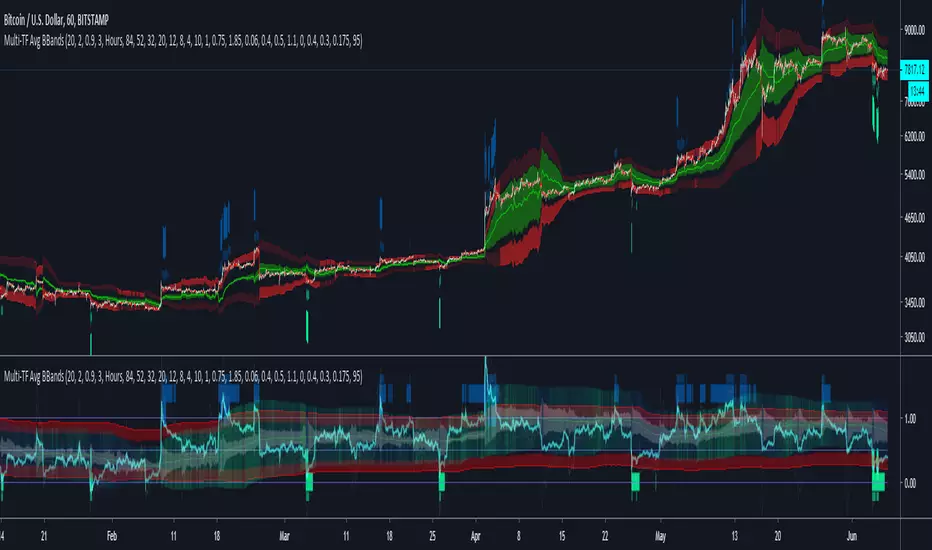
Multi-TF Avg BBandsMULTI-TF AVERAGE BBANDS - with signals (BETA)
Overall, it shows where the price has support and resistance, when it's breaking through, and when its relatively low/high based on the magic of standard deviation.
created by gamazama. send me a shout if u find this useful, or if you create something cool with it.
%BB: The price's position in the boilinger band is converted to a range from 0-1. The midpoint is at 0.5
Description of parameters
"BB:Window Length" is the standard BB size of 20 candles.
The indicator plots up to 7 different %BB's on different timescales
They are calculated independently of the timescale you are viewing eg 12h, 3d, 30m will be the same output
You can enter 7 timescales, eg. if you want to plot a range of bbands of the 12h up to 3d graphs, enter values between 0.5 and 3 (days) - you can also select 0 to disable and use less timescales, or select hours or minutes
Take note if you eg. double the main multiplier to 40, it is the same as doubling all your timescales
You can turn the transparency of the 7 x %BB's to 100 to hide them, their average is plotted as a thick cyan line
"Variance" is a measure of how much the 7 BB's agree, and changes colour based on the thresholds used for the strategy
---- TO START FROM SCRATCH ----
- set all except one to ZERO (0), set to 0, and everything after to 0.
Turn ON and right click -> move the indicator to a new pane - this will show you the internal workings of the indicator.
Then there is a few standard settings
"Source Smoothing Amount" applies a basic small sma on the price.
It should be turned down when viewing candles with less information, like 1D or more.
Standard BBands use an SMA, there one uses a blend between VWMA or SMA
Volume Weight settings, the same as SMA at 0, and the same as VWMA at 1
BB^2 is a bband drawn around the average %BB. Adjust the to change its window length
The BB^2 changes color when price moves up or down
Now its time to look at the parameters which affect the buy/sell signals
turn on "show signal range" - you see some red lines
buy and sell each have 4 settings
min/max variance will affect the brigtness of the signal range
range adjust will move the range up/down
mix BB^2 blends between a straight line (0) and BB^2's top or bottom (1)
a threshold of "variance" and "h/l points" is available to generate weaker signals.
these thresholds can be increased to show more weak signals
ONCE YOU ARE HAPPY WITH THE SIGNALS being generated, you can turn OFF , and move it back to the price pane
the indicator then draws a bband around the price to maps some info into the chart:
fills a colour between 0.5 & the mid BB^2 and converts relative to the price chart
draws a line in the middle of the midband.
controls how much these lines diverge from the price - adjust it to reduce noise
converts the signal range (red lines) to be relative to the price chart
if you like, you can adjust the sell & buy signals in the tab from and to and to match the picture. It messes with auto-scaling when moving back to though
enjoy, I hope that is easy enough to understand, still trying to make this more user-friendly.
If you want to send me some token of appreciation - btc: 33c2oiCW8Fnsy41Y8z2jAPzY8trnqr5cFu
I promise it will put a fat smile on my face
在腳本中搜尋"如何用wind搜索股票的发行价和份数"
Coding ema in pinescriptWhat is EMA ?
Ema is known as exponential moving average, it comes from the class of weighted moving average. It gives more weightage to the recent price changes, thus making it much more relevant to the current market analysis. Also it provides a dynamic way of calculating support and resistances in a trend following setup.
The most common way to mint profit out from the market is to use trend following setups which can be easily achieved by using a group of EMA’s
So how’s this EMA calculated ?
Before understanding the calculation of EMA let’s look into a much wider topic:
“The Law of Averages”
It states : If you do something often enough a ratio will appear, simply put, any time series data, tend to deviate from its average.
EMA provides a way to statistically calculate the exponential moving average for a provided time series data giving much more emphasis on the most recent data in the series.
So in the 17th century, when the people were playing with numbers in their free time, they came up with a statistical strategy to envelop any time series data to detect the direction of the data flow , they called it exponential moving average.
Later in 1940’s with the increase in signal processing requirements in the field of electronic devices scientists started using Exponential moving average onto the electronic signal followers, just to classify the signals as above or below a moving/dynamic threshold.
So EMA is a smoothed time-series data.
The simplest form of EMA Smoothing can be given by the formula:
S(t) = alpha * X(t) + (1 - alpha) * X(t - 1).
The value of alpha must lie between 0 and 1
Where
alpha , is the smoothing factor
X(t) , is the current observation data point
X(t - 1), is the past observational data point.
t , is the current time
Generally,
In current day trading setups for EMA the alpha is calculated by
alpha = 2 / (time period window + 1)
Things to note here is that the alpha calculated above is the most generally used factor calculation method for EMA ,
You can tweak the alpha function above until it gives value between 0 and 1 for example alpha can also be written as
alpha = ln ( current price / past price )
Note it’s just a weighing scheme,
But for Our Case of EMA
We will be using
alpha = 2 / (time period window + 1)
Please refer to the script code below
Support and Resistance linesThis indicator allows you to set 5 SR lines for 8 currency pairs. The SR line variables need to be set in the pine script.
It is easy to add more currency pairs or change the number of SR lines.
The indicator works in the following time frames: 1D, 12H, 8H, 6H, 4H
In the active time frame green and red vertical lines indiate a potential reversal.
Higher time frame occurrences are indicated by e.g. 8H, 12H labels above or below the price line.
So, e.g. in the 12H window you can see D labels. And in the 8H window you can see 12H and D labels.
The indicator recognizes 4 long and 4 short patterns. These patterns are very simple. See the section "Conditions for PriceAction patterns" in the pine script.
If you desire please go ahead and change the patterns or add new ones. This is the most difficult part. If you come up with good ones please post them here.

Mathematical Derivatives of PriceThis indicator is meant to show the Velocity (1st order derivative), Acceleration (2nd order derivative), Jerk (3rd order derivative), Snap (4th order derivative), Crackle (5th order derivative), & Pop (6th order derivative) of price. The values at the top of the indicator window are in this order from left to right. I don't particularly know how this would be used in a trading strategy, but if you're ever curious about how quickly price is moving and how much it is accelerating, then you could use this tool.
*If you only care about velocity and acceleration, and don't like how squished the window is because of the long decimal numbers then edit the "precision" value in the first line of the script to a smaller number of your choosing.*

Chiki-Poki BFXLS Longs Shorts Abs Normalized Volume Pro by RRBChiki-Poki BFXLS Longs vs Shorts Absolute Normalized Volume Value Pro by RagingRocketBull 2018
Version 1.0
This indicator displays Longs vs Shorts in a side by side graph, shows volume's absolute price value and normalized volume of Longs/Shorts for the current asset. This allows for more accurate L/S comparisons (like a log scale for volume) since volume on spot exchanges (Bitstamp, Bitfinex, Coinbase etc) is measured in coins traded, not USD traded. Similarly, L/S is usually the amount of coins in open L/S positions, not their total USD value. On Bitmex and other futures exchanges volume is measured in USD traded, so you don't need to apply the Volume Absolute Price Value checkbox to compare L/S. You should always check first whether your source is measured in coins or USD.
Chiki-Poki BFXLS primarily uses *SHORTS/LONGS feeds from Bitfinex for the current crypto asset, but you can specify custom L/S source tickers instead.
This 2-in-1 works both in the Main Chart and in the indicator pane below. You can switch between Main/Sub Window panes using RMB on the indicator's name and selecting Move To/Pane Above/Below.
This indicator doesn't use volume of the current asset. It uses L/S ticker's OHLC as a source for SHORTS/LONGS volumes instead. Essentially L/S => L/S Volume == L/S
Features:
- Display Longs vs Shorts side by side graph for the current crypto asset, i.e. for BTCUSD - BTCUSDLONGS/BTCUSDSHORTS, for ETHUSD - ETHUSDLONGS/ETHUSDSHORTS etc.
- Use custom OHLC ticker sources for Longs/Shorts from different exchanges/crypto assets with/without exchange prefix.
- Plot Longs/Shorts as lines or candles
- Show/Hide L/S, Diff, MAs, ATH/ATL
- Use Longs/Shorts Volume Absolute Price Value (Price * L/S Volume) instead of Coins Traded in open L/S positions to compare total L/S value/capitalization
- Normalize L/S Volume using Price / Price MA / L/S Volume MA
- Supports any existing type of MA: SMA, EMA, WMA, HMA etc
- Volume Absolute Price Value / Normalize also works on candles
- Oscillator mode with negative axis (works in both Main Chart/Subwindow panes).
- Highlight L/S Volume spikes above L/S MAs in both lines/oscillator.
- Change L/S MA color based on a number of last rising/falling L/S bars, colorize candles
- Display L/S volume as 1000s, mlns, or blns using alpha multiplier
1. based on BFXLS Longs vs Shorts and Compare Style, uses plot*, security and custom hma functions
2. swma has a fixed length = 4, alma and linreg have additional offset and smoothing params
Notes:
- Make sure that Left Price Scale shows up with Auto Fit Data enabled. You can reattach indicator to a different scale in Style.
- It is not recommended to switch modes multiple times due to TradingView's scale reattachment bugs. You should switch between Main Chart and Sub Window only once.
- When the USD price of an asset is lower you can trade more coins but capitalization value won't be as significant as when there are less coins for a higher price. Same goes for Shorts/Longs.
Current ATH in shorts doesn't trigger a squeeze because its total value is now far less than before and we are in a bear market where it's normal to have a higher number of shorts.
- You should always subtract Hedged L/S from L/S because hedged positions are temporary - used to preserve the value of the main position in the opposite direction and should be disregarded as such.
- Low margin rates increase the probability of a move in an underlying direction because it is cheaper. High margin rates => the market is anticipating a move in this direction, thus a more expensive rate. Sudden 5-10x rate raises imply a possible reversal soon. high - 0.1%, avg - 0.01-0.02%, low - 0.001-0.005%
You can also check out:
- BFXLS Longs/Shorts on BFXData
- Bitfinex L/S margin rates and Hedged L/S on datamish
- Bitmex L/S on Coinfarm.online
Kringold2[WOZDUX] gold equivalentThe indicator is a tool for global analysis. The default is the price of gold. The price of the instrument from the main window is divided by the price of gold. The result is the price of the instrument in units of gold. The screen uses the Dow Jones index as an example. In the indicator window, the price of the index in units of gold or the so-called gold Dow Jones. The use of the gold equivalent makes it possible to see more truthful trends. The Indicator has the ability to change gold to any other equivalent. It is enough to change the name of the exchange and the name of the instrument in the options tool and exchange. In addition, in the settings, the second box on top allows you to view the graph in a linear or logarithmic scale. The first box at the top switches the line chart or the CCI =WT indicator to this chart.
-------------------------------------------
Индикатор это инструмент для глобального анализа. По умолчанию используется цена золота. Цена инструмента из основного окна делится на цену золота. В результате получается цена инструмента в единицах золота. На экране для примера используется индекс Доу джонса. В окне индикатора цена индекса в единицах золота или так называемый золотой Доу Джонс. Использование золотого эквивалента дает возможность видеть более правдивые тенденции движения. В Индикаторе есть возможность поменять золото на любой другой эквивалент. Достаточно в опциях инструмент и биржа изменить название биржи и название инструмента. Кроме того, в настройках, второй бокс сверху дает возможность смотреть график в линейном или логарифмическом масштабе. Первый бокс сверу переключает линейный график или индикатор CCI =WT к данному графику.

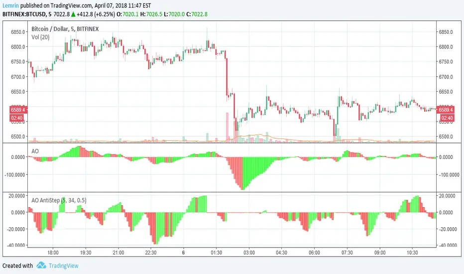
Awesome Oscillator with AntiStep CorrectionHere is the well-known Awesome Oscillator (AO), which I use to present the real purpose of this post: a function that provides step correction for simple moving averages (SMAs).
We all know that any indicator based on moving averages lags real-time movement. Normally this is fine, but just after large ("step") changes in level, the pre-step values that are still within the SMA window cause the result to falsely reflect continued movement, even when real-time values remain flat.
To counter this, when a step change of a configurable size is detected, I temporarily shrink the SMA window size to include only those values occurring since the step change, and then allow the size to increase to normal length as we move away from the step change. This is accomplished within the antistep_sma() function.
Note that this will cause SMAs of different lengths (e.g. those used in the AO) to be temporarily equal, until the shorter of the two reaches its normal size and begins to leave the longer one behind again. You can see this above, where the AO, which is the difference of two SMAs, goes to 0 immediately after a sufficiently large step change--configured to 0.5% in this case.
Hershey's Portfolio WatchThanks to user rwestbury for the idea!
Watch the profit in dollars of your portfolio in REAL TIME, love it!
Put this in a window that doesn't change often, for it takes long to initially load.
I use it in my window where I monitor the US index SPY.
Edit and add as many symbols as you want below, you should be able to figure it out.
Just add symbol, number of shares and price.
I'll improve on this later, like trim the code down with function calls, etc.
Good trading!
Brian Hershey
I_Heikin Ashi CandleWhen apply a strategy to Heikin Ashi Candle chart (HA candle), the strategy will use the open/close/high/low values of the Heikin Ashi candle to calculate the Profit and Loss, hence also affecting the Percent Profitable, Profit Factor, etc., often resulting a unrealistic high Percent Profitable and Profit Factor, which is misleading. But if you want to use the HA candle's values to calculate your indicator / strategy, but pass the normal candle's open/close/high/low values to the strategy to calculate the Profit / Loss, you can do this:
1) set up the main chart to be a normal candle chart
2) use this indicator script to plot a secondary window with indicator looks exactly like a HA-chart
3) to use the HA-candle's open/close/high/low value to calculate whatever indicator you want (you may need to create a separate script if you want to plot this indicator in a separate indicator window)
[RS]Temporal Median Price V1EXPERIMENTAL: previous custom time window median price and current time window open price in a neat package :p
(JeanLouisHardy) added option for bar count system, also added a donchian average.
[RS]Temporal Median Price V0EXPERIMENTAL: previous custom time window median price and current time window open price in a neat package :p
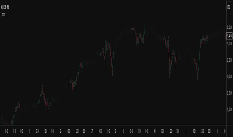
X FocusDesigned to help traders reduce distractions by de-emphasizing specific time ranges on the chart. Instead of highlighting high-activity zones, this tool intentionally applies a muted overlay to selected sessions, allowing traders to concentrate on price action that occurs outside those designated ranges.
Core Purpose
The primary goal of this indicator is to combat the “noise” that often arises during certain periods, such as overnight sessions or pre-market trading. By visually softening those areas, traders can focus on the more relevant trading windows WITHOUT losing any time-based context. Unlike traditional tools that remove data entirely, X Focus preserves all candlestick and price information—ensuring that key levels, gaps, or reference values are still visible.
Key Features
Custom Session Filtering
Users can define up to three time ranges depending on preference. This flexibility allows for tailoring the indicator to different market strategies.
De-Emphasis by Design
Instead of masking or deleting data, the indicator overlays a semi-transparent shading box over the chosen sessions. This ensures traders remain aware of the data while maintaining visual focus on the price action outside of the selected time blocks.
Dual Utility – Highlight or Suppress
While built on the principle of minimizing distractions, the same framework can also be used in reverse to highlight specific areas of interest. This versatility makes it suitable for both noise-reduction and spotlighting critical ranges.
Dark Mode / Light Mode
Adjustable color schemes allow seamless integration into any chart setup, whether the user prefers dark or light backgrounds.
Non-Intrusive Visualization
The shading effect is applied without altering price bars, indicators, or other overlays. This ensures compatibility with existing technical tools and strategies.
Use Case
Traders who find themselves reacting too strongly to inconsequential movements during certain times (such as after-hours or low-volume sessions) can benefit from the X Focus indicator. It helps maintain clarity and discipline by visually guiding attention toward the periods that matter most—without erasing or ignoring potentially useful price references.
Bardhi's ICT Killzone & PivotsThis indicator is a complete ICT-style session and liquidity toolkit designed for precision trading. It automatically marks the most important trading windows (“Killzones”) and provides powerful tools for tracking price action around them.
Key Features:
Killzones: Automatically plots Asia, London, and New York (AM, Lunch, PM) sessions with customizable colors, transparency, and labels.
Session Highs, Lows & Midpoints: Dynamic lines for killzone highs/lows, optional midpoints, and alerts when levels are broken.
Range Statistics: Displays the real-time range of each session plus rolling averages in a customizable table.
Day / Week / Month Levels: Plots opens, highs, lows, and separators for higher-timeframe reference points with optional alerts.
Custom Opening Prices: Define up to 8 custom open lines (e.g., True Day Open, 06:00, 10:00) with cutoff times.
Vertical Timestamp Lines: Highlight important intraday times such as news events or personal strategy triggers.
Day-of-Week Labels: Clean labels for each day, with the option to hide weekends.
Full Customization: Adjustable label sizes, colors, line styles, transparency, and drawing limits.
Why Use It?
This tool combines killzone sessions, pivots, higher-timeframe opens/highs/lows, and range statistics into one clean, automated package. It saves time drawing manually, keeps charts organized, and helps traders apply ICT concepts consistently.

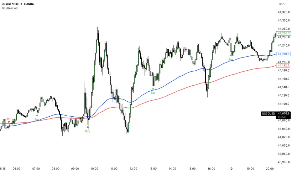
Fibs Has Lied 🌟 Fibs Has Lied - Indicator Overview 🌟
Designed for indices like US30, NQ, and SPX, this indicator highlights setups where price interacts with key EMA levels during specific trading sessions (default: 6:30–11:30 AM EST).
🌟 Key Features & Levels 🌟
🔹EMA Crossover Setups
The indicator uses the 100-period and 200-period EMAs to identify bullish and bearish setups:
- Bullish Setup: Triggers when the 100 EMA crosses above the 200 EMA, followed by two consecutive candles opening above the 100 EMA, with the low within a specified point distance (e.g., 20 points for US30).
- Bearish Setup: Triggers when the 100 EMA crosses below the 200 EMA, followed by two consecutive candles opening below the 100 EMA, with the high within the point distance.
- Signals are marked with green (buy) or red (sell) triangles and text, ensuring you don’t miss a setup. 📈
🔹 Reset Conditions for Re-Entries
After an initial setup, the indicator watches for “reset” opportunities:
- Buy Reset: If price moves below the 200 EMA after a bullish crossover, then returns with two consecutive candles where lows are above the 100 EMA (within point distance), a new buy signal is plotted.
- Sell Reset: If price moves above the 200 EMA after a bearish crossover, then returns with two consecutive candles where highs are below the 100 EMA (within point distance), a new sell signal is plotted.
This feature captures additional entries after liquidity grabs or fakeouts, aligning with ICT’s manipulation concepts. 🔄
🔹 Session-Based Filtering
Focus your trades during high-liquidity windows! The default session (6:30–11:30 AM EST, New York timezone) targets the London/NY overlap, where price often seeks liquidity or sets up for reversals. Toggle the time filter off for 24/7 signals if desired. 🕒
🔹Symbol-Specific Point Distance
Customizable entry zones based on your chosen index:
- US30: 20 points from the 100 EMA.
- NQ: 3 points from the 100 EMA.
- SPX: 2.5 points from the 100 EMA.
This ensures setups are tailored to the volatility of your market, maximizing relevance. 🎯
🔹 Market Structure Markers (Optional)
Visualize swing points with pivot-based labels:
- HH (Higher High): Signals uptrend continuation.
- HL (Higher Low): Indicates potential bullish support.
- LH (Lower High): Suggests weakening uptrend or reversal.
- LL (Lower Low): Points to downtrend continuation.
- Toggle these on/off to keep your chart clean while analyzing trend direction. 📊
🔹 EMA Visualization
Optionally plot the 100 EMA (blue) and 200 EMA (red) to see key levels where price reacts. These act as dynamic support/resistance, perfect for spotting liquidity pools or ICT’s Power of 3 setups. ⚖️
🌟 Customization Options 🌟
- Symbol Selection: Choose US30, NQ, or SPX to adjust point distance for entries.
- Time Filter: Enable/disable the 6:30–11:30 AM EST session to focus on high-liquidity periods.
- EMA Display: Toggle 100/200 EMAs on/off to reduce chart clutter.
- Market Structure: Show/hide HH/HL/LH/LL labels for cleaner analysis.
- Signal Markers: Green (buy) and red (sell) triangles with text are auto-plotted for easy identification.
🌟 Usage Tips 🌟
- Best Timeframes: Use on 3m for intraday scalping and 30m for swing trades.
- Combine with ICT Tools: Pair with order blocks, fair value gaps, or kill zones for stronger setups.
- Focus on Session: The default 6:30–11:30 AM EST session captures London/NY volatility—perfect for liquidity-driven moves.
- Avoid Overcrowding: Disable market structure or EMAs if you only want setup signals.
Sniper NAS100 Swiss Knife IndicatorSniper Trading System – Master Indicator
Description:
“Trade with the precision of the market makers themselves.”
The Sniper Trading System – Master Indicator is the crown jewel of institutional-level trading tools, engineered for those who demand perfect timing, deadly accuracy, and surgical execution in any market.
Designed by a 3× ASCAP Award-winning, multi–funded prop firm trader, this system fuses algorithmic precision with battle-tested price action logic, delivering an unmatched trading edge across Forex, Futures, Indices, and Crypto.
Core Features
Dealer Range Mapping – Auto-detects the hidden accumulation/distribution zones that drive market direction.
Multi-Standard Deviation Targets – Projected with gradient precision (+1 to +4 / -1 to -4) for scalps or swing holds.
12 AM Bias Candle Logic – Reveals the true daily directional bias before the herd even wakes up.
Liquidity Sweep Detection – Spots equal highs/lows & engineered stop hunts before the main move.
Kill Zone Time Windows – Pre-programmed with the London Session Sniper Hours & New York Precision Plays.
Multi-Timeframe RSI Filter – Filters false signals & highlights exhaustion points for sniper entries.
Dynamic Alerts – Fire real-time push, email, or webhook notifications for entry, exit, and confluence events.
How It Works
Identify Bias – Use the 12 AM candle + DXY/RSI overlays to confirm bullish or bearish control.
Wait for Liquidity Sweep – Let the market makers hunt stops; your job is to wait.
Execute at Kill Zones – Follow the preloaded precision entry times for God-tier sniper plays.
Ride to Target Zones – Exit at projected standard deviation levels for mathematically consistent profits.
Ideal For
Day Traders looking for clean entries and exits.

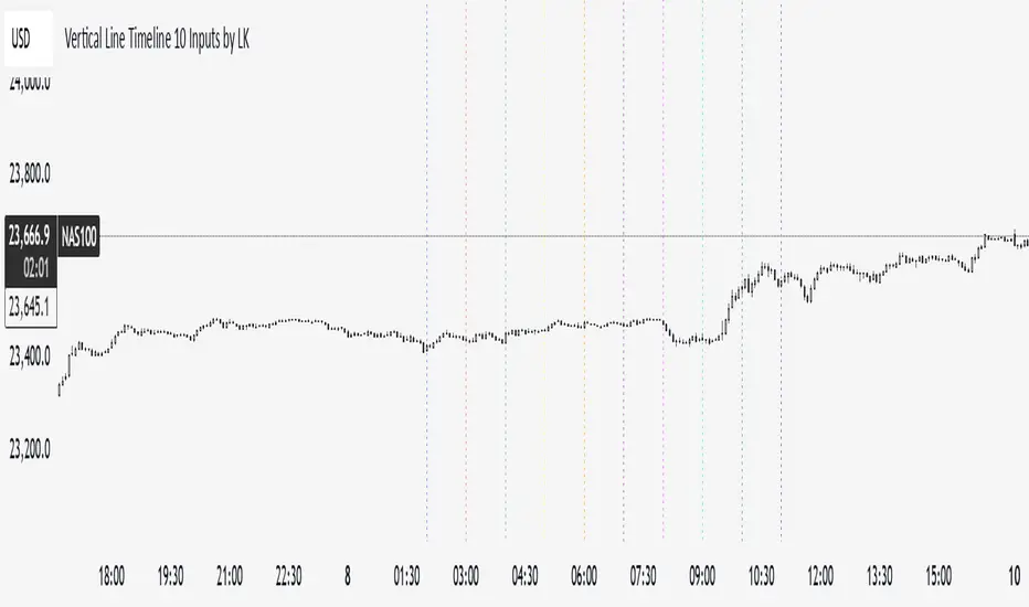
Vertical Line Timeline 10 Inputs by LK**Vertical Line Timeline (10 Inputs)**
This TradingView indicator plots vertical lines on your chart at up to **10 specific times of day**. You can define each time in **HH.MM format** (e.g., `9.30` for 9:30 AM). When the current bar’s time matches any of the defined times (based on the chart’s timezone), the indicator automatically draws a **full-height vertical line** at that bar.
**Features:**
* **Up to 10 custom time inputs** (HH.MM format)
* **Custom color** for each time marker
* **Adjustable line width** (1–6 px)
* **Solid or dotted style** toggle
* **Full-height vertical lines** (extend through the entire chart height)
* Works on any intraday timeframe where bar start times can match the defined times
* No labels or extra elements — clean and minimal display
**Use cases:**
* Marking important market sessions (e.g., London Open, New York Open, Asian Close)
* Highlighting personal trade execution windows
* Visual cues for strategy backtesting or time-based setups
Kelly Position Size CalculatorThis position sizing calculator implements the Kelly Criterion, developed by John L. Kelly Jr. at Bell Laboratories in 1956, to determine mathematically optimal position sizes for maximizing long-term wealth growth. Unlike arbitrary position sizing methods, this tool provides a scientifically solution based on your strategy's actual performance statistics and incorporates modern refinements from over six decades of academic research.
The Kelly Criterion addresses a fundamental question in capital allocation: "What fraction of capital should be allocated to each opportunity to maximize growth while avoiding ruin?" This question has profound implications for financial markets, where traders and investors constantly face decisions about optimal capital allocation (Van Tharp, 2007).
Theoretical Foundation
The Kelly Criterion for binary outcomes is expressed as f* = (bp - q) / b, where f* represents the optimal fraction of capital to allocate, b denotes the risk-reward ratio, p indicates the probability of success, and q represents the probability of loss (Kelly, 1956). This formula maximizes the expected logarithm of wealth, ensuring maximum long-term growth rate while avoiding the risk of ruin.
The mathematical elegance of Kelly's approach lies in its derivation from information theory. Kelly's original work was motivated by Claude Shannon's information theory (Shannon, 1948), recognizing that maximizing the logarithm of wealth is equivalent to maximizing the rate of information transmission. This connection between information theory and wealth accumulation provides a deep theoretical foundation for optimal position sizing.
The logarithmic utility function underlying the Kelly Criterion naturally embodies several desirable properties for capital management. It exhibits decreasing marginal utility, penalizes large losses more severely than it rewards equivalent gains, and focuses on geometric rather than arithmetic mean returns, which is appropriate for compounding scenarios (Thorp, 2006).
Scientific Implementation
This calculator extends beyond basic Kelly implementation by incorporating state of the art refinements from academic research:
Parameter Uncertainty Adjustment: Following Michaud (1989), the implementation applies Bayesian shrinkage to account for parameter estimation error inherent in small sample sizes. The adjustment formula f_adjusted = f_kelly × confidence_factor + f_conservative × (1 - confidence_factor) addresses the overconfidence bias documented by Baker and McHale (2012), where the confidence factor increases with sample size and the conservative estimate equals 0.25 (quarter Kelly).
Sample Size Confidence: The reliability of Kelly calculations depends critically on sample size. Research by Browne and Whitt (1996) provides theoretical guidance on minimum sample requirements, suggesting that at least 30 independent observations are necessary for meaningful parameter estimates, with 100 or more trades providing reliable estimates for most trading strategies.
Universal Asset Compatibility: The calculator employs intelligent asset detection using TradingView's built-in symbol information, automatically adapting calculations for different asset classes without manual configuration.
ASSET SPECIFIC IMPLEMENTATION
Equity Markets: For stocks and ETFs, position sizing follows the calculation Shares = floor(Kelly Fraction × Account Size / Share Price). This straightforward approach reflects whole share constraints while accommodating fractional share trading capabilities.
Foreign Exchange Markets: Forex markets require lot-based calculations following Lot Size = Kelly Fraction × Account Size / (100,000 × Base Currency Value). The calculator automatically handles major currency pairs with appropriate pip value calculations, following industry standards described by Archer (2010).
Futures Markets: Futures position sizing accounts for leverage and margin requirements through Contracts = floor(Kelly Fraction × Account Size / Margin Requirement). The calculator estimates margin requirements as a percentage of contract notional value, with specific adjustments for micro-futures contracts that have smaller sizes and reduced margin requirements (Kaufman, 2013).
Index and Commodity Markets: These markets combine characteristics of both equity and futures markets. The calculator automatically detects whether instruments are cash-settled or futures-based, applying appropriate sizing methodologies with correct point value calculations.
Risk Management Integration
The calculator integrates sophisticated risk assessment through two primary modes:
Stop Loss Integration: When fixed stop-loss levels are defined, risk calculation follows Risk per Trade = Position Size × Stop Loss Distance. This ensures that the Kelly fraction accounts for actual risk exposure rather than theoretical maximum loss, with stop-loss distance measured in appropriate units for each asset class.
Strategy Drawdown Assessment: For discretionary exit strategies, risk estimation uses maximum historical drawdown through Risk per Trade = Position Value × (Maximum Drawdown / 100). This approach assumes that individual trade losses will not exceed the strategy's historical maximum drawdown, providing a reasonable estimate for strategies with well-defined risk characteristics.
Fractional Kelly Approaches
Pure Kelly sizing can produce substantial volatility, leading many practitioners to adopt fractional Kelly approaches. MacLean, Sanegre, Zhao, and Ziemba (2004) analyze the trade-offs between growth rate and volatility, demonstrating that half-Kelly typically reduces volatility by approximately 75% while sacrificing only 25% of the growth rate.
The calculator provides three primary Kelly modes to accommodate different risk preferences and experience levels. Full Kelly maximizes growth rate while accepting higher volatility, making it suitable for experienced practitioners with strong risk tolerance and robust capital bases. Half Kelly offers a balanced approach popular among professional traders, providing optimal risk-return balance by reducing volatility significantly while maintaining substantial growth potential. Quarter Kelly implements a conservative approach with low volatility, recommended for risk-averse traders or those new to Kelly methodology who prefer gradual introduction to optimal position sizing principles.
Empirical Validation and Performance
Extensive academic research supports the theoretical advantages of Kelly sizing. Hakansson and Ziemba (1995) provide a comprehensive review of Kelly applications in finance, documenting superior long-term performance across various market conditions and asset classes. Estrada (2008) analyzes Kelly performance in international equity markets, finding that Kelly-based strategies consistently outperform fixed position sizing approaches over extended periods across 19 developed markets over a 30-year period.
Several prominent investment firms have successfully implemented Kelly-based position sizing. Pabrai (2007) documents the application of Kelly principles at Berkshire Hathaway, noting Warren Buffett's concentrated portfolio approach aligns closely with Kelly optimal sizing for high-conviction investments. Quantitative hedge funds, including Renaissance Technologies and AQR, have incorporated Kelly-based risk management into their systematic trading strategies.
Practical Implementation Guidelines
Successful Kelly implementation requires systematic application with attention to several critical factors:
Parameter Estimation: Accurate parameter estimation represents the greatest challenge in practical Kelly implementation. Brown (1976) notes that small errors in probability estimates can lead to significant deviations from optimal performance. The calculator addresses this through Bayesian adjustments and confidence measures.
Sample Size Requirements: Users should begin with conservative fractional Kelly approaches until achieving sufficient historical data. Strategies with fewer than 30 trades may produce unreliable Kelly estimates, regardless of adjustments. Full confidence typically requires 100 or more independent trade observations.
Market Regime Considerations: Parameters that accurately describe historical performance may not reflect future market conditions. Ziemba (2003) recommends regular parameter updates and conservative adjustments when market conditions change significantly.
Professional Features and Customization
The calculator provides comprehensive customization options for professional applications:
Multiple Color Schemes: Eight professional color themes (Gold, EdgeTools, Behavioral, Quant, Ocean, Fire, Matrix, Arctic) with dark and light theme compatibility ensure optimal visibility across different trading environments.
Flexible Display Options: Adjustable table size and position accommodate various chart layouts and user preferences, while maintaining analytical depth and clarity.
Comprehensive Results: The results table presents essential information including asset specifications, strategy statistics, Kelly calculations, sample confidence measures, position values, risk assessments, and final position sizes in appropriate units for each asset class.
Limitations and Considerations
Like any analytical tool, the Kelly Criterion has important limitations that users must understand:
Stationarity Assumption: The Kelly Criterion assumes that historical strategy statistics represent future performance characteristics. Non-stationary market conditions may invalidate this assumption, as noted by Lo and MacKinlay (1999).
Independence Requirement: Each trade should be independent to avoid correlation effects. Many trading strategies exhibit serial correlation in returns, which can affect optimal position sizing and may require adjustments for portfolio applications.
Parameter Sensitivity: Kelly calculations are sensitive to parameter accuracy. Regular calibration and conservative approaches are essential when parameter uncertainty is high.
Transaction Costs: The implementation incorporates user-defined transaction costs but assumes these remain constant across different position sizes and market conditions, following Ziemba (2003).
Advanced Applications and Extensions
Multi-Asset Portfolio Considerations: While this calculator optimizes individual position sizes, portfolio-level applications require additional considerations for correlation effects and aggregate risk management. Simplified portfolio approaches include treating positions independently with correlation adjustments.
Behavioral Factors: Behavioral finance research reveals systematic biases that can interfere with Kelly implementation. Kahneman and Tversky (1979) document loss aversion, overconfidence, and other cognitive biases that lead traders to deviate from optimal strategies. Successful implementation requires disciplined adherence to calculated recommendations.
Time-Varying Parameters: Advanced implementations may incorporate time-varying parameter models that adjust Kelly recommendations based on changing market conditions, though these require sophisticated econometric techniques and substantial computational resources.
Comprehensive Usage Instructions and Practical Examples
Implementation begins with loading the calculator on your desired trading instrument's chart. The system automatically detects asset type across stocks, forex, futures, and cryptocurrency markets while extracting current price information. Navigation to the indicator settings allows input of your specific strategy parameters.
Strategy statistics configuration requires careful attention to several key metrics. The win rate should be calculated from your backtest results using the formula of winning trades divided by total trades multiplied by 100. Average win represents the sum of all profitable trades divided by the number of winning trades, while average loss calculates the sum of all losing trades divided by the number of losing trades, entered as a positive number. The total historical trades parameter requires the complete number of trades in your backtest, with a minimum of 30 trades recommended for basic functionality and 100 or more trades optimal for statistical reliability. Account size should reflect your available trading capital, specifically the risk capital allocated for trading rather than total net worth.
Risk management configuration adapts to your specific trading approach. The stop loss setting should be enabled if you employ fixed stop-loss exits, with the stop loss distance specified in appropriate units depending on the asset class. For stocks, this distance is measured in dollars, for forex in pips, and for futures in ticks. When stop losses are not used, the maximum strategy drawdown percentage from your backtest provides the risk assessment baseline. Kelly mode selection offers three primary approaches: Full Kelly for aggressive growth with higher volatility suitable for experienced practitioners, Half Kelly for balanced risk-return optimization popular among professional traders, and Quarter Kelly for conservative approaches with reduced volatility.
Display customization ensures optimal integration with your trading environment. Eight professional color themes provide optimization for different chart backgrounds and personal preferences. Table position selection allows optimal placement within your chart layout, while table size adjustment ensures readability across different screen resolutions and viewing preferences.
Detailed Practical Examples
Example 1: SPY Swing Trading Strategy
Consider a professionally developed swing trading strategy for SPY (S&P 500 ETF) with backtesting results spanning 166 total trades. The strategy achieved 110 winning trades, representing a 66.3% win rate, with an average winning trade of $2,200 and average losing trade of $862. The maximum drawdown reached 31.4% during the testing period, and the available trading capital amounts to $25,000. This strategy employs discretionary exits without fixed stop losses.
Implementation requires loading the calculator on the SPY daily chart and configuring the parameters accordingly. The win rate input receives 66.3, while average win and loss inputs receive 2200 and 862 respectively. Total historical trades input requires 166, with account size set to 25000. The stop loss function remains disabled due to the discretionary exit approach, with maximum strategy drawdown set to 31.4%. Half Kelly mode provides the optimal balance between growth and risk management for this application.
The calculator generates several key outputs for this scenario. The risk-reward ratio calculates automatically to 2.55, while the Kelly fraction reaches approximately 53% before scientific adjustments. Sample confidence achieves 100% given the 166 trades providing high statistical confidence. The recommended position settles at approximately 27% after Half Kelly and Bayesian adjustment factors. Position value reaches approximately $6,750, translating to 16 shares at a $420 SPY price. Risk per trade amounts to approximately $2,110, representing 31.4% of position value, with expected value per trade reaching approximately $1,466. This recommendation represents the mathematically optimal balance between growth potential and risk management for this specific strategy profile.
Example 2: EURUSD Day Trading with Stop Losses
A high-frequency EURUSD day trading strategy demonstrates different parameter requirements compared to swing trading approaches. This strategy encompasses 89 total trades with a 58% win rate, generating an average winning trade of $180 and average losing trade of $95. The maximum drawdown reached 12% during testing, with available capital of $10,000. The strategy employs fixed stop losses at 25 pips and take profit targets at 45 pips, providing clear risk-reward parameters.
Implementation begins with loading the calculator on the EURUSD 1-hour chart for appropriate timeframe alignment. Parameter configuration includes win rate at 58, average win at 180, and average loss at 95. Total historical trades input receives 89, with account size set to 10000. The stop loss function is enabled with distance set to 25 pips, reflecting the fixed exit strategy. Quarter Kelly mode provides conservative positioning due to the smaller sample size compared to the previous example.
Results demonstrate the impact of smaller sample sizes on Kelly calculations. The risk-reward ratio calculates to 1.89, while the Kelly fraction reaches approximately 32% before adjustments. Sample confidence achieves 89%, providing moderate statistical confidence given the 89 trades. The recommended position settles at approximately 7% after Quarter Kelly application and Bayesian shrinkage adjustment for the smaller sample. Position value amounts to approximately $700, translating to 0.07 standard lots. Risk per trade reaches approximately $175, calculated as 25 pips multiplied by lot size and pip value, with expected value per trade at approximately $49. This conservative position sizing reflects the smaller sample size, with position sizes expected to increase as trade count surpasses 100 and statistical confidence improves.
Example 3: ES1! Futures Systematic Strategy
Systematic futures trading presents unique considerations for Kelly criterion application, as demonstrated by an E-mini S&P 500 futures strategy encompassing 234 total trades. This systematic approach achieved a 45% win rate with an average winning trade of $1,850 and average losing trade of $720. The maximum drawdown reached 18% during the testing period, with available capital of $50,000. The strategy employs 15-tick stop losses with contract specifications of $50 per tick, providing precise risk control mechanisms.
Implementation involves loading the calculator on the ES1! 15-minute chart to align with the systematic trading timeframe. Parameter configuration includes win rate at 45, average win at 1850, and average loss at 720. Total historical trades receives 234, providing robust statistical foundation, with account size set to 50000. The stop loss function is enabled with distance set to 15 ticks, reflecting the systematic exit methodology. Half Kelly mode balances growth potential with appropriate risk management for futures trading.
Results illustrate how favorable risk-reward ratios can support meaningful position sizing despite lower win rates. The risk-reward ratio calculates to 2.57, while the Kelly fraction reaches approximately 16%, lower than previous examples due to the sub-50% win rate. Sample confidence achieves 100% given the 234 trades providing high statistical confidence. The recommended position settles at approximately 8% after Half Kelly adjustment. Estimated margin per contract amounts to approximately $2,500, resulting in a single contract allocation. Position value reaches approximately $2,500, with risk per trade at $750, calculated as 15 ticks multiplied by $50 per tick. Expected value per trade amounts to approximately $508. Despite the lower win rate, the favorable risk-reward ratio supports meaningful position sizing, with single contract allocation reflecting appropriate leverage management for futures trading.
Example 4: MES1! Micro-Futures for Smaller Accounts
Micro-futures contracts provide enhanced accessibility for smaller trading accounts while maintaining identical strategy characteristics. Using the same systematic strategy statistics from the previous example but with available capital of $15,000 and micro-futures specifications of $5 per tick with reduced margin requirements, the implementation demonstrates improved position sizing granularity.
Kelly calculations remain identical to the full-sized contract example, maintaining the same risk-reward dynamics and statistical foundations. However, estimated margin per contract reduces to approximately $250 for micro-contracts, enabling allocation of 4-5 micro-contracts. Position value reaches approximately $1,200, while risk per trade calculates to $75, derived from 15 ticks multiplied by $5 per tick. This granularity advantage provides better position size precision for smaller accounts, enabling more accurate Kelly implementation without requiring large capital commitments.
Example 5: Bitcoin Swing Trading
Cryptocurrency markets present unique challenges requiring modified Kelly application approaches. A Bitcoin swing trading strategy on BTCUSD encompasses 67 total trades with a 71% win rate, generating average winning trades of $3,200 and average losing trades of $1,400. Maximum drawdown reached 28% during testing, with available capital of $30,000. The strategy employs technical analysis for exits without fixed stop losses, relying on price action and momentum indicators.
Implementation requires conservative approaches due to cryptocurrency volatility characteristics. Quarter Kelly mode is recommended despite the high win rate to account for crypto market unpredictability. Expected position sizing remains reduced due to the limited sample size of 67 trades, requiring additional caution until statistical confidence improves. Regular parameter updates are strongly recommended due to cryptocurrency market evolution and changing volatility patterns that can significantly impact strategy performance characteristics.
Advanced Usage Scenarios
Portfolio position sizing requires sophisticated consideration when running multiple strategies simultaneously. Each strategy should have its Kelly fraction calculated independently to maintain mathematical integrity. However, correlation adjustments become necessary when strategies exhibit related performance patterns. Moderately correlated strategies should receive individual position size reductions of 10-20% to account for overlapping risk exposure. Aggregate portfolio risk monitoring ensures total exposure remains within acceptable limits across all active strategies. Professional practitioners often consider using lower fractional Kelly approaches, such as Quarter Kelly, when running multiple strategies simultaneously to provide additional safety margins.
Parameter sensitivity analysis forms a critical component of professional Kelly implementation. Regular validation procedures should include monthly parameter updates using rolling 100-trade windows to capture evolving market conditions while maintaining statistical relevance. Sensitivity testing involves varying win rates by ±5% and average win/loss ratios by ±10% to assess recommendation stability under different parameter assumptions. Out-of-sample validation reserves 20% of historical data for parameter verification, ensuring that optimization doesn't create curve-fitted results. Regime change detection monitors actual performance against expected metrics, triggering parameter reassessment when significant deviations occur.
Risk management integration requires professional overlay considerations beyond pure Kelly calculations. Daily loss limits should cease trading when daily losses exceed twice the calculated risk per trade, preventing emotional decision-making during adverse periods. Maximum position limits should never exceed 25% of account value in any single position regardless of Kelly recommendations, maintaining diversification principles. Correlation monitoring reduces position sizes when holding multiple correlated positions that move together during market stress. Volatility adjustments consider reducing position sizes during periods of elevated VIX above 25 for equity strategies, adapting to changing market conditions.
Troubleshooting and Optimization
Professional implementation often encounters specific challenges requiring systematic troubleshooting approaches. Zero position size displays typically result from insufficient capital for minimum position sizes, negative expected values, or extremely conservative Kelly calculations. Solutions include increasing account size, verifying strategy statistics for accuracy, considering Quarter Kelly mode for conservative approaches, or reassessing overall strategy viability when fundamental issues exist.
Extremely high Kelly fractions exceeding 50% usually indicate underlying problems with parameter estimation. Common causes include unrealistic win rates, inflated risk-reward ratios, or curve-fitted backtest results that don't reflect genuine trading conditions. Solutions require verifying backtest methodology, including all transaction costs in calculations, testing strategies on out-of-sample data, and using conservative fractional Kelly approaches until parameter reliability improves.
Low sample confidence below 50% reflects insufficient historical trades for reliable parameter estimation. This situation demands gathering additional trading data, using Quarter Kelly approaches until reaching 100 or more trades, applying extra conservatism in position sizing, and considering paper trading to build statistical foundations without capital risk.
Inconsistent results across similar strategies often stem from parameter estimation differences, market regime changes, or strategy degradation over time. Professional solutions include standardizing backtest methodology across all strategies, updating parameters regularly to reflect current conditions, and monitoring live performance against expectations to identify deteriorating strategies.
Position sizes that appear inappropriately large or small require careful validation against traditional risk management principles. Professional standards recommend never risking more than 2-3% per trade regardless of Kelly calculations. Calibration should begin with Quarter Kelly approaches, gradually increasing as comfort and confidence develop. Most institutional traders utilize 25-50% of full Kelly recommendations to balance growth with prudent risk management.
Market condition adjustments require dynamic approaches to Kelly implementation. Trending markets may support full Kelly recommendations when directional momentum provides favorable conditions. Ranging or volatile markets typically warrant reducing to Half or Quarter Kelly to account for increased uncertainty. High correlation periods demand reducing individual position sizes when multiple positions move together, concentrating risk exposure. News and event periods often justify temporary position size reductions during high-impact releases that can create unpredictable market movements.
Performance monitoring requires systematic protocols to ensure Kelly implementation remains effective over time. Weekly reviews should compare actual versus expected win rates and average win/loss ratios to identify parameter drift or strategy degradation. Position size efficiency and execution quality monitoring ensures that calculated recommendations translate effectively into actual trading results. Tracking correlation between calculated and realized risk helps identify discrepancies between theoretical and practical risk exposure.
Monthly calibration provides more comprehensive parameter assessment using the most recent 100 trades to maintain statistical relevance while capturing current market conditions. Kelly mode appropriateness requires reassessment based on recent market volatility and performance characteristics, potentially shifting between Full, Half, and Quarter Kelly approaches as conditions change. Transaction cost evaluation ensures that commission structures, spreads, and slippage estimates remain accurate and current.
Quarterly strategic reviews encompass comprehensive strategy performance analysis comparing long-term results against expectations and identifying trends in effectiveness. Market regime assessment evaluates parameter stability across different market conditions, determining whether strategy characteristics remain consistent or require fundamental adjustments. Strategic modifications to position sizing methodology may become necessary as markets evolve or trading approaches mature, ensuring that Kelly implementation continues supporting optimal capital allocation objectives.
Professional Applications
This calculator serves diverse professional applications across the financial industry. Quantitative hedge funds utilize the implementation for systematic position sizing within algorithmic trading frameworks, where mathematical precision and consistent application prove essential for institutional capital management. Professional discretionary traders benefit from optimized position management that removes emotional bias while maintaining flexibility for market-specific adjustments. Portfolio managers employ the calculator for developing risk-adjusted allocation strategies that enhance returns while maintaining prudent risk controls across diverse asset classes and investment strategies.
Individual traders seeking mathematical optimization of capital allocation find the calculator provides institutional-grade methodology previously available only to professional money managers. The Kelly Criterion establishes theoretical foundation for optimal capital allocation across both single strategies and multiple trading systems, offering significant advantages over arbitrary position sizing methods that rely on intuition or fixed percentage approaches. Professional implementation ensures consistent application of mathematically sound principles while adapting to changing market conditions and strategy performance characteristics.
Conclusion
The Kelly Criterion represents one of the few mathematically optimal solutions to fundamental investment problems. When properly understood and carefully implemented, it provides significant competitive advantage in financial markets. This calculator implements modern refinements to Kelly's original formula while maintaining accessibility for practical trading applications.
Success with Kelly requires ongoing learning, systematic application, and continuous refinement based on market feedback and evolving research. Users who master Kelly principles and implement them systematically can expect superior risk-adjusted returns and more consistent capital growth over extended periods.
The extensive academic literature provides rich resources for deeper study, while practical experience builds the intuition necessary for effective implementation. Regular parameter updates, conservative approaches with limited data, and disciplined adherence to calculated recommendations are essential for optimal results.
References
Archer, M. D. (2010). Getting Started in Currency Trading: Winning in Today's Forex Market (3rd ed.). John Wiley & Sons.
Baker, R. D., & McHale, I. G. (2012). An empirical Bayes approach to optimising betting strategies. Journal of the Royal Statistical Society: Series D (The Statistician), 61(1), 75-92.
Breiman, L. (1961). Optimal gambling systems for favorable games. In J. Neyman (Ed.), Proceedings of the Fourth Berkeley Symposium on Mathematical Statistics and Probability (pp. 65-78). University of California Press.
Brown, D. B. (1976). Optimal portfolio growth: Logarithmic utility and the Kelly criterion. In W. T. Ziemba & R. G. Vickson (Eds.), Stochastic Optimization Models in Finance (pp. 1-23). Academic Press.
Browne, S., & Whitt, W. (1996). Portfolio choice and the Bayesian Kelly criterion. Advances in Applied Probability, 28(4), 1145-1176.
Estrada, J. (2008). Geometric mean maximization: An overlooked portfolio approach? The Journal of Investing, 17(4), 134-147.
Hakansson, N. H., & Ziemba, W. T. (1995). Capital growth theory. In R. A. Jarrow, V. Maksimovic, & W. T. Ziemba (Eds.), Handbooks in Operations Research and Management Science (Vol. 9, pp. 65-86). Elsevier.
Kahneman, D., & Tversky, A. (1979). Prospect theory: An analysis of decision under risk. Econometrica, 47(2), 263-291.
Kaufman, P. J. (2013). Trading Systems and Methods (5th ed.). John Wiley & Sons.
Kelly Jr, J. L. (1956). A new interpretation of information rate. Bell System Technical Journal, 35(4), 917-926.
Lo, A. W., & MacKinlay, A. C. (1999). A Non-Random Walk Down Wall Street. Princeton University Press.
MacLean, L. C., Sanegre, E. O., Zhao, Y., & Ziemba, W. T. (2004). Capital growth with security. Journal of Economic Dynamics and Control, 28(4), 937-954.
MacLean, L. C., Thorp, E. O., & Ziemba, W. T. (2011). The Kelly Capital Growth Investment Criterion: Theory and Practice. World Scientific.
Michaud, R. O. (1989). The Markowitz optimization enigma: Is 'optimized' optimal? Financial Analysts Journal, 45(1), 31-42.
Pabrai, M. (2007). The Dhandho Investor: The Low-Risk Value Method to High Returns. John Wiley & Sons.
Shannon, C. E. (1948). A mathematical theory of communication. Bell System Technical Journal, 27(3), 379-423.
Tharp, V. K. (2007). Trade Your Way to Financial Freedom (2nd ed.). McGraw-Hill.
Thorp, E. O. (2006). The Kelly criterion in blackjack sports betting, and the stock market. In L. C. MacLean, E. O. Thorp, & W. T. Ziemba (Eds.), The Kelly Capital Growth Investment Criterion: Theory and Practice (pp. 789-832). World Scientific.
Van Tharp, K. (2007). Trade Your Way to Financial Freedom (2nd ed.). McGraw-Hill Education.
Vince, R. (1992). The Mathematics of Money Management: Risk Analysis Techniques for Traders. John Wiley & Sons.
Vince, R., & Zhu, H. (2015). Optimal betting under parameter uncertainty. Journal of Statistical Planning and Inference, 161, 19-31.
Ziemba, W. T. (2003). The Stochastic Programming Approach to Asset, Liability, and Wealth Management. The Research Foundation of AIMR.
Further Reading
For comprehensive understanding of Kelly Criterion applications and advanced implementations:
MacLean, L. C., Thorp, E. O., & Ziemba, W. T. (2011). The Kelly Capital Growth Investment Criterion: Theory and Practice. World Scientific.
Vince, R. (1992). The Mathematics of Money Management: Risk Analysis Techniques for Traders. John Wiley & Sons.
Thorp, E. O. (2017). A Man for All Markets: From Las Vegas to Wall Street. Random House.
Cover, T. M., & Thomas, J. A. (2006). Elements of Information Theory (2nd ed.). John Wiley & Sons.
Ziemba, W. T., & Vickson, R. G. (Eds.). (2006). Stochastic Optimization Models in Finance. World Scientific.

Defense Mode Dashboard ProWhat it is
A one‑look market regime dashboard for ES, NQ, YM, RTY, and SPY that tells you when to play defense, when you might have an offense cue, and when to chill. It blends VIX, VIX term structure, ATR 5 over 60, and session gap signals with clean alerts and a compact table you can park anywhere.
Why traders like it
Because it filters out the noise. Regime first, tactics second. You avoid trading size into landmines and lean in when volatility cooperates.
What it measures
Volatility stress with VIX level and VIX vs 20‑SMA
Term structure using VX1 vs VX2 with two modes
Diff mode: VX1 minus VX2
Ratio mode: VX1 divided by VX2
Realized volatility using ATR5 over ATR60 with optional smoothing
Session risk from RTH opening gaps and overnight range, normalized by ATR
How to use in 30 seconds
Pick a preset in the inputs. ES, NQ, YM, RTY, SPY are ready.
Leave thresholds at defaults to start.
Add one TradingView alert using “Any alert() function call”.
Trade smaller or stand aside when the header reads DEFENSE ON. Consider leaning in only when you see OFFENSE CUE and your playbook agrees.
Defaults we recommend
VIX triggers: 22 and 1.25× the 20‑SMA
Term mode: Diff with tolerance 0.00. Use Ratio at 1.00+ for choppier markets
ATR 5/60 defense: 1.25. Offense cue: 0.85 or lower
ATR smoothing: 1. Try 2 to 3 if you want fewer flips
Gap mode: RTH. Turn Both on if you want ON range to count too
RTH wild gap: 0.60× ATR5. ON wild range: 0.80× ATR5
Alert cadence: Once per RTH session
Snooze: Quick snooze first 30 minutes on. Fire on snooze exit off, unless you really want the catch‑up ping
New since the last description
Multi‑asset presets set symbols and RTH windows for ES, NQ, YM, RTY, SPY
Term ratio mode with near‑flat warning when ratio is between 1.00 and your trigger
ATR smoothing for the 5 over 60 ratio
RTH keying for cadence, so “Once per RTH session” behaves like a trader expects
Snooze upgrades with quick snooze tied to the first N minutes of RTH and an optional fire‑on‑snooze‑exit
Compact title merge and user color controls for labels, values, borders, and background
Exposed series for integrations: DefenseOn(1=yes) and OffenseCue(1=yes)
Debug toggle to visualize gap points, ON range, and term readings
Stronger NA handling with a clear “No core data” row when feeds are missing
Notes
Dynamic alerts require “Any alert() function call”.
Works on any chart timeframe. Daily reads and 1‑minute anchors handle the regime logic.

Period Highlighter ProPeriod Highlighter Pro is a versatile Pine Script indicator designed to visually highlight specific time periods on your TradingView charts, making it easier to analyze seasonal patterns, trading sessions, or specific weekdays. With customizable settings for months, weekdays, or intraday time ranges, this tool adapts to your trading strategy, allowing you to focus on key periods with precision.
Features
Flexible Highlight Modes: Choose from three modes to highlight:
Month Range: Highlight specific months or a range (e.g., March to June) for seasonal analysis.
Weekday Range: Highlight specific weekdays (e.g., Mondays or Monday to Wednesday) for weekly pattern analysis.
Time Range: Highlight daily time windows (e.g., 15:30–22:00) for intraday session analysis, restricted to weekdays.
Customizable Timezone: Set any IANA timezone (e.g., America/New_York, Europe/London) or UTC offset to align highlights with your preferred market hours.
Historical Range Control: Define how far back to apply highlights with options for years (Month Range), weeks (Weekday Range), or days (Time Range).
Visual Customization: Choose your highlight color to match your chart style.
User-Friendly Inputs: Intuitive dropdowns and tooltips guide you through configuring each mode, ensuring only relevant settings are adjusted.
How It Works
Select a highlight mode and configure the corresponding settings:
Month Range: Pick a start month and an optional end month (or "Disabled" for a single month) and set the number of years back.
Weekday Range: Choose a start weekday and an optional end weekday (or "Disabled" for a single day) and set the number of weeks back.
Time Range: Specify a start and end time (24-hour format) and the number of weekdays back. The indicator then applies a semi-transparent background color to chart bars that meet your criteria, making it easy to spot relevant periods.
Use Cases
Seasonal Traders: Highlight specific months to analyze recurring market patterns.
Day Traders: Focus on active trading sessions (e.g., New York open) with precise time range highlighting.
Weekly Pattern Analysts: Isolate specific weekdays to study price behavior.
Global Traders: Adjust for any timezone to align with your market of interest.
Why Use Period Highlighter Pro?
This indicator simplifies time-based analysis by providing a clear visual overlay for your chosen periods. Whether you're studying historical trends or focusing on specific trading hours, Period Highlighter Pro offers the flexibility and precision to enhance your chart analysis.
Licensed under the Mozilla Public License 2.0.
GTrader-ICT All In One-Comumnity VersionMeet the **GTrader-ICT All In One **, a comprehensive toolkit designed to integrate key Inner Circle Trader (ICT) concepts directly onto your chart. This powerful overlay indicator consolidates multiple essential tools, streamlining your technical analysis and helping you identify key temporal and price-based events.
📚 References & Inspiration
This indicator stands on the shoulders of giants. With the help of **tradeforopp** and **LuxAlgo**. The concepts and some implementation details were referenced from the following excellent, publicly available scripts:
ICT Killzones: The session drawing and pivot logic is adapted from tradeforopp
ICT Macros: The macro detection and plotting functionality is inspired by the work of Lux Algo , particularly their widely-used indicators covering ICT concepts.
🎯 Core Features
* **ICT Killzones:** Visualize critical trading sessions with customizable boxes. You can easily toggle and style the **Asia**, **London**, and **New York (AM, Lunch, PM)** sessions to focus on the liquidity and volatility that matter most to your strategy.
* Fully customizable session times and colors.
* Timezone support to align sessions with your local or preferred trading time (defaults to `America/New_York`).
* **ICT Macros:** Automatically identify and plot specific, short-duration time windows where institutional algorithms are known to be active (e.g., `09:50-10:10`, `14:50-15:10`, etc.).
* Plots the high/low range of the macro, providing clear levels of interest.
* Utilizes 1-minute data for precision, even when viewing on 3-minute or 5-minute charts.
📚 Optimization over the other original indicators
We add the custom input for macros session, users just need to input the from/to hour: minute format, and they will be converted into session objects in pinescript
The macro draws function is optimized, removing redundant draws, leading to better performance
Add "Distance from Macro Line to Chart" option
Add "Session Drawings Limit" for better performance
⚠️ Notes on TradingView Warnings
You may encounter some warnings from TradingView when using this script. These are generally expected due to the script's advanced, event-driven nature:
1. **Function Call Consistency:** The function 'box.new' should be called on each calculation for consistency, which may appear. This happens because drawing elements (like session boxes) are intentionally created only on the *first bar* of a new session, not on every single bar. This is a necessary design choice for performance and to prevent duplicate drawings.
2. **Potential for Repainting/Slow Load:** The **Macro** feature uses the `request.security_lower_tf()` function to get accurate 1-minute data. This can trigger warnings about performance or slow loading times. This is a known trade-off for achieving the precision required for the feature.

Silver BulletSilver Bullet is a trading tool built for finding cleaner, higher-probability setups. It focuses on key windows of market movement and adds helpful tools like daily range levels and candlestick patterns.
Whether you’re trading breakouts or reversals, Silver Bullet gives you a clearer view of the market and more confidence in your setups.
⸻
🔹 Trading Setup #1: Macro Time
The Macro Time setting offers two modes: Macro Bullet and Silver Bullet. Both help traders focus on specific times when the market tends to deliver clean moves.
• Macro Bullet is based on the high and low of a full macro session. It automatically detects the session’s range and bias, then offers optimal entries for either Long or Short setups. Once the session resolves, it provides Fibonacci-based levels for entry, target, and stop loss.
• Silver Bullet is based on ICT concepts and focuses on the hourly range for London, NY AM, and NY PM sessions. It’s designed for quick time blocks and highlights key levels as the session unfolds.
To use this setup, set Macro Time to “ICT Sessions” and select your preferred mode under Bullet Mode.
⸻
🔹 Trading Setup #2: Daily Range
Enable Daily Range to draw Fibonacci levels based on either the previous day’s candle or the current day’s developing range. These levels help you identify potential support, resistance, and midpoint zones throughout the day.
With the current day’s range, levels automatically update in real time as new highs or lows form — keeping your chart aligned with evolving price action.
⸻
🔹 Trading Setup #3: Candlestick Patterns
Turn on Candlestick Patterns to automatically highlight clean reversal signals such as Hammers, Hanging Men, Shooting Stars, and Tweezers. Each pattern is detected using specific criteria and trend filters to reduce noise and improve reliability. They work especially well as confirmation signals around key levels or session zones.
Silver Bullet brings structure, clarity, and precision to your intraday trading. By combining time-based bias, price action levels, and pattern recognition, it helps you trade with purpose — not guesswork. Use one setup or combine all three for a complete view of the market, tailored to your style and session of choice.

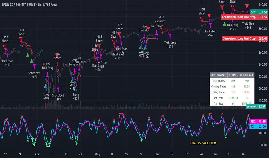
Strategy Chameleon [theUltimator5]Have you ever looked at an indicator and wondered to yourself "Is this indicator actually profitable?" Well now you can test it out for yourself with the Strategy Chameleon!
Strategy Chameleon is a versatile, signal-agnostic trading strategy designed to adapt to any external indicator or trading system. Like a chameleon changes colors to match its environment, this strategy adapts to match any buy/sell signals you provide, making it the ultimate backtesting and automation tool for traders who want to test multiple strategies without rewriting code.
🎯 Key Features
1) Connects ANY external indicator's buy/sell signals
Works with RSI, MACD, moving averages, custom indicators, or any Pine Script output
Simply connect your indicator's signal output to the strategy inputs
2) Multiple Stop Loss Types:
Percentage-based stops
ATR (Average True Range) dynamic stops
Fixed point stops
3) Advanced Trailing Stop System:
Percentage trailing
ATR-based trailing
Fixed point trailing
4) Flexible Take Profit Options:
Risk:Reward ratio targeting
Percentage-based profits
ATR-based profits
Fixed point profits
5) Trading Direction Control
Long Only - Bull market strategies
Short Only - Bear market strategies
Both - Full market strategies
6) Time-Based Filtering
Optional trading session restrictions
Customize active trading hours
Perfect for day trading strategies
📈 How It Works
Signal Detection: The strategy monitors your connected buy/sell signals
Entry Logic: Executes trades when signals trigger during valid time periods
Risk Management: Automatically applies your chosen stop loss and take profit levels
Trailing System: Dynamically adjusts stops to lock in profits
Performance Tracking: Real-time statistics table showing win rate and performance
⚙️ Setup Instructions
0) Add indicator you want to test, then add the Strategy to your chart
Connect Your Signals:
imgur.com
Go to strategy settings → Signal Sources
1) Set "Buy Signal Source" to your indicator's buy output
2) Set "Sell Signal Source" to your indicator's sell output
3) Choose table position - This simply changes the table location on the screen
4) Set trading direction preference - Buy only? Sell only? Both directions?
imgur.com
5) Set your preferred stop loss type and level
You can set the stop loss to be either percentage based or ATR and fully configurable.
6) Enable trailing stops if desired
imgur.com
7) Configure take profit settings
8) Toggle time filter to only consider specific time windows or trading sessions.
🚀 Use Cases
Test various indicators to determine feasibility and/or profitability.
Compare different signal sources quickly
Validate trading ideas with consistent risk management
Portfolio Management
Apply uniform risk management across different strategies
Standardize stop loss and take profit rules
Monitor performance consistently
Automation Ready
Built-in alert conditions for automated trading
Compatible with trading bots and webhooks
Easy integration with external systems
⚠️ Important Notes
This strategy requires external signals to function
Default settings use 10% of equity per trade
Pyramiding is disabled (one position at a time)
Strategy calculates on bar close, not every tick
🔗 Integration Examples
Works perfectly with:
RSI strategies (connect RSI > 70 for sells, RSI < 30 for buys)
Moving average crossovers
MACD signal line crosses
Bollinger Band strategies
Custom oscillators and indicators
Multi-timeframe strategies
📋 Default Settings
Position Size: 10% of equity
Stop Loss: 2% percentage-based
Trailing Stop: 1.5% percentage-based (enabled)
Take Profit: Disabled (optional)
Trade Direction: Both long and short
Time Filter: Disabled
Institutional Sessions Overlay (Asia/London/NY)Institutional Sessions Overlay is a professional TradingView indicator that visually highlights the main trading sessions (Asia, London, and New York) directly on your chart.
Customizable: Easily adjust session start and end times (including minutes) for each market.
Timezone Alignment: Shift session boxes using the timezone offset parameter so sessions match your chart’s timezone exactly.
Clear Visuals: Colored boxes and optional labels display session opens and closes for fast institutional market structure reference.
Toggle Labels: Show or hide session open/close labels with a single click for a clean or detailed look.
Intuitive UI: User-friendly grouped settings for efficient configuration.
This tool is designed for day traders, institutional traders, and anyone who wants to instantly recognize global session timing and ranges for SMC, ICT, and other session-based strategies.
How to use:
Set your chart to your local timezone.
Use the "Session timezone offset" setting if session boxes do not match actual session opens on your chart.
Adjust the hours and minutes for each session as needed.
Enable or disable labels in the “Display” settings group.
Tip: Use the overlay to spot session highs and lows, volatility windows, and institutional liquidity sweeps.
