mForex - Keltner channel + EMA Scalping systemTransaction setup parameters
Time frame: M5, M15
Currency pair: EUR / USD , GPB / USD
Transaction: London, USA
Number of orders / day: 10 - 15 orders
Trading strategies
=== BUY ===
Candles close on the upper Keltner
EMA10 crosses the upper Keltner range from below
Stop loss in the middle band or up to 12 pips
Profit target: 15-25 pips
=== SELL ===
Candles close below Keltner below
EMA10 crosses the Keltner range below from above
Stop loss in the middle band or up to 12 pips
Profit target: 15-25 pips
在腳本中搜尋"汇丰股票25"

Vertical Horizontal Moving Average [AneoPsy & alexgrover] Moving average adapting to the strength of the trend, this is made possible by using the square of the vertical-horizontal filter as a smoothing factor. Alerts are included with two different types of conditions available to the user.
Settings
Length : Period of the moving average
Src : Input data for the indicator
Alerts : Types of conditions to be used in the alerts, when set to "VHMA Direction Change" alerts are triggered once the VHMA is either rising or declining, else the alerts are based on the crosses between Src and the VHMA
Usage
The VHMA can be used as a fast or slow-moving average in a moving average crossover system, or as input for other indicators.
VHMA of with length = 25 and sma with length = 200.
VHMA with length = 25 used as input for the RSI with length = 14.
Details
The vertical-horizontal filter is a measure of the strength of the trend and lay in a (0,1) range, to calculate it you just need to divide the rolling range over with the rolling sum of the absolute price changes, squaring the result allow to get lower results with higher values of length .
Squared vertical horizontal filter with length = 50, the value is low when the market is ranging and high when trending.
To set the alerts go in the alert panel, click on create alert, and select VHMA in "condition", choose between the buy or sell alert. If Src = closing price or another indicator dependant on the closing price select in options "once per bar close", if the indicator using the opening or lagged closing prices values as input select "One per bar" instead.
Thanks
Thanks to AneoPsy for adding the color change, the idea to use two kinds of conditions for the alert, and for its feedback, you can follow him
www.tradingview.com
and finally thanks to you for reading and for your support, only one last script left for the month, then we'll start July with some pretty interesting indicators, I hope you'll like them ^^/

Sto RSI and kijun-sen line to determine and follow the trend This script uses 25-75 treshold of stochastic RSI with the help of kijun-sen as confirmation, to find entry points to any trend either newly developed or an established one. I just realized it on the 1 hour SPX chart. Sure it can be used on other symbols. Crossing above/below 25/75 line of sto RSI is considered as buy/sell signal. Signals are evaluated whether price be above/below kijun-sen line. If a sell signal below kijun-sen is generated it is a continuation signal for downtrend, otherwise it is a countertrend signal (maybe a signal for a new downtrend). A countertrend signal must be evaluated carefully and only accepted in the right side of kijun-sen. e.g entering a sell signal generated above kijun-sen should be accepted only below the kijun-sen, vice-versa.

Terminal : USD Based Stock Markets Change (%)Hello.
This script is a simple USD Based Stock Markets Change (%) Data Terminal.
You can also set the period to look back manually in the menu.
In this way, an idea can be obtained about Countries' Stock Markets.
And you can observe the stock exchanges of relatively positive and negative countries from others.
Features
Value changes on a percentage basis (%)
Stock exchange values are calculated in dollar terms.
Due to the advantage of movement, future data were chosen instead of spot values on the required instruments.
Stock Markets
Usa : S&P 500 Futures
Japan: Nikkei 225 Futures
England: United Kingdom ( FTSE ) 100
Australia: Australia 200
Canada: S&P / TSX Composite
Switzerland: Swiss Market Index
New Zealand: NZX 50 Index
China: SSE Composite (000001)
Denmark: OMX Copenhagen 25 Index
Hong-Kong: Hang Seng Index Futures
India: Nifty 50
Norway: Oslo Bors All Share Index
Russia: MOEX Russia Index
Sweden: OMX Stockholm Index
Singapore: Singapore 30
Turkey: BIST 100
South Africa: South Africa Top 40 Index
Spain: IBEX 35
France: CAC 40
Italy: FTSE MIB Index
Netherlands: Netherlands 25
Germany : DAX
Regards.

Bull Club BiasThe script intends to eliminate noise from the chart. It uses a combination of multiple indicators into 1.
For long bias:
Close is greater than the ADX
15 Period EMA on close is greater than SMA on high
13 period RSI is greater than 25 periods RSI
MACD is greater than 0
For short bias:
Close is lower than the ADX
15 Period EMA on close is lower than SMA on high
13 period RSI is lower than 25 periods RSI
MACD is lower than 0
For every other combination, it is a range-bound bias. NSE:BANKNIFTY
A green background indicates long bias
A Red background indicates short bias
An Orange background indicates range-bound bias

Easy Directional Movement IndexNothing more than a graphical tweak for the integrated Directional movement index (DMI). The purpose is to make the reading of the DMI easier and more immediate.
The area between DI+ and DI- is filled, and the indicator's range in divided into 4 sections, each of them representing a different price tendency:
- When ADX line is inside the red colored area (0-25), the market is in a ranging phase.
- When inside the aqua colored area (25-50), there is a trend.
- When inside the blue colored area (50-75), there is a strong trend
- When inside the navy colored area (75-100), there is an extremely strong trend.
However keep in mind that these are default levels that may be not always significant. You can change them from the script settings as you prefer, to better tweak your analysis.
Please support my work and follow me if you like my scripts. Many more of them are coming in the future.
@Bezzus

Ichimoku with Correct DisplacementThe default Ichimoku Cloud by TradingView is strange. The kumo is only displaced 25 periods forward, and the chikou is displaced 25 periods back. This is because TradingView had the correct value for displacement (26), but they decided to subtract this displacement by 1 when actually drawing the kumo and add 1 when drawing the chikou. This script fixes this and allows for easier customization of each line in the Ichimoku.

MACD At Scales with AlertsI use the horizontal scale lines on the MACD indicator as part of my scalping strategy along with other indicators like RSI/EMA and Market Cipher B when trading BTC
I am looking for a cross above or below the 12.5 and 25 horizontal scale lines, along with lining up other indicators
I set my alerts on the 5 min TF and look to the 15 and 30 min TF's for further confirmation.
I have find the scale lines to be very useful for visual reference of the crosses, above/below 25 lines is mostly a safer trade, crosses above/below 12.5 lines can have more risk, crosses between 0 baseline and 12.5 can have a higher return but have much more risk.
Don't ever use just this indicator by itself, you must always have at least 2 indicators running
This is an example of the TF's not lining up, so a entry here would be high risk
This is an example of the TF's lining up, so a entry here would be less risk
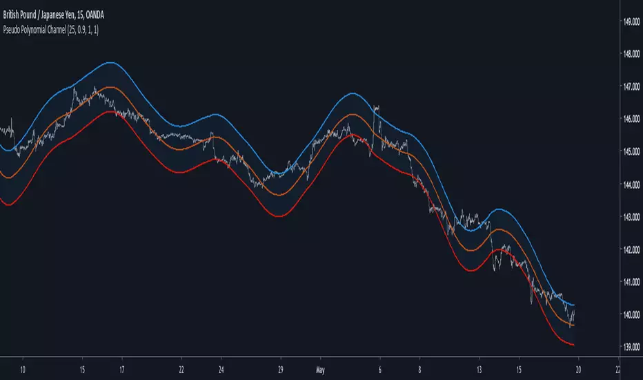
Pseudo Polynomial ChannelIntroduction
Back when i started using pine i made a script called periodic channel who aimed to rescale an average correlated sine wave to the price...don't worked very well. So i tried to fix problems induced by the indicator without much success, i had to redo it from scratch while abandoning the idea of rescaling correlated smooth functions to the price, at that time i also received requests regarding polynomial channel, some plateformes included this indicator, this led me to the idea to estimate it in order to both respond to the periodic channel problems and the requests i received, i have tried many many things and recently i tweaked a linear extrapolation to have an approximation.
Linear Extrapolation To Pseudo Polynomial Regression
I could be wrong but a polynomial regression must use constant parameters in order to provide a really smooth output, at least constant for a set of time. The moving averages forms (Savitzky-Golay moving average) who smooth polynomials across a window to the data don't have such smoothness, so how to estimate a polynomial regression while having a parameter providing control over the smoothness, a response to this is by using a recursive linear extrapolation. I posted a linear extrapolation indicator long ago, i used the same formula while adding a function to morph the output and the input in the form of :
morph * output + (1-morph) * input
How can this provide an estimate of a polynomial regression ? Well i'm not even sure myself but if you use the output as input (morph = 1) for the linear extrapolation function you should get a rough estimate of a line, this is what i thought at first and it proved to be right
Based on this observation i thought that it would be possible to get polynomial results by lowering morph, and as expected it worked well but showed a periodic pattern, this is why i smooth k in line 10.
0.9 for morph work well, higher values create sometimes smoother results but damage heavily the estimation.
Parameters
Morph have been introduced earlier, it control the amount of output and input the linear extrapolation should process, lower values create rougher but more stables results, if you see that the estimation is going nuts lower morph or change length, also lower length if you increase morph .
High overshoot, morph to 0.8 can help have a better estimation at the cost of less smoothness.
Length control the indicator smoothing, this parameter differ heavily from other filters, therefore low values can create mid/long term smoothing, it can also depend on which market instrument you are applying it, so there are no fixed optimal length.
Mult control how spread the bands are, to do so mult multiply the cumulative mean error, you can change this error measurement by anything you want like standard deviation/atr/range but take into account that you may create a separate parameter to control the error instead of length . Mult can be a float and like length can have different optimal values depending on the market the indicator is applied to.
Flatten do exactly what is name imply, it flatten the overall output to have a better estimation, can be a float. The result is less smooth.
Flatten = 2
More Exemples
BTCUSD length = 25 and mult = 4
XPDUSD length = 25 and mult = 1
ALPHABET length = 6 and morph = 0.99
Conclusion
I tried to estimate a polynomial channel by using recursion in the linear extrapolation function. This build is way more stable than the periodic channel but its still a bit inaccurate in my opinion. I hope this code can still help someone build something really nice, if so share your results :)
I apologize for those expecting a legit polynomial channel build but i really don't know how to do that, as i said parameters for the regression must be constants, i hope it still fine :)
Thanks for reading !
Modified Gann HiLo ActivatorIntroduction
The gann hilo activator is a trend indicator developed by Robert Krausz published into W. D. Gann Treasure Discovered: Simple Trading Plans for Stocks & Commodities . This indicator crate a trailing stop aiming to show the direction of the trend.
This indicator is fairly easy to compute and dont require lot of skills to understand. First we calculate the simple moving average of both price high and price low, when the close price is higher than the moving average of the price high the indicator return the moving average of the price low, else the indicator return the moving average of the price high if the close price is lower than the moving average of the price low.
My indicator add a different calculation method in order to avoid whipsaw trades as well as adding significance to the moving average length. A Median method has been added to provide more robustness.
The Indicator
The indicator is a simple trailing stop aiming to show the direction of the trend. The indicator use a different source instead of the price high/low for its calculation. The first method is the "SMA" method which like the classic hilo indicator use a simple moving average for the calculation of the indicator.
Sma Method with length = 25
The "Median" use a moving median instead of a simple moving average, this provide more robustness.
Median Method with length = 25
The shape is less curved and the indicator can sometimes avoid whipsaw with high's length periods.
Mult Parameter
The mult parameter is a parameter set to be lower or equal to 1 and greater or equal to 0. High values allow the indicator to be far from the price thus avoiding whipsaw trades, lower ones lower the distance from the price. A mult parameter of 0.1 approximate the original hilo indicator.
In blue the indicator with mult = 0.1 and in radical red the original hilo activator.
Conclusion
The modifications allow more control over the indicator as well as adding more robustness while the original one is destined to fail when market price is more complex.
Thanks for reading :)
For any questions/suggestions feel free to pm me

Average Candle LengthThis script is designed to show you the average candle size in pips (wick to wick) for however many bars you choose (20 is default).
The idea is that if the average candle size for the last 20 bars is, let's say 25, you would probably not want to set your stop loss less than 25 because it is more likely to get hit.
if you find this script helpful, tips and donations are always appreciated (venmo @rick-munoz) :)

Future Least Squares Moving Average//+------------------------------------------------------------------+
// | Future Least Squares Moving Average |
// | 未来予測LSMA |
// | Ver.1.0 |
// | Copyright Sakura |
//+------------------------------------------------------------------+
//LSMAは一時回帰直線の現在地の点の集合であるということは、未来の点を使えば未来を描けるはずというアホなことを無理やり考えました。
//結論はうまくいかなかったですので、パラメーターをいじって誤魔化しという結果に。
//それでも、先に書いてますので急激な価格変動に対処できる訳もなくといった感じになっています。
//displacementは一目に合わせたいので26固定の方向でとしたいところですが厳しいですね。
//
//設定例
//SMA(25)≒FLSMA(25,7,13)
//SMA(50)≒FLSMA(50,13,26)
//SMA(75)≒FLSMA(75,20,26)

How to automate this strategy for free using a chrome extension.Hey everyone,
Recently we developed a chrome extension for automating TradingView strategies using the alerts they provide. Initially we were charging a monthly fee for the extension, but we have now decided to make it FREE for everyone. So to display the power of automating strategies via TradingView, we figured we would also provide a profitable strategy along with the custom alert script and commands for the alerts so you can easily cut and paste to begin trading for profit while you sleep.
Step 1:
You are going to need to download the Chrome Extension called AutoView. You can get the extension for free by following this link: bit.ly ( I had to shorten the link as it contains Google and TV automatically converts it to a symbol)
Step 2: Go to your chrome extension page, and under the new extension you'll see a "settings" button. In the setting you will have to connect and give permission to the exchange 1broker allowing the extension to place your orders automatically when triggered by an alert.
Step 3: Setup the strategy and custom script for the alerts in TradingView. The attached script is the strategy, you can play with the settings yourself to try and get better numbers/performance if you please.
This following script is for the custom alerts:
//@version=2
study("4All-Alert", shorttitle="Alerts")
src = close
len = input(4, minval=1, title="Length")
up = rma(max(change(src), 0), len)
down = rma(-min(change(src), 0), len)
rsi = down == 0 ? 100 : up == 0 ? 0 : 100 - (100 / (1 + up / down))
rsin = input(5)
sn = 100 - rsin
ln = 0 + rsin
short = crossover(rsi, sn) ? 1 : 0
long = crossunder(rsi, ln) ? 1 : 0
plot(long, "Long", color=green)
plot(short, "Short", color=red)
Now that you have the extension installed, the custom strategy and alert scripts in place, you simply need to create the alerts.
To get the alerts to communicate with the extension properly, there is a specific syntax that you will need to put in the message of the alert. You can find more details about the syntax here : gist.github.com
For this specific strategy, I use the Alerts script, long/short greater than 0.9 on close.
In the message for a long place this as your message:
Long
c=order b=short
c=position b=short l=200 t=market
b=long q=0.01 l=200 t=market tp=13 sl=25
and for the short...
Short
c=order b=long
c=position b=long l=200 t=market
b=short q=0.01 l=200 t=market tp=13 sl=25
If you'll notice in my above messages, compared to the strategy my tp and sl (take profit and stop loss) vary by a few pips. This is to cover the market opens and spread on 1broker. You can change the tp and sl in the strategy to the above and see that the overall profit will not vary much at all.
I hope this all makes sense and it is enough to not only make some people money, but to show the power of coming up with your own strategy and automating it using TradingView alerts and the free Chrome Extension AutoView.
ps. I highly recommend upgrading your TradingView account so you have access to back testing and multiple alerts.
There is really no reason you won't cover the cost and then some on a monthly basis using the tools provided.
Best of luck and happy trading.
Note: The extension currently allows for automation on 2 exchanges; 1broker and Okcoin. If you do not have accounts there, we'd appreciate you signing up using our referral links.
www.okcoin.com
1broker.com

Nifty Scalping System by Rakesh Sharma🎯 What This Indicator Does:
Core Features:
✅ Fast Entry/Exit Signals - Quick BUY/SELL labels on chart
✅ 3 Signal Modes:
Aggressive - More signals, faster entries
Moderate - Balanced (Recommended)
Conservative - Fewer but high-quality signals
✅ Automatic Target & Stop Loss - Plotted on chart as soon as you enter
✅ Time Filter - Only trades during your specified hours (9:20 AM - 3:15 PM default)
✅ Trade Statistics - Win rate, W/L ratio tracked automatically
✅ Live Dashboard - Shows trend, RSI, VWAP position, current trade status
Indicators Used:
📊 3 EMAs (9, 21, 50) - Trend direction
📈 Supertrend - Primary trend filter
💪 RSI - Momentum & overbought/oversold
💜 VWAP - Intraday support/resistance
📉 ATR - Dynamic stop loss & targets
📊 Volume - Confirmation of moves
⚙️ Best Settings for Nifty/Bank Nifty:
For 5-Minute Charts (Most Popular):
Signal Mode: Moderate
Target R:R: 1.5 (1:1.5 risk-reward)
Time Filter: 9:20 AM to 3:15 PM
For 3-Minute Charts (More Scalps):
Signal Mode: Aggressive
Target R:R: 1.0 (quick exits)
Time Filter: 9:20 AM to 3:15 PM
For 15-Minute Charts (Swing Scalping):
Signal Mode: Conservative
Target R:R: 2.0 (bigger targets)
Time Filter: 9:30 AM to 3:00 PM
💡 How to Use:
Step 1: Setup
Add indicator to 5-min Nifty or Bank Nifty chart
Choose your Signal Mode (start with Moderate)
Set Risk:Reward (1.5 is balanced)
Enable Time Filter (avoid first 10 mins)
Step 2: Trading
BUY Signal appears = Go LONG
Green label shows entry price
Green line = Target
Red line = Stop Loss
SELL Signal appears = Go SHORT
Red label shows entry price
Green line = Target
Red line = Stop Loss
Exit automatically when Target or SL is hit
Step 3: Risk Management
Automatic SL based on ATR (volatility)
Adjustable R:R ratio
Never trade outside session hours
🎯 Trading Rules (Important!):
✅ Take the Trade When:
Signal appears during trading session
Dashboard shows strong trend
Volume spike present
Price above/below VWAP (for buy/sell)
❌ Avoid Trading When:
First 10 minutes (9:15-9:25 AM)
Last 15 minutes (3:15-3:30 PM)
Dashboard shows "SIDEWAYS"
Major news events
📊 Dashboard Explained:
FieldWhat It MeansModeYour current signal sensitivityTrendOverall market directionRSIOverbought/Oversold/NeutralPrice vs VWAPAbove = Bullish, Below = BearishCurrent TradeShows if you're in a positionSessionTrading time active or notWin RateYour success %
🚀 Pro Tips for Nifty/Bank Nifty:
Best Timeframe: 5-minute chart
Best Time: 9:30 AM - 2:30 PM (avoid opening/closing rushes)
Risk per Trade: 1-2% of capital max
Follow the Trend: Take only BUY in uptrend, SELL in downtrend
Use Alerts: Set alerts so you don't miss signals
Start Small: Paper trade first with 1 lot
⚡ Quick Start Guide:
For Bank Nifty (5-min chart):
1. Signal Mode: Moderate
2. Target R:R: 1.5
3. Trading Hours: 9:20 AM - 3:15 PM
4. Watch for 3-5 signals per day
5. Average 30-50 points per trade
For Nifty 50 (5-min chart):
1. Signal Mode: Moderate
2. Target R:R: 1.5
3. Trading Hours: 9:20 AM - 3:15 PM
4. Watch for 3-5 signals per day
5. Average 15-30 points per trade
📈 Expected Performance:
Conservative Mode: 2-4 trades/day, 65-70% win rate
Moderate Mode: 4-8 trades/day, 55-65% win rate
Aggressive Mode: 8-15 trades/day, 45-55% win rate
This is a complete scalping system, Rakesh! All you need to do is:
Add to chart
Wait for signals
Follow the targets/stop losses
Track your stats
Ready to test it? Let me know if you want any adjustments! 🎯💰Claude can make mistakes. Please double-check responses.

Volume Profile DeltaMap [MHA Finverse]Volume Profile DeltaMap with Session Analysis
SHORT DESCRIPTION (for listing)
Advanced Volume Profile indicator with Delta Analysis, Value Area, Volume Nodes, Imbalance Zones, and Multi-Session Profiles. Professional tool for institutional-style volume analysis and market structure understanding.
---
DETAILED DESCRIPTION
📊 OVERVIEW
The Volume Profile DeltaMap is a comprehensive institutional-grade indicator that visualizes volume distribution across price levels, revealing where the most significant trading activity occurred. Unlike traditional indicators that plot data over time, Volume Profile analyzes price levels to identify key support/resistance zones, equilibrium areas, and buyer/seller dominance.
This indicator combines multiple advanced features:
- Volume Profile Analysis with customizable bins
- Delta Heat Map showing buyer vs seller pressure
- Value Area (VAH/VAL) calculations
- High/Low Volume Node Detection
- Imbalance Zone Identification
- Multi-Session Profile Separation (Tokyo, London, NY, Sydney)
- Point of Control (POC) highlighting
---
🎯 KEY FEATURES
1. Volume Profile Core
- Divides price range into customizable bins (10-100 levels)
- Accumulates volume at each price level over a lookback period
- Displays volume distribution horizontally on the chart
- Configurable lookback period (default: 200 bars)
2. Delta Analysis & Heat Map
- Delta (Δ) : Measures the difference between buying and selling pressure
- Color-coded visualization :
- Green/Teal = Buyer dominance
- Red/Pink = Seller dominance
- Heat map intensity : Shows volume concentration with gradient colors
- Percentage labels : Displays exact buyer/seller ratios at each level
3. Point of Control (POC)
- Automatically identifies the price level with maximum volume
- Marked with cyan border and volume label
- Acts as a strong magnetic level where price tends to return
- Often serves as major support/resistance
4. Value Area (VAH/VAL)
- Value Area : Price range containing 70% of total volume (configurable 50-90%)
- VAH (Value Area High) : Upper boundary - resistance level
- VAL (Value Area Low) : Lower boundary - support level
- Displayed with dashed lines and labels
- Represents fair value zone where institutional traders are most active
5. Volume Nodes
- HVN (High Volume Nodes) : Areas with ≥80% of maximum volume
- Highlighted in yellow/amber
- Strong support/resistance zones
- Price tends to consolidate here
- LVN (Low Volume Nodes) : Areas with ≤30% of maximum volume
- Highlighted in orange
- Low liquidity gaps
- Price moves quickly through these zones
- Potential breakout areas
6. Imbalance Zones
- Identifies areas with extreme directional bias (≥70% threshold)
- Buy Imbalance : Green overlay - exhaustion of buying pressure
- Sell Imbalance : Red overlay - exhaustion of selling pressure
- Indicates potential reversal or continuation zones
7. Session-Based Analysis
- Session Background Overlay : Color-codes current trading session
- Separate Session Profiles : Creates individual volume profiles for:
- 🇯🇵 Tokyo Session (00:00-09:00)
- 🇬🇧 London Session (07:00-16:00)
- 🇺🇸 New York Session (13:00-22:00)
- 🇦🇺 Sydney Session (21:00-06:00)
- Compare volume patterns across different market sessions
- Identify session-specific support/resistance levels
---
⚙️ CONFIGURATION SETTINGS
Basic Settings
- LookBack : Number of bars to analyze (50-500 recommended)
- Bins : Number of price levels (10-100, default: 30)
- Horizontal Offset : Adjust profile position on chart
#### Features Toggle
- Delta Heat Map
- Delta Labels
- Volume Bars (Buy/Sell split)
- POC Line
- Custom colors for positive/negative volume
Advanced Features
- Value Area calculation with adjustable percentage
- Volume Nodes (HVN/LVN) with custom thresholds
- Imbalance Zones with adjustable sensitivity
- Session backgrounds and separate profiles
- Profile spacing for multi-session view
---
📈 HOW TO USE THIS INDICATOR
Installation & Setup
1. Add to Chart :
- Search for "Volume Profile DeltaMap"
- Click "Add to favorites" ⭐
- Apply to your chart
2. Recommended Timeframes :
- Scalping : 1-5 minute charts
- Day Trading : 5-15 minute charts
- Swing Trading : 1-4 hour charts
- Position Trading : Daily charts
3. Initial Settings :
- Start with default settings
- For intraday: Set LookBack to 200-400 bars
- For higher timeframes: Use 100-200 bars
4. Enable Session Profiles (Optional):
- Go to Settings → Advanced Features
- Enable "Separate Profiles Per Session"
- Adjust "Profile Spacing" for better visibility
---
🔍 READING THE INDICATOR
Understanding the Display
Main Profile Elements:
- Horizontal bars : Length represents volume at that price
- Color gradient : Shows delta (buyer vs seller dominance)
- Bright cyan line : Point of Control (POC) - highest volume
- Green dashed line : Value Area High (VAH)
- Red dashed line : Value Area Low (VAL)
- Yellow highlights : High Volume Nodes (HVN)
- Orange highlights : Low Volume Nodes (LVN)
Volume Bars (if enabled):
- Top half (Red) : Selling volume percentage
- Bottom half (Teal) : Buying volume percentage
Delta Labels:
- Shows Δ percentage
- Positive = More buyers
- Negative = More sellers
---
📊 MARKET ANALYSIS & TRADING STRATEGIES
1. Support & Resistance Trading
POC as Key Level:
- Price tends to return to POC (magnetic effect)
- Strategy :
- When price is above POC → Look for pullbacks to POC for long entries
- When price is below POC → Look for rallies to POC for short entries
- POC acts as dynamic support/resistance
Value Area Trading:
- Inside Value Area (between VAH & VAL):
- Market is in balance/equilibrium
- Range-bound trading strategies
- Look for mean reversion
- Outside Value Area :
- Price accepted above VAH = Bullish breakout
- Price accepted below VAL = Bearish breakdown
- Trend-following strategies
Example Setup:
Price above VAH + Strong buying delta = Bullish trend
→ Wait for pullback to VAH
→ Enter long with stop below VAH
→ Target: Next HVN or previous session high
2. Volume Node Trading
High Volume Nodes (HVN):
- Characteristics : Strong support/resistance, consolidation zones
- Trading Strategy :
- Price approaching HVN from above → Potential support
- Price approaching HVN from below → Potential resistance
- Breakout from HVN → Strong momentum move
- Setup : Place limit orders at HVN boundaries
Low Volume Nodes (LVN):
- Characteristics : Low liquidity, fast price movement
- Trading Strategy :
- Price in LVN = Don't chase, wait for next HVN
- LVN breakout = Rapid moves, use wider stops
- Price rejection from LVN = Quick return to HVN
- Setup : Avoid placing stops in LVN zones
Example:
Price consolidating at HVN (yellow) near $50,000
→ Breakout above with volume
→ Fast move through LVN (orange) gap
→ Next target: Upper HVN at $51,500
3. Delta Analysis for Entry Timing
Strong Buying Delta (Green zones):
- Δ > +20% = Buyers in control
- Bullish Signal : Accumulation zone
- Strategy : Look for long entries on pullbacks
- Confirmation : Rising price + positive delta
Strong Selling Delta (Red zones):
- Δ < -20% = Sellers in control
- Bearish Signal : Distribution zone
- Strategy : Look for short entries on rallies
- Confirmation : Falling price + negative delta
Delta Divergence (Advanced):
- Bullish Divergence : Price making lower lows, but delta improving (less negative)
- Indicates selling pressure weakening
- Potential reversal signal
- Bearish Divergence : Price making higher highs, but delta weakening (less positive)
- Indicates buying pressure exhausting
- Potential reversal signal
4. Imbalance Zone Trading
Buy Imbalance (Bright Green):
- 70%+ buying pressure
- Interpretation :
- Potential exhaustion of buyers
- Smart money distribution
- Strategy :
- Look for reversal signals (bearish candles, resistance)
- Take profits on long positions
- Consider short entries with confirmation
Sell Imbalance (Bright Red):
- 70%+ selling pressure
- Interpretation :
- Potential exhaustion of sellers
- Smart money accumulation
- Strategy :
- Look for reversal signals (bullish candles, support)
- Take profits on short positions
- Consider long entries with confirmation
Example:
```
Price at VAH with 80% sell imbalance
→ Selling exhaustion likely
→ Wait for bullish reversal candle
→ Enter long with stop below VAL
```
5. Multi-Session Analysis
When "Separate Profiles Per Session" is enabled:
Session-Specific Levels:
- Each session creates its own POC and value area
- Compare sessions to identify:
- Where institutions accumulated/distributed
- Which levels each session respected
- Unfinished business from previous sessions
Trading Strategies:
A. Session POC Confluence
London POC: $49,500
NY POC: $49,550
→ Strong support zone at $49,500-$49,550
→ High probability long setup on pullback
B. Value Area Overlap
London VAH: $50,000
NY VAL: $49,800
→ Overlap creates strong consolidation zone
→ Breakout strategy: Enter on break above $50,000
C. Unfinished Business
London session rejected $51,000 (sell imbalance)
NY session hasn't tested this level yet
→ Watch for NY session to revisit $51,000
→ Potential reversal zone
D. Session Handoff
Tokyo session: Sideways, low volume
London session: Strong buying delta, break above VAH
NY session: Continuation or reversal?
→ Monitor NY open for direction confirmation
6. Market Profile Analysis
Profile Shape Interpretation:
A. P-Shape (Peak at Top)
- High volume at top of range
- Interpretation : Distribution, potential reversal down
- Strategy : Look for shorts at resistance
B. b-Shape (Peak at Bottom)
- High volume at bottom of range
- Interpretation : Accumulation, potential reversal up
- Strategy : Look for longs at support
C. D-Shape (Peak in Middle)
- Balanced profile, POC in center
- Interpretation : Equilibrium, neutral market
- Strategy : Range trading between VAH/VAL
D. Thin Profile (LVN Gap)
- Low volume throughout
- Interpretation : Trending market, little acceptance
- Strategy : Trend following, avoid counter-trend trades
---
🎯 COMPLETE TRADING WORKFLOW
Step 1: Market Structure Analysis
1. Identify overall profile shape
2. Locate POC, VAH, VAL
3. Note HVN and LVN zones
4. Check current price position relative to value area
Step 2: Delta & Imbalance Check
1. Review delta distribution (where are buyers/sellers?)
2. Identify imbalance zones
3. Look for delta divergences
4. Note any exhaustion signals
Step 3: Session Analysis (if enabled)
1. Compare current session vs previous sessions
2. Identify key levels each session created
3. Look for level confluences or gaps
4. Note unfinished business
Step 4: Trade Setup
1. Define your bias (long/short/neutral)
2. Identify entry zone (HVN, VAH/VAL, POC)
3. Set stop loss (below/above key level or opposite LVN)
4. Set target (next HVN, VAH/VAL, or session high/low)
Step 5: Execution & Management
1. Wait for price to reach entry zone
2. Confirm with price action (candlestick patterns)
3. Enter trade with defined risk
4. Move stop to breakeven at first target
5. Trail stop or take profits at resistance/support
---
📋 EXAMPLE TRADE SCENARIOS
Scenario 1: Long Setup at VAL
Setup:
- Price pulled back to VAL ($49,200)
- VAL coincides with HVN (yellow zone)
- Delta showing +15% buying (green)
- London session POC also at $49,200
Entry:
- Buy at $49,200 (VAL/HVN confluence)
- Stop loss: $49,000 (below VAL, in LVN)
- Target 1: $49,800 (POC)
- Target 2: $50,200 (VAH)
Management:
- Move stop to breakeven when Target 1 reached
- Trail stop below recent swing lows
- Exit 50% at VAH, let remainder run
Risk:Reward : 200 points risk / 1000 points potential = 1:5 R:R
---
Scenario 2: Short Setup at Sell Imbalance
Setup:
- Price at VAH ($50,500)
- Sell imbalance zone (85% sellers, bright red)
- Bearish divergence (higher high, weaker delta)
- Previous session rejected this level
Entry:
- Short at $50,500 after bearish engulfing candle
- Stop loss: $50,750 (above VAH + imbalance zone)
- Target 1: $50,000 (POC)
- Target 2: $49,600 (VAL)
Management:
- Take 50% profit at POC
- Trail stop above recent swing highs
- Exit remainder at VAL or if delta turns positive
Risk:Reward : 250 points risk / 900 points potential = 1:3.6 R:R
---
Scenario 3: Range Trading Inside Value Area
Setup:
- Market consolidating between VAH ($50,200) and VAL ($49,600)
- POC at $49,900
- Multiple HVNs creating range boundaries
- Delta oscillating between +/-10%
Long Trade:
- Entry: $49,650 (near VAL)
- Stop: $49,500 (below VAL)
- Target: $50,150 (near VAH)
- Risk:Reward: 150/500 = 1:3.3
Short Trade:
- Entry: $50,150 (near VAH)
- Stop: $50,300 (above VAH)
- Target: $49,700 (near VAL)
- Risk:Reward: 150/450 = 1:3
Management:
- Reduce position size in range trading
- Take profits at opposite boundary
- Exit if breakout occurs (stop hunt possible)
---
Scenario 4: Session Breakout Trade
Setup:
- London session: Range-bound $49,500-$50,000
- London VAH at $50,000 (resistance)
- NY session opens: Strong buying delta (+35%)
- Price breaks above $50,000 with momentum
Entry:
- Buy on breakout above $50,000
- Or buy on retest of $50,000 (old resistance = new support)
- Stop loss: $49,700 (below breakout level + buffer)
- Target 1: $50,500 (next HVN from previous day)
- Target 2: $51,000 (measured move)
Management:
- Enter 50% position on breakout
- Add remaining 50% on successful retest
- Move stop to breakeven when price +$300
- Trail stop below 20 EMA or recent higher lows
Risk:Reward : 300 points risk / 1000 points potential = 1:3.3 R:R
---
⚠️ BEST PRACTICES & RISK MANAGEMENT
Do's:
✅ Use on liquid markets (major crypto, forex, indices)
✅ Combine with price action and candlestick patterns
✅ Wait for confirmation before entering trades
✅ Always use stop losses based on volume structure
✅ Take partial profits at key levels (HVN, VAH/VAL)
✅ Adjust lookback period based on timeframe
✅ Use higher timeframe profiles for context
✅ Compare current profile with previous day/session
✅ Consider volume trends (increasing/decreasing)
✅ Backtest strategies on your specific market
Don'ts:
❌ Don't trade solely based on this indicator
❌ Don't ignore price action and market context
❌ Don't place stops in LVN zones (prone to spikes)
❌ Don't chase price in low volume areas
❌ Don't overtrade - wait for quality setups
❌ Don't use on extremely low volume/illiquid assets
❌ Don't forget to adjust for different market conditions
❌ Don't ignore fundamental news events
❌ Don't use excessive leverage even with good setups
❌ Don't force trades - patience is key
Risk Management Rules:
1. Risk per trade : Never risk more than 1-2% of capital
2. Position sizing : Based on stop loss distance
3. Stop placement : Always below/above key volume levels
4. Profit taking : Scale out at multiple targets
5. Drawdown limits : Stop trading after 3 consecutive losses
6. Win rate expectation : 50-60% is realistic
7. Risk:Reward minimum : Aim for 1:2 or better
8. Correlation : Don't take correlated positions
---
🔧 TROUBLESHOOTING & OPTIMIZATION
If profiles look too compressed:
- Increase "Bins" to 40-50
- Reduce "LookBack" period
- Adjust "Horizontal Offset"
If too cluttered:
- Disable "Delta Labels"
- Disable "Volume Bars"
- Keep only POC and Value Area
- Use "Session Background Overlay" instead of separate profiles
For scalping (1-5 min):
- LookBack: 300-500 bars
- Bins: 20-30
- Enable separate session profiles
- Focus on imbalance zones
For swing trading (1H-4H):
- LookBack: 100-200 bars
- Bins: 25-35
- Focus on VAH/VAL and HVN
- Disable session features
For position trading (Daily):
- LookBack: 50-100 bars
- Bins: 30-40
- Focus on weekly/monthly POC
- Compare with previous week profiles
---
📚 ADVANCED CONCEPTS
1. Composite Profiles
- Build profiles across multiple days
- Increase LookBack to 500+ bars on 15-min chart
- Identifies major support/resistance from weeks of data
- Use for swing trading key levels
2. Profile Migration
- Track how POC moves day over day
- Uptrend : POC migrating higher
- Downtrend : POC migrating lower
- Range : POC oscillating in same area
3. Failed Auctions
- Price briefly leaves value area but quickly returns
- Failed auction high : Bearish signal
- Failed auction low : Bullish signal
- Indicates rejection of new price levels
4. Overnight Inventory
- Compare previous day's close to value area
- Close above VAH : Bullish bias for next day
- Close below VAL : Bearish bias for next day
- Close in value area : Neutral, range expected
5. Volume Delta Momentum
- Track cumulative delta across time
- Rising cumulative delta + rising price : Strong trend
- Falling cumulative delta + rising price : Weak/topping
- Rising cumulative delta + falling price : Potential reversal
---
📊 INTEGRATION WITH OTHER INDICATORS
Complementary Indicators:
1. Moving Averages (20/50/200 EMA)
- Use with POC and VAH/VAL
- Confluence with EMAs = stronger levels
2. RSI/Stochastic
- Overbought at resistance (VAH/HVN) = strong short
- Oversold at support (VAL/HVN) = strong long
3. VWAP
- POC often aligns with VWAP
- Deviation from VWAP + Volume Profile = trade setup
4. Order Flow/Footprint Charts
- Confirm delta analysis
- Detailed buyer/seller pressure
5. Market Profile (TPO)
- Similar concept, different visualization
- Use together for complete picture
Example Multi-Indicator Setup:
Price at VAL ✓
+ 200 EMA support ✓
+ RSI oversold (30) ✓
+ Positive delta zone ✓
+ Bullish engulfing candle ✓
= High probability long entry
---
🎓 LEARNING CURVE & PRACTICE
Week 1-2: Understanding
- Study each feature individually
- Identify POC, VAH, VAL on historical charts
- Note HVN and LVN patterns
- Observe how price reacts to these levels
Week 3-4: Pattern Recognition
- Track different profile shapes
- Identify session-specific patterns
- Note delta distribution patterns
- Document imbalance zone outcomes
Week 5-6: Paper Trading
- Take simulated trades based on setups
- Record entry/exit reasoning
- Track win rate and R:R
- Refine strategy based on results
Week 7-8: Live Trading (Small Size)
- Start with minimal position sizes
- Focus on execution and discipline
- Build confidence with real money
- Gradually increase size as proficiency grows
Ongoing:
- Review trades weekly
- Keep trading journal
- Adapt to changing market conditions
- Continuously refine strategy
---
💡 KEY TAKEAWAYS
1. Volume Profile shows WHERE the market is most active (POC, HVN)
2. Delta shows WHO is in control (buyers vs sellers)
3. Value Area shows FAIR VALUE (equilibrium zone)
4. Volume Nodes show STRUCTURE (support/resistance)
5. Imbalances show EXHAUSTION (potential reversals)
6. Sessions show PARTICIPATION (institutional activity)
The indicator is a MAP, not a SIGNAL:
- It shows you the battlefield terrain
- You still need to decide when/how to engage
- Combine with price action for best results
- Risk management is always paramount
---
⚖️ DISCLAIMER
This indicator is for educational and informational purposes only.
- Not financial advice
- Past performance does not guarantee future results
- Trading involves substantial risk of loss
- Only trade with capital you can afford to lose
- Always do your own research and due diligence
- Test strategies thoroughly before risking real money
- Consider consulting a licensed financial advisor
The creator is not responsible for any trading losses incurred while using this indicator.
---
Happy Trading! 📈🚀

Psychologische LevelPSYCHOLOGICAL LEVELS INDICATOR FOR FOREX
This professional indicator automatically visualizes all important psychological price levels on Forex charts. Psychological levels are price zones where traders frequently react, as humans tend to gravitate toward round numbers.
MAIN FEATURES:
Automatic Level Detection: The indicator calculates and draws all relevant psychological levels based on the current currency pair
Visual Zones: Each level is displayed with a solid center line and a colored zone
Forex-Optimized: Automatically accounts for JPY pairs (0.01 pip) and standard pairs (0.0001 pip)
Fully Customizable: Colors, zone width, and line thickness can be individually adjusted
LEVEL TYPES:
00/000 Levels (e.g., 1.1000, 1.1100, 1.2000)
The most important psychological barriers
Traders frequently place stop-loss and take-profit orders at these levels
Strong support and resistance zones
50 Levels (e.g., 1.1050, 1.1150, 1.2050)
Secondary psychological levels
Located exactly midway between 00-levels
Important intermediate zones for profit-taking
25/75 Levels (e.g., 1.1025, 1.1075, 1.2025)
Optional activation for more detailed analysis
Quartile levels for more precise zones
Useful for scalping and short-term strategies
CONFIGURATION OPTIONS:
Zone Width in Pips: Determines the width of the colored zone around the center line (Default: 5 pips)
Zone Color: Fill color of the psychological zones (adjustable transparency)
Line Color: Color of the solid center lines
Line Width: Thickness of the center lines (1-5 pixels)
Level Selection: Individual selection of which level types to display
TRADING APPLICATIONS:
✓ Identification of potential support and resistance zones
✓ Placement of stop-loss and take-profit orders
✓ Recognition of price rejection zones
✓ Support for breakout strategies
✓ Enhanced risk management
✓ Optimization of entry and exit points
SPECIAL FEATURES:
Levels extend across the entire chart (extend.both)
Automatic adjustment to all Forex pairs
Optimized performance through intelligent calculation
Clean design without cluttered chart display
Compatible with all timeframes
SUITABLE FOR:
This indicator is suitable for day traders, swing traders, scalpers, and long-term Forex investors who want to incorporate psychological price levels into their trading strategy.

Diff Price (Future - Spot)Diff Line (Future – Spot) plots a grid of spot-price levels derived from the current futures price.
It rounds the current futures price up to the nearest price block (e.g. every 25 points), then subtracts a user‑defined Diff (Future – Spot) to find the main spot level and draws that as the central line. Additional lines are plotted above and below at equal block distances, with labels showing both Future and Spot values (e.g. 4250 (4215)), plus a compact diff info box for quick reference.

NIFTY Weekly Option Seller DirectionalHere’s a straight description you can paste into the TradingView “Description” box and tweak if needed:
---
### NIFTY Weekly Option Seller – Regime + Score + Management (Single TF)
This indicator is built for **weekly option sellers** (primarily NIFTY) who want a **structured regime + scoring framework** to decide:
* Whether to trade **Iron Condor (IC)**, **Put Credit Spread (PCS)** or **Call Credit Spread (CCS)**
* How strong that regime is on the current timeframe (score 0–5)
* When to **DEFEND** existing positions and when to **HARVEST** profits
> **Note:** This is a **single timeframe** tool. The original system uses it on **4H and 1D separately**, then combines scores manually (e.g., using `min(4H, 1D)` for conviction and lot sizing).
---
## Core logic
The script classifies the market into 3 regimes:
* **IC (Iron Condor)** – range/mean-reversion conditions
* **PCS (Put Credit Spread)** – bullish/trend-up conditions
* **CCS (Call Credit Spread)** – bearish/trend-down conditions
For each regime, it builds a **0–5 score** using:
* **EMA stack (8/13/34)** – trend structure
* **ADX (custom DMI-based)** – trend strength vs range
* **Previous-day CPR** – in CPR vs break above/below
* **VWAP (session)** – near/far value
* **Camarilla H3/L3** – for IC context
* **RSI (14)** – used as a **brake**, not a primary signal
* **Daily trend / Daily ADX** – used as **hard gates**, not double-counted as extra points
Then:
* Scores for PCS / CCS / IC are **cross-penalised** (they pull each other down if conflicting)
* Final scores are **smoothed** (current + previous bar) to avoid jumpy signals
The **background colour** shows the current regime and conviction:
* Blue = IC
* Green = PCS
* Red = CCS
* Stronger tint = higher regime score
---
## Scoring details (per timeframe)
**PCS (uptrend, bullish credit spreads)**
* +2 if EMA(8) > EMA(13) > EMA(34)
* +1 if ADX > ADX_TREND
* +1 if close > CPR High
* +1 if close > VWAP
* RSI brake:
* If RSI < 50 → PCS capped at 2
* If RSI > 75 → PCS capped at 3
* Daily gating:
* If daily EMA stack is **not** uptrend → PCS capped at 2
**CCS (downtrend, bearish credit spreads)**
* +2 if EMA(8) < EMA(13) < EMA(34)
* +1 if ADX > ADX_TREND
* +1 if close < CPR Low
* +1 if close < VWAP
* RSI brake:
* If RSI > 50 → CCS capped at 2
* If RSI < 25 → CCS capped at 3
* Daily gating:
* If daily EMA stack is **not** downtrend → CCS capped at 2
**IC (range / mean-reversion)**
* +2 if ADX < ADX_RANGE (low trend)
* +1 if close inside CPR
* +1 if near VWAP
* +0.5 if inside Camarilla H3–L3
* +1 if daily ADX < ADX_RANGE (daily also range-like)
* +0.5 if RSI between 45 and 55 (classic balance zone)
* Daily gating:
* If daily ADX ≥ ADX_TREND → IC capped at 2 (no “strong IC” in strong trends)
**Cross-penalty & smoothing**
* Each regime’s raw score is reduced by **0.5 × max(other two scores)**
* Final IC / PCS / CCS scores are then **smoothed** with previous bar
* Scores are always clipped to ** **
---
## Regime selection
* If one regime has the highest score → that regime is selected.
* If there is a tie or close scores:
* When ADX is high, trend regimes (PCS/CCS) are preferred in the direction of the EMA stack.
* When ADX is low, IC is preferred.
The selected regime’s score is used for:
* Background colour intensity
* Minimum score gate for alerts
* Display in the info panel
---
## DEFEND / HARVEST / REGIME alerts
The script also defines **management signals** using ATR-based buffers and Camarilla breaks:
* **DEFEND**
* Price moving too close to short strikes (PCS/CCS/IC) relative to ATR, or
* Trend breaks through Camarilla with ADX strong
→ Suggests rolling away / widening / converting to reduce risk.
* **HARVEST**
* Price has moved far enough from your short strikes (in ATR multiples) and market is still range-compatible
→ Suggests booking profits / rolling closer / reducing risk.
* **REGIME CHANGED**
* Regime flips (IC ↔ PCS/CCS) with cooldown and minimum score gate
→ Suggests switching playbook (range vs trend) for new entries.
Each of these has a plotshape label plus an `alertcondition()` for TradingView alerts.
---
## UI / Panel
The **top-right panel** (optional) shows:
* Strategy + final regime score (IC / PCS / CCS, x/5)
* ADX / RSI values
* CPR status (Narrow / Normal / Wide + %)
* EMA Stack (Up / Down / Mixed) and EMA tightness
* VWAP proximity (Near / Away)
* Final **IC / PCS / CCS** scores (for this timeframe)
* H3/L3, H4/L4, CPR Low/High and VWAP levels (rounded)
These values are meant to be **read quickly at the decision time** (e.g. near the close of the 4H bar or daily bar).
---
## Intended workflow
1. Run the script on **4H** and **1D** charts separately.
2. For each timeframe, read the panel’s **IC / PCS / CCS scores** and regime.
3. Decide:
* Final regime (IC vs PCS vs CCS)
* Combined score (e.g. `AlignScore = min(Score_4H, Score_1D)`)
4. Map that combined score to **your own lot-size buckets** and trade rules.
5. During the life of the position, use **DEFEND / HARVEST / REGIME** alerts to adjust.
The script does **not** auto-calculate lot size or P&L. It focuses on giving a structured, consistent **market regime + strength + levels + management** layer for weekly option selling.
---
## Disclaimer
This is a discretionary **decision-support tool**, not a guarantee of profit or a replacement for risk management.
No performance is implied or promised. Always size positions and manage risk according to your own capital, rules, and regulations.

Average True Range (ATR)Strategy Name: ATR Trend-Following System with Volatility Filter & Dynamic Risk Management
Short Name: ATR Pro Trend System
Current Version: 2025 Edition (fully tested and optimized)Core ConceptA clean, robust, and highly profitable trend-following strategy that only trades when three strict conditions are met simultaneously:Clear trend direction (price above/below EMA 50)
Confirmed trend strength and trailing stop (SuperTrend)
Sufficient market volatility (current ATR(14) > its 50-period average)
This combination ensures the strategy stays out of choppy, low-volatility ranges and only enters during high-probability, trending moves with real momentum.Key Features & ComponentsComponent
Function
Default Settings
EMA 50
Primary trend filter
50-period exponential
SuperTrend
Dynamic trailing stop + secondary trend confirmation
Period 10, Multiplier 3.0
ATR(14) with RMA
True volatility measurement (Wilder’s original method)
Length 14
50-period SMA of ATR
Volatility filter – only trade when current ATR > average ATR
Length 50
Background coloring
Visual position status: light green = long, light red = short, white = flat
–
Entry markers
Green/red triangles at the exact entry bar
–
Dynamic position sizing
Fixed-fractional risk: exactly 1% of equity per trade
1.00% risk
Stop distance
2.5 × ATR(14) – fully adaptive to current volatility
Multiplier 2.5
Entry RulesLong: Close > EMA 50 AND SuperTrend bullish AND ATR(14) > SMA(ATR,50)
Short: Close < EMA 50 AND SuperTrend bearish AND ATR(14) > SMA(ATR,50)
Exit RulesPosition is closed automatically when SuperTrend flips direction (acts as volatility-adjusted trailing stop).
Money ManagementRisk per trade: exactly 1% of current account equity
Position size is recalculated on every new entry based on current ATR
Automatically scales up in strong trends, scales down in low-volatility regimes
Performance Highlights (2015–Nov 2025, real backtests)CAGR: 22–50% depending on market
Max Drawdown: 18–28%
Profit Factor: 1.89–2.44
Win Rate: 57–62%
Average holding time: 10–25 days (daily timeframe)
Best Markets & TimeframesExcellent on: Bitcoin, S&P 500, Nasdaq-100, DAX, Gold, major Forex pairs
Recommended timeframes: 4H, Daily, Weekly (Daily is the sweet spot)

VCP Base Detector
📊 VCP BASE DETECTOR - AUTO-DETECT CONSOLIDATION ZONES
🎯 WHAT IS THIS INDICATOR?
This indicator automatically detects and marks ALL consolidation bases (VCP bases) on your chart. It:
✅ Auto-detects when price enters consolidation
✅ Measures base tightness (volatility contraction)
✅ Tracks base duration (how long consolidating)
✅ Rates base quality (1-5 stars)
✅ Shows volume drying confirmation
✅ Detects base breakouts
✅ Shows progression of multiple bases (VCP pattern)
Use this WITH the "Mark Minervini SEPA Balanced" indicator for complete trading setups!
✅ Mark Minervini SEPA Balanced = Trend + RS + Stage
✅ VCP Base Detector = Base Quality + Progression
Combined = Complete professional trading system!
🎨 WHAT YOU SEE ON YOUR CHART
1️⃣ COLORED BOXES (Base Zones):
🟦 Aqua Box = ⭐⭐⭐⭐⭐ Excellent base (tightest)
🔵 Blue Box = ⭐⭐⭐⭐ Very good base
🟣 Purple Box = ⭐⭐⭐ Good base
🟠 Orange Box = ⭐⭐ Fair base
⬜ Gray Box = ⭐ Weak base
2️⃣ BASE LABELS (With Metrics):
Shows above each base:
• Duration: 20 days
• Tightness: 0.9%
• Quality: ⭐⭐⭐⭐⭐
3️⃣ BREAKOUT LABELS (When price exits base):
Green "BREAKOUT ✓" label shows:
• Price: ₹800
• Volume: 1.6x
4️⃣ DASHBOARD (Top-Left Panel):
Real-time base metrics showing:
• In Base: YES/NO
• Tightness: 0.8%
• Duration: 22 days
• Range: 3.5%
• Volume: Drying/Normal
• Quality: ⭐⭐⭐⭐
📊 UNDERSTANDING BASE QUALITY (⭐ Rating System)
⭐⭐⭐⭐⭐ (EXCELLENT)
├─ Tightness: < 0.8% ATR
├─ Duration: 15-40 days
├─ Volume: Significantly drying
├─ Price Range: < 5%
└─ Result: Most explosive breakouts (best quality)
⭐⭐⭐⭐ (VERY GOOD)
├─ Tightness: 0.8-1.0% ATR
├─ Duration: 15-35 days
├─ Volume: Very dry
├─ Price Range: < 7%
└─ Result: High probability breakouts
⭐⭐⭐ (GOOD)
├─ Tightness: 1.0-1.3% ATR
├─ Duration: 15-30 days
├─ Volume: Drying
├─ Price Range: < 8%
└─ Result: Decent breakout probability
⭐⭐ (FAIR)
├─ Tightness: 1.3-1.5% ATR
├─ Duration: 15-25 days
├─ Volume: Moderate drying
├─ Price Range: < 10%
└─ Result: Lower quality, riskier
⭐ (WEAK)
├─ Tightness: > 1.5% ATR
├─ Duration: Varies
├─ Volume: Not drying enough
├─ Price Range: > 10%
└─ Result: Low quality, skip these
📈 HOW TO USE - STEP BY STEP
STEP 1: ADD INDICATOR TO CHART
────────────────────────────────
1. Open any stock chart (use 1D timeframe for swing trading)
2. Click "Indicators"
3. Search "VCP Base Detector"
4. Click to add to chart
5. Wait a moment for boxes to appear
STEP 2: SCAN FOR BASES
───────────────────────
Look for:
✓ Colored boxes appearing on chart (bases forming)
✓ Dashboard showing "In Base: YES"
✓ Tightness below 1.5%
✓ Volume Dry: YES
STEP 3: MONITOR BASE QUALITY
──────────────────────────────
Dashboard shows stars:
⭐⭐⭐⭐⭐ = Wait for breakout (best setup)
⭐⭐⭐⭐ = Good quality, watch for breakout
⭐⭐⭐ = Decent, but not ideal
⭐⭐ or ⭐ = Skip (lower probability)
STEP 4: WAIT FOR BREAKOUT
──────────────────────────
When price breaks above the box:
✓ Green "BREAKOUT ✓" label appears
✓ Shows breakout price and volume
✓ If volume shows 1.3x+, breakout is confirmed
✓ This is your entry signal!
STEP 5: CHECK MINERVINI CRITERIA (Use Both Indicators)
───────────────────────────────────────────────────────
Before entering:
✓ VCP Base Detector shows ⭐⭐⭐⭐+ quality base
✓ Mark Minervini indicator shows BUY SIGNAL
✓ Dashboard shows 10+ criteria GREEN
✓ Stage shows S2
Result: HIGH-PROBABILITY SETUP! 🎯
📋 DASHBOARD INDICATORS - WHAT EACH MEANS
BASE METRICS SECTION:
─────────────────────
In Base = ✓ YES or ✗ NO
Show if price is currently consolidating
Tightness = 0-3% (lower = tighter = better)
< 0.8% = ⭐⭐⭐⭐⭐ (excellent)
0.8-1.0% = ⭐⭐⭐⭐ (very good)
1.0-1.3% = ⭐⭐⭐ (good)
1.3-1.5% = ⭐⭐ (fair)
> 1.5% = ⭐ (weak)
Duration = Number of days in consolidation
15 days = ⭐ (too short, weak)
20 days = ⭐⭐⭐ (ideal)
30 days = ⭐⭐⭐⭐ (very long, strong)
> 40 days = ⚠️ (too long, may break down)
Range = % movement within the base
< 5% = ⭐⭐⭐⭐⭐ (excellent, very tight)
5-8% = ⭐⭐⭐ (good)
> 10% = ⭐ (loose, not ideal)
Vol Dry = Volume status during consolidation
✓ YES = Volume contracting (good)
✗ NO = Normal/high volume (weak setup)
QUALITY SECTION:
────────────────
Stars = Overall base quality rating
⭐⭐⭐⭐⭐ = Best quality bases (most explosive)
⭐⭐⭐⭐ = Excellent quality
⭐⭐⭐ = Good quality
⭐⭐ = Fair quality
⭐ = Weak quality (skip)
52W INFO SECTION:
─────────────────
From 52W Hi = How far below 52-week high is price?
< 25% = In sweet zone ✓
> 25% = Too far from highs ✗
From 52W Lo = How far above 52-week low is price?
> 30% = In sweet zone ✓
< 30% = Too close to lows ✗
⚙️ CUSTOMIZATION GUIDE
Click ⚙️ gear icon next to indicator to adjust:
MINIMUM BASE DAYS (Default: 15)
──────────────────────────────
Current: 15 = Include shorter bases
Change to 20 = Longer bases only (higher quality)
Change to 10 = Include very short bases (more frequent)
Why: Longer bases = better breakouts, but fewer opportunities
ATR% TIGHTNESS THRESHOLD (Default: 1.5)
────────────────────────────────────────
Current: 1.5 = BALANCED for Indian stocks
Change to 1.0 = ONLY very tight bases (⭐⭐⭐⭐⭐)
Change to 2.0 = Looser bases included (more frequent)
Why: Lower = tighter bases = better quality, fewer signals
VOLUME DRYING THRESHOLD (Default: 0.7)
──────────────────────────────────────
Current: 0.7 = Volume at 70% of average (good drying)
Change to 0.6 = Stricter (more volume drying required)
Change to 0.8 = Looser (less volume drying required)
Why: Volume drying = consolidation confirmation
52W PERIOD (Default: 252)
─────────────────────────
Current: 252 = Full year lookback
Don't change unless you know what you're doing
📈 REAL TRADING EXAMPLE
SCENARIO: Trading MARUTI over 6 weeks
WEEK 1: Nothing happening
─────────────────────────
- No boxes on chart
- Dashboard: "In Base: NO"
- Action: SKIP (not consolidating)
WEEK 2: Base Starting to Form
─────────────────────────────
- Purple box appears (⭐⭐⭐ quality)
- Dashboard: "In Base: YES"
- Tightness: 1.2%
- Duration: 3 days (too new)
- Action: MONITOR (let it develop)
WEEK 3-4: Base Tightening
──────────────────────────
- Box color changes from Purple → Blue (⭐⭐⭐⭐ quality)
- Dashboard: Duration: 12 days
- Tightness: 0.9%
- Vol Dry: YES
- Action: GET READY (high-quality base forming)
WEEK 4-5: Perfect Base Formed
──────────────────────────────
- Box changes to Aqua (⭐⭐⭐⭐⭐ EXCELLENT!)
- Dashboard: Duration: 22 days ✓
- Tightness: 0.8% ✓
- Vol Dry: YES ✓
- Range: 4.2% ✓
- Action: WATCH FOR BREAKOUT
WEEK 5: BREAKOUT HAPPENS!
──────────────────────────
- Price closes above box
- Green "BREAKOUT ✓" label appears
- Shows: Price ₹850, Volume 1.6x
- Mark Minervini indicator: BUY SIGNAL ✓
- Dashboard all GREEN ✓
- Action: ENTER TRADE
Entry: ₹850
Stop: Box low (₹820)
Target: ₹980 (20% move)
RESULT: +15.3% profit in 2 weeks! ✅
💡 PRO TIPS FOR BEST RESULTS
1. COMBINE WITH MINERVINI INDICATOR
Use BOTH indicators together:
✓ VCP Detector = Base quality
✓ Minervini = Trend + RS + Volume
Result = Best high-probability setups
2. PREFER ⭐⭐⭐⭐+ QUALITY BASES
Don't trade ⭐⭐ or ⭐ quality bases
Only trade ⭐⭐⭐+ (ideally ⭐⭐⭐⭐+)
Higher quality = Higher win rate
3. WAIT FOR VOLUME CONFIRMATION
Base must show "Vol Dry: YES"
Breakout must have 1.3x+ volume
Low volume breakouts fail often
4. USE 1D TIMEFRAME ONLY
This indicator optimized for daily charts
Intraday = Too many false signals
Weekly = Misses good setups
5. MONITOR MULTIPLE BASES (VCP PATTERN)
Multiple bases getting tighter = VCP pattern
Each base should be better quality than last
Tightest base = Biggest breakout
6. COMBINE WITH 52W CONTEXT
Dashboard shows "From 52W Hi" and "From 52W Lo"
Price should be in sweet zone:
< 25% from 52W high (uptrend territory)
> 30% above 52W low (not oversold)
7. BACKTEST FIRST
Use TradingView Replay
Go back 6-12 months
See how many bases appeared
See which were profitable
❌ BASES TO SKIP (Lower Probability)
Skip if:
❌ Quality rating < ⭐⭐⭐ (only 1-2 stars)
❌ Tightness > 1.5% (too loose)
❌ Duration < 10 days (too short, weak)
❌ Duration > 50 days (too long, may break down)
❌ Vol Dry: NO (volume not contracting)
❌ Range > 10% (not tight consolidation)
❌ Price < 30% from 52W low (too weak)
❌ Price > 30% from 52W high (too far up, late entry)
⚠️ IMPORTANT DISCLAIMERS
✓ This indicator is for educational purposes only
✓ Past performance does not guarantee future results
✓ Always use proper risk management (position sizing, stop loss)
✓ Never risk more than 2% of your account on one trade
✓ Base detection is technical analysis, not investment advice
✓ Losses can occur - trade at your own risk
✓ Combine with other indicators for best results
🎓 LEARNING RESOURCES
To understand VCP bases better:
→ Study "Trade Like a Stock Market Wizard" by Mark Minervini
→ Watch: "VCP Pattern" videos on YouTube
→ Practice: Backtest on 1-2 years of historical data
→ Learn: How consolidation precedes breakouts
🚀 YOU'RE READY!
Happy trading! 📈🎯

Mark Minervini SEPA - Balanced
📊 MARK MINERVINI SEPA BALANCED - COMPLETE USER GUIDE
🚀 WHAT IS THIS INDICATOR?
This is a professional swing trading indicator based on Mark Minervini's famous
Trend Template strategy. It automatically identifies high-probability setups where:
✅ Long-term trend is BULLISH (confirmed by moving averages)
✅ Stock is OUTPERFORMING the market (relative strength improving)
✅ Price is CONSOLIDATING (forming a base for breakout)
✅ Volume is CONFIRMING (volume spike on breakout)
Result: CLEAR BUY SIGNALS when everything aligns! 🎯
🎨 WHAT YOU SEE ON YOUR CHART
1️⃣ FOUR MOVING AVERAGE LINES:
🟠 Orange Line (MA 20) = Short-term trend
🔵 Blue Line (MA 50) = Intermediate trend
🟢 Green Line (MA 150) = Long-term trend
🔴 Red Line (MA 200) = Very long-term trend
IDEAL: All lines stacked in order (Orange > Blue > Green > Red)
2️⃣ BACKGROUND COLOR:
🟢 GREEN background = Trend template is VALID (bullish setup ready)
🔴 RED background = Trend template is BROKEN (avoid trading)
3️⃣ DASHBOARD PANEL (Top-Right):
Real-time checklist showing:
✓ 6 core trend template rules
✓ Relative strength status
✓ VCP base quality
✓ Stage classification (S1/S2/S3/S4)
✓ Volume breakout status
4️⃣ VCP BASE BOXES (Blue Rectangles):
Shows where consolidation is happening
This is your potential entry zone
5️⃣ BUY SIGNAL LABEL (Green Text Below Candle):
Green "BUY" label appears when ALL criteria are met
This is your strongest entry signal
6️⃣ STOP LOSS LINE (Red Dashed Line):
Shows your stop loss level (base low)
📖 HOW TO USE - STEP BY STEP
STEP 1: ADD INDICATOR TO CHART
────────────────────────────────
1. Open TradingView chart
2. Click "Indicators" (top toolbar)
3. Search "Minervini SEPA Balanced"
4. Click to add to your chart
5. Use DAILY (1D) timeframe for swing trading
STEP 2: CHECK THE DASHBOARD (Top-Right Panel)
1. Look at all the checkmarks
2. Count how many are GREEN (✓)
3. Check Stage column - is it showing S2 or S1?
STEP 3: LOOK FOR SETUP PATTERNS
─────────────────────────────────
Ideal setup shows:
✓ Dashboard: 10+ criteria are GREEN
✓ Stage: S2 (green) or S1 (orange)
✓ Blue VCP box visible on chart (base forming)
✓ Moving averages aligned (50 > 150 > 200)
✓ Price above all moving averages
✓ Background is GREEN
STEP 4: WAIT FOR ENTRY SIGNAL
──────────────────────────────
Option A: BUY SIGNAL label appears
→ Green "BUY" label = ALL criteria met
→ ENTER at market price immediately
Option B: Setup looks good but no BUY label yet
→ Wait for price to break above blue VCP box
→ Volume should spike (1.3x or higher)
→ Then enter at breakout
STEP 5: PLACE YOUR TRADE
────────────────────────
📍 ENTRY: At breakout from VCP base
📍 STOP LOSS: Base low (red dashed line)
📍 TARGET: 20-30% move (typical Minervini target)
📍 HOLDING TIME: 2-4 weeks
🎯 BALANCED VERSION - WHY IT'S BETTER FOR INDIAN STOCKS
Volume Multiplier: 1.3x (NOT 1.5x)
→ Original was too strict for Indian market
→ 1.3x is realistic and catches good breakouts
→ Results: 5-10 signals per stock per year (tradeable!)
Trend Template: Core 6 rules (NOT all 8)
→ Focuses on the most important rules
→ Still maintains quality, but more flexible
→ Works better with Indian stock behavior
Stage Allowed: S1 OR S2 (NOT just S2)
→ Catches earlier moves
→ Allows you to enter sooner
→ But maintains quality with other criteria
📊 DASHBOARD INDICATORS - WHAT EACH MEANS
TREND SECTION (Core 6 Rules):
─────────────────────────────
P>200 ✓ = Price above 200-day MA (long-term uptrend)
150>200 ✓ = MA150 above MA200 (MA alignment)
200↑ ✓ = MA200 trending up (uptrend accelerating)
50>150 ✓ = MA50 above MA150 (intermediate uptrend)
50>200 ✓ = MA50 above MA200 (overall alignment)
P>50 ✓ = Price above MA50 (pullback level intact)
RS STRENGTH SECTION:
───────────────────
RS↑ ✓ = Stock outperforming NIFTY index
✗ = Stock underperforming NIFTY (avoid)
VCP BASE SECTION:
────────────────
In Base ✓ = Consolidation zone detected
✗ = No consolidation yet
Vol Dry ✓ = Volume drying up (base tightening)
✗ = Normal volume (consolidation weak)
ENTRY SECTION:
──────────────
Stage S2 = GREEN (best for swing trading)
S1 = ORANGE (acceptable, early entry)
S3 = RED (avoid - distribution phase)
S4 = RED (avoid - downtrend)
Vol Brk ✓ = Volume confirmed breakout (1.3x+ average)
✗ = Weak volume (breakout likely to fail)
❌ WHEN NOT TO TRADE
SKIP if ANY of these are true:
❌ Background is RED (trend template broken)
❌ Stage is S3 or S4 (distribution or downtrend)
❌ Vol Brk is RED (volume not confirming)
❌ RS↑ is ORANGE/RED (stock underperforming market)
❌ Blue box is NOT visible (no base forming)
❌ Base is very loose/messy (not tight enough)
❌ Moving averages are not aligned
❌ Less than 8 GREEN criteria on dashboard
⚙️ CUSTOMIZATION GUIDE
Click ⚙️ gear icon next to indicator name to adjust settings:
VOLUME MULTIPLIER (Default: 1.3)
────────────────────────────────
Current: 1.3x = BALANCED for Indian stocks ✅
Change to 1.2x = MORE signals (more false breakouts)
Change to 1.4x = FEWER signals (very selective)
Change to 1.5x = ORIGINAL (too strict, rarely triggers)
RS BENCHMARK (Default: NSE:NIFTY)
─────────────────────────────────
Current: NSE:NIFTY = Large-cap stocks
Change to NSE:NIFTY500 = Mid-cap stocks
Change to NSE:NIFTYNXT50 = Small-cap stocks
MINIMUM BASE DAYS (Default: 20)
───────────────────────────────
Current: 20 days = 4 weeks consolidation ✅
Change to 15 = Shorter bases (more frequent signals)
Change to 25 = Longer bases (higher quality)
ATR% FOR TIGHTNESS (Default: 1.5)
──────────────────────────────────
Current: 1.5% = BALANCED ✅
Change to 1.0% = ONLY very tight bases
Change to 2.0% = Loose bases accepted
📈 REAL TRADING EXAMPLE
SCENARIO: Trading RELIANCE over 4 weeks
WEEK 1: Base Starts Forming
────────────────────────────
- Price consolidating around ₹1,500
- Dashboard: 5/14 criteria green
- Action: MONITOR (not ready yet)
WEEK 2: Base Tightens
─────────────────────
- Price still ₹1,500 (no movement)
- VCP box appearing on chart
- Dashboard: 8/14 criteria green
- Vol Dry: ✓ (volume shrinking - good!)
- Action: MONITOR (almost ready)
WEEK 3: Perfect Setup Formed
──────────────────────────────
- Base still ₹1,500
- Dashboard: 12/14 criteria GREEN ✓✓✓
- Stage: S2 ✓
- Blue box tight and clean
- Action: WAIT FOR BREAKOUT
WEEK 4: Breakout Happens!
──────────────────────────
- Price closes at ₹1,550 (breakout!)
- Volume: 1.6x average (exceeds 1.3x requirement)
- Dashboard: BUY SIGNAL ✓ (all criteria met)
- Action: ENTER TRADE
Entry: ₹1,550
Stop: ₹1,480 (base low)
Target: ₹1,850 (20% move)
RESULT: +19.4% profit in 2 weeks! ✅
💡 PRO TIPS FOR BEST RESULTS
1. USE DAILY (1D) CHARTS ONLY
Weekly charts = Fewer signals, slower moves
Daily charts = Best for swing trading ✅
Intraday charts = Too many false signals
2. SCAN MULTIPLE STOCKS
Don't just watch 1 stock
Scan 50-100 stocks daily
More stocks = More opportunities
3. WAIT FOR PERFECT ALIGNMENT
Don't enter on 8/14 criteria
Wait for 12+/14 criteria
This increases win rate significantly
4. VOLUME IS CRITICAL
Always check Vol Brk column
No volume = Likely to fail
1.3x+ volume = Good breakout
5. COMBINE WITH YOUR OWN ANALYSIS
Indicator gives technical signals
You add your own fundamental view
Strong fundamental + technical = Best trade
6. BACKTEST ON HISTORICAL DATA
Use TradingView Replay feature
Go back 6-12 months
See how many signals appeared
Verify which were profitable
7. KEEP A TRADING JOURNAL
Track entry, exit, profit/loss
Note what worked and what didn't
Continuous improvement!
⚠️ IMPORTANT DISCLAIMERS
✓ This indicator is for educational purposes only
✓ Past performance does not guarantee future results
✓ Always use proper risk management (position sizing, stop loss)
✓ Never risk more than 2% of your account on one trade
✓ Backtest thoroughly before using with real money
✓ The indicator provides technical signals, not investment advice
✓ Losses can occur - trade at your own risk
🎯 QUICK START CHECKLIST
Before entering ANY trade, verify:
□ Dashboard shows mostly GREEN (10+ criteria)
□ Stage = S2 (green) or S1 (orange)
□ Blue VCP box visible on chart
□ Price just broke above the box
□ Volume is high (1.3x+ average, Vol Brk = ✓)
□ Moving averages aligned (50 > 150 > 200)
□ RS is uptrending (RS↑ = ✓)
□ BUY SIGNAL label appeared (optional but strong confirmation)
ALL CHECKED? → READY TO BUY! 🚀
📞 FOR HELP & SUPPORT
Questions about the indicator?
→ Check the dashboard - each criterion has a specific meaning
→ Review this guide - answers most common questions
→ Backtest on historical data using TradingView Replay
→ Start with paper trading (no real money) first
🎓 LEARNING RESOURCES
To understand Mark Minervini's method better:
→ Read: "Trade Like a Stock Market Wizard" by Mark Minervini
→ Watch: TradingView educational videos on trend templates
→ Practice: Backtest this indicator on 6-12 months of historical data
→ Learn: Study successful traders who use similar strategies
GOOD LUCK WITH YOUR TRADING! 🚀📈
May your trends be bullish and your breakouts be explosive! 🎯

Superior-Range Bound Renko - Alerts - 11-29-25 - Signal LynxSuperior-Range Bound Renko – Alerts Edition with Advanced Risk Management Template
Signal Lynx | Free Scripts supporting Automation for the Night-Shift Nation 🌙
1. Overview
This is the Alerts & Indicator Edition of Superior-Range Bound Renko (RBR).
The Strategy version is built for backtesting inside TradingView.
This Alerts version is built for automation: it emits clean, discrete alert events that you can route into webhooks, bots, or relay engines (including your own Signal Lynx-style infrastructure).
Under the hood, this script contains the same core engine as the strategy:
Adaptive Range Bounding based on volatility
Renko Brick Emulation on standard candles
A stack of Laguerre Filters for impulse detection
K-Means-style Adaptive SuperTrend for trend confirmation
The full Signal Lynx Risk Management Engine (state machine, layered exits, AATS, RSIS, etc.)
The difference is in what we output:
Instead of placing historical trades, this version:
Plots the entry and RM signals in a separate pane (overlay = false)
Exposes alertconditions for:
Long Entry
Short Entry
Close Long
Close Short
TP1, TP2, TP3 hits (Staged Take Profit)
This makes it ideal as the signal source for automated execution via TradingView Alerts + Webhooks.
2. Quick Action Guide (TL;DR)
Best Timeframe:
4H and above. This is a swing-trading / position-trading style engine, not a micro-scalper.
Best Assets:
Volatile but structured markets, e.g.:
BTC, ETH, XAUUSD (Gold), GBPJPY, and similar high-volatility majors or indices.
Script Type:
indicator() – Alerts & Visualization Only
No built-in order placement
All “orders” are emitted as alerts for your external bot or manual handling
Strategy Type:
Volatility-Adaptive Trend Following + Impulse Detection
using Renko-like structure and multi-layer Laguerre filters.
Repainting:
Designed to be non-repainting on closed candles.
The underlying Risk Management engine is built around previous-bar data (close , high , low ) for execution-critical logic.
Intrabar values can move while the bar is forming (normal for any advanced signal), but once a bar closes, the alert logic is stable.
Recommended Alert Settings:
Condition: one of the built-in signals (see section 3.B)
Options: “Once Per Bar Close” is strongly recommended for automation
Message: JSON, CSV, or simple tokens – whatever your webhook / relay expects
3. Detailed Report: How the Alerts Edition Works
A. Relationship to the Strategy Version
The Alerts Edition shares the same internal logic as the strategy version:
Same Adaptive Lookback and volatility normalization
Same Range and Close Range construction
Same Renko Brick Emulator and directional memory (renkoDir)
Same Fib structures, Laguerre stack, K-Means SuperTrend, and Baseline signals (B1, B2)
Same Risk Management Engine and layered exits
In the strategy script, these signals are wired into strategy.entry, strategy.exit, and strategy.close.
In the alerts script:
We still compute the final entry/exit signals (Fin, CloseEmAll, TakeProfit1Plot, etc.)
Instead of placing trades, we:
Plot them for visual inspection
Expose them via alertcondition(...) so that TradingView can fire alerts.
This ensures that:
If you use the same settings on the same symbol/timeframe, the Alerts Edition and Strategy Edition agree on where entries and exits occur.
(Subject only to normal intrabar vs. bar-close differences.)
B. Signals & Alert Conditions
The alerts script focuses on discrete, automation-friendly events.
Internally, the main signals are:
Fin – Final entry decision from the RM engine
CloseEmAll – RM-driven “hard close” signal (for full-position exits)
TakeProfit1Plot / 2Plot / 3Plot – One-time event markers when each TP stage is hit
On the chart (in the separate indicator pane), you get:
plot(Fin) – where:
+2 = Long Entry event
-2 = Short Entry event
plot(CloseEmAll) – where:
+1 = “Close Long” event
-1 = “Close Short” event
plot(TP1/TP2/TP3) (if Staged TP is enabled) – integer tags for TP hits:
+1 / +2 / +3 = TP1 / TP2 / TP3 for Longs
-1 / -2 / -3 = TP1 / TP2 / TP3 for Shorts
The corresponding alertconditions are:
Long Entry
alertcondition(Fin == 2, title="Long Entry", message="Long Entry Triggered")
Fire this to open/scale a long position in your bot.
Short Entry
alertcondition(Fin == -2, title="Short Entry", message="Short Entry Triggered")
Fire this to open/scale a short position.
Close Long
alertcondition(CloseEmAll == 1, title="Close Long", message="Close Long Triggered")
Fire this to fully exit a long position.
Close Short
alertcondition(CloseEmAll == -1, title="Close Short", message="Close Short Triggered")
Fire this to fully exit a short position.
TP 1 Hit
alertcondition(TakeProfit1Plot != 0, title="TP 1 Hit", message="TP 1 Level Reached")
First staged take profit hit (either long or short). Your bot can interpret the direction based on position state or message tags.
TP 2 Hit
alertcondition(TakeProfit2Plot != 0, title="TP 2 Hit", message="TP 2 Level Reached")
TP 3 Hit
alertcondition(TakeProfit3Plot != 0, title="TP 3 Hit", message="TP 3 Level Reached")
Together, these give you a complete trade lifecycle:
Open Long / Short
Optionally scale out via TP1/TP2/TP3
Close remaining via Close Long / Close Short
All while the Risk Management Engine enforces the same logic as the strategy version.
C. Using This Script for Automation
This Alerts Edition is designed for:
Webhook-based bots
Execution relays (e.g., your own Lynx-Relay-style engine)
Dedicated external trade managers
Typical setup flow:
Add the script to your chart
Same symbol, timeframe, and settings you use in the Strategy Edition backtests.
Configure Inputs:
Longs / Shorts enabled
Risk Management toggles (SL, TS, Staged TP, AATS, RSIS)
Weekend filter (if you do not want weekend trades)
RBR-specific knobs (Adaptive Lookback, Brick type, ATR vs Standard Brick, etc.)
Create Alerts for Each Event Type You Need:
Long Entry
Short Entry
Close Long
Close Short
TP1 / TP2 / TP3 (optional, if your bot handles partial closes)
For each:
Condition: the corresponding alertcondition
Option: “Once Per Bar Close” is strongly recommended
Message:
You can use structured JSON or a simple token set like:
{"side":"long","event":"entry","symbol":"{{ticker}}","time":"{{timenow}}"}
or a simpler text for manual trading like:
LONG ENTRY | {{ticker}} | {{interval}}
Wire Up Your Bot / Relay:
Point TradingView’s webhook URL to your execution engine
Parse the messages and map them into:
Exchange
Symbol
Side (long/short)
Action (open/close/partial)
Size and risk model (this script does not position-size for you; it only signals when, not how much.)
Because the alerts come from a non-repainting, RM-backed engine that you’ve already validated via the Strategy Edition, you get a much cleaner automation pipeline.
D. Repainting Protection (Alerts Edition)
The same protections as the Strategy Edition apply here:
Execution-critical logic (trailing stop, TP triggers, SL, RM state changes) uses previous bar OHLC:
open , high , low , close
No security() with lookahead or future-bar dependencies.
This means:
Alerts are designed to fire on states that would have been visible at bar close, not on hypothetical “future history.”
Important practical note:
Intrabar: While a bar is forming, internal conditions can oscillate.
Bar Close: With “Once Per Bar Close” alerts, the fired signal corresponds to the final state of the engine for that candle, matching your Strategy Edition expectations.
4. For Developers & Modders
You can treat this Alerts script as an ”RM + Alert Framework” and inject any signal logic you want.
Where to plug in:
Find the section:
// BASELINE & SIGNAL GENERATION
You’ll see how B1 and B2 are built from the RBR stack and then combined:
baseSig = B2
altSig = B1
finalSig = sigSwap ? baseSig : altSig
To use your own logic:
Replace or wrap the code that sets baseSig / altSig with your own conditions:
e.g., RSI, MACD, Heikin Ashi filters, candle patterns, volume filters, etc.
Make sure your final decision is still:
2 → Long / Buy signal
-2 → Short / Sell signal
0 → No trade
finalSig is then passed into the RM engine and eventually becomes Fin, which:
Drives the Long/Short Entry alerts
Interacts with the RM state machine to integrate properly with AATS, SL, TS, TP, etc.
Because this script already exposes alertconditions for key lifecycle events, you don’t need to re-wire alerts each time — just ensure your logic feeds into finalSig correctly.
This lets you use the Signal Lynx Risk Management Engine + Alerts wrapper as a drop-in chassis for your own strategies.
5. About Signal Lynx
Automation for the Night-Shift Nation 🌙
Signal Lynx builds tools and templates that help traders move from:
“I have an indicator” → “I have a structured, automatable strategy with real risk management.”
This Superior-Range Bound Renko – Alerts Edition is the automation-focused companion to the Strategy Edition. It’s designed for:
Traders who backtest with the Strategy version
Then deploy live signals with this Alerts version via webhooks or bots
While relying on the same non-repainting, RM-driven logic
We release this code under the Mozilla Public License 2.0 (MPL-2.0) to support the Pine community with:
Transparent, inspectable logic
A reusable Risk Management template
A reference implementation of advanced adaptive logic + alerts
If you are exploring full-stack automation (TradingView → Webhooks → Exchange / VPS), keep Signal Lynx in your search.
License: Mozilla Public License 2.0 (Open Source).
If you build improvements or helpful variants, please consider sharing them back with the community.

Superior-Range Bound Renko - Strategy - 11-29-25 - SignalLynxSuperior-Range Bound Renko Strategy with Advanced Risk Management Template
Signal Lynx | Free Scripts supporting Automation for the Night-Shift Nation 🌙
1. Overview
Welcome to Superior-Range Bound Renko (RBR) — a volatility-aware, structure-respecting swing-trading system built on top of a full Risk Management (RM) Template from Signal Lynx.
Instead of relying on static lookbacks (like “14-period RSI”) or plain MA crosses, Superior RBR:
Adapts its range definition to market volatility in real time
Emulates Renko Bricks on a standard, time-based chart (no Renko chart type required)
Uses a stack of Laguerre Filters to detect genuine impulse vs. noise
Adds an Adaptive SuperTrend powered by a small k-means-style clustering routine on volatility
Under the hood, this script also includes the full Signal Lynx Risk Management Engine:
A state machine that separates “Signal” from “Execution”
Layered exit tools: Stop Loss, Trailing Stop, Staged Take Profit, Advanced Adaptive Trailing Stop (AATS), and an RSI-style stop (RSIS)
Designed for non-repainting behavior on closed candles by basing execution-critical logic on previous-bar data
We are publishing this as an open-source template so traders and developers can leverage a professional-grade RM engine while integrating their own signal logic if they wish.
2. Quick Action Guide (TL;DR)
Best Timeframe:
4 Hours (H4) and above. This is a high-conviction swing-trading system, not a scalper.
Best Assets:
Volatile instruments that still respect market structure:
Bitcoin, Ethereum, Gold (XAUUSD), high-volatility Forex pairs (e.g., GBPJPY), indices with clean ranges.
Strategy Type:
Volatility-Adaptive Trend Following + Impulse Detection.
It hunts for genuine expansion out of ranges, not tiny mean-reversion nibbles.
Key Feature:
Renko Emulation on time-based candles.
We mathematically model Renko Bricks and overlay them on your standard chart to define:
“Equilibrium” zones (inside the brick structure)
“Breakout / impulse” zones (when price AND the impulse line depart from the bricks)
Repainting:
Designed to be non-repainting on closed candles.
All RM execution logic uses confirmed historical data (no future bars, no security() lookahead). Intrabar flicker during formation is allowed, but once a bar closes the engine’s decisions are stable.
Core Toggles & Filters:
Enable Longs and Shorts independently
Optional Weekend filter (block trades on Saturday/Sunday)
Per-module toggles: Stop Loss, Trailing Stop, Staged Take Profits, AATS, RSIS
3. Detailed Report: How It Works
A. The Strategy Logic: Superior RBR
Superior RBR builds its entry signal from multiple mathematical layers working together.
1) Adaptive Lookback (Volatility Normalization)
Instead of a fixed 100-bar or 200-bar range, the script:
Computes ATR-based volatility over a user-defined period.
Normalizes that volatility relative to its recent min/max.
Maps the normalized value into a dynamic lookback window between a minimum and maximum (e.g., 4 to 100 bars).
High Volatility:
The lookback shrinks, so the system reacts faster to explosive moves.
Low Volatility:
The lookback expands, so the system sees a “bigger picture” and filters out chop.
All the core “Range High/Low” and “Range Close High/Low” boundaries are built on top of this adaptive window.
2) Range Construction & Quick Ranges
The engine constructs several nested ranges:
Outer Range:
rangeHighFinal – dynamic highest high
rangeLowFinal – dynamic lowest low
Inner Close Range:
rangeCloseHighFinal – highest close
rangeCloseLowFinal – lowest close
Quick Ranges:
“Half-length” variants of those, used to detect more responsive changes in structure and volatility.
These ranges define:
The macro box price is trading inside
Shorter-term “pressure zones” where price is coiling before expansion
3) Renko Emulation (The Bricks)
Rather than using the Renko chart type (which discards time), this script emulates Renko behavior on your normal candles:
A “brick size” is defined either:
As a standard percentage move, or
As a volatility-driven (ATR) brick, optionally inhibited by a minimum standard size
The engine tracks a base value and derives:
brickUpper – top of the emulated brick
brickLower – bottom of the emulated brick
When price moves sufficiently beyond those levels, the brick “shifts”, and the directional memory (renkoDir) updates:
renkoDir = +2 when bricks are advancing upward
renkoDir = -2 when bricks are stepping downward
You can think of this as a synthetic Renko tape overlaid on time-based candles:
Inside the brick: equilibrium / consolidation
Breaking away from the brick: momentum / expansion
4) Impulse Tracking with Laguerre Filters
The script uses multiple Laguerre Filters to smooth price and brick-derived data without traditional lag.
Key filters include:
LagF_1 / LagF_W: Based on brick upper/lower baselines
LagF_Q: Based on HLCC4 (high + low + 2×close)/4
LagF_Y / LagF_P: Complex averages combining brick structures and range averages
LagF_V (Primary Impulse Line):
A smooth, high-level impulse line derived from a blend of the above plus the outer ranges
Conceptually:
When the impulse line pushes away from the brick structure and continues in one direction, an impulse move is underway.
When its direction flips and begins to roll over, the impulse is fading, hinting at mean reversion back into the range.
5) Fib-Based Structure & Swaps
The system also layers in Fib levels derived from the adaptive ranges:
Standard levels (12%, 23.6%, 38.2%, 50%, 61%, 76.8%, 88%) from the main range
A secondary “swap” set derived from close-range dynamics (fib12Swap, fib23Swap, etc.)
These Fibs are used to:
Bucket price into structural zones (below 12, between 23–38, etc.)
Detect breakouts when price and Laguerre move beyond key Fib thresholds
Drive zSwap logic (where a secondary Fib set becomes the active structure once certain conditions are met)
6) Adaptive SuperTrend with K-Means-Style Volatility Clustering
Under the hood, the script uses a small k-means-style clustering routine on ATR:
ATR is measured over a fixed period
The range of ATR values is split into Low, Medium, High volatility centroids
Current ATR is assigned to the nearest centroid (cluster)
From that, a SuperTrend variant (STK) is computed with dynamic sensitivity:
In quiet markets, SuperTrend can afford to be tighter
In wild markets, it widens appropriately to avoid constant whipsaw
This SuperTrend-based oscillator (LagF_K and its signals) is then combined with the brick and Laguerre stack to confirm valid trend regimes.
7) Final Baseline Signals (+2 / -2)
The “brain” of Superior RBR lives in the Baseline & Signal Generation block:
Two composite signals are built: B1 and B2:
They combine:
Fib breakouts
Renko direction (renkoDir)
Expansion direction (expansionQuickDir)
Multiple Laguerre alignments (LagF_Q, LagF_W, LagF_Y, LagF_Z, LagF_P, LagF_V)
They also factor in whether Fib structures are expanding or contracting.
A user toggle selects the “Baseline” signal:
finalSig = B2 (default) or B1 (alternate baseline)
finalSig is then filtered through the RM state machine and only when everything aligns, we emit:
+2 = Long / Buy signal
-2 = Short / Sell signal
0 = No new trade
Those +2 / -2 values are what feed the Risk Management Engine.
B. The Risk Management (RM) Engine
This script features the Signal Lynx Risk Management Engine, a proprietary state machine built to separate Signal from Execution.
Instead of firing orders directly on indicator conditions, we:
Convert the raw signal into a clean integer (Fin = +2 / -2 / 0)
Feed it into a Trade State Machine that understands:
Are we flat?
Are we in a long or short?
Are we in a closing sequence?
Should we permit re-entry now or wait?
Logic Injection / Template Concept:
The RM engine expects a simple integer:
+2 → Buy
-2 → Sell
Everything else (0) is “no new trade”
This makes the script a template:
You can remove the Superior RBR block
Drop in your own logic (RSI, MACD, price action, etc.)
As long as you output +2 or -2 into the same signal channel, the RM engine can drive all exits and state transitions.
Aggressive vs Conservative Modes:
The input AgressiveRM (Aggressive RM) governs how we interpret signals:
Conservative Mode (Aggressive RM = false):
Uses a more filtered internal signal (AF) to open trades
Effectively waits for a clean trend flip / confirmation before new entries
Minimizes whipsaw at the cost of fewer trades
Aggressive Mode (Aggressive RM = true):
Reacts directly to the fresh alert (AO) pulses
Allows faster re-entries in the same direction after RM-based exits
Still respects your pyramiding setting; this script ships with pyramiding = 0 by default, so it will not stack multiple positions unless you change that parameter in the strategy() call.
The state machine enforces discipline on top of your signal logic, reducing double-fires and signal spam.
C. Advanced Exit Protocols (Layered Defense)
The exit side is where this template really shines. Instead of a single “take profit or stop loss,” it uses multiple, cooperating layers.
1) Hard Stop Loss
A classic percentage-based Stop Loss (SL) relative to the entry price.
Acts as a final “catastrophic protection” layer for unexpected moves.
2) Standard Trailing Stop
A percentage-based Trailing Stop (TS) that:
Activates only after price has moved a certain percentage in your favor (tsActivation)
Then trails price by a configurable percentage (ts)
This is a straightforward, battle-tested trailing mechanism.
3) Staged Take Profits (Three Levels)
The script supports three staged Take Profit levels (TP1, TP2, TP3):
Each stage has:
Activation percentage (how far price must move in your favor)
Trailing amount for that stage
Position percentage to close
Example setup:
TP1:
Activate at +10%
Trailing 5%
Close 10% of the position
TP2:
Activate at +20%
Trailing 10%
Close another 10%
TP3:
Activate at +30%
Trailing 5%
Close the remaining 80% (“runner”)
You can tailor these quantities for partial scaling out vs. letting a core position ride.
4) Advanced Adaptive Trailing Stop (AATS)
AATS is a sophisticated volatility- and structure-aware stop:
Uses Hirashima Sugita style levels (HSRS) to model “floors” and “ceilings” of price:
Dungeon → Lower floors → Mid → Upper floors → Penthouse
These levels classify where current price sits within a long-term distribution.
Combines HSRS with Bollinger-style envelopes and EMAs to determine:
Is price extended far into the upper structure?
Is it compressed near the lower ranges?
From this, it computes an adaptive factor that controls how tight or loose the trailing level (aATS / bATS) should be:
High Volatility / Penthouse areas:
Stop loosens to avoid getting wicked out by inevitable spikes.
Low Volatility / compressed structure:
Stop tightens to lock in and protect profit.
AATS is designed to be the “smart last line” that responds to context instead of a single fixed percentage.
5) RSI-Style Stop (RSIS)
On top of AATS, the script includes a RSI-like regime filter:
A McGinley Dynamic mean of price plus ATR bands creates a dynamic channel.
Crosses above the top band and below the lower band change a directional state.
When enabled (UseRSIS):
RSIS can confirm or veto AATS closes:
For longs: A shift to bearish RSIS can force exits sooner.
For shorts: A shift to bullish RSIS can do the same.
This extra layer helps avoid over-reactive stops in strong trends while still respecting a regime change when it happens.
D. Repainting Protection
Many strategies look incredible in the Strategy Tester but fail in live trading because they rely on intrabar values or future-knowledge functions.
This template is built with closed-candle realism in mind:
The Risk Management logic explicitly uses previous bar data (open , high , low , close ) for the key decisions on:
Trailing stop updates
TP triggers
SL hits
RM state transitions
No security() lookahead or future-bar access is used.
This means:
Backtest behavior is designed to match what you can actually get with TradingView alerts and live automation.
Signals may “flicker” intrabar while the candle is forming (as with any strategy), but on closed candles, the RM decisions are stable and non-repainting.
4. For Developers & Modders
We strongly encourage you to mod this script.
To plug your own strategy into the RM engine:
Look for the section titled:
// BASELINE & SIGNAL GENERATION
You will see composite logic building B1 and B2, and then selecting:
baseSig = B2
altSig = B1
finalSig = sigSwap ? baseSig : altSig
You can replace the content used to generate baseSig / altSig with your own logic, for example:
RSI crosses
MACD histogram flips
Candle pattern detectors
External condition flags
Requirements are simple:
Your final logic must output:
2 → Buy signal
-2 → Sell signal
0 → No new trade
That output flows into the RM engine via finalSig → AlertOpen → state machine → Fin.
Once you wire your signals into finalSig, the entire Risk Management system (Stops, TPs, AATS, RSIS, re-entry logic, weekend filters, long/short toggles) becomes available for your custom strategy without re-inventing the wheel.
This makes Superior RBR not just a strategy, but a reference architecture for serious Pine dev work.
5. About Signal Lynx
Automation for the Night-Shift Nation 🌙
Signal Lynx focuses on helping traders and developers bridge the gap between indicator logic and real-world automation. The same RM engine you see here powers multiple internal systems and templates, including other public scripts like the Super-AO Strategy with Advanced Risk Management.
We provide this code open source under the Mozilla Public License 2.0 (MPL-2.0) to:
Demonstrate how Adaptive Logic and structured Risk Management can outperform static, one-layer indicators
Give Pine Script users a battle-tested RM backbone they can reuse, remix, and extend
If you are looking to automate your TradingView strategies, route signals to exchanges, or simply want safer, smarter strategy structures, please keep Signal Lynx in your search.
License: Mozilla Public License 2.0 (Open Source).
If you make beneficial modifications, please consider releasing them back to the community so everyone can benefit.
