MACD Liquidity Tracker Strategy [Quant Trading]MACD Liquidity Tracker Strategy
Overview
The MACD Liquidity Tracker Strategy is an enhanced trading system that transforms the traditional MACD indicator into a comprehensive momentum-based strategy with advanced visual signals and risk management. This strategy builds upon the original MACD Liquidity Tracker System indicator by TheNeWSystemLqtyTrckr , converting it into a fully automated trading strategy with improved parameters and additional features.
What Makes This Strategy Original
This strategy significantly enhances the basic MACD approach by introducing:
Four distinct system types for different market conditions and trading styles
Advanced color-coded histogram visualization with four dynamic colors showing momentum strength and direction
Integrated trend filtering using 9 different moving average types
Comprehensive risk management with customizable stop-loss and take-profit levels
Multiple alert systems for entry signals, exits, and trend conditions
Flexible signal display options with customizable entry markers
How It Works
Core MACD Calculation
The strategy uses a fully customizable MACD configuration with traditional default parameters:
Fast MA : 12 periods (customizable, minimum 1, no maximum limit)
Slow MA : 26 periods (customizable, minimum 1, no maximum limit)
Signal Line : 9 periods (customizable, now properly implemented and used)
Cryptocurrency Optimization : The strategy's flexible parameter system allows for significant optimization across different crypto assets. Traditional MACD settings (12/26/9) often generate excessive noise and false signals in volatile crypto markets. By using slower, more smoothed parameters, traders can capture meaningful momentum shifts while filtering out market noise.
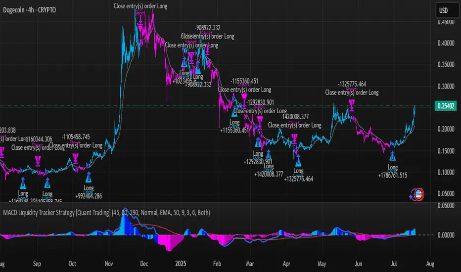
Example - DOGE Optimization (45/80/290 settings) :
• Performance : Optimized parameters yielding exceptional backtesting results with 29,800% PnL
• Why it works : DOGE's high volatility and social sentiment-driven price action benefits from heavily smoothed indicators
• Timeframes : Particularly effective on 30-minute and 4-hour charts for swing trading
• Logic : The very slow parameters filter out noise and capture only the most significant trend changes
Other Optimizable Cryptocurrencies : This parameter flexibility makes the strategy highly effective for major altcoins including SUI, SEI, LINK, Solana (SOL) , and many others. Each crypto asset can benefit from custom parameter tuning based on its unique volatility profile and trading characteristics.
Four Trading System Types
1. Normal System (Default)
Long signals : When MACD line is above the signal line
Short signals : When MACD line is below the signal line
Best for : Swing trading and capturing longer-term trends in stable markets
Logic : Traditional MACD crossover approach using the signal line
2. Fast System
Long signals : Bright Blue OR Dark Magenta (transparent) histogram colors
Short signals : Dark Blue (transparent) OR Bright Magenta histogram colors
Best for : Scalping and high-volatility markets (crypto, forex)
Logic : Leverages early momentum shifts based on histogram color changes
3. Safe System
Long signals : Only Bright Blue histogram color (strongest bullish momentum)
Short signals : All other colors (Dark Blue, Bright Magenta, Dark Magenta)
Best for : Risk-averse traders and choppy markets
Logic : Prioritizes only the strongest bullish signals while treating everything else as bearish
4. Crossover System
Long signals : MACD line crosses above signal line
Short signals : MACD line crosses below signal line
Best for : Precise timing entries with traditional MACD methodology
Logic : Pure crossover signals for more precise entry timing
Color-Coded Histogram Logic
The strategy uses four distinct colors to visualize momentum:
🔹 Bright Blue : MACD > 0 and rising (strong bullish momentum)
🔹 Dark Blue (Transparent) : MACD > 0 but falling (weakening bullish momentum)
🔹 Bright Magenta : MACD < 0 and falling (strong bearish momentum)
🔹 Dark Magenta (Transparent) : MACD < 0 but rising (weakening bearish momentum)
Trend Filter Integration
The strategy includes an advanced trend filter using 9 different moving average types:
SMA (Simple Moving Average)
EMA (Exponential Moving Average) - Default
WMA (Weighted Moving Average)
HMA (Hull Moving Average)
RMA (Running Moving Average)
LSMA (Least Squares Moving Average)
DEMA (Double Exponential Moving Average)
TEMA (Triple Exponential Moving Average)
VIDYA (Variable Index Dynamic Average)
Default Settings : 50-period EMA for trend identification
Visual Signal System
Entry Markers : Blue triangles (▲) below candles for long entries, Magenta triangles (▼) above candles for short entries
Candle Coloring : Price candles change color based on active signals (Blue = Long, Magenta = Short)
Signal Text : Optional "Long" or "Short" text inside entry triangles (toggleable)
Trend MA : Gray line plotted on main chart for trend reference
Parameter Optimization Examples
DOGE Trading Success (Optimized Parameters) :
Using 45/80/290 MACD settings with 50-period EMA trend filter has shown exceptional results on DOGE:
Performance : Backtesting results showing 29,800% PnL demonstrate the power of proper parameter optimization
Reasoning : DOGE's meme-driven volatility and social sentiment spikes create significant noise with traditional MACD settings
Solution : Very slow parameters (45/80/290) filter out social media-driven price spikes while capturing only major momentum shifts
Optimal Timeframes : 30-minute and 4-hour charts for swing trading opportunities
Result : Exceptionally clean signals with minimal false entries during DOGE's characteristic pump-and-dump cycles
Multi-Crypto Adaptability :
The same optimization principles apply to other major cryptocurrencies:
SUI : Benefits from smoothed parameters due to newer coin volatility patterns
SEI : Requires adjustment for its unique DeFi-related price movements
LINK : Oracle news events create price spikes that benefit from noise filtering
Solana (SOL) : Network congestion events and ecosystem developments need smoothed detection
General Rule : Higher volatility coins typically benefit from very slow MACD parameters (40-50 / 70-90 / 250-300 ranges)
Key Input Parameters
System Type : Choose between Fast, Normal, Safe, or Crossover (Default: Normal)
MACD Fast MA : 12 periods default (no maximum limit, consider 40-50 for crypto optimization)
MACD Slow MA : 26 periods default (no maximum limit, consider 70-90 for crypto optimization)
MACD Signal MA : 9 periods default (now properly utilized, consider 250-300 for crypto optimization)
Trend MA Type : EMA default (9 options available)
Trend MA Length : 50 periods default (no maximum limit)
Signal Display : Both, Long Only, Short Only, or None
Show Signal Text : True/False toggle for entry marker text
Trading Applications
Recommended Use Cases
Momentum Trading : Capitalize on strong directional moves using the color-coded system
Trend Following : Combine MACD signals with trend MA filter for higher probability trades
Scalping : Use "Fast" system type for quick entries in volatile markets
Swing Trading : Use "Normal" or "Safe" system types for longer-term positions
Cryptocurrency Trading : Optimize parameters for individual crypto assets (e.g., 45/80/290 for DOGE, custom settings for SUI, SEI, LINK, SOL)
Market Suitability
Volatile Markets : Forex, crypto, indices (recommend "Fast" system or smoothed parameters)
Stable Markets : Stocks, ETFs (recommend "Normal" or "Safe" system)
All Timeframes : Effective from 1-minute charts to daily charts
Crypto Optimization : Each major cryptocurrency (DOGE, SUI, SEI, LINK, SOL, etc.) can benefit from custom parameter tuning. Consider slower MACD parameters for noise reduction in volatile crypto markets
Alert System
The strategy provides comprehensive alerts for:
Entry Signals : Long and short entry triangle appearances
Exit Signals : Position exit notifications
Color Changes : Individual histogram color alerts
Trend Conditions : Price above/below trend MA alerts
Strategy Parameters
Default Settings
Initial Capital : $1,000
Position Size : 100% of equity
Commission : 0.1%
Slippage : 3 points
Date Range : January 1, 2018 to December 31, 2069
Risk Management (Optional)
Stop Loss : Disabled by default (customizable percentage-based)
Take Profit : Disabled by default (customizable percentage-based)
Short Trades : Disabled by default (can be enabled)
Important Notes and Limitations
Backtesting Considerations
Uses realistic commission (0.1%) and slippage (3 points)
Default position sizing uses 100% equity - adjust based on risk tolerance
Stop-loss and take-profit are disabled by default to show raw strategy performance
Strategy does not use lookahead bias or future data
Risk Warnings
Past performance does not guarantee future results
MACD-based strategies may produce false signals in ranging markets
Consider combining with additional confluences like support/resistance levels
Test thoroughly on demo accounts before live trading
Adjust position sizing based on your risk management requirements
Technical Limitations
Strategy does not work on non-standard chart types (Heikin Ashi, Renko, etc.)
Signals are based on close prices and may not reflect intraday price action
Multiple rapid signals in volatile conditions may result in overtrading
Credits and Attribution
This strategy is based on the original "MACD Liquidity Tracker System" indicator created by TheNeWSystemLqtyTrckr . This strategy version includes significant enhancements:
Complete strategy implementation with entry/exit logic
Addition of the "Crossover" system type
Proper implementation and utilization of the MACD signal line
Enhanced risk management features
Improved parameter flexibility with no artificial maximum limits
Additional alert systems for comprehensive trade management
The original indicator's core color logic and visual system have been preserved while expanding functionality for automated trading applications.
在腳本中搜尋"沪深主板45度上升的股票"
MTF RSI CandlesThis Pine Script indicator is designed to provide a visual representation of Relative Strength Index (RSI) values across multiple timeframes. It enhances traditional candlestick charts by color-coding candles based on RSI levels, offering a clearer picture of overbought, oversold, and sideways market conditions. Additionally, it displays a hoverable table with RSI values for multiple predefined timeframes.
Key Features
1. Candle Coloring Based on RSI Levels:
Candles are color-coded based on predefined RSI ranges for easy interpretation of market conditions.
RSI Levels:
75-100: Strongest Overbought (Green)
65-75: Stronger Overbought (Dark Green)
55-65: Overbought (Teal)
45-55: Sideways (Gray)
35-45: Oversold (Light Red)
25-35: Stronger Oversold (Dark Red)
0-25: Strongest Oversold (Bright Red)
2. Multi-Timeframe RSI Table:
Displays RSI values for the following timeframes:
1 Min, 2 Min, 3 Min, 4 Min, 5 Min
10 Min, 15 Min, 30 Min, 1 Hour, 1 Day, 1 Week
Helps traders identify RSI trends across different time horizons.
3. Hoverable RSI Values:
Displays the RSI value of any candle when hovering over it, providing additional insights for analysis.
Inputs
1. RSI Length:
Default: 14
Determines the calculation period for the RSI indicator.
2. RSI Levels:
Configurable thresholds for RSI zones:
75-100: Strongest Overbought
65-75: Stronger Overbought
55-65: Overbought
45-55: Sideways
35-45: Oversold
25-35: Stronger Oversold
0-25: Strongest Oversold
How It Works:
1. RSI Calculation:
The RSI is calculated for the current timeframe using the input RSI Length.
It is also computed for 11 additional predefined timeframes using request.security.
2. Candle Coloring:
Candles are colored based on their RSI values and the specified RSI levels.
3. Hoverable RSI Values:
Each candle displays its RSI value when hovered over, via a dynamically created label.
Multi-Timeframe Table:
A table at the bottom-left of the chart displays RSI values for all predefined timeframes, making it easy to compare trends.
Usage:
1. Trend Identification:
Use candle colors to quickly assess market conditions (overbought, oversold, or sideways).
2. Timeframe Analysis:
Compare RSI values across different timeframes to determine long-term and short-term momentum.
3. Signal Confirmation:
Combine RSI signals with other indicators or patterns for higher-confidence trades.
Best Practices
Use this indicator in conjunction with volume analysis, support/resistance levels, or trendline strategies for better results.
Customize RSI levels and timeframes based on your trading strategy or market conditions.
Limitations
RSI is a lagging indicator and may not always predict immediate market reversals.
Multi-timeframe analysis can lead to conflicting signals; consider your trading horizon.

Choppiness Index (levels)This Pine Script is a Choppiness Index Indicator with gradient visual enhancements. The Choppiness Index is a technical analysis tool that measures the "choppiness" or sideways movement of the market. It ranges from 0 to 100, where higher values indicate a more consolidated or sideways market, and lower values suggest a trending market.
Key Features:
Choppiness Index Calculation:
The script calculates the Choppiness Index based on the Average True Range (ATR) and the highest and lowest prices over a user-defined period (length).
Visual Bands:
Horizontal dashed lines are drawn at levels 55 (Upper Band), 50 (Middle Band), and 45 (Lower Band) to define key levels for interpreting the indicator.
Gradient Fills:
A blue fill is applied between the upper and lower bands (45–55) for visual clarity.
Dynamic gradients are applied to the areas:
Above the Upper Band (55–100): A green gradient fill where the color intensity increases with higher values.
Below the Lower Band (0–45): A red gradient fill where the color intensity increases with lower values.
Offset Option:
The offset input allows users to shift the Choppiness Index plot horizontally for visualization or alignment purposes.
Usage:
This indicator helps traders quickly assess market conditions:
Values above 55 indicate a choppy, non-trending market.
Values below 45 indicate a trending market.
The gradient fills make it easier to spot extreme conditions visually.
Customization:
Users can adjust:
length: The calculation period for the Choppiness Index.
offset: Horizontal shift of the Choppiness Index plot.
The gradient colors (green and red) and transparency levels are customizable in the script.
This enhanced visualization is ideal for traders who want a clear and intuitive representation of market choppiness, combined with visually striking gradient fills for quick analysis of market conditions.

G&S SMT### Description of the Pine Script
This Pine Script is designed to identify **Smart Money Technique (SMT)** setups between **Gold (GC1!)** and **Silver (SI1!) Futures** on a **15-minute timeframe**. It specifically looks for divergences between the price movements of Gold and Silver over the last 4 candles and compares it with the next candle's price movement. The script provides **Bullish** and **Bearish** signals for SMT during a specified time range of **8:45 AM EST to 10:30 AM EST**.
### Key Features of the Script:
1. **Futures Symbols**:
- The script uses **Gold Futures (GC1!)** and **Silver Futures (SI1!)** on a 15-minute timeframe to monitor their price movements.
2. **Time Range Filtering**:
- The signals are only active between **8:45 AM EST and 10:30 AM EST**, ensuring that the script only signals within the most relevant trading hours for your strategy.
3. **SMT Calculation (Last 4 Candles vs Next Candle)**:
- **Gold and Silver Price Change Calculation**: The script compares the price changes of **Gold** and **Silver** over the **last 4 candles** and then compares them with the price movement of the **next candle**:
- **Bullish SMT**: Occurs when Gold shows an increase in the last 4 candles while Silver shows a decrease, and both Gold and Silver show an increase in the next candle.
- **Bearish SMT**: Occurs when Gold shows a decrease in the last 4 candles while Silver shows an increase, and both Gold and Silver show a decrease in the next candle.
4. **Bullish and Bearish Signals**:
- **Bullish SMT Signal**: The script will plot a **green** arrow below the bar when a Bullish SMT setup is identified.
- **Bearish SMT Signal**: A **red** arrow above the bar is plotted when a Bearish SMT setup is identified.
5. **Gold and Silver Difference Plot**:
- The difference between the prices of **Gold** and **Silver** is plotted as a **blue line**, giving a visual representation of the relationship between the two assets. When the difference line moves significantly, it can indicate a potential divergence or convergence in the prices of Gold and Silver.
### Script Logic Breakdown:
1. **Price Change for Last 4 Candles**:
- The script calculates the price change for Gold and Silver from the 4th-to-last candle to the last candle.
- `gold_change_last4` and `silver_change_last4` calculate these price differences.
2. **Price Change for Next Candle**:
- It then calculates the price change from the last candle to the next candle.
- `gold_change_next` and `silver_change_next` calculate these price differences.
3. **Bullish SMT Condition**:
- If Gold increased while Silver decreased in the last 4 candles, and both Gold and Silver show an increase in the next candle, it indicates a **Bullish SMT**.
4. **Bearish SMT Condition**:
- If Gold decreased while Silver increased in the last 4 candles, and both Gold and Silver show a decrease in the next candle, it indicates a **Bearish SMT**.
5. **Time Filter**:
- Signals are only plotted when the current time is between **8:45 AM EST and 10:30 AM EST** to match your preferred trading hours.
### Visualization:
- **Bullish Signals**: Plotted as **green arrows** below the bars when a Bullish SMT setup is identified.
- **Bearish Signals**: Plotted as **red arrows** above the bars when a Bearish SMT setup is identified.
- **Gold - Silver Difference**: A **blue line** is plotted to show the price difference between Gold and Silver, helping visualize any divergence.
### How It Helps:
- **Divergence Identification**: This script highlights potential divergences between Gold and Silver Futures, which can provide insights into market sentiment and smart money movements.
- **Focus on Relevant Time Frame**: By filtering signals between 8:45 AM EST and 10:30 AM EST, you are focusing on a timeframe that can be more beneficial for trading.
- **Visual Clarity**: The arrows and the price difference line provide clear signals and a visual representation of the relationship between Gold and Silver, helping you make informed trading decisions.
This script is an automated approach to detecting **SMT setups** and helping traders recognize when Gold and Silver might be signaling a bullish or bearish move based on their divergence patterns.

ICT Setup 03 [TradingFinder] Judas Swing NY 9:30am + CHoCH/FVG🔵 Introduction
Judas Swing is an advanced trading setup designed to identify false price movements early in the trading day. This advanced trading strategy operates on the principle that major market players, or "smart money," drive price in a certain direction during the early hours to mislead smaller traders.
This deceptive movement attracts liquidity at specific levels, allowing larger players to execute primary trades in the opposite direction, ultimately causing the price to return to its true path.
The Judas Swing setup functions within two primary time frames, tailored separately for Forex and Stock markets. In the Forex market, the setup uses the 8:15 to 8:30 AM window to identify the high and low points, followed by the 8:30 to 8:45 AM frame to execute the Judas move and identify the CISD Level break, where Order Block and Fair Value Gap (FVG) zones are subsequently detected.
In the Stock market, these time frames shift to 9:15 to 9:30 AM for identifying highs and lows and 9:30 to 9:45 AM for executing the Judas move and CISD Level break.
Concepts such as Order Block and Fair Value Gap (FVG) are crucial in this setup. An Order Block represents a chart region with a high volume of buy or sell orders placed by major financial institutions, marking significant levels where price reacts.
Fair Value Gap (FVG) refers to areas where price has moved rapidly without balance between supply and demand, highlighting zones of potential price action and future liquidity.
Bullish Setup :
Bearish Setup :
🔵 How to Use
The Judas Swing setup enables traders to pinpoint entry and exit points by utilizing Order Block and FVG concepts, helping them align with liquidity-driven moves orchestrated by smart money. This setup applies two distinct time frames for Forex and Stocks to capture early deceptive movements, offering traders optimized entry or exit moments.
🟣 Bullish Setup
In the Bullish Judas Swing setup, the first step is to identify High and Low points within the initial time frame. These levels serve as key points where price may react, forming the basis for analyzing the setup and assisting traders in anticipating future market shifts.
In the second time frame, a critical stage of the bullish setup begins. During this phase, the price may create a false break or Fake Break below the low level, a deceptive move by major players to absorb liquidity. This false move often causes smaller traders to enter positions incorrectly. After this fake-out, the price reverses upward, breaking the CISD Level, a critical point in the market structure, signaling a potential bullish trend.
Upon breaking the CISD Level and reversing upward, the indicator identifies both the Order Block and Fair Value Gap (FVG). The Order Block is an area where major players typically place large buy orders, signaling potential price support. Meanwhile, the FVG marks a region of supply-demand imbalance, signaling areas where price might react.
Ultimately, after these key zones are identified, a trader may open a buy position if the price reaches one of these critical areas—Order Block or FVG—and reacts positively. Trading at these levels enhances the chance of success due to liquidity absorption and support from smart money, marking an opportune time for entering a long position.
🟣 Bearish Setup
In the Bearish Judas Swing setup, analysis begins with marking the High and Low levels in the initial time frame. These levels serve as key zones where price could react, helping to signal possible trend reversals. Identifying these levels is essential for locating significant bearish zones and positioning traders to capitalize on downward movements.
In the second time frame, the primary bearish setup unfolds. During this stage, price may exhibit a Fake Break above the high, causing a brief move upward and misleading smaller traders into incorrect positions. After this false move, the price typically returns downward, breaking the CISD Level—a crucial bearish trend indicator.
With the CISD Level broken and a bearish trend confirmed, the indicator identifies the Order Block and Fair Value Gap (FVG). The Bearish Order Block is a region where smart money places significant sell orders, prompting a negative price reaction. The FVG denotes an area of supply-demand imbalance, signifying potential selling pressure.
When the price reaches one of these critical areas—the Bearish Order Block or FVG—and reacts downward, a trader may initiate a sell position. Entering trades at these levels, due to increased selling pressure and liquidity absorption, offers traders an advantage in profiting from price declines.
🔵 Settings
Market : The indicator allows users to choose between Forex and Stocks, automatically adjusting the time frames for the "Opening Range" and "Trading Permit" accordingly: Forex: 8:15–8:30 AM for identifying High and Low points, and 8:30–8:45 AM for capturing the Judas move and CISD Level break. Stocks: 9:15–9:30 AM for identifying High and Low points, and 9:30–9:45 AM for executing the Judas move and CISD Level break.
Refine Order Block : Enables finer adjustments to Order Block levels for more accurate price responses.
Mitigation Level OB : Allows users to set specific reaction points within an Order Block, including: Proximal: Closest level to the current price. 50% OB: Midpoint of the Order Block. Distal: Farthest level from the current price.
FVG Filter : The Judas Swing indicator includes a filter for Fair Value Gap (FVG), allowing different filtering based on FVG width: FVG Filter Type: Can be set to "Very Aggressive," "Aggressive," "Defensive," or "Very Defensive." Higher defensiveness narrows the FVG width, focusing on narrower gaps.
Mitigation Level FVG : Like the Order Block, you can set price reaction levels for FVG with options such as Proximal, 50% OB, and Distal.
CISD : The Bar Back Check option enables traders to specify the number of past candles checked for identifying the CISD Level, enhancing CISD Level accuracy on the chart.
🔵 Conclusion
The Judas Swing indicator helps traders spot reliable trading opportunities by detecting false price movements and key levels such as Order Block and FVG. With a focus on early market movements, this tool allows traders to align with major market participants, selecting entry and exit points with greater precision, thereby reducing trading risks.
Its extensive customization options enable adjustments for various market types and trading conditions, giving traders the flexibility to optimize their strategies. Based on ICT techniques and liquidity analysis, this indicator can be highly effective for those seeking precision in their entry points.
Overall, Judas Swing empowers traders to capitalize on significant market movements by leveraging price volatility. Offering precise and dependable signals, this tool presents an excellent opportunity for enhancing trading accuracy and improving performance

Dema Percentile Standard DeviationDema Percentile Standard Deviation
The Dema Percentile Standard Deviation indicator is a robust tool designed to identify and follow trends in financial markets.
How it works?
This code is straightforward and simple:
The price is smoothed using a DEMA (Double Exponential Moving Average).
Percentiles are then calculated on that DEMA.
When the closing price is below the lower percentile, it signals a potential short.
When the closing price is above the upper percentile and the Standard Deviation of the lower percentile, it signals a potential long.
Settings
Dema/Percentile/SD/EMA Length's: Defines the period over which calculations are made.
Dema Source: The source of the price data used in calculations.
Percentiles: Selects the type of percentile used in calculations (options include 60/40, 60/45, 55/40, 55/45). In these settings, 60 and 55 determine percentile for long signals, while 45 and 40 determine percentile for short signals.
Features
Fully Customizable
Fully Customizable: Customize colors to display for long/short signals.
Display Options: Choose to show long/short signals as a background color, as a line on price action, or as trend momentum in a separate window.
EMA for Confluence: An EMA can be used for early entries/exits for added signal confirmation, but it may introduce noise—use with caution!
Built-in Alerts.
Indicator on Diffrent Assets
INDEX:BTCUSD 1D Chart (6 high 56 27 60/45 14)
CRYPTO:SOLUSD 1D Chart (24 open 31 20 60/40 14)
CRYPTO:RUNEUSD 1D Chart (10 close 56 14 60/40 14)
Remember no indicator would on all assets with default setting so FAFO with setting to get your desired signal.
Hayden's Advanced Relative Strength Index (RSI)Preface: I'm just the bartender serving today's freshly blended concoction; I'd like to send a massive THANK YOU to @iFuSiiOnzZ, @Koalafied_3, @LonesomeTheBlue, @LazyBear, @dgtrd and the rest of the PineWizards for the locally-sourced ingredients. I am simply a code editor, not a code author. The book that inspired this indicator is a free download, plus all of the pieces I used were free code from the PineWizards; my hope is that any additional useful development of The Complete RSI trading system also is offered open-source to the community for collaboration.
Features: Fixed & Custom price targeting. Triple trend state detection. Advanced data ticker. Candles, bars, or line RSI . Stochastic of over 20 indicators for adjustable entry/exit signals. Customizable trader watermark. Trend lines for spotting wedges , triangles, pennants , etc. Divergences for spotting potential reversals and Momentum Discrepancy Reversal Point opportunities. RSI percent change and price pivot labels. Gradient bar coloring on-chart.
‼ IMPORTANT: Hover over labels for additional information. Google & read John Hayden's "The Complete RSI" pdf book for comprehensive instructions before attempting to trade with this indicator. Always keep an eye on higher/stronger timeframes.
⚠ DISCLAIMER: DYOR. Not financial advice. Not a trading system. I am not affiliated with TradingView or John Hayden; this is my own personally PineScripted presentation of a suitable RSI to use when trading according to Hayden's rules.
About the Editor: I am a former-FINRA Registered Representative, inventor/patent-holder, and self-taught PineScripter. I mostly code on a v3 Pinescript level so expect heavy scripts that could use some shortening with modern conventions.
Hayden's RSI Rules:
📈 An Uptrend is indicated when:
1. RSI is in the 80 to 40 range
2. The chart shows simple bearish divergence
3. The chart shows Hidden bullish divergence
4. The chart shows Momentum Discrepancy Reversal Up
5. Upside targets being hit
6. 9-bar simple MA is greater than the 45-bar EMA on RSI
7. Counter-trend declines do not exceed 50% of the previous rally
🔮 An Uptrend is in danger when:
1. Longer timeframe fading rally
2. a) Multiple long-term bearish divergences. b) Upside targets not being hit.
3. 9-bar simple MA is less than the 45-bar EMA on RSI
4. Hidden bearish divergence, or simple bullish divergence
5. Deep counter-trend retracements greater than 50%
📉 A Downtrend is indicated when:
1. RSI is in the 60 to 20 range
2. The chart shows simple bullish divergences.
3. The chart shows Hidden bearish divergence
4. The chart shows Momentum Discrepancy Reversal Down
5. Downside targets being hit
6. 9-bar simple MA is less than the 45-bar EMA on RSI
7. Counter-trend rallies do not exceed 50% of the previous decline
🔮 A Downtrend is in danger when:
1. Longer timeframe fading decline
2. a) Multiple long-term bullish divergences. b) Downside targets not being hit.
3. 9-bar simple MA is greater than the 45-bar EMA on RSI
4. Hidden bullish divergence , or simple bearish divergence
5. Steep counter-trend retracements greater than 50%
Gann Circle Intraday LevelsThis indicator is an intraday version of Gann Circle Swing Levels indicator. It further divides the Gann Circle into the Eighths in order to generate intraday Levels.
Introduction
This indicator is based on W. D. Gann's Square of 9 Chart and can be interpreted as the Gann Circle / Gann Wheel / 360 Degree Circle Chart or Square of the Circle Chart for intraday usage.
Spiral arrangement of numbers on the Square of 9 chart creates a very unique square root relationship amongst the numbers on the chart. If you take any number on the Square of 9 chart, take the square root of the number, then add 2 to the root and re-square it, resulting in one full 360 degree cycle (i.e. a 360 degree Circle) out from the center of the chart.
For example,
the square root of 121 = 11,
11 + 2 = 13,
and the square of 13 = 169
The number 169 is one full 360 degree cycle out (with reference to 121) from the center of the Square of 9 chart. If we further divide the circle in eight equal parts of 45 degree each, following intermediate resistance levels (ascending) would be generated:
127 (45 degree)
133 (90 degree)
139 (135 degree)
145 (180 degree)
151 (225 degree)
157 (270 degree)
163 (315 degree)
Similarly, if you take any number on the Square of 9 chart, take the square root of the number, then subtract 2 from the root and re-square it, resulting in one full 360 degree inward rotation towards the center of the chart.
For example,
the square root of 565 = 23.77,
23.77 - 2 = 21.77,
and the square of 21.77 = 473.93 (approximately equal to 474, which is directly below 565 on the Square of 9 chart)
The number 474 is one full 360 degree inward rotation (with reference to 565) towards the center of the chart. If we further divide the circle in eight equal parts of 45 degree each, following intermediate support levels (descending) would be generated:
553 (45 degree)
541 (90 degree)
529 (135 degree)
518 (180 degree)
507 (225 degree)
496 (270 degree)
485 (315 degree)
How to Use this Indicator ?
This indicator is designed to generate Gann Circle Intraday Levels based on HIGH and LOW of the opening bar for the day. You may use the bar interval (1 minute, 3 minutes, 5 minutes, 15 minutes etc.) which is suitable for the underlying instrument. Support and resistance lines for the day would be generated only after confirmation of the opening bar of the day.
Input :
Number of Gann Levels (Number of Gann Levels to be projected)
Color codes for the Support and Resistance Levels
Output :
Gann Support or Resistance Levels:
HIGH and LOW of the Opening bar for the day (dashed BLUE lines)
Support levels calculated with reference to the HIGH of the opening bar
Resistance levels calculated with reference to the LOW of the opening bar
CHOP Zone Entry Strategy + DMI/PSAR ExitThis is a Strategy with associated visual indicators and Long/Short and Reverse/Close Position Alerts for the Choppiness Index (CHOP) . It is used to determine if the market is choppy (trading sideways) or not choppy (trading within a trend in either direction). CHOP is not directional, so a DMI script was ported into this strategy to allow for trend confirmation and direction determination; it consists of an Average Directional Index (ADX) , Plus Directional Indicator (+DI) and Minus Directional Indicator (-DI) . In addition, a Parabolic SAR is also included to act as a trailing stop during any strong trends.
Development Notes
---------------------------
This indicator, and most of the descriptions below, were derived largely from the TradingView reference manual. Feedback and suggestions for improvement are more than welcome, as well are recommended Input settings and best practices for use.
www.tradingview.com
www.tradingview.com
www.tradingview.com
Recommend using the below DMI and PSAR indicators in conjunction with this script to fully visualize and understand how entry and exit conditions are chosen. Variable inputs should correlate between the scripts for uniformity and visual compatibility.
THANKS to LazyBear and his Momentum Squeeze script for helping me quickly develop a momentum state model for coloring the Chop line by trend.
Strategy Description
---------------------------
CHOP produces values that determine whether the market is choppy or trending . The closer the value is to 100 , the higher the choppiness levels , while the closer it is to 0 , the stronger the market is trending . Territories for both levels, and their associated upper and lower thresholds, are popularly defined using the Fibonacci Retracements, 61.8 and 38.2.
Basic Use
---------------------------
CHOP is often used to confirm the market condition to help you stay out of sideways markets and only enter when there is movement or imminent explosions. When readings are above the upper threshold, continued sideways movement may be expected, while readings below the lower threshold are typically indicative of a continuing trend. It is also used to anticipate upcoming trendiness changes, with the general belief that extended periods of consolidation (sideways movement) are followed by extended periods of strong, trending, directional movement, and vice versa.
One limitation in this index is that you must be cautious in deciding whether the range or trend will likely continue, or if it will reverse.
Confidence in price action and trend is higher when two or more indicators are in agreement -- while this strategy combines CHOP with both DMI and PSAR, we would still recommend pairing with other indicators to determine entry or exit trade opportunities.
Recommend also choosing 'Once Per Bar Close' when creating alerts.
Inputs
---------------------------
Strategy Direction - an option to only trade Short, Long, Both, or only in the direction of the Trend (Follow Trend is the Default).
Sensitivity - an incremental variable to test whether the past n candles are in the same trend state before triggering a delayed long or short alert (1 is the Default). Can help filter out noise and reduces active alerts.
Show Chop Index - two visual styles are provided for user preference, a visible Chop line with a background overlay, or a compact column and label only view.
Chop Lookback Period - the time period to be used in calculating CHOP (14 is the Default).
Chop Offset - changing this number will move the CHOP either forwards or backwards relative to the current market (0 is the Default).
Smooth Chop Line and Length - if enabled, the entered time period will be used in calculating a smooth average of the index (Enabled and 4 are the Defaults).
Color Line to Trend Direction - toggles whether the index line is colored to visually depict the current trend direction (Enabled is the Default).
Color Background - toggles the visibility of a background color based on the index state (Enabled is the Default).
Enable DMI Option - if enabled, then entry will be confirmed by and dependent on the ADX Key Level, with any close or reversal confirmed by both ADX and +/-DI to determine whether there is a strong trend present or not (Enabled is the Default).
ADX Smoothing - the time period to be used in calculating the ADX which has a smoothing component (14 is the Default).
DI Length - the time period to be used in calculating the DI (14 is the Default).
ADX Key Level - any trade with the ADX above the key level is a strong indicator that it is trending (23 to 25 is the suggested setting).
Enable PSAR Option - enables trailing stop loss orders (Enabled is the Default).
PSAR Start - the starting value for the Acceleration Force (0.015 is our chosen Default, 0.02 is more common).
PSAR Increment - the increment in which the Acceleration Force will move (0.001 is our chosen Default, 0.02 is more common).
PSAR Max Value - the maximum value of the Acceleration Factor (0.2 is the Default).
Color Candles Option - an option to transpose the CHOP condition levels to the main candle bars. Note that the outer red and green border will still be distinguished by whether each individual candle is bearish or bullish during the specified timeframe.
Note too that if both DMI and PSAR are deselected, then close determinations will default to a CHOP reversal strategy (e.g., close long when below 38.2 and close short when above 61.8). Though if either DMI or PSAR are enabled, then the CHOP reversal for close determination will automatically be disabled.
Indicator Visuals
---------------------------
For the candle colors, black indicates tight chop (45 to 55), yellow is loose chop (38.2 to 45 and 55 to 61.8), dark purple is trending down (< 38.2), and dark blue is trending up (> 61.8).
The background color has additional shades to differentiate a wider range of more levels…
• < 30 is dark purple
• 30 to 38.2 is purple
• 38.2 to 45 is light purple
• 45 to 55 is black
• 55 to 61.8 is light blue
• 61.8 to 70 is blue
• > 70 is dark blue
Long, Short, Close, and Reverse labels are plotted on the Chop line, which itself can be colored based on the trend. The chop line can also be hidden for a clean and compact, columnar view, which is my preferred option (see example image below).
Visual cues are intended to improve analysis and decrease interpretation time during trading, as well as to aid in understanding the purpose of this strategy and how its inclusion can benefit a comprehensive trading plan.
DMI and Trend Strength
---------------------------
To analyze trend strength, the focus should be on the ADX line and not the +DI or -DI lines. An ADX reading above 25 indicates a strong trend , while a reading below 20 indicates a weak or non-existent trend . A reading between those two values would be considered indeterminable. Though what is truly a strong trend or a weak trend depends on the financial instrument being examined; historical analysis can assist in determining appropriate values.
DMI exits trade when ADX is below the user selected key level (e.g., default is 25) and when the +/- DI lines cross (e.g., -DI > +DI exits long position and +DI > -DI exits short position).
PSAR and Trailing Stop
---------------------------
PSAR is a time and price based indicator that excels at measuring direction and duration, though not the actual strength of a trend, which is why we use this in conjunction with DMI. It is also included in this script as a trailing stop option to maximize gains during strong trends and to mitigate any false ADX strengthening signals.
This creates a parabola that is located below the candle during a Bullish trend and above during a Bearish trend. A buy or reversal is signaled when the price crosses above or below the Parabolic SAR.
Long/Short Entry
---------------------------
1. CHOP must be over 61.8 (long) or under 38.2 (short).
2. If DMI is enabled, then the ADX signal line must be above the user selected Key Level (default is 25).
3. If Sensitivity is selected, then that past candle must meet the criteria in step 1, as well as all the intermediate candles in between.
4. If "Follow Trend" is selected and PSAR is enabled, then a long position can only open when the momentum and PSAR are in an uptrend, or short when both are in a downtrend, to include all intermediate candles if the Sensitivity option is set on a past candle.
Close/Reverse
---------------------------
1. If DMI is enabled, then a close flag will be raised when the ADX signal drops below the Key Level (of 25), and -DI crosses over +DI (if long), or +DI crosses over -DI (if short).
2. If PSAR is enabled, then a close flag will be raised when the current trend state is opposite the last state.
3. If both DMI and PSAR are disabled, then a close flag will be raised if the Chop line drops under 38.2 (if long) or goes over 61.8 (if short).
4. If a Long or Short Entry is triggered on the same candle as any of the above close flags, then the position will be reversed, else the position will be closed.
Strategy Alerts
---------------------------
1. Long Entry
2. Short Entry
3. Reverse
4. Close
The provided backtest result is based on a position sizing of 10% equity with 100k initial capital. When testing SPX, disabling the DMI performed the best, but EURUSD performed poorly without it enabled, and TSLA had a small reduction in net profit. Timeframe likewise differed between commodities with TSLA performing best at 30M, SPX at 15M, and EURUSD at 4H. I do not plan on using this as a standalone strategy, but I also was expecting better results with the inclusion of EMI and PSAR to compliment the CHOP. Key elements of this script will likely be included in future, more holistic strategies.
Disclaimer
---------------------------
Past performance may not be indicative of future results. Due to various factors, including changing market conditions, the strategy may no longer perform as well as in historical backtesting. This post and the script are not intended to provide any financial advice. Trade at your own risk.
No known repainting, though there may be if an offset is introduced in the Inputs. I did my best not to code any other variables that repaint, but cannot fully attest to this fact.
Ruckard TradingLatinoThis strategy tries to mimic TradingLatino strategy.
The current implementation is beta.
Si hablas castellano o espanyol por favor consulta MENSAJE EN CASTELLANO más abajo.
It's aimed at BTCUSDT pair and 4h timeframe.
STRATEGY DEFAULT SETTINGS EXPLANATION
max_bars_back=5000 : This is a random number of bars so that the strategy test lasts for one or two years
calc_on_order_fills=false : To wait for the 4h closing is too much. Try to check if it's worth entering a position after closing one. I finally decided not to recheck if it's worth entering after an order is closed. So it is false.
calc_on_every_tick=false
pyramiding=0 : We only want one entry allowed in the same direction. And we don't want the order to scale by error.
initial_capital=1000 : These are 1000 USDT. By using 1% maximum loss per trade and 7% as a default stop loss by using 1000 USDT at 12000 USDT per BTC price you would entry with around 142 USDT which are converted into: 0.010 BTC . The maximum number of decimal for contracts on this BTCUSDT market is 3 decimals. E.g. the minimum might be: 0.001 BTC . So, this minimal 1000 amount ensures us not to entry with less than 0.001 entries which might have happened when using 100 USDT as an initial capital.
slippage=1 : Binance BTCUSDT mintick is: 0.01. Binance slippage: 0.1 % (Let's assume). TV has an integer slippage. It does not have a percentage based slippage. If we assume a 1000 initial capital, the recommended equity is 142 which at 11996 USDT per BTC price means: 0.011 BTC. The 0.1% slippage of: 0.011 BTC would be: 0.000011 . This is way smaller than the mintick. So our slippage is going to be 1. E.g. 1 (slippage) * 0.01 (mintick)
commission_type=strategy.commission.percent and commission_value=0.1 : According to: binance . com / en / fee / schedule in VIP 0 level both maker and taker fees are: 0.1 %.
BACKGROUND
Jaime Merino is a well known Youtuber focused on crypto trading
His channel TradingLatino
features monday to friday videos where he explains his strategy.
JAIME MERINO STANCE ON BOTS
Jaime Merino stance on bots (taken from memory out of a 2020 June video from him):
'~
You know. They can program you a bot and it might work.
But, there are some special situations that the bot would not be able to handle.
And, I, as a human, I would handle it. And the bot wouldn't do it.
~'
My long term target with this strategy script is add as many
special situations as I can to the script
so that it can match Jaime Merino behaviour even in non normal circumstances.
My alternate target is learn Pine script
and enjoy programming with it.
WARNING
This script might be bigger than other TradingView scripts.
However, please, do not be confused because the current status is beta.
This script has not been tested with real money.
This is NOT an official strategy from Jaime Merino.
This is NOT an official strategy from TradingLatino . net .
HOW IT WORKS
It basically uses ADX slope and LazyBear's Squeeze Momentum Indicator
to make its buy and sell decisions.
Fast paced EMA being bigger than slow paced EMA
(on higher timeframe) advices going long.
Fast paced EMA being smaller than slow paced EMA
(on higher timeframe) advices going short.
It finally add many substrats that TradingLatino uses.
SETTINGS
__ SETTINGS - Basics
____ SETTINGS - Basics - ADX
(ADX) Smoothing {14}
(ADX) DI Length {14}
(ADX) key level {23}
____ SETTINGS - Basics - LazyBear Squeeze Momentum
(SQZMOM) BB Length {20}
(SQZMOM) BB MultFactor {2.0}
(SQZMOM) KC Length {20}
(SQZMOM) KC MultFactor {1.5}
(SQZMOM) Use TrueRange (KC) {True}
____ SETTINGS - Basics - EMAs
(EMAS) EMA10 - Length {10}
(EMAS) EMA10 - Source {close}
(EMAS) EMA55 - Length {55}
(EMAS) EMA55 - Source {close}
____ SETTINGS - Volume Profile
Lowest and highest VPoC from last three days
is used to know if an entry has a support
VPVR of last 100 4h bars
is also taken into account
(VP) Use number of bars (not VP timeframe): Uses 'Number of bars {100}' setting instead of 'Volume Profile timeframe' setting for calculating session VPoC
(VP) Show tick difference from current price {False}: BETA . Might be useful for actions some day.
(VP) Number of bars {100}: If 'Use number of bars (not VP timeframe)' is turned on this setting is used to calculate session VPoC.
(VP) Volume Profile timeframe {1 day}: If 'Use number of bars (not VP timeframe)' is turned off this setting is used to calculate session VPoC.
(VP) Row width multiplier {0.6}: Adjust how the extra Volume Profile bars are shown in the chart.
(VP) Resistances prices number of decimal digits : Round Volume Profile bars label numbers so that they don't have so many decimals.
(VP) Number of bars for bottom VPOC {18}: 18 bars equals 3 days in suggested timeframe of 4 hours. It's used to calculate lowest session VPoC from previous three days. It's also used as a top VPOC for sells.
(VP) Ignore VPOC bottom advice on long {False}: If turned on it ignores bottom VPOC (or top VPOC on sells) when evaluating if a buy entry is worth it.
(VP) Number of bars for VPVR VPOC {100}: Number of bars to calculate the VPVR VPoC. We use 100 as Jaime once used. When the price bounces back to the EMA55 it might just bounce to this VPVR VPoC if its price it's lower than the EMA55 (Sells have inverse algorithm).
____ SETTINGS - ADX Slope
ADX Slope
help us to understand if ADX
has a positive slope, negative slope
or it is rather still.
(ADXSLOPE) ADX cut {23}: If ADX value is greater than this cut (23) then ADX has strength
(ADXSLOPE) ADX minimum steepness entry {45}: ADX slope needs to be 45 degrees to be considered as a positive one.
(ADXSLOPE) ADX minimum steepness exit {45}: ADX slope needs to be -45 degrees to be considered as a negative one.
(ADXSLOPE) ADX steepness periods {3}: In order to avoid false detection the slope is calculated along 3 periods.
____ SETTINGS - Next to EMA55
(NEXTEMA55) EMA10 to EMA55 bounce back percentage {80}: EMA10 might bounce back to EMA55 or maybe to 80% of its complete way to EMA55
(NEXTEMA55) Next to EMA55 percentage {15}: How much next to the EMA55 you need to be to consider it's going to bounce back upwards again.
____ SETTINGS - Stop Loss and Take Profit
You can set a default stop loss or a default take profit.
(STOPTAKE) Stop Loss % {7.0}
(STOPTAKE) Take Profit % {2.0}
____ SETTINGS - Trailing Take Profit
You can customize the default trailing take profit values
(TRAILING) Trailing Take Profit (%) {1.0}: Trailing take profit offset in percentage
(TRAILING) Trailing Take Profit Trigger (%) {2.0}: When 2.0% of benefit is reached then activate the trailing take profit.
____ SETTINGS - MAIN TURN ON/OFF OPTIONS
(EMAS) Ignore advice based on emas {false}.
(EMAS) Ignore advice based on emas (On closing long signal) {False}: Ignore advice based on emas but only when deciding to close a buy entry.
(SQZMOM) Ignore advice based on SQZMOM {false}: Ignores advice based on SQZMOM indicator.
(ADXSLOPE) Ignore advice based on ADX positive slope {false}
(ADXSLOPE) Ignore advice based on ADX cut (23) {true}
(STOPTAKE) Take Profit? {false}: Enables simple Take Profit.
(STOPTAKE) Stop Loss? {True}: Enables simple Stop Loss.
(TRAILING) Enable Trailing Take Profit (%) {True}: Enables Trailing Take Profit.
____ SETTINGS - Strategy mode
(STRAT) Type Strategy: 'Long and Short', 'Long Only' or 'Short Only'. Default: 'Long and Short'.
____ SETTINGS - Risk Management
(RISKM) Risk Management Type: 'Safe', 'Somewhat safe compound' or 'Unsafe compound'. ' Safe ': Calculations are always done with the initial capital (1000) in mind. The maximum losses per trade/day/week/month are taken into account. ' Somewhat safe compound ': Calculations are done with initial capital (1000) or a higher capital if it increases. The maximum losses per trade/day/week/month are taken into account. ' Unsafe compound ': In each order all the current capital is gambled and only the default stop loss per order is taken into account. That means that the maximum losses per trade/day/week/month are not taken into account. Default : 'Somewhat safe compound'.
(RISKM) Maximum loss per trade % {1.0}.
(RISKM) Maximum loss per day % {6.0}.
(RISKM) Maximum loss per week % {8.0}.
(RISKM) Maximum loss per month % {10.0}.
____ SETTINGS - Decimals
(DECIMAL) Maximum number of decimal for contracts {3}: How small (3 decimals means 0.001) an entry position might be in your exchange.
EXTRA 1 - PRICE IS IN RANGE indicator
(PRANGE) Print price is in range {False}: Enable a bottom label that indicates if the price is in range or not.
(PRANGE) Price range periods {5}: How many previous periods are used to calculate the medians
(PRANGE) Price range maximum desviation (%) {0.6} ( > 0 ): Maximum positive desviation for range detection
(PRANGE) Price range minimum desviation (%) {0.6} ( > 0 ): Mininum negative desviation for range detection
EXTRA 2 - SQUEEZE MOMENTUM Desviation indicator
(SQZDIVER) Show degrees {False}: Show degrees of each Squeeze Momentum Divergence lines to the x-axis.
(SQZDIVER) Show desviation labels {False}: Whether to show or not desviation labels for the Squeeze Momentum Divergences.
(SQZDIVER) Show desviation lines {False}: Whether to show or not desviation lines for the Squeeze Momentum Divergences.
EXTRA 3 - VOLUME PROFILE indicator
WARNING: This indicator works not on current bar but on previous bar. So in the worst case it might be VP from 4 hours ago. Don't worry, inside the strategy calculus the correct values are used. It's just that I cannot show the most recent one in the chart.
(VP) Print recent profile {False}: Show Volume Profile indicator
(VP) Avoid label price overlaps {False}: Avoid label prices to overlap on the chart.
EXTRA 4 - ZIGNALY SUPPORT
(ZIG) Zignaly Alert Type {Email}: 'Email', 'Webhook'. ' Email ': Prepare alert_message variable content to be compatible with zignaly expected email content format. ' Webhook ': Prepare alert_message variable content to be compatible with zignaly expected json content format.
EXTRA 5 - DEBUG
(DEBUG) Enable debug on order comments {False}: If set to true it prepares the order message to match the alert_message variable. It makes easier to debug what would have been sent by email or webhook on each of the times an order is triggered.
HOW TO USE THIS STRATEGY
BOT MODE: This is the default setting.
PROPER VOLUME PROFILE VIEWING: Click on this strategy settings. Properties tab. Make sure Recalculate 'each time the order was run' is turned off.
NEWBIE USER: (Check PROPER VOLUME PROFILE VIEWING above!) You might want to turn on the 'Print recent profile {False}' setting. Alternatively you can use my alternate realtime study: 'Resistances and supports based on simplified Volume Profile' but, be aware, it might consume one indicator.
ADVANCED USER 1: Turn on the 'Print price is in range {False}' setting and help us to debug this subindicator. Also help us to figure out how to include this value in the strategy.
ADVANCED USER 2: Turn on the all the (SQZDIVER) settings and help us to figure out how to include this value in the strategy.
ADVANCED USER 3: (Check PROPER VOLUME PROFILE VIEWING above!) Turn on the 'Print recent profile {False}' setting and report any problem with it.
JAIME MERINO: Just use the indicator as it comes by default. It should only show BUY signals, SELL signals and their associated closing signals. From time to time you might want to check 'ADVANCED USER 2' instructions to check that there's actually a divergence. Check also 'ADVANCED USER 1' instructions for your amusement.
EXTRA ADVICE
It's advised that you use this strategy in addition to these two other indicators:
* Squeeze Momentum Indicator
* ADX
so that your chart matches as close as possible to TradingLatino chart.
ZIGNALY INTEGRATION
This strategy supports Zignaly email integration by default. It also supports Zignaly Webhook integration.
ZIGNALY INTEGRATION - Email integration example
What you would write in your alert message:
||{{strategy.order.alert_message}}||key=MYSECRETKEY||
ZIGNALY INTEGRATION - Webhook integration example
What you would write in your alert message:
{ {{strategy.order.alert_message}} , "key" : "MYSECRETKEY" }
CREDITS
I have reused and adapted some code from
'Directional Movement Index + ADX & Keylevel Support' study
which it's from TradingView console user.
I have reused and adapted some code from
'3ema' study
which it's from TradingView hunganhnguyen1193 user.
I have reused and adapted some code from
'Squeeze Momentum Indicator ' study
which it's from TradingView LazyBear user.
I have reused and adapted some code from
'Strategy Tester EMA-SMA-RSI-MACD' study
which it's from TradingView fikira user.
I have reused and adapted some code from
'Support Resistance MTF' study
which it's from TradingView LonesomeTheBlue user.
I have reused and adapted some code from
'TF Segmented Linear Regression' study
which it's from TradingView alexgrover user.
I have reused and adapted some code from
"Poor man's volume profile" study
which it's from TradingView IldarAkhmetgaleev user.
FEEDBACK
Please check the strategy source code for more detailed information
where, among others, I explain all of the substrats
and if they are implemented or not.
Q1. Did I understand wrong any of the Jaime substrats (which I have implemented)?
Q2. The strategy yields quite profit when we should long (EMA10 from 1d timeframe is higher than EMA55 from 1d timeframe.
Why the strategy yields much less profit when we should short (EMA10 from 1d timeframe is lower than EMA55 from 1d timeframe)?
Any idea if you need to do something else rather than just reverse what Jaime does when longing?
FREQUENTLY ASKED QUESTIONS
FAQ1. Why are you giving this strategy for free?
TradingLatino and his fellow enthusiasts taught me this strategy. Now I'm giving back to them.
FAQ2. Seriously! Why are you giving this strategy for free?
I'm confident his strategy might be improved a lot. By keeping it to myself I would avoid other people contributions to improve it.
Now that everyone can contribute this is a win-win.
FAQ3. How can I connect this strategy to my Exchange account?
It seems that you can attach alerts to strategies.
You might want to combine it with a paying account which enable Webhook URLs to work.
I don't know how all of this works right now so I cannot give you advice on it.
You will have to do your own research on this subject. But, be careful. Automating trades, if not done properly,
might end on you automating losses.
FAQ4. I have just found that this strategy by default gives more than 3.97% of 'maximum series of losses'. That's unacceptable according to my risk management policy.
You might want to reduce default stop loss setting from 7% to something like 5% till you are ok with the 'maximum series of losses'.
FAQ5. Where can I learn more about your work on this strategy?
Check the source code. You might find unused strategies. Either because there's not a substantial increases on earnings. Or maybe because they have not been implemented yet.
FAQ6. How much leverage is applied in this strategy?
No leverage.
FAQ7. Any difference with original Jaime Merino strategy?
Most of the times Jaime defines an stop loss at the price entry. That's not the case here. The default stop loss is 7% (but, don't be confused it only means losing 1% of your investment thanks to risk management). There's also a trailing take profit that triggers at 2% profit with a 1% trailing.
FAQ8. Why this strategy return is so small?
The strategy should be improved a lot. And, well, backtesting in this platform is not guaranteed to return theoric results comparable to real-life returns. That's why I'm personally forward testing this strategy to verify it.
MENSAJE EN CASTELLANO
En primer lugar se agradece feedback para mejorar la estrategia.
Si eres un usuario avanzado y quieres colaborar en mejorar el script no dudes en comentar abajo.
Ten en cuenta que aunque toda esta descripción tenga que estar en inglés no es obligatorio que el comentario esté en inglés.
CHISTE - CASTELLANO
¡Pero Jaime!
¡400.000!
¡Tu da mun!
Traders Dynamic Index(RSI) w/ Bull&Bear Control ZonesMomentum (RSI) is one of the most commonly used indicators for trading, but the vast majority of traders who use it, simply apply it as an oscillator to measure overbought and oversold conditions. However, momentum is much more complex than that and using a basic RSI fails to highlight these complexities.
What this highlights are some of the areas/zones that many people may not even know about or are unaware what the RSI can actually reveal about a particular trend.
What this indicator is showing:
Fast moving RSI (Green) - 1 period
Slow moving RSI (Red) - 9 period
Bollinger Bands
Relative Strength: 1 - 100
Bearish Control Zone: 30(Below) - 45
Bullish Control Zone: 60 - 70 (Above)
How this identifies trends:
Bear Market(Bearish Control Zone):
-Support: 20(Below) - 30
-Resistance: 55 - 65
-Momentum will test resistance but will fail to hold support at 50
Bull Market(Bullish Control Zone):
-Support: 45 - 50
-Resistance: 80 - 90(Above)
-Momentum will test support but will not continue past the 45 support
How this identifies reversals:
If a market is bullish, but loses support at 45 and tests 30, it has begun reversal. If a market is bearish, but breaks 60 and tests 70, it has begun reversal.
-A bull market reversal is confirmed if it finds resistance at 60 after testing bearish support
-A bear market reversal is confirmed if it finds support at 50 after testing bullish resistance
Slow & Fast RSI w/ Boll Bands:
-The Slow and Fast RSI crossovers will act as Intermediate trends within the Macro trend - Fast crosses slow, bullish. Slow cross fast, bearish.
-Use in confluence with the Macro trend.
-While under Bearish Control, the Slow RSI will act as resistance for the Fast RSI.
-While under Bullish Control, the Slow RSI will act as support for the Fast RSI.
-The two will have an impulsive crossover when the Macro trend reverses.
-The Bollinger Bands will act as a volatility gauge for potential approaching tests of Support & Resistances. (Expansions & Contractions)
This is an analog of TDIGM (GoldMinds)
-Added Bullish/Bearish Control Zones.
-Changed Fast RSI to Green and Slow RSI to Red.

Percentage OscillatorUsing momentum calculations on multiple time frames and adding everything together into 4 separate directions:
1- green: the strength and momentum in +45 to +90 degrees angle
2- blue: the strength and momentum in 0 to +45 degrees angle
3- orange: the strength and momentum in 0 to -45 degrees angle
4- red: the strength and momentum in -45 to -90 degrees angle
Single parameter to control the size of the largest moving window.
Uptrend is green with orange corrections
Downtrend is red with blue corrections
When downtrend turns into uptrend, blue becomes green
When uptrend turns into downtrend, orange becomes red
The natural cycle of the market is RED->BLUE->GREEN->ORANGE and so on, you will see the cycle repeats itself 3 times before a break up\down. The strength of the movement depends on the height and width of all the waves that created the 3 cycle movement (reminds Elliot in an oscillatory representation)
The script is provided as is, there are no trading strategies implied or recommended.
Feel free to PM with questions

Kelly Position Size CalculatorThis position sizing calculator implements the Kelly Criterion, developed by John L. Kelly Jr. at Bell Laboratories in 1956, to determine mathematically optimal position sizes for maximizing long-term wealth growth. Unlike arbitrary position sizing methods, this tool provides a scientifically solution based on your strategy's actual performance statistics and incorporates modern refinements from over six decades of academic research.
The Kelly Criterion addresses a fundamental question in capital allocation: "What fraction of capital should be allocated to each opportunity to maximize growth while avoiding ruin?" This question has profound implications for financial markets, where traders and investors constantly face decisions about optimal capital allocation (Van Tharp, 2007).
Theoretical Foundation
The Kelly Criterion for binary outcomes is expressed as f* = (bp - q) / b, where f* represents the optimal fraction of capital to allocate, b denotes the risk-reward ratio, p indicates the probability of success, and q represents the probability of loss (Kelly, 1956). This formula maximizes the expected logarithm of wealth, ensuring maximum long-term growth rate while avoiding the risk of ruin.
The mathematical elegance of Kelly's approach lies in its derivation from information theory. Kelly's original work was motivated by Claude Shannon's information theory (Shannon, 1948), recognizing that maximizing the logarithm of wealth is equivalent to maximizing the rate of information transmission. This connection between information theory and wealth accumulation provides a deep theoretical foundation for optimal position sizing.
The logarithmic utility function underlying the Kelly Criterion naturally embodies several desirable properties for capital management. It exhibits decreasing marginal utility, penalizes large losses more severely than it rewards equivalent gains, and focuses on geometric rather than arithmetic mean returns, which is appropriate for compounding scenarios (Thorp, 2006).
Scientific Implementation
This calculator extends beyond basic Kelly implementation by incorporating state of the art refinements from academic research:
Parameter Uncertainty Adjustment: Following Michaud (1989), the implementation applies Bayesian shrinkage to account for parameter estimation error inherent in small sample sizes. The adjustment formula f_adjusted = f_kelly × confidence_factor + f_conservative × (1 - confidence_factor) addresses the overconfidence bias documented by Baker and McHale (2012), where the confidence factor increases with sample size and the conservative estimate equals 0.25 (quarter Kelly).
Sample Size Confidence: The reliability of Kelly calculations depends critically on sample size. Research by Browne and Whitt (1996) provides theoretical guidance on minimum sample requirements, suggesting that at least 30 independent observations are necessary for meaningful parameter estimates, with 100 or more trades providing reliable estimates for most trading strategies.
Universal Asset Compatibility: The calculator employs intelligent asset detection using TradingView's built-in symbol information, automatically adapting calculations for different asset classes without manual configuration.
ASSET SPECIFIC IMPLEMENTATION
Equity Markets: For stocks and ETFs, position sizing follows the calculation Shares = floor(Kelly Fraction × Account Size / Share Price). This straightforward approach reflects whole share constraints while accommodating fractional share trading capabilities.
Foreign Exchange Markets: Forex markets require lot-based calculations following Lot Size = Kelly Fraction × Account Size / (100,000 × Base Currency Value). The calculator automatically handles major currency pairs with appropriate pip value calculations, following industry standards described by Archer (2010).
Futures Markets: Futures position sizing accounts for leverage and margin requirements through Contracts = floor(Kelly Fraction × Account Size / Margin Requirement). The calculator estimates margin requirements as a percentage of contract notional value, with specific adjustments for micro-futures contracts that have smaller sizes and reduced margin requirements (Kaufman, 2013).
Index and Commodity Markets: These markets combine characteristics of both equity and futures markets. The calculator automatically detects whether instruments are cash-settled or futures-based, applying appropriate sizing methodologies with correct point value calculations.
Risk Management Integration
The calculator integrates sophisticated risk assessment through two primary modes:
Stop Loss Integration: When fixed stop-loss levels are defined, risk calculation follows Risk per Trade = Position Size × Stop Loss Distance. This ensures that the Kelly fraction accounts for actual risk exposure rather than theoretical maximum loss, with stop-loss distance measured in appropriate units for each asset class.
Strategy Drawdown Assessment: For discretionary exit strategies, risk estimation uses maximum historical drawdown through Risk per Trade = Position Value × (Maximum Drawdown / 100). This approach assumes that individual trade losses will not exceed the strategy's historical maximum drawdown, providing a reasonable estimate for strategies with well-defined risk characteristics.
Fractional Kelly Approaches
Pure Kelly sizing can produce substantial volatility, leading many practitioners to adopt fractional Kelly approaches. MacLean, Sanegre, Zhao, and Ziemba (2004) analyze the trade-offs between growth rate and volatility, demonstrating that half-Kelly typically reduces volatility by approximately 75% while sacrificing only 25% of the growth rate.
The calculator provides three primary Kelly modes to accommodate different risk preferences and experience levels. Full Kelly maximizes growth rate while accepting higher volatility, making it suitable for experienced practitioners with strong risk tolerance and robust capital bases. Half Kelly offers a balanced approach popular among professional traders, providing optimal risk-return balance by reducing volatility significantly while maintaining substantial growth potential. Quarter Kelly implements a conservative approach with low volatility, recommended for risk-averse traders or those new to Kelly methodology who prefer gradual introduction to optimal position sizing principles.
Empirical Validation and Performance
Extensive academic research supports the theoretical advantages of Kelly sizing. Hakansson and Ziemba (1995) provide a comprehensive review of Kelly applications in finance, documenting superior long-term performance across various market conditions and asset classes. Estrada (2008) analyzes Kelly performance in international equity markets, finding that Kelly-based strategies consistently outperform fixed position sizing approaches over extended periods across 19 developed markets over a 30-year period.
Several prominent investment firms have successfully implemented Kelly-based position sizing. Pabrai (2007) documents the application of Kelly principles at Berkshire Hathaway, noting Warren Buffett's concentrated portfolio approach aligns closely with Kelly optimal sizing for high-conviction investments. Quantitative hedge funds, including Renaissance Technologies and AQR, have incorporated Kelly-based risk management into their systematic trading strategies.
Practical Implementation Guidelines
Successful Kelly implementation requires systematic application with attention to several critical factors:
Parameter Estimation: Accurate parameter estimation represents the greatest challenge in practical Kelly implementation. Brown (1976) notes that small errors in probability estimates can lead to significant deviations from optimal performance. The calculator addresses this through Bayesian adjustments and confidence measures.
Sample Size Requirements: Users should begin with conservative fractional Kelly approaches until achieving sufficient historical data. Strategies with fewer than 30 trades may produce unreliable Kelly estimates, regardless of adjustments. Full confidence typically requires 100 or more independent trade observations.
Market Regime Considerations: Parameters that accurately describe historical performance may not reflect future market conditions. Ziemba (2003) recommends regular parameter updates and conservative adjustments when market conditions change significantly.
Professional Features and Customization
The calculator provides comprehensive customization options for professional applications:
Multiple Color Schemes: Eight professional color themes (Gold, EdgeTools, Behavioral, Quant, Ocean, Fire, Matrix, Arctic) with dark and light theme compatibility ensure optimal visibility across different trading environments.
Flexible Display Options: Adjustable table size and position accommodate various chart layouts and user preferences, while maintaining analytical depth and clarity.
Comprehensive Results: The results table presents essential information including asset specifications, strategy statistics, Kelly calculations, sample confidence measures, position values, risk assessments, and final position sizes in appropriate units for each asset class.
Limitations and Considerations
Like any analytical tool, the Kelly Criterion has important limitations that users must understand:
Stationarity Assumption: The Kelly Criterion assumes that historical strategy statistics represent future performance characteristics. Non-stationary market conditions may invalidate this assumption, as noted by Lo and MacKinlay (1999).
Independence Requirement: Each trade should be independent to avoid correlation effects. Many trading strategies exhibit serial correlation in returns, which can affect optimal position sizing and may require adjustments for portfolio applications.
Parameter Sensitivity: Kelly calculations are sensitive to parameter accuracy. Regular calibration and conservative approaches are essential when parameter uncertainty is high.
Transaction Costs: The implementation incorporates user-defined transaction costs but assumes these remain constant across different position sizes and market conditions, following Ziemba (2003).
Advanced Applications and Extensions
Multi-Asset Portfolio Considerations: While this calculator optimizes individual position sizes, portfolio-level applications require additional considerations for correlation effects and aggregate risk management. Simplified portfolio approaches include treating positions independently with correlation adjustments.
Behavioral Factors: Behavioral finance research reveals systematic biases that can interfere with Kelly implementation. Kahneman and Tversky (1979) document loss aversion, overconfidence, and other cognitive biases that lead traders to deviate from optimal strategies. Successful implementation requires disciplined adherence to calculated recommendations.
Time-Varying Parameters: Advanced implementations may incorporate time-varying parameter models that adjust Kelly recommendations based on changing market conditions, though these require sophisticated econometric techniques and substantial computational resources.
Comprehensive Usage Instructions and Practical Examples
Implementation begins with loading the calculator on your desired trading instrument's chart. The system automatically detects asset type across stocks, forex, futures, and cryptocurrency markets while extracting current price information. Navigation to the indicator settings allows input of your specific strategy parameters.
Strategy statistics configuration requires careful attention to several key metrics. The win rate should be calculated from your backtest results using the formula of winning trades divided by total trades multiplied by 100. Average win represents the sum of all profitable trades divided by the number of winning trades, while average loss calculates the sum of all losing trades divided by the number of losing trades, entered as a positive number. The total historical trades parameter requires the complete number of trades in your backtest, with a minimum of 30 trades recommended for basic functionality and 100 or more trades optimal for statistical reliability. Account size should reflect your available trading capital, specifically the risk capital allocated for trading rather than total net worth.
Risk management configuration adapts to your specific trading approach. The stop loss setting should be enabled if you employ fixed stop-loss exits, with the stop loss distance specified in appropriate units depending on the asset class. For stocks, this distance is measured in dollars, for forex in pips, and for futures in ticks. When stop losses are not used, the maximum strategy drawdown percentage from your backtest provides the risk assessment baseline. Kelly mode selection offers three primary approaches: Full Kelly for aggressive growth with higher volatility suitable for experienced practitioners, Half Kelly for balanced risk-return optimization popular among professional traders, and Quarter Kelly for conservative approaches with reduced volatility.
Display customization ensures optimal integration with your trading environment. Eight professional color themes provide optimization for different chart backgrounds and personal preferences. Table position selection allows optimal placement within your chart layout, while table size adjustment ensures readability across different screen resolutions and viewing preferences.
Detailed Practical Examples
Example 1: SPY Swing Trading Strategy
Consider a professionally developed swing trading strategy for SPY (S&P 500 ETF) with backtesting results spanning 166 total trades. The strategy achieved 110 winning trades, representing a 66.3% win rate, with an average winning trade of $2,200 and average losing trade of $862. The maximum drawdown reached 31.4% during the testing period, and the available trading capital amounts to $25,000. This strategy employs discretionary exits without fixed stop losses.
Implementation requires loading the calculator on the SPY daily chart and configuring the parameters accordingly. The win rate input receives 66.3, while average win and loss inputs receive 2200 and 862 respectively. Total historical trades input requires 166, with account size set to 25000. The stop loss function remains disabled due to the discretionary exit approach, with maximum strategy drawdown set to 31.4%. Half Kelly mode provides the optimal balance between growth and risk management for this application.
The calculator generates several key outputs for this scenario. The risk-reward ratio calculates automatically to 2.55, while the Kelly fraction reaches approximately 53% before scientific adjustments. Sample confidence achieves 100% given the 166 trades providing high statistical confidence. The recommended position settles at approximately 27% after Half Kelly and Bayesian adjustment factors. Position value reaches approximately $6,750, translating to 16 shares at a $420 SPY price. Risk per trade amounts to approximately $2,110, representing 31.4% of position value, with expected value per trade reaching approximately $1,466. This recommendation represents the mathematically optimal balance between growth potential and risk management for this specific strategy profile.
Example 2: EURUSD Day Trading with Stop Losses
A high-frequency EURUSD day trading strategy demonstrates different parameter requirements compared to swing trading approaches. This strategy encompasses 89 total trades with a 58% win rate, generating an average winning trade of $180 and average losing trade of $95. The maximum drawdown reached 12% during testing, with available capital of $10,000. The strategy employs fixed stop losses at 25 pips and take profit targets at 45 pips, providing clear risk-reward parameters.
Implementation begins with loading the calculator on the EURUSD 1-hour chart for appropriate timeframe alignment. Parameter configuration includes win rate at 58, average win at 180, and average loss at 95. Total historical trades input receives 89, with account size set to 10000. The stop loss function is enabled with distance set to 25 pips, reflecting the fixed exit strategy. Quarter Kelly mode provides conservative positioning due to the smaller sample size compared to the previous example.
Results demonstrate the impact of smaller sample sizes on Kelly calculations. The risk-reward ratio calculates to 1.89, while the Kelly fraction reaches approximately 32% before adjustments. Sample confidence achieves 89%, providing moderate statistical confidence given the 89 trades. The recommended position settles at approximately 7% after Quarter Kelly application and Bayesian shrinkage adjustment for the smaller sample. Position value amounts to approximately $700, translating to 0.07 standard lots. Risk per trade reaches approximately $175, calculated as 25 pips multiplied by lot size and pip value, with expected value per trade at approximately $49. This conservative position sizing reflects the smaller sample size, with position sizes expected to increase as trade count surpasses 100 and statistical confidence improves.
Example 3: ES1! Futures Systematic Strategy
Systematic futures trading presents unique considerations for Kelly criterion application, as demonstrated by an E-mini S&P 500 futures strategy encompassing 234 total trades. This systematic approach achieved a 45% win rate with an average winning trade of $1,850 and average losing trade of $720. The maximum drawdown reached 18% during the testing period, with available capital of $50,000. The strategy employs 15-tick stop losses with contract specifications of $50 per tick, providing precise risk control mechanisms.
Implementation involves loading the calculator on the ES1! 15-minute chart to align with the systematic trading timeframe. Parameter configuration includes win rate at 45, average win at 1850, and average loss at 720. Total historical trades receives 234, providing robust statistical foundation, with account size set to 50000. The stop loss function is enabled with distance set to 15 ticks, reflecting the systematic exit methodology. Half Kelly mode balances growth potential with appropriate risk management for futures trading.
Results illustrate how favorable risk-reward ratios can support meaningful position sizing despite lower win rates. The risk-reward ratio calculates to 2.57, while the Kelly fraction reaches approximately 16%, lower than previous examples due to the sub-50% win rate. Sample confidence achieves 100% given the 234 trades providing high statistical confidence. The recommended position settles at approximately 8% after Half Kelly adjustment. Estimated margin per contract amounts to approximately $2,500, resulting in a single contract allocation. Position value reaches approximately $2,500, with risk per trade at $750, calculated as 15 ticks multiplied by $50 per tick. Expected value per trade amounts to approximately $508. Despite the lower win rate, the favorable risk-reward ratio supports meaningful position sizing, with single contract allocation reflecting appropriate leverage management for futures trading.
Example 4: MES1! Micro-Futures for Smaller Accounts
Micro-futures contracts provide enhanced accessibility for smaller trading accounts while maintaining identical strategy characteristics. Using the same systematic strategy statistics from the previous example but with available capital of $15,000 and micro-futures specifications of $5 per tick with reduced margin requirements, the implementation demonstrates improved position sizing granularity.
Kelly calculations remain identical to the full-sized contract example, maintaining the same risk-reward dynamics and statistical foundations. However, estimated margin per contract reduces to approximately $250 for micro-contracts, enabling allocation of 4-5 micro-contracts. Position value reaches approximately $1,200, while risk per trade calculates to $75, derived from 15 ticks multiplied by $5 per tick. This granularity advantage provides better position size precision for smaller accounts, enabling more accurate Kelly implementation without requiring large capital commitments.
Example 5: Bitcoin Swing Trading
Cryptocurrency markets present unique challenges requiring modified Kelly application approaches. A Bitcoin swing trading strategy on BTCUSD encompasses 67 total trades with a 71% win rate, generating average winning trades of $3,200 and average losing trades of $1,400. Maximum drawdown reached 28% during testing, with available capital of $30,000. The strategy employs technical analysis for exits without fixed stop losses, relying on price action and momentum indicators.
Implementation requires conservative approaches due to cryptocurrency volatility characteristics. Quarter Kelly mode is recommended despite the high win rate to account for crypto market unpredictability. Expected position sizing remains reduced due to the limited sample size of 67 trades, requiring additional caution until statistical confidence improves. Regular parameter updates are strongly recommended due to cryptocurrency market evolution and changing volatility patterns that can significantly impact strategy performance characteristics.
Advanced Usage Scenarios
Portfolio position sizing requires sophisticated consideration when running multiple strategies simultaneously. Each strategy should have its Kelly fraction calculated independently to maintain mathematical integrity. However, correlation adjustments become necessary when strategies exhibit related performance patterns. Moderately correlated strategies should receive individual position size reductions of 10-20% to account for overlapping risk exposure. Aggregate portfolio risk monitoring ensures total exposure remains within acceptable limits across all active strategies. Professional practitioners often consider using lower fractional Kelly approaches, such as Quarter Kelly, when running multiple strategies simultaneously to provide additional safety margins.
Parameter sensitivity analysis forms a critical component of professional Kelly implementation. Regular validation procedures should include monthly parameter updates using rolling 100-trade windows to capture evolving market conditions while maintaining statistical relevance. Sensitivity testing involves varying win rates by ±5% and average win/loss ratios by ±10% to assess recommendation stability under different parameter assumptions. Out-of-sample validation reserves 20% of historical data for parameter verification, ensuring that optimization doesn't create curve-fitted results. Regime change detection monitors actual performance against expected metrics, triggering parameter reassessment when significant deviations occur.
Risk management integration requires professional overlay considerations beyond pure Kelly calculations. Daily loss limits should cease trading when daily losses exceed twice the calculated risk per trade, preventing emotional decision-making during adverse periods. Maximum position limits should never exceed 25% of account value in any single position regardless of Kelly recommendations, maintaining diversification principles. Correlation monitoring reduces position sizes when holding multiple correlated positions that move together during market stress. Volatility adjustments consider reducing position sizes during periods of elevated VIX above 25 for equity strategies, adapting to changing market conditions.
Troubleshooting and Optimization
Professional implementation often encounters specific challenges requiring systematic troubleshooting approaches. Zero position size displays typically result from insufficient capital for minimum position sizes, negative expected values, or extremely conservative Kelly calculations. Solutions include increasing account size, verifying strategy statistics for accuracy, considering Quarter Kelly mode for conservative approaches, or reassessing overall strategy viability when fundamental issues exist.
Extremely high Kelly fractions exceeding 50% usually indicate underlying problems with parameter estimation. Common causes include unrealistic win rates, inflated risk-reward ratios, or curve-fitted backtest results that don't reflect genuine trading conditions. Solutions require verifying backtest methodology, including all transaction costs in calculations, testing strategies on out-of-sample data, and using conservative fractional Kelly approaches until parameter reliability improves.
Low sample confidence below 50% reflects insufficient historical trades for reliable parameter estimation. This situation demands gathering additional trading data, using Quarter Kelly approaches until reaching 100 or more trades, applying extra conservatism in position sizing, and considering paper trading to build statistical foundations without capital risk.
Inconsistent results across similar strategies often stem from parameter estimation differences, market regime changes, or strategy degradation over time. Professional solutions include standardizing backtest methodology across all strategies, updating parameters regularly to reflect current conditions, and monitoring live performance against expectations to identify deteriorating strategies.
Position sizes that appear inappropriately large or small require careful validation against traditional risk management principles. Professional standards recommend never risking more than 2-3% per trade regardless of Kelly calculations. Calibration should begin with Quarter Kelly approaches, gradually increasing as comfort and confidence develop. Most institutional traders utilize 25-50% of full Kelly recommendations to balance growth with prudent risk management.
Market condition adjustments require dynamic approaches to Kelly implementation. Trending markets may support full Kelly recommendations when directional momentum provides favorable conditions. Ranging or volatile markets typically warrant reducing to Half or Quarter Kelly to account for increased uncertainty. High correlation periods demand reducing individual position sizes when multiple positions move together, concentrating risk exposure. News and event periods often justify temporary position size reductions during high-impact releases that can create unpredictable market movements.
Performance monitoring requires systematic protocols to ensure Kelly implementation remains effective over time. Weekly reviews should compare actual versus expected win rates and average win/loss ratios to identify parameter drift or strategy degradation. Position size efficiency and execution quality monitoring ensures that calculated recommendations translate effectively into actual trading results. Tracking correlation between calculated and realized risk helps identify discrepancies between theoretical and practical risk exposure.
Monthly calibration provides more comprehensive parameter assessment using the most recent 100 trades to maintain statistical relevance while capturing current market conditions. Kelly mode appropriateness requires reassessment based on recent market volatility and performance characteristics, potentially shifting between Full, Half, and Quarter Kelly approaches as conditions change. Transaction cost evaluation ensures that commission structures, spreads, and slippage estimates remain accurate and current.
Quarterly strategic reviews encompass comprehensive strategy performance analysis comparing long-term results against expectations and identifying trends in effectiveness. Market regime assessment evaluates parameter stability across different market conditions, determining whether strategy characteristics remain consistent or require fundamental adjustments. Strategic modifications to position sizing methodology may become necessary as markets evolve or trading approaches mature, ensuring that Kelly implementation continues supporting optimal capital allocation objectives.
Professional Applications
This calculator serves diverse professional applications across the financial industry. Quantitative hedge funds utilize the implementation for systematic position sizing within algorithmic trading frameworks, where mathematical precision and consistent application prove essential for institutional capital management. Professional discretionary traders benefit from optimized position management that removes emotional bias while maintaining flexibility for market-specific adjustments. Portfolio managers employ the calculator for developing risk-adjusted allocation strategies that enhance returns while maintaining prudent risk controls across diverse asset classes and investment strategies.
Individual traders seeking mathematical optimization of capital allocation find the calculator provides institutional-grade methodology previously available only to professional money managers. The Kelly Criterion establishes theoretical foundation for optimal capital allocation across both single strategies and multiple trading systems, offering significant advantages over arbitrary position sizing methods that rely on intuition or fixed percentage approaches. Professional implementation ensures consistent application of mathematically sound principles while adapting to changing market conditions and strategy performance characteristics.
Conclusion
The Kelly Criterion represents one of the few mathematically optimal solutions to fundamental investment problems. When properly understood and carefully implemented, it provides significant competitive advantage in financial markets. This calculator implements modern refinements to Kelly's original formula while maintaining accessibility for practical trading applications.
Success with Kelly requires ongoing learning, systematic application, and continuous refinement based on market feedback and evolving research. Users who master Kelly principles and implement them systematically can expect superior risk-adjusted returns and more consistent capital growth over extended periods.
The extensive academic literature provides rich resources for deeper study, while practical experience builds the intuition necessary for effective implementation. Regular parameter updates, conservative approaches with limited data, and disciplined adherence to calculated recommendations are essential for optimal results.
References
Archer, M. D. (2010). Getting Started in Currency Trading: Winning in Today's Forex Market (3rd ed.). John Wiley & Sons.
Baker, R. D., & McHale, I. G. (2012). An empirical Bayes approach to optimising betting strategies. Journal of the Royal Statistical Society: Series D (The Statistician), 61(1), 75-92.
Breiman, L. (1961). Optimal gambling systems for favorable games. In J. Neyman (Ed.), Proceedings of the Fourth Berkeley Symposium on Mathematical Statistics and Probability (pp. 65-78). University of California Press.
Brown, D. B. (1976). Optimal portfolio growth: Logarithmic utility and the Kelly criterion. In W. T. Ziemba & R. G. Vickson (Eds.), Stochastic Optimization Models in Finance (pp. 1-23). Academic Press.
Browne, S., & Whitt, W. (1996). Portfolio choice and the Bayesian Kelly criterion. Advances in Applied Probability, 28(4), 1145-1176.
Estrada, J. (2008). Geometric mean maximization: An overlooked portfolio approach? The Journal of Investing, 17(4), 134-147.
Hakansson, N. H., & Ziemba, W. T. (1995). Capital growth theory. In R. A. Jarrow, V. Maksimovic, & W. T. Ziemba (Eds.), Handbooks in Operations Research and Management Science (Vol. 9, pp. 65-86). Elsevier.
Kahneman, D., & Tversky, A. (1979). Prospect theory: An analysis of decision under risk. Econometrica, 47(2), 263-291.
Kaufman, P. J. (2013). Trading Systems and Methods (5th ed.). John Wiley & Sons.
Kelly Jr, J. L. (1956). A new interpretation of information rate. Bell System Technical Journal, 35(4), 917-926.
Lo, A. W., & MacKinlay, A. C. (1999). A Non-Random Walk Down Wall Street. Princeton University Press.
MacLean, L. C., Sanegre, E. O., Zhao, Y., & Ziemba, W. T. (2004). Capital growth with security. Journal of Economic Dynamics and Control, 28(4), 937-954.
MacLean, L. C., Thorp, E. O., & Ziemba, W. T. (2011). The Kelly Capital Growth Investment Criterion: Theory and Practice. World Scientific.
Michaud, R. O. (1989). The Markowitz optimization enigma: Is 'optimized' optimal? Financial Analysts Journal, 45(1), 31-42.
Pabrai, M. (2007). The Dhandho Investor: The Low-Risk Value Method to High Returns. John Wiley & Sons.
Shannon, C. E. (1948). A mathematical theory of communication. Bell System Technical Journal, 27(3), 379-423.
Tharp, V. K. (2007). Trade Your Way to Financial Freedom (2nd ed.). McGraw-Hill.
Thorp, E. O. (2006). The Kelly criterion in blackjack sports betting, and the stock market. In L. C. MacLean, E. O. Thorp, & W. T. Ziemba (Eds.), The Kelly Capital Growth Investment Criterion: Theory and Practice (pp. 789-832). World Scientific.
Van Tharp, K. (2007). Trade Your Way to Financial Freedom (2nd ed.). McGraw-Hill Education.
Vince, R. (1992). The Mathematics of Money Management: Risk Analysis Techniques for Traders. John Wiley & Sons.
Vince, R., & Zhu, H. (2015). Optimal betting under parameter uncertainty. Journal of Statistical Planning and Inference, 161, 19-31.
Ziemba, W. T. (2003). The Stochastic Programming Approach to Asset, Liability, and Wealth Management. The Research Foundation of AIMR.
Further Reading
For comprehensive understanding of Kelly Criterion applications and advanced implementations:
MacLean, L. C., Thorp, E. O., & Ziemba, W. T. (2011). The Kelly Capital Growth Investment Criterion: Theory and Practice. World Scientific.
Vince, R. (1992). The Mathematics of Money Management: Risk Analysis Techniques for Traders. John Wiley & Sons.
Thorp, E. O. (2017). A Man for All Markets: From Las Vegas to Wall Street. Random House.
Cover, T. M., & Thomas, J. A. (2006). Elements of Information Theory (2nd ed.). John Wiley & Sons.
Ziemba, W. T., & Vickson, R. G. (Eds.). (2006). Stochastic Optimization Models in Finance. World Scientific.

TimezoneFormatIANAUTCLibrary "TimezoneFormatIANAUTC"
Provides either the full IANA timezone identifier or the corresponding UTC offset for TradingView’s built-in variables and functions.
tz(_tzname, _format)
Parameters:
_tzname (string) : "London", "New York", "Istanbul", "+1:00", "-03:00" etc.
_format (string) : "IANA" or "UTC"
Returns: "Europe/London", "America/New York", "UTC+1:00"
Example Code
import ARrowofTime/TimezoneFormatIANAUTC/1 as libtz
sesTZInput = input.string(defval = "Singapore", title = "Timezone")
example1 = libtz.tz("London", "IANA") // Return Europe/London
example2 = libtz.tz("London", "UTC") // Return UTC+1:00
example3 = libtz.tz("UTC+5", "IANA") // Return UTC+5:00
example4 = libtz.tz("UTC+4:30", "UTC") // Return UTC+4:30
example5 = libtz.tz(sesTZInput, "IANA") // Return Asia/Singapore
example6 = libtz.tz(sesTZInput, "UTC") // Return UTC+8:00
sesTime1 = time("","1300-1700", example1) // returns the UNIX time of the current bar in session time or na
sesTime2 = time("","1300-1700", example2) // returns the UNIX time of the current bar in session time or na
sesTime3 = time("","1300-1700", example3) // returns the UNIX time of the current bar in session time or na
sesTime4 = time("","1300-1700", example4) // returns the UNIX time of the current bar in session time or na
sesTime5 = time("","1300-1700", example5) // returns the UNIX time of the current bar in session time or na
sesTime6 = time("","1300-1700", example6) // returns the UNIX time of the current bar in session time or na
Parameter Format Guide
This section explains how to properly format the parameters for the tz(_tzname, _format) function.
_tzname (string) must be either;
A valid timezone name exactly as it appears in the chart’s lower-right corner (e.g. New York, London).
A valid UTC offset in ±H:MM or ±HH:MM format. Hours: 0–14 (zero-padded or not, e.g. +1:30, +01:30, -0:00). Minutes: Must be 00, 15, 30, or 45
examples;
"New York" → ✅ Valid chart label
"London" → ✅ Valid chart label
"Berlin" → ✅ Valid chart label
"America/New York" → ❌ Invalid chart label. (Use "New York" instead)
"+1:30" → ✅ Valid offset with single-digit hour
"+01:30" → ✅ Valid offset with zero-padded hour
"-05:00" → ✅ Valid negative offset
"-0:00" → ✅ Valid zero offset
"+1:1" → ❌ Invalid (minute must be 00, 15, 30, or 45)
"+2:50" → ❌ Invalid (minute must be 00, 15, 30, or 45)
"+15:00" → ❌ Invalid (hour must be 14 or below)
_tztype (string) must be either;
"IANA" → returns full IANA timezone identifier (e.g. "Europe/London"). When a time function call uses an IANA time zone identifier for its timezone argument, its calculations adjust automatically for historical and future changes to the specified region’s observed time, such as daylight saving time (DST) and updates to time zone boundaries, instead of using a fixed offset from UTC.
"UTC" → returns UTC offset string (e.g. "UTC+01:00")

Quantum Reversal# 🧠 Quantum Reversal
## **Quantitative Mean Reversion Framework**
This algorithmic trading system employs **statistical mean reversion theory** combined with **adaptive volatility modeling** to capitalize on Bitcoin's inherent price oscillations around its statistical mean. The strategy integrates multiple technical indicators through a **multi-layered signal processing architecture**.
---
## ⚡ **Core Technical Architecture**
### 📊 **Statistical Foundation**
- **Bollinger Band Mean Reversion Model**: Utilizes 20-period moving average with 2.2 standard deviation bands for volatility-adjusted entry signals
- **Adaptive Volatility Threshold**: Dynamic standard deviation multiplier accounts for Bitcoin's heteroscedastic volatility patterns
- **Price Action Confluence**: Entry triggered when price breaches lower volatility band, indicating statistical oversold conditions
### 🔬 **Momentum Analysis Layer**
- **RSI Oscillator Integration**: 14-period Relative Strength Index with modified oversold threshold at 45
- **Signal Smoothing Algorithm**: 5-period simple moving average applied to RSI reduces noise and false signals
- **Momentum Divergence Detection**: Captures mean reversion opportunities when momentum indicators show oversold readings
### ⚙️ **Entry Logic Architecture**
```
Entry Condition = (Price ≤ Lower_BB) OR (Smoothed_RSI < 45)
```
- **Dual-Condition Framework**: Either statistical price deviation OR momentum oversold condition triggers entry
- **Boolean Logic Gate**: OR-based entry system increases signal frequency while maintaining statistical validity
- **Position Sizing**: Fixed 10% equity allocation per trade for consistent risk exposure
### 🎯 **Exit Strategy Optimization**
- **Profit-Lock Mechanism**: Positions only closed when showing positive unrealized P&L
- **Trend Continuation Logic**: Allows winning trades to run until momentum exhaustion
- **Dynamic Exit Timing**: No fixed profit targets - exits based on profitability state rather than arbitrary levels
---
## 📈 **Statistical Properties**
### **Risk Management Framework**
- **Long-Only Exposure**: Eliminates short-squeeze risk inherent in cryptocurrency markets
- **Mean Reversion Bias**: Exploits Bitcoin's tendency to revert to statistical mean after extreme moves
- **Position Management**: Single position limit prevents over-leveraging
### **Signal Processing Characteristics**
- **Noise Reduction**: SMA smoothing on RSI eliminates high-frequency oscillations
- **Volatility Adaptation**: Bollinger Bands automatically adjust to changing market volatility
- **Multi-Timeframe Coherence**: Indicators operate on consistent timeframe for signal alignment
---
## 🔧 **Parameter Configuration**
| Technical Parameter | Value | Statistical Significance |
|-------------------|-------|-------------------------|
| Bollinger Period | 20 | Standard statistical lookback for volatility calculation |
| Std Dev Multiplier | 2.2 | Optimized for Bitcoin's volatility distribution (95.4% confidence interval) |
| RSI Period | 14 | Traditional momentum oscillator period |
| RSI Threshold | 45 | Modified oversold level accounting for Bitcoin's momentum characteristics |
| Smoothing Period | 5 | Noise reduction filter for momentum signals |
---
## 📊 **Algorithmic Advantages**
✅ **Statistical Edge**: Exploits documented mean reversion tendency in Bitcoin markets
✅ **Volatility Adaptation**: Dynamic bands adjust to changing market conditions
✅ **Signal Confluence**: Multiple indicator confirmation reduces false positives
✅ **Momentum Integration**: RSI smoothing improves signal quality and timing
✅ **Risk-Controlled Exposure**: Systematic position sizing and long-only bias
---
## 🔬 **Mathematical Foundation**
The strategy leverages **Bollinger Band theory** (developed by John Bollinger) which assumes that prices tend to revert to the mean after extreme deviations. The RSI component adds **momentum confirmation** to the statistical price deviation signal.
**Statistical Basis:**
- Mean reversion follows the principle that extreme price deviations from the moving average are temporary
- The 2.2 standard deviation multiplier captures approximately 97.2% of price movements under normal distribution
- RSI momentum smoothing reduces noise inherent in oscillator calculations
---
## ⚠️ **Risk Considerations**
This algorithm is designed for traders with understanding of **quantitative finance principles** and **cryptocurrency market dynamics**. The strategy assumes mean-reverting behavior which may not persist during trending market phases. Proper risk management and position sizing are essential.
---
## 🎯 **Implementation Notes**
- **Market Regime Awareness**: Most effective in ranging/consolidating markets
- **Volatility Sensitivity**: Performance may vary during extreme volatility events
- **Backtesting Recommended**: Historical performance analysis advised before live implementation
- **Capital Allocation**: 10% per trade sizing assumes diversified portfolio approach
---
**Engineered for quantitative traders seeking systematic mean reversion exposure in Bitcoin markets through statistically-grounded technical analysis.**
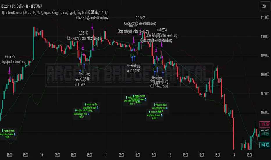
NY Opening Range Breakout - MA StopCore Concept
This strategy trades breakouts from the New York opening range (9:30-9:45 AM NY time) on intraday timeframes, designed for scalping and day trading.
Setup Requirements
Timeframe: Works on any timeframe under 15 minutes (1m, 2m, 3m, 5m, 10m)
Session: New York market hours
Range Period: 9:30-9:45 AM NY time (15-minute opening range)
Entry Rules
Long Entries:
Wait for a candle to close above the opening range high
Enter long on the next candle (before 12:00 PM NY time)
Must be above moving average if using MA-based take profit
Short Entries:
Wait for a candle to close below the opening range low
Enter short on the next candle (before 12:00 PM NY time)
Must be below moving average if using MA-based take profit
Risk Management
Stop Loss:
Long trades: Opening range low
Short trades: Opening range high
Take Profit Options:
Fixed Risk Reward: 1.5x the range size (customizable ratio)
Moving Average: Exit when price crosses back through MA
Both: Whichever comes first
Key Features
Trade Direction Options:
Long Only
Short Only
Both directions
Moving Average Filter:
Prevents entries that would immediately hit stop loss
Uses EMA/SMA/WMA/VWMA with customizable length
Acts as dynamic support/resistance
Time Restrictions:
No entries after 12:00 PM NY time (customizable cutoff)
One trade per direction per day
Daily reset of all variables
Visual Elements
Red/green lines showing opening range
Purple line for moving average
Entry and breakout signals with shapes
Take profit and stop loss levels plotted
Information table with current status
Strategy Logic Flow
Morning: Capture 9:30-9:45 range high/low
Wait: Monitor for breakout (previous candle close outside range)
Filter: Check MA condition if using MA-based exits
Enter: Trade on next candle after breakout
Manage: Exit at fixed TP, MA cross, or stop loss
Reset: Start fresh next trading day
This is a momentum-based breakout strategy that capitalizes on early market volatility while using the opening range as natural support/resistance levels.
Multi-TF Support LevelsThe Multi-TF Support Levels indicator identifies and displays key support levels based on swing lows across three user-selected timeframes.
How it works:
Input Parameters:
Lookback Period (100) — historical depth to search for swing lows.
Timeframe 1-3 (15, 45, 240) — three timeframes (e.g., 15min, 45min, 4hr).
Logic:
For each timeframe, a swing low is detected: the lowest price within the lookback period that is also lower than the two preceding candles.
Support levels update dynamically when new swing lows are formed.
The most recent levels are plotted as horizontal cross marks (blue, red, green for each timeframe).
Purpose: Visualize significant support zones from multiple timeframes to identify confluent areas for trading decisions.
Индикатор Multi-TF Support Levels (Мультитаймфреймовые уровни поддержки) определяет и отображает ключевые уровни поддержки на основе минимумов свингов (swing lows) на трёх выбранных таймфреймах.
Как работает:
Входные параметры:
Lookback Period (100) — глубина анализа для поиска минимумов.
Timeframe 1-3 (15, 45, 240) — три таймфрейма (например, 15 минут, 45 минут, 4 часа).
Логика:
Для каждого таймфрейма определяется свинг-минимум: цена, которая является самой низкой за период lookback и ниже двух предыдущих свечей.
Уровни поддержки обновляются при появлении новых свинг-минимумов.
Последние актуальные уровни отображаются на графике в виде горизонтальных линий-крестиков (синий, красный, зелёный для каждого таймфрейма).
Цель: Визуализировать значимые уровни поддержки с разных таймфреймов для поиска зон "конфлюэнса".
NIFTY BANKNIFTY MIDCAP SENSEX FINNIFTY LEVELS)this indicator uses Gann's methods which are based on the idea that markets move in predictable geometric patterns and are influenced by time and price.
Key Concepts of Gann Levels:
Gann Angles:
Gann believed that specific angles could indicate the trend of a market. The most notable is the 45-degree angle, which he called the "1x1" or "45-degree line."
Angles are drawn from a significant price point, such as a high or low, and represent the speed or slope of the price movement.
Gann Square of 9:
A mathematical tool that calculates support and resistance levels based on the square root of numbers and their geometric relationships.
It aligns numbers in a spiral format, starting from a central point, and helps identify key price levels at certain degrees.
Gann Fan:
A series of lines drawn at specific angles from a significant high or low. Common angles include 1x1 (45°), 2x1 (26.25°), and 1x2 (63.75°).
These angles help traders identify potential areas where the trend might accelerate, decelerate, or reverse.
Gann Retracements:
Levels based on key price ratios derived from natural laws and geometric principles. Common Gann retracement levels include 12.5%, 25%, 50%, and 75%.
Time Analysis:
Gann emphasized the importance of time cycles. He believed markets move in time-based patterns, such as yearly cycles, seasonal cycles, or specific time intervals.

Trend Strength/DirectionThis is a really good, though complex indicator, so I will add two different explanations so to appease both the laymen and those who take the time to read thoroughly.
Simple Explanation
This indicator utilizes 6HMA's to display their angles
The greater the angle ---> the stronger the trend
If more angles are positive, then trend is very strong
If more are negative, then very negative
Comprehensive Explanation
6 angles, each of a different time frame are used to represent direction and trend strength. Angles are used because they intrinsically represent momentum and speed. An angle of 45 represents a perfect balance between something that can cover the furthest distance without compensating for speed. 1 of the 6 angles is intended(though customizable) to represent the 5 hma's angle. This is because the 5hma is very good at representing very near term price action.
Angle Levels
Its important to understand what the angle levels mean for the underlying hma's. The 0 level represents a hma that is horizontal. This is important because this is the point at which it decides to be bullish or bearish. +/- 45, as noted before, represent bullishness/bearishness that represent strong trends without compensating for speed. A continuous increase/decrease and or a cross of these levels generally indicate significant change in sentiment, of which trades may be taken.
Strategy
You should weigh your decision by those angles that represent the longer time frame. If more angles represent a certain sentiment, it is obviously unwise to fight against that long term sentiment. The purpose of this indicator was to provide a proper representation of trend direction and strength, but also solve the problem of when you should 'dip' buy.
For an example: if all angles are increase or decreasing, then you may use the 5hma's angle to find the proper points at which you will enter a position.
***NOTE: I dont think the +/- 45 bands should indicate 'overbought' or 'oversold' zones that some might assume. Instead you should wait for a crossing of this zone.

Gold Scalping Strategy with Precise EntriesThe Gold Scalping Strategy with Precise Entries is designed to take advantage of short-term price movements in the gold market (XAU/USD). This strategy uses a combination of technical indicators and chart patterns to identify precise buy and sell opportunities during times of consolidation and trend continuation.
Key Elements of the Strategy:
Exponential Moving Averages (EMAs):
50 EMA: Used as the shorter-term moving average to detect the recent price trend.
200 EMA: Used as the longer-term moving average to determine the overall market trend.
Trend Identification:
A bullish trend is identified when the 50 EMA is above the 200 EMA.
A bearish trend is identified when the 50 EMA is below the 200 EMA.
Average True Range (ATR):
ATR (14) is used to calculate the market's volatility and to set a dynamic stop loss based on recent price movements. Higher ATR values indicate higher volatility.
ATR helps define a suitable stop-loss distance from the entry point.
Relative Strength Index (RSI):
RSI (14) is used as a momentum oscillator to detect overbought or oversold conditions.
However, in this strategy, the RSI is primarily used as a consolidation filter to look for neutral zones (between 45 and 55), which may indicate a potential breakout or trend continuation after a consolidation phase.
Engulfing Patterns:
Bullish Engulfing: A bullish signal is generated when the current candle fully engulfs the previous bearish candle, indicating potential upward momentum.
Bearish Engulfing: A bearish signal is generated when the current candle fully engulfs the previous bullish candle, signaling potential downward momentum.
Precise Entry Conditions:
Long (Buy):
The 50 EMA is above the 200 EMA (bullish trend).
The RSI is between 45 and 55 (neutral/consolidation zone).
A bullish engulfing pattern occurs.
The price closes above the 50 EMA.
Short (Sell):
The 50 EMA is below the 200 EMA (bearish trend).
The RSI is between 45 and 55 (neutral/consolidation zone).
A bearish engulfing pattern occurs.
The price closes below the 50 EMA.
Take Profit and Stop Loss:
Take Profit: A fixed 20-pip target (where 1 pip = 0.10 movement in gold) is used for each trade.
Stop Loss: The stop-loss is dynamically set based on the ATR, ensuring that it adapts to current market volatility.
Visual Signals:
Buy and sell signals are visually plotted on the chart using green and red labels, indicating precise points of entry.
Advantages of This Strategy:
Trend Alignment: The strategy ensures that trades are taken in the direction of the overall trend, as indicated by the 50 and 200 EMAs.
Volatility Adaptation: The use of ATR allows the stop loss to adapt to the current market conditions, reducing the risk of premature exits in volatile markets.
Precise Entries: The combination of engulfing patterns and the neutral RSI zone provides a high-probability entry signal that captures momentum after consolidation.
Quick Scalping: With a fixed 20-pip profit target, the strategy is designed to capture small price movements quickly, which is ideal for scalping.
This strategy can be applied to lower timeframes (such as 1-minute, 5-minute, or 15-minute charts) for frequent trade opportunities in gold trading, making it suitable for day traders or scalpers. However, proper risk management should always be used due to the inherent volatility of gold.
Power Hour Money StrategyDescription of the Pine Script Code: "Power Hour Money Strategy"
This Pine Script strategy, "Power Hour Money Strategy," is designed to trade based on the alignment of multiple time frames (month, week, day, and hour). The strategy aims to enter long or short positions depending on whether all selected time frames are in sync (all green for long positions, all red for short positions). Additionally, the script includes configurations for trading during specific sessions and automatically closing positions at the end of the trading day.
Core Features:
1. Time Frame Sync Check:
- The strategy evaluates whether the current price is higher than the opening price for the month, week, day, and hour to determine if each time frame is "green" (bullish) or "red" (bearish).
2. Session Control:
- The user can select between different trading sessions:
- "NY Session 9:30-11:30"
- "Extended NY Session 8-4"
- "All Sessions"
- Trades are only executed if the current time falls within the selected session.
3. Trailing Stop Mechanism:
- The strategy includes an optional trailing stop mechanism for both long and short positions.
- The trailing stop is configured with a percentage loss from the current price to protect gains.
4. End-of-Day Position Management:
- An option is provided to automatically close all positions at the end of the trading day (5:45 PM Eastern Time).
Detailed Code Breakdown:
1. Input Settings:
- **Session Selection**: Allows the user to choose the trading session.
- **End-of-Day Close**: Option to automatically close positions at the end of the day.
- **Trailing Stop Loss**: Enables or disables the trailing stop loss feature and sets the percentage for long and short positions.
2. Time Frame Calculations:
- The script uses `request.security` to get the opening prices for higher time frames (monthly, weekly, daily, and hourly).
- It compares the current close price to these opening prices to determine if each time frame is green or red.
3. Session Time Definitions:
- Defines the start and end times for the NY session (9:30-11:30 AM) and the extended session (8:00 AM - 4:00 PM).
4. Trade Execution:
- The strategy checks if all selected time frames are in sync and if the current time falls within the trading session.
- If all conditions are met, it enters a long or short position.
5. Trailing Stop Loss Implementation:
- Adjusts the stop price based on the trailing percentage and the current position's size.
- Automatically exits positions if the trailing stop condition is met.
6. End-of-Day Close Implementation:
- Uses a timestamp to check if the current time is 5:45 PM Eastern Time.
- Closes all positions if the end-of-day condition is met.
7. Plotting and Logging:
- Plots indicators to visualize the green/red status of each time frame.
- Logs information about the status of each time frame for debugging and analysis.
Example Usage:
Entering a Long Position: If the month, week, day, and hour are all green and the current time is within the selected session, a long position is entered.
Entering a Short Position: If the month, week, day, and hour are all red and the current time is within the selected session, a short position is entered.
Trailing Stop: Protects gains by exiting the position if the price moves against the set trailing stop percentage.
End-of-Day Close: Automatically closes all open positions at 5:45 PM Eastern Time if enabled.
This strategy is particularly useful for traders who want to ensure that multiple time frames are in alignment before entering a trade and who wish to manage positions effectively throughout the trading day with specific session controls and trailing stops.
Dynamic Gann Levels [XrayTrades]This indicator dynamically captures the highest and lowest points visible on the chart and calculates Gann Support and Resistance Levels. The inputs are detailed below.
Why create this indicator?
There is no other indicator with the same functionality on TradingView.
These calculations are time-consuming; the speed at which this indicator calculates any number of rotations and degrees and visually displays them on the chart is invaluable to me, and hopefully others who use/perform these calculations.
Works on any time frame:
Year, month, week, day, etc. Smaller timeframes (intraday) for higher prices may require adjusting the y-axis of the chart after the calculation of levels due to the nature of squaring numbers.
Inputs:
Resistance: Up (from pivot low) - This toggles on/off levels calculated from the lowest point visible on the chart’s current view.
Support: Down (from pivot high) - This toggles on/off levels calculated from the highest point visible on the chart’s current view.
360 - Toggles on/off the levels of full rotations (360 degrees) from price
180 - Toggles on/off the levels of half rotations (180 degrees) from price
90 - Toggles on/off the levels of quarter rotations (90 degrees) from price
45 - Toggles on/off the levels of eighth rotations (45 degrees) from price
Full Rotations Visible - The number of rotations to be displayed on the chart
How to use this indicator:
Adjust chart window to change the highs and lows.
Select the degrees, direction, and number of rotations in the indicator settings.
The colored values beside the indicator represent the values (high and low) used in generating the Gann levels. Should the cursor be on the chart, ensure it is to the right of the high and low pivots, as this is dynamic in TradingView depending upon cursor location. Note: This is only for the user to know which value(s) are used; cursor position does not impact actual calculations and levels displayed.
The levels will be drawn to the right of the most recent price, labeled with the degrees and direction as well as the price value at the level.
About the calculations:
These calculations are derived from the Natural Square Calculator of Gann Theory, also known as the Square of Nines.
Details:
Take the square root of the selected value (lowest and or highest point).
Add (for up or subtract for down) 0.25 for every 45 degrees of rotation to the desired calculation.
Square this. Round to two decimal places.
Ex: Low of 100. Calculate Gann resistance level for 360 degrees. (√(100)+2)² = 144.
Ex: High of 100. Calculate Gann support level for 180 degrees. (√(100)-1)² = 81.

Triple Confirmation Kernel Regression Overlay [QuantraSystems]Kernel Regression Oscillator - Overlay
Introduction
The Kernel Regression Oscillator (ᏦᏒᎧ) represents an advanced tool for traders looking to capitalize on market trends.
This Indicator is valuable in identifying and confirming trend directions, as well as probabilistic and dynamic oversold and overbought zones.
It achieves this through a unique composite approach using three distinct Kernel Regressions combined in an Oscillator.
The additional Chart Overlay Indicator adds confidence to the signal.
Which is this Indicator.
This methodology helps the trader to significantly reduce false signals and offers a more reliable indication of market movements than more widely used indicators can.
Legend
The upper section is the Overlay. It features the Signal Wave to display the current trend.
Its Overbought and Oversold zones start at 50% and end at 100% of the selected Standard Deviation (default σ = 3), which can indicate extremely rare situations which can lead to either a softening momentum in the trend or even a mean reversion situation.
The lower one is the Base Chart.
The Indicator is linked here
It features the Kernel Regression Oscillator to display a composite of three distinct regressions, also displaying current trend.
Its Overbought and Oversold zones start at 50% and end at 100% of the selected Standard Deviation (default σ = 2), which can indicate extremely rare situations.
Case Study
To effectively utilize the ᏦᏒᎧ, traders should use both the additional Overlay and the Base
Chart at the same time. Then focus on capturing the confluence in signals, for example:
If the 𝓢𝓲𝓰𝓷𝓪𝓵 𝓦𝓪𝓿𝓮 on the Overlay and the ᏦᏒᎧ on the Base Chart both reside near the extreme of an Oversold zone the probability is higher than normal that momentum in trend may soften or the token may even experience a reversion soon.
If a bar is characterized by an Oversold Shading in both the Overlay and the Base Chart, then the probability is very high to experience a reversion soon.
In this case the trader may want to look for appropriate entries into a long position, as displayed here.
If a bar is characterized by an Overbought Shading in either Overlay or Base Chart, then the probability is high for momentum weakening or a mean reversion.
In this case the trade may have taken profit and closed his long position, as displayed here.
Please note that we always advise to find more confluence by additional indicators.
Recommended Settings
Swing Trading (1D chart)
Overlay
Bandwith: 45
Width: 2
SD Lookback: 150
SD Multiplier: 2
Base Chart
Bandwith: 45
SD Lookback: 150
SD Multiplier: 2
Fast-paced, Scalping (4min chart)
Overlay
Bandwith: 75
Width: 2
SD Lookback: 150
SD Multiplier: 3
Base Chart
Bandwith: 45
SD Lookback: 150
SD Multiplier: 2
Notes
The Kernel Regression Oscillator on the Base Chart is also sensitive to divergences if that is something you are keen on using.
For maximum confluence, it is recommended to use the indicator both as a chart overlay and in its Base Chart.
Please pay attention to shaded areas with Standard Deviation settings of 2 or 3 at their outer borders, and consider action only with high confidence when both parts of the indicator align on the same signal.
This tool shows its best performance on timeframes lower than 4 hours.
Traders are encouraged to test and determine the most suitable settings for their specific trading strategies and timeframes.
The trend following functionality is indicated through the "𝓢𝓲𝓰𝓷𝓪𝓵 𝓦𝓪𝓿𝓮" Line, with optional "Up" and "Down" arrows to denote trend directions only (toggle “Show Trend Signals”).
Methodology
The Kernel Regression Oscillator takes three distinct kernel regression functions,
used at similar weight, in order to calculate a balanced and smooth composite of the regressions. Part of it are:
The Epanechnikov Kernel Regression: Known for its efficiency in smoothing data by assigning less weight to data points further away from the target point than closer data points, effectively reducing variance.
The Wave Kernel Regression: Similarly assigning weight to the data points based on distance, it captures repetitive and thus wave-like patterns within the data to smoothen out and reduce the effect of underlying cyclical trends.
The Logistic Kernel Regression: This uses the logistic function in order to assign weights by probability distribution on the distance between data points and target points. It thus avoids both bias and variance to a certain level.
kernel(source, bandwidth, kernel_type) =>
switch kernel_type
"Epanechnikov" => math.abs(source) <= 1 ? 0.75 * (1 - math.pow(source, 2)) : 0.0
"Logistic" => 1/math.exp(source + 2 + math.exp(-source))
"Wave" => math.abs(source) <= 1 ? (1 - math.abs(source)) * math.cos(math.pi * source) : 0.
kernelRegression(src, bandwidth, kernel_type) =>
sumWeightedY = 0.
sumKernels = 0.
for i = 0 to bandwidth - 1
base = i*i/math.pow(bandwidth, 2)
kernel = kernel(base, 1, kernel_type)
sumWeightedY += kernel * src
sumKernels += kernel
(src - sumWeightedY/sumKernels)/src
// Triple Confirmations
Ep = kernelRegression(source, bandwidth, 'Epanechnikov' )
Lo = kernelRegression(source, bandwidth, 'Logistic' )
Wa = kernelRegression(source, bandwidth, 'Wave' )
By combining these regressions in an unbiased average, we follow our principle of achieving confluence for a signal or a decision, by stacking several edges to increase the probability that we are correct.
// Average
AV = math.avg(Ep, Lo, Wa)
The Standard Deviation bands take defined parameters from the user, in this case sigma of ideally between 2 to 3,
to help the indicator detect extremely improbable conditions and thus take an inversely probable signal from it to forward to the user.
The parameter settings and also the visualizations allow for ample customizations by the trader. The indicator comes with default and recommended settings.
For questions or recommendations, please feel free to seek contact in the comments.
