Multi SMA EMA WMA HMA BB (5x8 MAs Bollinger Bands) MAX MTF - RRBMulti SMA EMA WMA HMA 4x7 Moving Averages with Bollinger Bands MAX MTF by RagingRocketBull 2019
Version 1.0
All available MAX MTF versions are listed below (They are very similar and I don't want to publish them as separate indicators):
ver 1.0: 4x7 = 28 MTF MAs + 28 Levels + 3 BB = 59 < 64
ver 2.0: 5x6 = 30 MTF MAs + 30 Levels + 3 BB = 63 < 64
ver 3.0: 3x10 = 30 MTF MAs + 30 Levels + 3 BB = 63 < 64
ver 4.0: 5(4+1)x8 = 8 CurTF MAs + 32 MTF MAs + 20 Levels + 3 BB = 63 < 64
ver 5.0: 6(5+1)x6 = 6 CurTF MAs + 30 MTF MAs + 24 Levels + 3 BB = 63 < 64
ver 6.0: 4(3+1)x10 = 10 CurTF MAs + 30 MTF MAs + 20 Levels + 3 BB = 63 < 64
Fib numbers: 8, 13, 21, 34, 55, 89, 144, 233, 377
This indicator shows multiple MAs of any type SMA EMA WMA HMA etc with BB and MTF support, can show MAs as dynamically moving levels.
There are 4 MA groups + 1 BB group, a total of 4 TFs * 7 MAs = 28 MAs. You can assign any type/timeframe combo to a group, for example:
- EMAs 9,12,26,50,100,200,400 x H1, H4, D1, W1 (4 TFs x 7 MAs x 1 type)
- EMAs 8,13,21,30,34,50,55,89,100,144,200,233,377,400 x M15, H1 (2 TFs x 14 MAs x 1 type)
- D1 EMAs and SMAs 8,13,21,30,34,50,55,89,100,144,200,233,377,400 (1 TF x 14 MAs x 2 types)
- H1 WMAs 13,21,34,55,89,144,233; H4 HMAs 9,12,26,50,100,200,400; D1 EMAs 12,26,89,144,169,233,377; W1 SMAs 9,12,26,50,100,200,400 (4 TFs x 7 MAs x 4 types)
- +1 extra MA type/timeframe for BB
There are several versions: Simple, MTF, Pro MTF, Advanced MTF, MAX MTF and Ultimate MTF. This is the MAX MTF version. The Differences are listed below. All versions have BB
- Simple: you have 2 groups of MAs that can be assigned any type (5+5)
- MTF: +2 custom Timeframes for each group (2x5 MTF) +1 TF for BB, TF XY smoothing
- Pro MTF: 4 custom Timeframes for each group (4x3 MTF), 1 TF for BB, MA levels and show max bars back options
- Advanced MTF: +4 extra MAs/group (4x7 MTF), custom Ticker/Symbols, Timeframe <>= filter, Remove Duplicates Option
- MAX MTF: +2 subtypes/group, packed to the limit with max possible MAs/TFs: 4x7, 5x6, 3x10, 4(3+1)x10, 5(4+1)x8, 6(5+1)x6
- Ultimate MTF: +individual settings for each MA, custom Ticker/Symbols
MAX MTF version tests the limits of Pinescript trying to squeeze as many MAs/TFs as possible into a single indicator.
It's basically a maxed out Advanced version with subtypes allowing for mixed types within a group (i.e. both emas and smas in a single group/TF)
Pinescript has the following limits:
- max 40 security calls (6 calls are reserved for dupe checks and smoothing, 2 are used for BB, so only 32 calls are available)
- max 64 plot outputs (BB uses 3 outputs, so only 61 plot outputs are available)
- max 50000 (50kb) size of the compiled code
Based on those limits, you can only have the following MAs/TFs combos in a single script:
1. 4x7, 5x6, 3x10 - total number of MTF MAs must always be <= 32, and you can still have BB and Num Levels = total MAs, without any compromises
2. 5(4+1)x8, 6(5+1)x6, 4(3+1)x10 - you can use the Current Symbol/Timeframe as an extra (+1) fixed TF with the same number of MTF MAs
- you don't need to call security to display MAs on the Current Symbol/Timeframe, so the total number of MTF MAs remains the same and is still <= 32
- to fit that many MAs into the max 64 plot outputs limit you need to reduce the number of levels (not every MA Group will have corresponding levels)
Features:
- 4x7 = 28 MAs of any type
- 4x MTF groups with XY step line smoothing
- +1 extra TF/type for BB MAs
- 2 MA subtypes within each group/TF
- 4x7 = 28 MA levels with adjustable group offsets, indents and shift
- supports any existing type of MA: SMA, EMA, WMA, Hull Moving Average (HMA)
- custom tickers/symbols for each group
- show max bars back option
- show/hide both groups of MAs/levels/BB and individual MAs
- timeframe filter: show only MAs/Levels with TFs <>= Current TF
- hide MAs/Levels with duplicate TFs
- support for custom TFs that are not available in free accounts: 2D, 3D etc
- support for timeframes in H: H, 2H, 4H etc
Notes:
- Uses timeframe textbox instead of input resolution dropdown to allow for 240 120 and other custom TFs
- Uses symbol textbox instead of input symbol to avoid establishing multiple dummy security connections to the current ticker - otherwise empty symbols will prevent script from running
- Possible reasons for missing MAs on a chart:
- there may not be enough bars in history to start plotting it. For example, W1 EMA200 needs at least 200 bars on a weekly chart.
- for charts with low/fractional prices i.e. 0.00002 << 0.001 (default Y smoothing step) decrease Y smoothing as needed (set Y = 0.0000001) or disable it completely (set X,Y to 0,0)
- for charts with high price values i.e. 20000 >> 0.001 increase Y smoothing as needed (set Y = 10-20). Higher values exceeding MAs point density will cause it to disappear as there will be no points to plot. Different TFs may require diff adjustments
- TradingView Replay Mode UI and Pinescript security calls are limited to TFs >= D (D,2D,W,MN...) for free accounts
- attempting to plot any TF < D1 in Replay Mode will only result in straight lines, but all TFs will work properly in history and real-time modes. This is not a bug.
- Max Bars Back (num_bars) is limited to 5000 for free accounts (10000 for paid), will show error when exceeded. To plot on all available history set to 0 (default)
- Slow load/redraw times. This indicator becomes slower, its UI less responsive when:
- Pinescript Node.js graphics library is too slow and inefficient at plotting bars/objects in a browser window. Code optimization doesn't help much - the graphics engine is the main reason for general slowness.
- the chart has a long history (10000+ bars) in a browser's cache (you have scrolled back a couple of screens in a max zoom mode).
- Reload the page/Load a fresh chart and then apply the indicator or
- Switch to another Timeframe (old TF history will still remain in cache and that TF will be slow)
- in max possible zoom mode around 4500 bars can fit on 1 screen - this also slows down responsiveness. Reset Zoom level
- initial load and redraw times after a param change in UI also depend on TF. For example: D1/W1 - 2 sec, H1/H4 - 5-6 sec, M30 - 10 sec, M15/M5 - 4 sec, M1 - 5 sec. M30 usually has the longest history (up to 16000 bars) and W1 - the shortest (1000 bars).
- when indicator uses more MAs (plots) and timeframes it will redraw slower. Seems that up to 5 Timeframes is acceptable, but 6+ Timeframes can become very slow.
- show_last=last_bars plot limit doesn't affect load/redraw times, so it was removed from MA plot
- Max Bars Back (num_bars) default/custom set UI value doesn't seem to affect load/redraw times
- In max zoom mode all dynamic levels disappear (they behave like text)
- Dupe check includes symbol: symbol, tf, both subtypes - all must match for a duplicate group
- For the dupe check to work correctly a custom symbol must always include an exchange prefix. BB is not checked for dupes
Good Luck! Feel free to learn from/reuse the code to build your own indicators.
在腳本中搜尋"涨幅大于1000的股票"

Multi SMA EMA WMA HMA BB (4x5 MAs Bollinger Bands) Adv MTF - RRBMulti SMA EMA WMA HMA 4x5 Moving Averages with Bollinger Bands Advanced MTF by RagingRocketBull 2019
Version 1.0
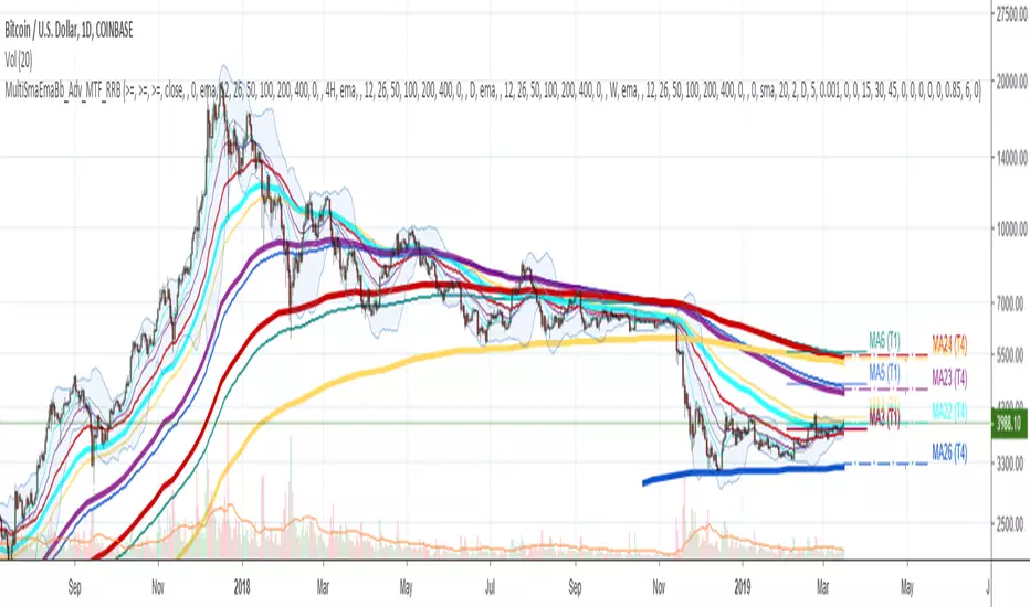
This indicator shows multiple MAs of any type SMA EMA WMA HMA etc with BB and MTF support, can show MAs as dynamically moving levels.
There are 4 MA groups + 1 BB group, a total of 4 TFs * 5 MAs = 20 MAs. You can assign any type/timeframe combo to a group, for example:
- EMAs 12,26,50,100,200 x H1, H4, D1, W1 (4 TFs x 5 MAs x 1 type)
- EMAs 8,10,13,21,30,50,55,100,200,400 x M15, H1 (2 TFs x 10 MAs x 1 type)
- D1 EMAs and SMAs 8,10,12,26,30,50,55,100,200,400 (1 TF x 10 MAs x 2 types)
- H1 WMAs 7,77,89,167,231; H4 HMAs 12,26,50,100,200; D1 EMAs 89,144,169,233,377; W1 SMAs 12,26,50,100,200 (4 TFs x 5 MAs x 4 types)
- +1 extra MA type/timeframe for BB
There are several versions: Simple, MTF, Pro MTF, Advanced MTF and Ultimate MTF. This is the Advanced MTF version. The Differences are listed below. All versions have BB
- Simple: you have 2 groups of MAs that can be assigned any type (5+5)
- MTF: +2 custom Timeframes for each group (2x5 MTF) +1 TF for BB, TF XY smoothing
- Pro MTF: 4 custom Timeframes for each group (4x3 MTF), 1 TF for BB, MA levels and show max bars back options
- Advanced MTF: +2 extra MAs/group (4x5 MTF), custom Ticker/Symbols, Timeframe <>= filter, Remove Duplicates Option
- Ultimate MTF: +individual settings for each MA, custom Ticker/Symbols
Features:
- 4x5 = 20 MAs of any type
- 4x MTF groups with XY step line smoothing
- +1 extra TF/type for BB MAs
- 4x5 = 20 MA levels with adjustable group offsets, indents and shift
- supports any existing type of MA: SMA, EMA, WMA, Hull Moving Average (HMA)
- custom tickers/symbols for each group - you can compare MAs of the same symbol across exchanges
- show max bars back option
- show/hide both groups of MAs/levels/BB and individual MAs
- timeframe filter: show only MAs/Levels with TFs <>= Current TF
- hide MAs/Levels with duplicate TFs
- support for custom TFs that are not available in free accounts: 2D, 3D etc
- support for timeframes in H: H, 2H, 4H etc
Notes:
- Uses timeframe textbox instead of input resolution dropdown to allow for 240 120 and other custom TFs
- Uses symbol textbox instead of input symbol to avoid establishing multiple dummy security connections to the current ticker - otherwise empty symbols will prevent script from running
- Possible reasons for missing MAs on a chart:
- there may not be enough bars in history to start plotting it. For example, W1 EMA200 needs at least 200 bars on a weekly chart.
- price << default Y smoothing step 5. For charts with low/fractional prices (i.e. 0.00002 << 5) adjust X Y smoothing as needed (set Y = 0.0000001) or disable it completely (set X,Y to 0,0)
- TradingView Replay Mode UI and Pinescript security calls are limited to TFs >= D (D,2D,W,MN...) for free accounts
- attempting to plot any TF < D1 in Replay Mode will only result in straight lines, but all TFs will work properly in history and real-time modes. This is not a bug.
- Max Bars Back (num_bars) is limited to 5000 for free accounts (10000 for paid), will show error when exceeded. To plot on all available history set to 0 (default)
- Slow load/redraw times. This indicator becomes slower, its UI less responsive when:
- Pinescript Node.js graphics library is too slow and inefficient at plotting bars/objects in a browser window. Code optimization doesn't help much - the graphics engine is the main reason for general slowness.
- the chart has a long history (10000+ bars) in a browser's cache (you have scrolled back a couple of screens in a max zoom mode).
- Reload the page/Load a fresh chart and then apply the indicator or
- Switch to another Timeframe (old TF history will still remain in cache and that TF will be slow)
- in max possible zoom mode around 4500 bars can fit on 1 screen - this also slows down responsiveness. Reset Zoom level
- initial load and redraw times after a param change in UI also depend on TF. For example:
D1/W1 - 2 sec, H1/H4 - 5-6 sec, M30 - 10 sec, M15/M5 - 4 sec, M1 - 5 sec.
M30 usually has the longest history (up to 16000 bars) and W1 - the shortest (1000 bars).
- when indicator uses more MAs (plots) and timeframes it will redraw slower. Seems that up to 5 Timeframes is acceptable, but 6+ Timeframes can become very slow.
- show_last=last_bars plot limit doesn't affect load/redraw times, so it was removed from MA plot
- Max Bars Back (num_bars) default/custom set UI value doesn't seem to affect load/redraw times
- In max zoom mode all dynamic levels disappear (they behave like text)
1. based on 3EmaBB, uses plot*, barssince and security functions
2. you can't set certain constants from input due to Pinescript limitations - change the code as needed, recompile and use as a private version
3. Levels = trackprice implementation
4. Show Max Bars Back = show_last implementation
5. swma has a fixed length = 4, alma and linreg have additional offset and smoothing params
6. Smoothing is applied by default for visual aesthetics on MTF. To use exact ma mtf values (lines with stair stepping) - disable it
Good Luck! You can explore, modify/reuse the code to build your own indicators.
Multifractal Forecast [ScorsoneEnterprises]Multifractal Forecast Indicator
The Multifractal Forecast is an indicator designed to model and forecast asset price movements using a multifractal framework. It uses concepts from fractal geometry and stochastic processes, specifically the Multifractal Model of Asset Returns (MMAR) and fractional Brownian motion (fBm), to generate price forecasts based on historical price data. The indicator visualizes potential future price paths as colored lines, providing traders with a probabilistic view of price trends over a specified trading time scale. Below is a detailed breakdown of the indicator’s functionality, inputs, calculations, and visualization.
Overview
Purpose: The indicator forecasts future price movements by simulating multiple price paths based on a multifractal model, which accounts for the complex, non-linear behavior of financial markets.
Key Concepts:
Multifractal Model of Asset Returns (MMAR): Models price movements as a multifractal process, capturing varying degrees of volatility and self-similarity across different time scales.
Fractional Brownian Motion (fBm): A generalization of Brownian motion that incorporates long-range dependence and self-similarity, controlled by the Hurst exponent.
Binomial Cascade: Used to model trading time, introducing heterogeneity in time scales to reflect market activity bursts.
Hurst Exponent: Measures the degree of long-term memory in the price series (persistence, randomness, or mean-reversion).
Rescaled Range (R/S) Analysis: Estimates the Hurst exponent to quantify the fractal nature of the price series.
Inputs
The indicator allows users to customize its behavior through several input parameters, each influencing the multifractal model and forecast generation:
Maximum Lag (max_lag):
Type: Integer
Default: 50
Minimum: 5
Purpose: Determines the maximum lag used in the rescaled range (R/S) analysis to calculate the Hurst exponent. A higher lag increases the sample size for Hurst estimation but may smooth out short-term dynamics.
2 to the n values in the Multifractal Model (n):
Type: Integer
Default: 4
Purpose: Defines the resolution of the multifractal model by setting the size of arrays used in calculations (N = 2^n). For example, n=4 results in N=16 data points. Larger n increases computational complexity and detail but may exceed Pine Script’s array size limits (capped at 100,000).
Multiplier for Binomial Cascade (m):
Type: Float
Default: 0.8
Purpose: Controls the asymmetry in the binomial cascade, which models trading time. The multiplier m (and its complement 2.0 - m) determines how mass is distributed across time scales. Values closer to 1 create more balanced cascades, while values further from 1 introduce more variability.
Length Scale for fBm (L):
Type: Float
Default: 100,000.0
Purpose: Scales the fractional Brownian motion output, affecting the amplitude of simulated price paths. Larger values increase the magnitude of forecasted price movements.
Cumulative Sum (cum):
Type: Integer (0 or 1)
Default: 1
Purpose: Toggles whether the fBm output is cumulatively summed (1=On, 0=Off). When enabled, the fBm series is accumulated to simulate a price path with memory, resembling a random walk with long-range dependence.
Trading Time Scale (T):
Type: Integer
Default: 5
Purpose: Defines the forecast horizon in bars (20 bars into the future). It also scales the binomial cascade’s output to align with the desired trading time frame.
Number of Simulations (num_simulations):
Type: Integer
Default: 5
Minimum: 1
Purpose: Specifies how many forecast paths are simulated and plotted. More simulations provide a broader range of possible price outcomes but increase computational load.
Core Calculations
The indicator combines several mathematical and statistical techniques to generate price forecasts. Below is a step-by-step explanation of its calculations:
Log Returns (lgr):
The indicator calculates log returns as math.log(close / close ) when both the current and previous close prices are positive. This measures the relative price change in a logarithmic scale, which is standard for financial time series analysis to stabilize variance.
Hurst Exponent Estimation (get_hurst_exponent):
Purpose: Estimates the Hurst exponent (H) to quantify the degree of long-term memory in the price series.
Method: Uses rescaled range (R/S) analysis:
For each lag from 2 to max_lag, the function calc_rescaled_range computes the rescaled range:
Calculate the mean of the log returns over the lag period.
Compute the cumulative deviation from the mean.
Find the range (max - min) of the cumulative deviation.
Divide the range by the standard deviation of the log returns to get the rescaled range.
The log of the rescaled range (log(R/S)) is regressed against the log of the lag (log(lag)) using the polyfit_slope function.
The slope of this regression is the Hurst exponent (H).
Interpretation:
H = 0.5: Random walk (no memory, like standard Brownian motion).
H > 0.5: Persistent behavior (trends tend to continue).
H < 0.5: Mean-reverting behavior (price tends to revert to the mean).
Fractional Brownian Motion (get_fbm):
Purpose: Generates a fractional Brownian motion series to model price movements with long-range dependence.
Inputs: n (array size 2^n), H (Hurst exponent), L (length scale), cum (cumulative sum toggle).
Method:
Computes covariance for fBm using the formula: 0.5 * (|i+1|^(2H) - 2 * |i|^(2H) + |i-1|^(2H)).
Uses Hosking’s method (referenced from Columbia University’s implementation) to generate fBm:
Initializes arrays for covariance (cov), intermediate calculations (phi, psi), and output.
Iteratively computes the fBm series by incorporating a random term scaled by the variance (v) and covariance structure.
Applies scaling based on L / N^H to adjust the amplitude.
Optionally applies cumulative summation if cum = 1 to produce a path with memory.
Output: An array of 2^n values representing the fBm series.
Binomial Cascade (get_binomial_cascade):
Purpose: Models trading time (theta) to account for non-uniform market activity (e.g., bursts of volatility).
Inputs: n (array size 2^n), m (multiplier), T (trading time scale).
Method:
Initializes an array of size 2^n with values of 1.0.
Iteratively applies a binomial cascade:
For each block (from 0 to n-1), splits the array into segments.
Randomly assigns a multiplier (m or 2.0 - m) to each segment, redistributing mass.
Normalizes the array by dividing by its sum and scales by T.
Checks for array size limits to prevent Pine Script errors.
Output: An array (theta) representing the trading time, which warps the fBm to reflect market activity.
Interpolation (interpolate_fbm):
Purpose: Maps the fBm series to the trading time scale to produce a forecast.
Method:
Computes the cumulative sum of theta and normalizes it to .
Interpolates the fBm series linearly based on the normalized trading time.
Ensures the output aligns with the trading time scale (T).
Output: An array of interpolated fBm values representing log returns over the forecast horizon.
Price Path Generation:
For each simulation (up to num_simulations):
Generates an fBm series using get_fbm.
Interpolates it with the trading time (theta) using interpolate_fbm.
Converts log returns to price levels:
Starts with the current close price.
For each step i in the forecast horizon (T), computes the price as prev_price * exp(log_return).
Output: An array of price levels for each simulation.
Visualization:
Trigger: Updates every T bars when the bar state is confirmed (barstate.isconfirmed).
Process:
Clears previous lines from line_array.
For each simulation, plots a line from the current bar’s close price to the forecasted price at bar_index + T.
Colors the line using a gradient (color.from_gradient) based on the final forecasted price relative to the minimum and maximum forecasted prices across all simulations (red for lower prices, teal for higher prices).
Output: Multiple colored lines on the chart, each representing a possible price path over the next T bars.
How It Works on the Chart
Initialization: On each bar, the indicator calculates the Hurst exponent (H) using historical log returns and prepares the trading time (theta) using the binomial cascade.
Forecast Generation: Every T bars, it generates num_simulations price paths:
Each path starts at the current close price.
Uses fBm to model log returns, warped by the trading time.
Converts log returns to price levels.
Plotting: Draws lines from the current bar to the forecasted price T bars ahead, with colors indicating relative price levels.
Dynamic Updates: The forecast updates every T bars, replacing old lines with new ones based on the latest price data and calculations.
Key Features
Multifractal Modeling: Captures complex market dynamics by combining fBm (long-range dependence) with a binomial cascade (non-uniform time).
Customizable Parameters: Allows users to adjust the forecast horizon, model resolution, scaling, and number of simulations.
Probabilistic Forecast: Multiple simulations provide a range of possible price outcomes, helping traders assess uncertainty.
Visual Clarity: Gradient-colored lines make it easy to distinguish bullish (teal) and bearish (red) forecasts.
Potential Use Cases
Trend Analysis: Identify potential price trends or reversals based on the direction and spread of forecast lines.
Risk Assessment: Evaluate the range of possible price outcomes to gauge market uncertainty.
Volatility Analysis: The Hurst exponent and binomial cascade provide insights into market persistence and volatility clustering.
Limitations
Computational Intensity: Large values of n or num_simulations may slow down execution or hit Pine Script’s array size limits.
Randomness: The binomial cascade and fBm rely on random terms (math.random), which may lead to variability between runs.
Assumptions: The model assumes log-normal price movements and fractal behavior, which may not always hold in extreme market conditions.
Adjusting Inputs:
Set max_lag based on the desired depth of historical analysis.
Adjust n for model resolution (start with 4–6 to avoid performance issues).
Tune m to control trading time variability (0.5–1.5 is typical).
Set L to scale the forecast amplitude (experiment with values like 10,000–1,000,000).
Choose T based on your trading horizon (20 for short-term, 50 for longer-term for example).
Select num_simulations for the number of forecast paths (5–10 is reasonable for visualization).
Interpret Output:
Teal lines suggest bullish scenarios, red lines suggest bearish scenarios.
A wide spread of lines indicates high uncertainty; convergence suggests a stronger trend.
Monitor Updates: Forecasts update every T bars, so check the chart periodically for new projections.
Chart Examples
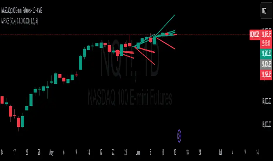
This is a daily AMEX:SPY chart with default settings. We see the simulations being done every T bars and they provide a range for us to analyze with a few simulations still in the range.
On this intraday PEPPERSTONE:COCOA chart I modified the Length Scale for fBm, L, parameter to be 1000 from 100000. Adjusting the parameter as you switch between timeframes can give you more contextual simulations.
On BITSTAMP:ETHUSD I modified the L to be 1000000 to have a more contextual set of simulations with crypto's volatile nature.
With L at 100000 we see the range for NASDAQ:TLT is correctly simulated. The recent pop stays within the bounds of the highest simulation. Note this is a cherry picked example to show the power and potential of these simulations.
Technical Notes
Error Handling: The script includes checks for array size limits and division by zero (math.abs(denominator) > 1e-10, v := math.max(v, 1e-10)).
External Reference: The fBm implementation is based on Hosking’s method (www.columbia.edu), ensuring a robust algorithm.
Conclusion
The Multifractal Forecast is a powerful tool for traders seeking to model complex market dynamics using a multifractal framework. By combining fBm, binomial cascades, and Hurst exponent analysis, it generates probabilistic price forecasts that account for long-range dependence and non-uniform market activity. Its customizable inputs and clear visualizations make it suitable for both technical analysis and strategy development, though users should be mindful of its computational demands and parameter sensitivity. For optimal use, experiment with input settings and validate forecasts against other technical indicators or market conditions.
Psych Level ScreenerThis Script is intended for Pine Screener and is not designed as a indicator!!!
Pine Screener is something TradingView has recently added and is still only a Beta version.
Pine Screener itself is currently only available to members that are Premium and above.
What it does:
This screener will actively look for tickers that are close to Pysch level in your watchlist.
Psych level here refers to price levels that are round numbers such as 50,100,1000.
Users can specify the offset from a psych level (in %) and scanner will scan for tickers that are within the offset. For example if offset is set at 5% then it will scan for tickers that are within +/-5% of a ticker. (for $100 psych level it will scan for ticker in $95-105 range)
Once scan is completed you will be able to see:
- Current price of ticker
- Closest psych level for that ticker
- % and $ move required for it to hit that psych level
- Ticker's day range and Average range (with % of average range completed for the day)
- Ticker volume and average volume
Setting up:
www.tradingview.com
Above link will help you guide how to setup Pine screener.
Use steps below to guide you the setup for this specific screener:
1. Open Pine Screener (open new tab, select screener the "Pine")
2. At the top, click on "Choose Indicator" and select "Psych Level Screener"
3. At the top again, click "Indicator Psych Level Screener" and select settings.
4. Change setting to your needs. Hit Apply when done.
a)"% offset from Psych Level" will scan for any stocks in your watchlist which are +/- from the offset you chose for any given psych level. Default is 5. (e.g. If offset is 5%, it will scan for stocks that are between $95-$105 vs $100 psych level, $190-$210 for $200 psych level and so on)
b) ATR length is number of previous trading days you want to include in your calculation. Moving Average Type is calculation method.
c) Rvol length is number of previous trading days you want to include in your calculation.
5. On top left, click "Price within specified offset of Psych. Level" and select true. Then select "Scan" which is located at the top next to "Indicator Psych Level Screener". This will filter out all the stock that meets the condition.
6. At the end of the column on the right there is a "+" symbol. From there you can add/remove columns. 30min/1hr/4hr/1D Trend are disabled by default so if this is needed please enable them.
7. You can change the order of ticker by ascending and descending order of each column label if needed. Just click on the arrow that comes up when you move the cursor to any of the column items.
8. You can specify advanced filter settings based on the variables in the column. (e.g., set price range of stock to filter out further) To do so, click on the column variable name in interest, located above the screener table (or right below "scan") and select "manual setup".
How to read the column:
Current Price: Shows current price of the ticker when scan was done. Currently Pine Screener does NOT support pre/post-hours data so no PM and AH price.
Psych Level: Psych level the current price is near to.
% to Psych Level: Price movement in % necessary to get to the Psych level.
$ to Psych Level: Price movement in $ necessary to get to the Psych level.
DTR: Daily True Range of the stock. i.e. High - Low of the ticker on the day.
ATR: Average True Range of stock in the last x days, where x is a value selected in the setting. (See step 3 in Previous section)
DTR vs ATR: Amount of DTR a ticker has done in % with respect to ATR. (e.g., 90% means DTR is 90% of ATR)
Vol.: Volume of a ticker for the day. Currently Pine Screener does NOT support pre/post-hours data so no PM and AH volume.
Avg. Vol: Average volume of a ticker in the last x days, where x is a value selected in the setting. (See step 3 in Previous section)
Rvol: Relative volume in percentage, measured by the ratio of day's volume and average volume.
30min/1hr/4hr/1D Trend: Trend status to see if the chart is Bullish or Bearish on each of the time frame. Bullishness or Bearishness is defined by the price being over or under the 34/50 cloud on each of the time frame. Output of 1 is Bullish, -1 is Bearish. 0 means price is sitting inside the 34/50 cloud. Currently Pine Screener does NOT support pre/post-hours data so 34/50 cloud is based on regular trading hours data ONLY.
Some things user should be aware of:
- Pine Screener itself is currently only available to TradingView members with Premium Subscription and above. (I can't to anything about this as this is NOT set by me, I have no control) For more info: www.tradingview.com
- The Pine Screener itself is a Beta version and this screener can stop working anytime depending on changes made by TradingView themselves. (Again I cannot control this)
- Pine Screener can only run on Watchlists for now. (as of 03/31/2025) You will have to prepare your own watchlists. In a Watchlist no more than 1000 tickers may be added. (This is TradingView rules)
- Psych level included are currently 50 to 1500 in steps of 50. If you need a specific number please let me know. Will add accordingly.
- Unfortunately this screener does not update automatically, so please hit "scan" to get latest screener result.
- I cannot add 10min trend to the column as Pine Screener does NOT support 10min timeframe as of now. (03/31/2025)
- This code is only meant for Pine Screener. I do NOT recommend using this as an indicator.
- Currently Pine Screener does NOT support pre/post-hours data. So data such as Price, Volume and EMA values are based on market hours data ONLY! (If I'm wrong about this please correct me / let me know and will make look into and make changes to the code)
Other useful links about Pine Screener:
Quick overview of the Screener’s functionality: www.tradingview.com
what do you need to know before you start working? : www.tradingview.com
These links will go over the setting up with GIFs so is easier to understand.
-----------------------------------------------------------------------------------------------------------------
If there are other column variables that you think is worth adding please let me know! Will try add it to the screener!
If you have any questions let me know as well, will reply soon as I can!
Have a good trading day and hope it helps!

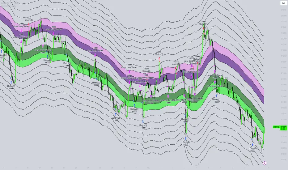
Honest Volatility Grid [Honestcowboy]The Honest Volatility Grid is an attempt at creating a robust grid trading strategy but without standard levels.
Normal grid systems use price levels like 1.01;1.02;1.03;1.04... and place an order at each of these levels. In this program instead we create a grid using keltner channels using a long term moving average.
🟦 IS THIS EVEN USEFUL?
The idea is to have a more fluid style of trading where levels expand and follow price and do not stick to precreated levels. This however also makes each closed trade different instead of using fixed take profit levels. In this strategy a take profit level can even be a loss. It is useful as a strategy because it works in a different way than most strategies, making it a good tool to diversify a portfolio of trading strategies.
🟦 STRATEGY
There are 10 levels below the moving average and 10 above the moving average. For each side of the moving average the strategy uses 1 to 3 orders maximum (3 shorts at top, 3 longs at bottom). For instance you buy at level 2 below moving average and you increase position size when level 6 is reached (a cheaper price) in order to spread risks.
By default the strategy exits all trades when the moving average is reached, this makes it a mean reversion strategy. It is specifically designed for the forex market as these in my experience exhibit a lot of ranging behaviour on all the timeframes below daily.
There is also a stop loss at the outer band by default, in case price moves too far from the mean.
What are the risks?
In case price decides to stay below the moving average and never reaches the outer band one trade can create a very substantial loss, as the bands will keep following price and are not at a fixed level.
Explanation of default parameters
By default the strategy uses a starting capital of 25000$, this is realistic for retail traders.
Lot sizes at each level are set to minimum lot size 0.01, there is no reason for the default to be risky, if you want to risk more or increase equity curve increase the number at your own risk.
Slippage set to 20 points: that's a normal 2 pip slippage you will find on brokers.
Fill limit assumtion 20 points: so it takes 2 pips to confirm a fill, normal forex spread.
Commission is set to 0.00005 per contract: this means that for each contract traded there is a 5$ or whatever base currency pair has as commission. The number is set to 0.00005 because pinescript does not know that 1 contract is 100000 units. So we divide the number by 100000 to get a realistic commission.
The script will also multiply lot size by 100000 because pinescript does not know that lots are 100000 units in forex.
Extra safety limit
Normally the script uses strategy.exit() to exit trades at TP or SL. But because these are created 1 bar after a limit or stop order is filled in pinescript. There are strategy.orders set at the outer boundaries of the script to hedge against that risk. These get deleted bar after the first order is filled. Purely to counteract news bars or huge spikes in price messing up backtest.
🟦 VISUAL GOODIES
I've added a market profile feature to the edge of the grid. This so you can see in which grid zone market has been the most over X bars in the past. Some traders may wish to only turn on the strategy whenever the market profile displays specific characteristics (ranging market for instance).
These simply count how many times a high, low, or close price has been in each zone for X bars in the past. it's these purple boxes at the right side of the chart.
🟦 Script can be fully automated to MT5
There are risk settings in lot sizes or % for alerts and symbol settings provided at the bottom of the indicator. The script will send alert to MT5 broker trying to mimic the execution that happens on tradingview. There are always delays when using a bridge to MT5 broker and there could be errors so be mindful of that. This script sends alerts in format so they can be read by tradingview.to which is a bridge between the platforms.
Use the all alert function calls feature when setting up alerts and make sure you provide the right webhook if you want to use this approach.
Almost every setting in this indicator has a tooltip added to it. So if any setting is not clear hover over the (?) icon on the right of the setting.
Chande Kroll Trend Strategy (SPX, 1H) | PINEINDICATORSThe "Chande Kroll Stop Strategy" is designed to optimize trading on the SPX using a 1-hour timeframe. This strategy effectively combines the Chande Kroll Stop indicator with a Simple Moving Average (SMA) to create a robust method for identifying long entry and exit points. This detailed description will explain the components, rationale, and usage to ensure compliance with TradingView's guidelines and help traders understand the strategy's utility and application.
Objective
The primary goal of this strategy is to identify potential long trading opportunities in the SPX by leveraging volatility-adjusted stop levels and trend-following principles. It aims to capture upward price movements while managing risk through dynamically calculated stops.
Chande Kroll Stop Parameters:
Calculation Mode: Offers "Linear" and "Exponential" options for position size calculation. The default mode is "Exponential."
Risk Multiplier: An adjustable multiplier for risk management and position sizing, defaulting to 5.
ATR Period: Defines the period for calculating the Average True Range (ATR), with a default of 10.
ATR Multiplier: A multiplier applied to the ATR to set stop levels, defaulting to 3.
Stop Length: Period used to determine the highest high and lowest low for stop calculation, defaulting to 21.
SMA Length: Period for the Simple Moving Average, defaulting to 21.
Calculation Details:
ATR Calculation: ATR is calculated over the specified period to measure market volatility.
Chande Kroll Stop Calculation:
High Stop: The highest high over the stop length minus the ATR multiplied by the ATR multiplier.
Low Stop: The lowest low over the stop length plus the ATR multiplied by the ATR multiplier.
SMA Calculation: The 21-period SMA of the closing price is used as a trend filter.
Entry and Exit Conditions:
Long Entry: A long position is initiated when the closing price crosses over the low stop and is above the 21-period SMA. This condition ensures that the market is trending upward and that the entry is made in the direction of the prevailing trend.
Exit Long: The long position is exited when the closing price falls below the high stop, indicating potential downward movement and protecting against significant drawdowns.
Position Sizing:
The quantity of shares to trade is calculated based on the selected calculation mode (linear or exponential) and the risk multiplier. This ensures position size is adjusted dynamically based on current market conditions and user-defined risk tolerance.
Exponential Mode: Quantity is calculated using the formula: riskMultiplier / lowestClose * 1000 * strategy.equity / strategy.initial_capital.
Linear Mode: Quantity is calculated using the formula: riskMultiplier / lowestClose * 1000.
Execution:
When the long entry condition is met, the strategy triggers a buy signal, and a long position is entered with the calculated quantity. An alert is generated to notify the trader.
When the exit condition is met, the strategy closes the position and triggers a sell signal, accompanied by an alert.
Plotting:
Buy Signals: Indicated with an upward triangle below the bar.
Sell Signals: Indicated with a downward triangle above the bar.
Application
This strategy is particularly effective for trading the SPX on a 1-hour timeframe, capitalizing on price movements by adjusting stop levels dynamically based on market volatility and trend direction.
Default Setup
Initial Capital: $1,000
Risk Multiplier: 5
ATR Period: 10
ATR Multiplier: 3
Stop Length: 21
SMA Length: 21
Commission: 0.01
Slippage: 3 Ticks
Backtesting Results
Backtesting indicates that the "Chande Kroll Stop Strategy" performs optimally on the SPX when applied to the 1-hour timeframe. The strategy's dynamic adjustment of stop levels helps manage risk effectively while capturing significant upward price movements. Backtesting was conducted with a realistic initial capital of $1,000, and commissions and slippage were included to ensure the results are not misleading.
Risk Management
The strategy incorporates risk management through dynamically calculated stop levels based on the ATR and a user-defined risk multiplier. This approach ensures that position sizes are adjusted according to market volatility, helping to mitigate potential losses. Trades are sized to risk a sustainable amount of equity, adhering to the guideline of risking no more than 5-10% per trade.
Usage Notes
Customization: Users can adjust the ATR period, ATR multiplier, stop length, and SMA length to better suit their trading style and risk tolerance.
Alerts: The strategy includes alerts for buy and sell signals to keep traders informed of potential entry and exit points.
Pyramiding: Although possible, the strategy yields the best results without pyramiding.
Justification of Components
The Chande Kroll Stop indicator and the 21-period SMA are combined to provide a robust framework for identifying long trading opportunities in trending markets. Here is why they work well together:
Chande Kroll Stop Indicator: This indicator provides dynamic stop levels that adapt to market volatility, allowing traders to set logical stop-loss levels that account for current price movements. It is particularly useful in volatile markets where fixed stops can be easily hit by random price fluctuations. By using the ATR, the stop levels adjust based on recent market activity, ensuring they remain relevant in varying market conditions.
21-Period SMA: The 21-period SMA acts as a trend filter to ensure trades are taken in the direction of the prevailing market trend. By requiring the closing price to be above the SMA for long entries, the strategy aligns itself with the broader market trend, reducing the risk of entering trades against the overall market direction. This helps to avoid false signals and ensures that the trades are in line with the dominant market movement.
Combining these two components creates a balanced approach that captures trending price movements while protecting against significant drawdowns through adaptive stop levels. The Chande Kroll Stop ensures that the stops are placed at levels that reflect current volatility, while the SMA filter ensures that trades are only taken when the market is trending in the desired direction.
Concepts Underlying Calculations
ATR (Average True Range): Used to measure market volatility, which informs the stop levels.
SMA (Simple Moving Average): Used to filter trades, ensuring positions are taken in the direction of the trend.
Chande Kroll Stop: Combines high and low price levels with ATR to create dynamic stop levels that adapt to market conditions.
Risk Disclaimer
Trading involves substantial risk, and most day traders incur losses. The "Chande Kroll Stop Strategy" is provided for informational and educational purposes only. Past performance is not indicative of future results. Users are advised to adjust and personalize this trading strategy to better match their individual trading preferences and risk tolerance.

WEEKLY BTC TRADING SCRYPTWeekly BTC Trading Scrypt(WBTS)
This script is only suggested for cryptocurrencies and weekly buying strategy which is long term.Using it in another markets(e.g forex,stock,e.t.c) is not suggested. The thing makes it different than other strategies we try to understand bull and bear seasons and buying selected crypto currency as using formula if weekly closing value crossover eight weeks simple moving avarage buy,else if selected crypto currency's weekly closing value crossunder eight weeks simple avarage sell. Eight week moving avarage is also uses weekly closing prices but for being able to use this strategy ,trading pair must have more than eight candles in weekly chart otherwise the 8 weeks simple moving avarage value cannot be calculated and script does not work.
This script has a chart called WBTS and it has following features:
Strategy group consist of 3 inputs:
1)Source: Close by default. Our whole strategy uses close values. You can change it but not suggested.
2)Loss Ratio: Because of the cases like the circumstances that manipulates market or high volatility , sometimes graphic show wrong buying signals and this ratio saves user from big money looses(Note : This ratio will always work when selling condition occurs to make user take his profit or prevent him to loss more money because of a wrong positive comes from the indicator.)
3)Reward Ratio : When selling condition happens it will exit user with more profit(if price is already higher than buying point) otherwise it will dimunish loss a bit(if user is below of buying point) or prevents looses(if user is in buying point when selling condition happened.
MA group consist of 2 inputs:
COLOR:Specifies color of the moving avarage.It is equal to #FF3232by hex color code by default.
LINE WIDTH: Specifies linewidth of the moving avarage. It is 2 by default.
GRAPHIC group consist of 2 inputs:
COLOR: It specifies the color of the line which consist of weekly closing prices. It is equal to #6666FF hex color code by default.
LINE WIDTH: Specifies linewidth of the line which consist of weekly closing prices. It is 2 by default.
STRATEGY EXECUTION YEAR: It will show the orders,profits and looses done by script after the input year giving in it.It is 2020 by default.
The last feature is strategy equity,it is not in one of these groups. User should click on settings button on the WBTS indicator than chose Style section and there is a deactivated check box near in the plot section if user activate it, the equity line will show in indicator's graph.
Logic of This Strategy:The story of this strategy began when I studied BTC's price movement from 2020 to today with 8 weeks simple moving avarage (it takes weekly closes as source) and weekly clossing values. I understood that there was a perfect interest between bull and bear market and following conditions:
buy_condition=crossover(weekly_closing_values,8_week_simple_moving_avarage)
sell_condition=crossover(weekly_closing_values,8_week_simple_moving_avarage)
and I tried same thing on the same and bigger time frames("for example i studied how the strategy works from the beginning to today with bitcoin and what is our final equity") with bitcoin and other cryptocurrencies and this made me saw better the relation between giving conditions and general market psychology, however I also witnessed some wrong positives coming by script and used a risk reward ratio to save user and set risk reward ratio 1/3 after a research.
For both conditions(buy_condition and sell_condition),when they are realised,script will alert users and an order will be triggered.
Before finishing the description,from settings/properties/ user can set initial capital,base currency,order size and type,but it is 100000 for initial_amount and 1 contract for order size by default.
In backtesting I used the options like the following example :
Initial capital=1000
Base_curreny=USD
Order size=40 USD
Properties place must set different by every single user according to his or her capital and order size must not be higher than his total money because this script is not the best or a good script for derivatives. It is only written for long term-crypto spot trading and I strongly recommend to users that margin may cause bad results and please do not use it with any margin or any market different than crypto market.
Thank you very much for reading)

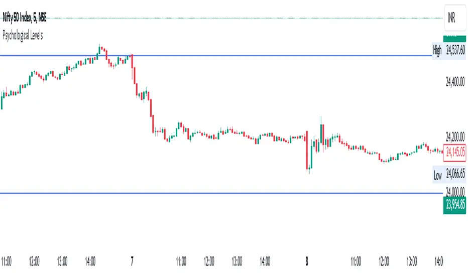
Psychological Levels- Rounding Numbers Psychological Levels Indicator
Overview:
The Psychological Levels Indicator automatically identifies and plots significant price levels based on psychological thresholds, which are key areas where market participants often focus their attention. These levels act as potential support or resistance zones due to human behavioral tendencies to round off numbers. This indicator dynamically adjusts the levels based on the stock's price range and ensures seamless visibility across the chart.
Key Features:
Dynamic Step Sizes:
The indicator adjusts the levels dynamically based on the stock price:
For prices below 500: Levels are spaced at 10.
For prices between 500 and 3000: Levels are spaced at 50, 100, and 1000.
For prices between 3000 and 10,000: Levels are spaced at 100 and 1000.
For prices above 10,000: Levels are spaced at 500 and 1000.
Extended Visibility:
The plotted levels are extended across the entire chart for improved visualization, ensuring traders can easily monitor these critical zones over time.
Customization Options:
Line Color: Choose the color for the levels to suit your charting style.
Line Style: Select from solid, dashed, or dotted lines.
Line Width: Adjust the thickness of the lines for better clarity.
Clean and Efficient Design:
The indicator only plots levels relevant to the visible chart range, avoiding unnecessary clutter and ensuring a clean workspace.
How It Works:
It calculates the relevant step sizes based on the price:
Smaller step sizes for lower-priced stocks.
Larger step sizes for higher-priced stocks.
Primary, secondary, and (if applicable) tertiary levels are plotted dynamically:
Primary Levels: The most granular levels based on the stock price.
Secondary Levels: Higher-order levels for broader significance.
Tertiary Levels: Additional levels for lower-priced stocks to enhance detail.
These levels are plotted across the chart, allowing traders to visualize key psychological areas effortlessly.
Use Cases:
Day Trading: Identify potential intraday support and resistance levels.
Swing Trading: Recognize key price zones where trends may pause or reverse.
Long-Term Investing: Gain insights into significant price zones for entry or exit strategies.
ROI Levels IndicatorROI Levels Indicator 📈💰
Description: The "ROI Levels Indicator" helps you visualize key Return on Investment (ROI) levels directly on your chart, making it easier to track your profit milestones! 🚀 This tool allows you to enter your entry price, and it calculates levels from 100% up to 1000% ROI, each with a spread to represent potential support and resistance zones. The levels are visually represented by red rectangles to help identify zones where the market might react. This is a great way for traders to easily understand profit-taking points and psychological price levels!
Features:
🛠️ Custom Entry Price: Set your own entry price to start calculating ROI levels.
📊 Multiple ROI Levels: Levels from 100% to 1000%, with a customizable spread for visual clarity.
🔴 Visual Representation: Each level is marked with a full-screen-width rectangle and label, making it easy to track.
🚨 Entry Price Plot: A red dashed line marks your entry price for easy reference.
How to Use:
Enter Your Price: Use the "Entry Price" input field to specify the entry price of your trade.
Spread Adjustment: Adjust the spread percentage if you want more or less tolerance around each ROI level.
View the Levels: The script automatically plots 100% to 1000% ROI levels. Each level is represented by a red rectangle and labeled on the right side for quick identification.
Track Profit Zones: Use the plotted ROI levels to identify key profit-taking areas or potential zones of support and resistance.
Pro Tip: Use these levels as reference points to decide when to scale out of positions or manage risk effectively! 🎯
Happy trading, and may your ROI always be on the rise! 📈🔥

Statistics • Chi Square • P-value • SignificanceThe Statistics • Chi Square • P-value • Significance publication aims to provide a tool for combining different conditions and checking whether the outcome is significant using the Chi-Square Test and P-value.
🔶 USAGE
The basic principle is to compare two or more groups and check the results of a query test, such as asking men and women whether they want to see a romantic or non-romantic movie.
–––––––––––––––––––––––––––––––––––––––––––––
| | ROMANTIC | NON-ROMANTIC | ⬅︎ MOVIE |
–––––––––––––––––––––––––––––––––––––––––––––
| MEN | 2 | 8 | 10 |
–––––––––––––––––––––––––––––––––––––––––––––
| WOMEN | 7 | 3 | 10 |
–––––––––––––––––––––––––––––––––––––––––––––
|⬆︎ SEX | 10 | 10 | 20 |
–––––––––––––––––––––––––––––––––––––––––––––
We calculate the Chi-Square Formula, which is:
Χ² = Σ ( (Observed Value − Expected Value)² / Expected Value )
In this publication, this is:
chiSquare = 0.
for i = 0 to rows -1
for j = 0 to colums -1
observedValue = aBin.get(i).aFloat.get(j)
expectedValue = math.max(1e-12, aBin.get(i).aFloat.get(colums) * aBin.get(rows).aFloat.get(j) / sumT) //Division by 0 protection
chiSquare += math.pow(observedValue - expectedValue, 2) / expectedValue
Together with the 'Degree of Freedom', which is (rows − 1) × (columns − 1) , the P-value can be calculated.
In this case it is P-value: 0.02462
A P-value lower than 0.05 is considered to be significant. Statistically, women tend to choose a romantic movie more, while men prefer a non-romantic one.
Users have the option to choose a P-value, calculated from a standard table or through a math.ucla.edu - Javascript-based function (see references below).
Note that the population (10 men + 10 women = 20) is small, something to consider.
Either way, this principle is applied in the script, where conditions can be chosen like rsi, close, high, ...
🔹 CONDITION
Conditions are added to the left column ('CONDITION')
For example, previous rsi values (rsi ) between 0-100, divided in separate groups
🔹 CLOSE
Then, the movement of the last close is evaluated
UP when close is higher then previous close (close )
DOWN when close is lower then previous close
EQUAL when close is equal then previous close
It is also possible to use only 2 columns by adding EQUAL to UP or DOWN
UP
DOWN/EQUAL
or
UP/EQUAL
DOWN
In other words, when previous rsi value was between 80 and 90, this resulted in:
19 times a current close higher than previous close
14 times a current close lower than previous close
0 times a current close equal than previous close
However, the P-value tells us it is not statistical significant.
NOTE: Always keep in mind that past behaviour gives no certainty about future behaviour.
A vertical line is drawn at the beginning of the chosen population (max 4990)
Here, the results seem significant.
🔹 GROUPS
It is important to ensure that the groups are formed correctly. All possibilities should be present, and conditions should only be part of 1 group.
In the example above, the two top situations are acceptable; close against close can only be higher, lower or equal.
The two examples at the bottom, however, are very poorly constructed.
Several conditions can be placed in more than 1 group, and some conditions are not integrated into a group. Even if the results are significant, they are useless because of the group formation.
A population count is added as an aid to spot errors in group formation.
In this example, there is a discrepancy between the population and total count due to the absence of a condition.
The results when rsi was between 5-25 are not included, resulting in unreliable results.
🔹 PRACTICAL EXAMPLES
In this example, we have specific groups where the condition only applies to that group.
For example, the condition rsi > 55 and rsi <= 65 isn't true in another group.
Also, every possible rsi value (0 - 100) is present in 1 of the groups.
rsi > 15 and rsi <= 25 28 times UP, 19 times DOWN and 2 times EQUAL. P-value: 0.01171
When looking in detail and examining the area 15-25 RSI, we see this:
The population is now not representative (only checking for RSI between 15-25; all other RSI values are not included), so we can ignore the P-value in this case. It is merely to check in detail. In this case, the RSI values 23 and 24 seem promising.
NOTE: We should check what the close price did without any condition.
If, for example, the close price had risen 100 times out of 100, this would make things very relative.
In this case (at least two conditions need to be present), we set 1 condition at 'always true' and another at 'always false' so we'll get only the close values without any condition:
Changing the population or the conditions will change the P-value.
In the following example, the outcome is evaluated when:
close value from 1 bar back is higher than the close value from 2 bars back
close value from 1 bar back is lower/equal than the close value from 2 bars back
Or:
close value from 1 bar back is higher than the close value from 2 bars back
close value from 1 bar back is equal than the close value from 2 bars back
close value from 1 bar back is lower than the close value from 2 bars back
In both examples, all possibilities of close against close are included in the calculations. close can only by higher, equal or lower than close
Both examples have the results without a condition included (5 = 5 and 5 < 5) so one can compare the direction of current close.
🔶 NOTES
• Always keep in mind that:
Past behaviour gives no certainty about future behaviour.
Everything depends on time, cycles, events, fundamentals, technicals, ...
• This test only works for categorical data (data in categories), such as Gender {Men, Women} or color {Red, Yellow, Green, Blue} etc., but not numerical data such as height or weight. One might argue that such tests shouldn't use rsi, close, ... values.
• Consider what you're measuring
For example rsi of the current bar will always lead to a close higher than the previous close, since this is inherent to the rsi calculations.
• Be careful; often, there are na -values at the beginning of the series, which are not included in the calculations!
• Always keep in mind considering what the close price did without any condition
• The numbers must be large enough. Each entry must be five or more. In other words, it is vital to make the 'population' large enough.
• The code can be developed further, for example, by splitting UP, DOWN in close UP 1-2%, close UP 2-3%, close UP 3-4%, ...
• rsi can be supplemented with stochRSI, MFI, sma, ema, ...
🔶 SETTINGS
🔹 Population
• Choose the population size; in other words, how many bars you want to go back to. If fewer bars are available than set, this will be automatically adjusted.
🔹 Inputs
At least two conditions need to be chosen.
• Users can add up to 11 conditions, where each condition can contain two different conditions.
🔹 RSI
• Length
🔹 Levels
• Set the used levels as desired.
🔹 Levels
• P-value: P-value retrieved using a standard table method or a function.
• Used function, derived from Chi-Square Distribution Function; JavaScript
LogGamma(Z) =>
S = 1
+ 76.18009173 / Z
- 86.50532033 / (Z+1)
+ 24.01409822 / (Z+2)
- 1.231739516 / (Z+3)
+ 0.00120858003 / (Z+4)
- 0.00000536382 / (Z+5)
(Z-.5) * math.log(Z+4.5) - (Z+4.5) + math.log(S * 2.50662827465)
Gcf(float X, A) => // Good for X > A +1
A0=0., B0=1., A1=1., B1=X, AOLD=0., N=0
while (math.abs((A1-AOLD)/A1) > .00001)
AOLD := A1
N += 1
A0 := A1+(N-A)*A0
B0 := B1+(N-A)*B0
A1 := X*A0+N*A1
B1 := X*B0+N*B1
A0 := A0/B1
B0 := B0/B1
A1 := A1/B1
B1 := 1
Prob = math.exp(A * math.log(X) - X - LogGamma(A)) * A1
1 - Prob
Gser(X, A) => // Good for X < A +1
T9 = 1. / A
G = T9
I = 1
while (T9 > G* 0.00001)
T9 := T9 * X / (A + I)
G := G + T9
I += 1
G *= math.exp(A * math.log(X) - X - LogGamma(A))
Gammacdf(x, a) =>
GI = 0.
if (x<=0)
GI := 0
else if (x
Chisqcdf = Gammacdf(Z/2, DF/2)
Chisqcdf := math.round(Chisqcdf * 100000) / 100000
pValue = 1 - Chisqcdf
🔶 REFERENCES
mathsisfun.com, Chi-Square Test
Chi-Square Distribution Function

Volume Profile with a few polylinesThe base of "Volume Profile with a few polylines" is another script of mine, Volume Profile (Maps) .
The structure of maps is used to gather the data. However, the drawings is done with polylines.
This enables coders to draw an entire volume profile with just a few polylines, while the range is broader.
This results in the benefit to draw more "lines" than with line.new() / box.new() alone.
🔶 CONCEPTS
🔹 Polylines
polyline.new creates a new polyline instance and displays it on the chart, sequentially connecting all of the points in the `points` array with line segments.
The segments in the drawing can be straight or curved depending on the `curved` parameter.
In this script, points are connected, starting from the bottom. The created line moves up until there is a price level where a volume value needs to be displayed,
at which the line goes to the left to the concerning volume value, coming back at the same price level until the line returns to its initial x-axis,
after which the line will continue to rise until all values are displayed.
A polyline can contain maximum 10000 points (10K).
Since the line has to go back and forth, each price/volume line takes 3 points.
In the case that 20K bars all have a different price, we would need 60K points, or just 6 polylines. A maximum of 100 polylines can be displayed.
The 3 highest volume values are displayed with line.new(), each with their own colour.
🔹 Maps
A map object is a collection that consists of key - value pairs
Each key is unique and can only appear once. When adding a new value with a key that the map already contains, that value replaces the old value associated with the key .
You can change the value of a particular key though, for example adding volume (value) at the same price (key), the latter technique is used in this script.
Volume is added to the map, associated with a particular price (default close, can be set at high, low, open,...)
When the map already contains the same price (key), the value (volume) is added to the existing volume at the associated price.
A map can contain maximum 50K values, which is more than enough to hold 20K bars (Basic 5K - Premium plan 20K), so the whole history can be put into a map.
🔹 Rounding function
This publication contains 2 round functions, which can be used to widen the Volume Profile
Round
• "Round" set at zero -> nothing changes to the source number
• "Round" set below zero -> x digit(s) after the decimal point, starting from the right side, and rounded.
• "Round" set above zero -> x digit(s) before the decimal point, starting from the right side, and rounded.
Example: 123456.789
0->123456.789
1->123456.79
2->123456.8
3->123457
-1->123460
-2->123500
Step
Another option is custom steps.
After setting "Round" to "Step", choose the desired steps in price,
Examples
• 2 -> 1234.00, 1236.00, 1238.00, 1240.00
• 5 -> 1230.00, 1235.00, 1240.00, 1245.00
• 100 -> 1200.00, 1300.00, 1400.00, 1500.00
• 0.05 -> 1234.00, 1234.05, 1234.10, 1234.15
•••
🔶 FEATURES
🔹 Volume * currency
Let's take as example BTCUSD, relative to USD, 10 volume at a price of 100 BTCUSD will be very different than 10 volume at a price of 30000 (1K vs. 300K)
If you want volume to be associated with USD, enable Volume * currency . Volume will then be multiplied by the price:
• 10 volume, 1 BTC = 100 -> 1000
• 10 volume, 1 BTC = 30K -> 300K
Polylines has the attributes curved & closed.
When "curved" is enabled the drawing will connect all points from the `points` array using curved line segments.
When "closed" is enabled the drawing will also connect the first point to the last point from the `points` array, resulting in a closed polyline.
They are default disabled, but can be enabled:
🔶 DETAILS
🔹 Put
When the map doesn't contain a price, it will be added, using map.put(id, key, value)
In our code:
map.put(originalMap, price, volume)
or
originalMap.put(price, volume)
A key (price) is now associated with a value (volume) -> key : value
Since all keys are unique, we don't have to know its position to extract the value, we just need to know the key -> map.get(id, key)
We use map.get() when a certain key already exists in the map, and we want to add volume with that value.
if originalMap.contains(price)
originalMap.put(price, originalMap.get(price) + volume)
-> At the last bar, all prices (source) are now associated with volume.
🔶 SETTINGS
Source : Set source of choice; default close , can be set as high , low , open , ...
Volume & currency : Enable to multiply volume with price (see Features )
Amount of bars : Set amount of bars which you want to include in the Volume Profile
🔹 Round -> ' Round/Step '
Round -> see Concepts
Step -> see Concepts
🔹 Display Volume Profile
Offset: shifts the Volume Profile (max. 500 bars to the right of last bar, see Features )
Max width Volume Profile: largest volume will be x bars wide, the rest is displayed as a ratio against largest volume (see Features )
Colours
Curved: make lines curved
Closed: connect last with first point
🔶 LIMITATIONS
• Lines won't go further than first bar (coded).
• The Volume Profile can be placed maximum 500 bar to the right of last price.

EMA RSI Strategy
Simple strategy
=============
If the last two closes are in ascending order, the rsi is below 50 and ascending, and the current candle is above 200 ema, then LONG. If the last two closes are in descending order, the rsi is above 50 and descending, and the current candle is below 200 ema, then SHORT.
LONG Exit strategy:
ATR: Last 14 day
Lowest: The lowest value of the last 14 candles
Limit points = (Trade Price - Lowest + ATR) * 100000
trail_points : Limit/2
trail_offset = Limit/2
SHORT Exit strategy:
ATR: Last 14 day
Highest: The higher value of the last 14 candles
Limit points = (Trade Price - Highest + ATR) * 100000
trail_points : Limit/2
trail_offset = Limit/2
Backtest results for the AUDUSD pair gave positive results over the last three months.
I am testing this strategy using a python bot in a real environment this week and will update the results at the end of the week.
Disclaimer
This is not financial advice. You should seek independent advice to check how the strategy information relates to your unique circumstances.
We are not liable for any loss caused, whether due to negligence or otherwise arising from the use of, or reliance on, the information provided directly or indirectly by this strategy.

inwCoin Average Position Price Calculator - For CryptocurrencyEver wonder what is my average entry ?
No need to use excel.
Just use this simple indicator to calculate average entry of your multiple positions.
How to use
--------------
1) Just input your entries into each box. ( Buy price + buy amount )
2) If you don't want to use any input, just uncheck the checkbox.
How to read value
----------------------
- This indicator will calculate the asset amount you got when you purchase it, by asset amount = entry amount / entry price ( Eg. buy BTC at 10,000$ per BTC with 1,000 USD = 1000/10000 = 0.1 BTC )
- It will calculate your current value of the asset you holding and compare it with all of the money you already invested. Also the profit/loss.
- It will show the average entry price with the green line on the chart and in the textbox.

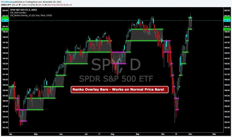
CM Renko Overlay BarsCM_Renko Overlay Bars V1
Overlays Renko Bars on Regular Price Bars.
Default Renko plot is based on Average True Range. Look Back period adjustable in Inputs Tab.
If you Choose to use "Traditional" Renko bars and pick the Size of the Renko Bars the please read below.
Value in Input Tab is multiplied by .001 (To work on Forex)
1 = 10 pips on EURUSD - 1 X .001 = .001 or 10 Pips
10 = .01 or 100 Pips
1000 = 1 point to the left of decimal. 1 Point in Stocks etc.
10000 = 10 Points on Stocks etc.
***V2 will fix this issue.
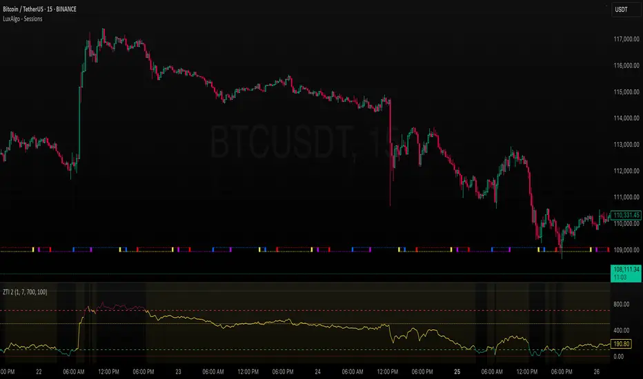
ZLEMA Trend Index 2.0ZTI — ZLEMA Trend Index 2.0 (0–1000)
Overview
Price Mapped ZTI v2.0 - Enhanced Zero-Lag Trend Index.
This indicator is a significant upgrade to the original ZTI v1.0, featuring enhanced resolution from 0-100 to 0-1000 levels for dramatically improved price action accuracy. The Price Mapped ZTI uses direct price-to-level mapping to eliminate statistical noise and provide true proportional representation of market movements.
Key Innovation: Instead of statistical normalization, this version maps current price position within a user-defined lookback period directly to the ZTI scale, ensuring perfect correlation with actual price movements. I believe this is the best way to capture trends instead of directly on the charts using a plethora of indicators which introduces bad signals resulting in drawdowns. The RSI-like ZTI overbought and oversold lines filter valid trends by slicing through the current trading zone. Unlike RSI that can introduce false signals, the ZTI levels 1 to 1000 is faithfully mapped to the lowest to highest price in the current trading zone (lookback period in days) which can be changed in the settings. The ZTI line will never go off the beyond the ZTI levels in case of extreme trend continuation as the trading zone is constantly updated to reflect only the most recent bars based on lookback days.
Core Features
✅ 10x Higher Resolution - 0-1000 scale provides granular movement detection
✅ Adjustable Trading Zone - Customizable lookback period from 1-50 days
✅ Price-Proportional Mapping - Direct correlation between price position and ZTI level
✅ Zero Statistical Lag - No rolling averages or standard deviation calculations
✅ Multi-Strategy Adaptability - Single parameter adjustment for different trading styles
Trading Zone Optimization
📊 Lookback Period Strategies
Short-term (1-3 days):
Ultra-responsive to recent price action
Perfect for scalping and day trading
Tight range produces more sensitive signals
Medium-term (7-14 days):
Balanced view of recent trading range
Ideal for swing trading
Captures meaningful support/resistance levels
Long-term (21-30 days):
Broader market context
Excellent for position trading
Smooths out short-term market noise
⚡ Market Condition Adaptation
Volatile Markets: Use shorter lookback (3-5 days) for tighter ranges
Trending Markets: Use longer lookback (14-21 days) for broader context
Ranging Markets: Use medium lookback (7-10 days) for clear boundaries
🎯 Timeframe Optimization
1-minute charts: 1-2 day lookback
5-minute charts: 2-5 day lookback
Hourly charts: 7-14 day lookback
Daily charts: 21-50 day lookback
Trading Applications
Scalping Setup (2-day lookback):
Super tight range for quick reversals
ZTI 800+ = immediate short opportunity
ZTI 200- = immediate long opportunity
Swing Trading Setup (10-day lookback):
Meaningful swing levels captured
ZTI extremes = high-probability reversal zones
More stable signals, reduced whipsaws
Advanced Usage
🔧 Real-Time Adaptability
Trending days: Increase to 14+ days for broader perspective
Range-bound days: Decrease to 3 days for tighter signals
High volatility: Shorter lookback for responsiveness
Low volatility: Longer lookback to avoid false signals
💡 Multi-Timeframe Approach
Entry signals: Use 7-day ZTI on main timeframe
Trend confirmation: Use 21-day ZTI on higher timeframe
Exit timing: Use 3-day ZTI for precise exits
🌐 Session Optimization
Asian session: Shorter lookback (3-5 days) for range-bound conditions
London/NY session: Longer lookback (7-14 days) for trending conditions
How It Works
The indicator maps the current price position within the specified lookback period directly to a 0-1000 scale and plots it using ZLEMA (Zero Lag Exponential Moving Average) which has the least lag of the available popular moving averages:
Price at recent high = ZTI at 1000
Price at recent low = ZTI at 1
Price at mid-range = ZTI at 500
This creates perfect proportional representation where every price movement translates directly to corresponding ZTI movement, eliminating the false signals common in traditional oscillators.
This single, versatile indicator adapts to any market condition, timeframe, or trading style through one simple parameter adjustment, making it an essential tool for traders at every level.
Credits
ZLEMA techniques widely attributed to John Ehlers.
Disclaimer
This tool is for educational purposes only and is not financial advice. Backtest and forward‑test before live use, and always manage risk.
Please note that I set this as closed source to prevent source code cloning by others, repackaging and republishing which results in multiple confusing choices of the same indicator.
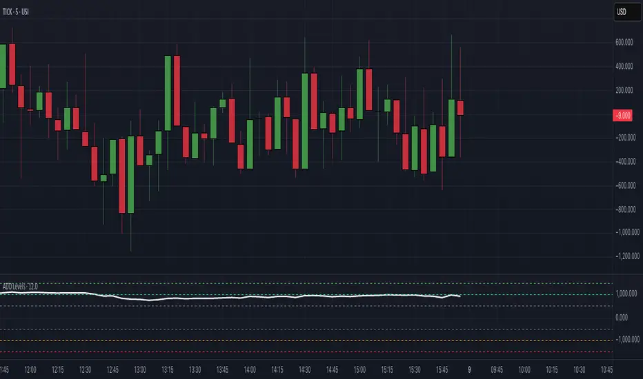
$ADD LevelsThis Pine Script is designed to track and visualize the NYSE Advance-Decline Line (ADD). The Advance-Decline Line is a popular market breadth indicator, showing the difference between advancing and declining stocks on the NYSE. It’s often used to gauge overall market sentiment and strength.
1. //@version=5
This line tells TradingView to use Pine Script v5, the latest and most powerful version of Pine.
2. indicator(" USI:ADD Levels", overlay=false)
• This creates a new indicator called ” USI:ADD Levels”.
• overlay=false means it will appear in a separate pane, not on the main price chart.
3. add = request.security(...)
This fetches real-time data from the symbol USI:ADD (Advance-Decline Line) using a 1-minute timeframe. You can change the timeframe if needed.
add_symbol = input.symbol(" USI:ADD ", "Market Breadth Symbol")
add = request.security(add_symbol, "1", close)
4. Key Thresholds
These define the market sentiment zones:
Zone. Value. Meaning
Overbought +1500 Extremely bullish
Bullish +1000 Generally bullish trend
Neutral ±500 Choppy, unclear market
Bearish -1000 Generally bearish trend
Oversold -1500 Extremely bearish
5. Plot the ADD Line hline(...)
Draws static lines at +1500, +1000, +500, -500, -1000, -1500 for reference so you can visually assess where ADD stands.
6. Horizontal Threshold Lines bgcolor(...)
• Green background if ADD > +1500 → extremely bullish.
• Red background if ADD < -1500 → extremely bearish.
7. Background Highlights alertcondition(...)
• Green background if ADD > +1500 → extremely bullish.
• Red background if ADD < -1500 → extremely bearish.
8. Alert Conditions. alertcondition(...)
Lets you create automatic alerts for:
• USI:ADD being very high or low.
• Crosses above +1000 (bullish trigger).
• Crosses below -1000 (bearish trigger).
You can use these to trigger trades or monitor sentiment shifts.
Summary: When to Use It
• Use this script in a market breadth dashboard.
• Combine it with price action and volume analysis.
• Monitor for ADD crosses to signal potential market reversals or momentum.
Stx Monthly Trades ProfitMonthly profit displays profits in a grid and allows you to know the gain related to the investment during each month.
The profit could be computed in terms of gain/trade_cost or as percentage of equity update.
Settings:
- Profit: Monthly profit percentage or percentage of equity
- Table position
This strategy is intended only as a container for the code and for testing the script of the profit table.
Setting of strategy allows to select the test case for this snippet (percentage grid).
Money management: not relevant as strategy is a test case.
This script stand out as take in account the gain of each trade in relation to the capital invested in each trade. For example consider the following scenario:
Capital of 1000$ and we invest a fixed amount of 1000$ (I know is too risky but is a good example), we gain 10% every month.
After 10 months our capital is of 2000$ and our strategy is perfect as we have the same performance every month.
Instead, evaluating the percentage of equity we have 10% the first month, 9.9% the second (1200$/1100$ - 1) and 5.26% the tenth month. So seems that strategy degrade with times but this is not true.
For this reason, to evaluate my strategy I prefer to see the montly return of investment.
WARNING: The strategy provided with this script is only a test case and allows to see the behavior with different "trades" management, for these reason commision are set to zero.
At the moment only the provided test cases are handled:
test 1 - single entry and single exit;
test 2 - single entry and multiple exits;
test 3 - single entry and switch position;
Ruckard TradingLatinoThis strategy tries to mimic TradingLatino strategy.
The current implementation is beta.
Si hablas castellano o espanyol por favor consulta MENSAJE EN CASTELLANO más abajo.
It's aimed at BTCUSDT pair and 4h timeframe.
STRATEGY DEFAULT SETTINGS EXPLANATION
max_bars_back=5000 : This is a random number of bars so that the strategy test lasts for one or two years
calc_on_order_fills=false : To wait for the 4h closing is too much. Try to check if it's worth entering a position after closing one. I finally decided not to recheck if it's worth entering after an order is closed. So it is false.
calc_on_every_tick=false
pyramiding=0 : We only want one entry allowed in the same direction. And we don't want the order to scale by error.
initial_capital=1000 : These are 1000 USDT. By using 1% maximum loss per trade and 7% as a default stop loss by using 1000 USDT at 12000 USDT per BTC price you would entry with around 142 USDT which are converted into: 0.010 BTC . The maximum number of decimal for contracts on this BTCUSDT market is 3 decimals. E.g. the minimum might be: 0.001 BTC . So, this minimal 1000 amount ensures us not to entry with less than 0.001 entries which might have happened when using 100 USDT as an initial capital.
slippage=1 : Binance BTCUSDT mintick is: 0.01. Binance slippage: 0.1 % (Let's assume). TV has an integer slippage. It does not have a percentage based slippage. If we assume a 1000 initial capital, the recommended equity is 142 which at 11996 USDT per BTC price means: 0.011 BTC. The 0.1% slippage of: 0.011 BTC would be: 0.000011 . This is way smaller than the mintick. So our slippage is going to be 1. E.g. 1 (slippage) * 0.01 (mintick)
commission_type=strategy.commission.percent and commission_value=0.1 : According to: binance . com / en / fee / schedule in VIP 0 level both maker and taker fees are: 0.1 %.
BACKGROUND
Jaime Merino is a well known Youtuber focused on crypto trading
His channel TradingLatino
features monday to friday videos where he explains his strategy.
JAIME MERINO STANCE ON BOTS
Jaime Merino stance on bots (taken from memory out of a 2020 June video from him):
'~
You know. They can program you a bot and it might work.
But, there are some special situations that the bot would not be able to handle.
And, I, as a human, I would handle it. And the bot wouldn't do it.
~'
My long term target with this strategy script is add as many
special situations as I can to the script
so that it can match Jaime Merino behaviour even in non normal circumstances.
My alternate target is learn Pine script
and enjoy programming with it.
WARNING
This script might be bigger than other TradingView scripts.
However, please, do not be confused because the current status is beta.
This script has not been tested with real money.
This is NOT an official strategy from Jaime Merino.
This is NOT an official strategy from TradingLatino . net .
HOW IT WORKS
It basically uses ADX slope and LazyBear's Squeeze Momentum Indicator
to make its buy and sell decisions.
Fast paced EMA being bigger than slow paced EMA
(on higher timeframe) advices going long.
Fast paced EMA being smaller than slow paced EMA
(on higher timeframe) advices going short.
It finally add many substrats that TradingLatino uses.
SETTINGS
__ SETTINGS - Basics
____ SETTINGS - Basics - ADX
(ADX) Smoothing {14}
(ADX) DI Length {14}
(ADX) key level {23}
____ SETTINGS - Basics - LazyBear Squeeze Momentum
(SQZMOM) BB Length {20}
(SQZMOM) BB MultFactor {2.0}
(SQZMOM) KC Length {20}
(SQZMOM) KC MultFactor {1.5}
(SQZMOM) Use TrueRange (KC) {True}
____ SETTINGS - Basics - EMAs
(EMAS) EMA10 - Length {10}
(EMAS) EMA10 - Source {close}
(EMAS) EMA55 - Length {55}
(EMAS) EMA55 - Source {close}
____ SETTINGS - Volume Profile
Lowest and highest VPoC from last three days
is used to know if an entry has a support
VPVR of last 100 4h bars
is also taken into account
(VP) Use number of bars (not VP timeframe): Uses 'Number of bars {100}' setting instead of 'Volume Profile timeframe' setting for calculating session VPoC
(VP) Show tick difference from current price {False}: BETA . Might be useful for actions some day.
(VP) Number of bars {100}: If 'Use number of bars (not VP timeframe)' is turned on this setting is used to calculate session VPoC.
(VP) Volume Profile timeframe {1 day}: If 'Use number of bars (not VP timeframe)' is turned off this setting is used to calculate session VPoC.
(VP) Row width multiplier {0.6}: Adjust how the extra Volume Profile bars are shown in the chart.
(VP) Resistances prices number of decimal digits : Round Volume Profile bars label numbers so that they don't have so many decimals.
(VP) Number of bars for bottom VPOC {18}: 18 bars equals 3 days in suggested timeframe of 4 hours. It's used to calculate lowest session VPoC from previous three days. It's also used as a top VPOC for sells.
(VP) Ignore VPOC bottom advice on long {False}: If turned on it ignores bottom VPOC (or top VPOC on sells) when evaluating if a buy entry is worth it.
(VP) Number of bars for VPVR VPOC {100}: Number of bars to calculate the VPVR VPoC. We use 100 as Jaime once used. When the price bounces back to the EMA55 it might just bounce to this VPVR VPoC if its price it's lower than the EMA55 (Sells have inverse algorithm).
____ SETTINGS - ADX Slope
ADX Slope
help us to understand if ADX
has a positive slope, negative slope
or it is rather still.
(ADXSLOPE) ADX cut {23}: If ADX value is greater than this cut (23) then ADX has strength
(ADXSLOPE) ADX minimum steepness entry {45}: ADX slope needs to be 45 degrees to be considered as a positive one.
(ADXSLOPE) ADX minimum steepness exit {45}: ADX slope needs to be -45 degrees to be considered as a negative one.
(ADXSLOPE) ADX steepness periods {3}: In order to avoid false detection the slope is calculated along 3 periods.
____ SETTINGS - Next to EMA55
(NEXTEMA55) EMA10 to EMA55 bounce back percentage {80}: EMA10 might bounce back to EMA55 or maybe to 80% of its complete way to EMA55
(NEXTEMA55) Next to EMA55 percentage {15}: How much next to the EMA55 you need to be to consider it's going to bounce back upwards again.
____ SETTINGS - Stop Loss and Take Profit
You can set a default stop loss or a default take profit.
(STOPTAKE) Stop Loss % {7.0}
(STOPTAKE) Take Profit % {2.0}
____ SETTINGS - Trailing Take Profit
You can customize the default trailing take profit values
(TRAILING) Trailing Take Profit (%) {1.0}: Trailing take profit offset in percentage
(TRAILING) Trailing Take Profit Trigger (%) {2.0}: When 2.0% of benefit is reached then activate the trailing take profit.
____ SETTINGS - MAIN TURN ON/OFF OPTIONS
(EMAS) Ignore advice based on emas {false}.
(EMAS) Ignore advice based on emas (On closing long signal) {False}: Ignore advice based on emas but only when deciding to close a buy entry.
(SQZMOM) Ignore advice based on SQZMOM {false}: Ignores advice based on SQZMOM indicator.
(ADXSLOPE) Ignore advice based on ADX positive slope {false}
(ADXSLOPE) Ignore advice based on ADX cut (23) {true}
(STOPTAKE) Take Profit? {false}: Enables simple Take Profit.
(STOPTAKE) Stop Loss? {True}: Enables simple Stop Loss.
(TRAILING) Enable Trailing Take Profit (%) {True}: Enables Trailing Take Profit.
____ SETTINGS - Strategy mode
(STRAT) Type Strategy: 'Long and Short', 'Long Only' or 'Short Only'. Default: 'Long and Short'.
____ SETTINGS - Risk Management
(RISKM) Risk Management Type: 'Safe', 'Somewhat safe compound' or 'Unsafe compound'. ' Safe ': Calculations are always done with the initial capital (1000) in mind. The maximum losses per trade/day/week/month are taken into account. ' Somewhat safe compound ': Calculations are done with initial capital (1000) or a higher capital if it increases. The maximum losses per trade/day/week/month are taken into account. ' Unsafe compound ': In each order all the current capital is gambled and only the default stop loss per order is taken into account. That means that the maximum losses per trade/day/week/month are not taken into account. Default : 'Somewhat safe compound'.
(RISKM) Maximum loss per trade % {1.0}.
(RISKM) Maximum loss per day % {6.0}.
(RISKM) Maximum loss per week % {8.0}.
(RISKM) Maximum loss per month % {10.0}.
____ SETTINGS - Decimals
(DECIMAL) Maximum number of decimal for contracts {3}: How small (3 decimals means 0.001) an entry position might be in your exchange.
EXTRA 1 - PRICE IS IN RANGE indicator
(PRANGE) Print price is in range {False}: Enable a bottom label that indicates if the price is in range or not.
(PRANGE) Price range periods {5}: How many previous periods are used to calculate the medians
(PRANGE) Price range maximum desviation (%) {0.6} ( > 0 ): Maximum positive desviation for range detection
(PRANGE) Price range minimum desviation (%) {0.6} ( > 0 ): Mininum negative desviation for range detection
EXTRA 2 - SQUEEZE MOMENTUM Desviation indicator
(SQZDIVER) Show degrees {False}: Show degrees of each Squeeze Momentum Divergence lines to the x-axis.
(SQZDIVER) Show desviation labels {False}: Whether to show or not desviation labels for the Squeeze Momentum Divergences.
(SQZDIVER) Show desviation lines {False}: Whether to show or not desviation lines for the Squeeze Momentum Divergences.
EXTRA 3 - VOLUME PROFILE indicator
WARNING: This indicator works not on current bar but on previous bar. So in the worst case it might be VP from 4 hours ago. Don't worry, inside the strategy calculus the correct values are used. It's just that I cannot show the most recent one in the chart.
(VP) Print recent profile {False}: Show Volume Profile indicator
(VP) Avoid label price overlaps {False}: Avoid label prices to overlap on the chart.
EXTRA 4 - ZIGNALY SUPPORT
(ZIG) Zignaly Alert Type {Email}: 'Email', 'Webhook'. ' Email ': Prepare alert_message variable content to be compatible with zignaly expected email content format. ' Webhook ': Prepare alert_message variable content to be compatible with zignaly expected json content format.
EXTRA 5 - DEBUG
(DEBUG) Enable debug on order comments {False}: If set to true it prepares the order message to match the alert_message variable. It makes easier to debug what would have been sent by email or webhook on each of the times an order is triggered.
HOW TO USE THIS STRATEGY
BOT MODE: This is the default setting.
PROPER VOLUME PROFILE VIEWING: Click on this strategy settings. Properties tab. Make sure Recalculate 'each time the order was run' is turned off.
NEWBIE USER: (Check PROPER VOLUME PROFILE VIEWING above!) You might want to turn on the 'Print recent profile {False}' setting. Alternatively you can use my alternate realtime study: 'Resistances and supports based on simplified Volume Profile' but, be aware, it might consume one indicator.
ADVANCED USER 1: Turn on the 'Print price is in range {False}' setting and help us to debug this subindicator. Also help us to figure out how to include this value in the strategy.
ADVANCED USER 2: Turn on the all the (SQZDIVER) settings and help us to figure out how to include this value in the strategy.
ADVANCED USER 3: (Check PROPER VOLUME PROFILE VIEWING above!) Turn on the 'Print recent profile {False}' setting and report any problem with it.
JAIME MERINO: Just use the indicator as it comes by default. It should only show BUY signals, SELL signals and their associated closing signals. From time to time you might want to check 'ADVANCED USER 2' instructions to check that there's actually a divergence. Check also 'ADVANCED USER 1' instructions for your amusement.
EXTRA ADVICE
It's advised that you use this strategy in addition to these two other indicators:
* Squeeze Momentum Indicator
* ADX
so that your chart matches as close as possible to TradingLatino chart.
ZIGNALY INTEGRATION
This strategy supports Zignaly email integration by default. It also supports Zignaly Webhook integration.
ZIGNALY INTEGRATION - Email integration example
What you would write in your alert message:
||{{strategy.order.alert_message}}||key=MYSECRETKEY||
ZIGNALY INTEGRATION - Webhook integration example
What you would write in your alert message:
{ {{strategy.order.alert_message}} , "key" : "MYSECRETKEY" }
CREDITS
I have reused and adapted some code from
'Directional Movement Index + ADX & Keylevel Support' study
which it's from TradingView console user.
I have reused and adapted some code from
'3ema' study
which it's from TradingView hunganhnguyen1193 user.
I have reused and adapted some code from
'Squeeze Momentum Indicator ' study
which it's from TradingView LazyBear user.
I have reused and adapted some code from
'Strategy Tester EMA-SMA-RSI-MACD' study
which it's from TradingView fikira user.
I have reused and adapted some code from
'Support Resistance MTF' study
which it's from TradingView LonesomeTheBlue user.
I have reused and adapted some code from
'TF Segmented Linear Regression' study
which it's from TradingView alexgrover user.
I have reused and adapted some code from
"Poor man's volume profile" study
which it's from TradingView IldarAkhmetgaleev user.
FEEDBACK
Please check the strategy source code for more detailed information
where, among others, I explain all of the substrats
and if they are implemented or not.
Q1. Did I understand wrong any of the Jaime substrats (which I have implemented)?
Q2. The strategy yields quite profit when we should long (EMA10 from 1d timeframe is higher than EMA55 from 1d timeframe.
Why the strategy yields much less profit when we should short (EMA10 from 1d timeframe is lower than EMA55 from 1d timeframe)?
Any idea if you need to do something else rather than just reverse what Jaime does when longing?
FREQUENTLY ASKED QUESTIONS
FAQ1. Why are you giving this strategy for free?
TradingLatino and his fellow enthusiasts taught me this strategy. Now I'm giving back to them.
FAQ2. Seriously! Why are you giving this strategy for free?
I'm confident his strategy might be improved a lot. By keeping it to myself I would avoid other people contributions to improve it.
Now that everyone can contribute this is a win-win.
FAQ3. How can I connect this strategy to my Exchange account?
It seems that you can attach alerts to strategies.
You might want to combine it with a paying account which enable Webhook URLs to work.
I don't know how all of this works right now so I cannot give you advice on it.
You will have to do your own research on this subject. But, be careful. Automating trades, if not done properly,
might end on you automating losses.
FAQ4. I have just found that this strategy by default gives more than 3.97% of 'maximum series of losses'. That's unacceptable according to my risk management policy.
You might want to reduce default stop loss setting from 7% to something like 5% till you are ok with the 'maximum series of losses'.
FAQ5. Where can I learn more about your work on this strategy?
Check the source code. You might find unused strategies. Either because there's not a substantial increases on earnings. Or maybe because they have not been implemented yet.
FAQ6. How much leverage is applied in this strategy?
No leverage.
FAQ7. Any difference with original Jaime Merino strategy?
Most of the times Jaime defines an stop loss at the price entry. That's not the case here. The default stop loss is 7% (but, don't be confused it only means losing 1% of your investment thanks to risk management). There's also a trailing take profit that triggers at 2% profit with a 1% trailing.
FAQ8. Why this strategy return is so small?
The strategy should be improved a lot. And, well, backtesting in this platform is not guaranteed to return theoric results comparable to real-life returns. That's why I'm personally forward testing this strategy to verify it.
MENSAJE EN CASTELLANO
En primer lugar se agradece feedback para mejorar la estrategia.
Si eres un usuario avanzado y quieres colaborar en mejorar el script no dudes en comentar abajo.
Ten en cuenta que aunque toda esta descripción tenga que estar en inglés no es obligatorio que el comentario esté en inglés.
CHISTE - CASTELLANO
¡Pero Jaime!
¡400.000!
¡Tu da mun!
MACD StrategyOverview
The "MACD Strategy" is a straightforward trading strategy tested for BTCUSDT Futures on the 1-minute timeframe, leveraging the Moving Average Convergence Divergence (MACD) indicator to identify momentum-based buy and sell opportunities. Developed with input from expert trading analyst insights, this strategy combines technical precision with risk management, making it suitable for traders of all levels on platforms like TradingView. It focuses on capturing trend reversals and momentum shifts, with clear visual cues and automated alerts for seamless integration with trading bots (e.g., Bitget webhooks).
#### How It Works
This strategy uses the MACD indicator to generate trading signals based on momentum and trend direction:
- **Buy Signal**: Triggered when the MACD line crosses above the signal line, and the MACD histogram turns positive (above zero). This suggests increasing bullish momentum.
- **Sell Signal**: Triggered when the MACD line crosses below the signal line, and the MACD histogram turns negative (below zero), indicating growing bearish momentum.
Once a signal is detected, the strategy opens a position (long for buy, short for sell) with a position size calculated based on your risk tolerance. It includes a stop-loss to limit losses and a take-profit to lock in gains, both dynamically adjusted using the Average True Range (ATR) for adaptability to market volatility.
#### Key Features
- **MACD-Based Signals**: Relies solely on MACD for entry points, plotted in a separate pane for clear momentum analysis.
- **Risk Management**: Automatically calculates position size based on a percentage of your account balance and sets stop-loss and take-profit levels using ATR multipliers and a risk:reward ratio.
- **Visual Feedback**: Plots entry, stop-loss, and take-profit lines on the chart with labeled markers for easy tracking.
- **Alerts**: Includes Bitget webhook-compatible alerts for automated trading, notifying you of buy and sell signals in real-time.
#### Input Parameters
- **Account Balance**: Default 10000 – Set your initial trading capital to determine position sizing.
- **MACD Fast Length**: Default 12 – The short-term EMA period for MACD sensitivity.
- **MACD Slow Length**: Default 26 – The long-term EMA period for MACD calculation.
- **MACD Signal Length**: Default 9 – The smoothing period for the signal line.
- **Risk Per Trade (%)**: Default 3.0 – The percentage of your account balance risked per trade (e.g., 3% of 10000 = 300).
- **Risk:Reward Ratio**: Default 3.0 – The ratio of potential profit to risk (e.g., 3:1 means risking 1 to gain 3).
- **SL Multiplier**: Default 1.0 – Multiplies ATR to set the stop-loss distance (e.g., 1.0 x ATR).
- **TP Multiplier**: Default 3.0 – Multiplies ATR to set the take-profit distance, adjusted by the risk:reward ratio.
- **Line Length (bars)**: Default 25 – Duration in bars for displaying trade lines on the chart.
- **Label Position**: Default 'left' – Position of text labels (left or right) relative to trade lines.
- **ATR Period**: Default 14 – The number of periods for calculating ATR to measure volatility.
#### How to Use
1. **Add to Chart**: Load the "MACD Strategy" as a strategy and the "MACD Indicator" as a separate indicator on your TradingView chart (recommended for BTCUSDT Futures on the 1-minute timeframe).
2. **Customize Settings**: Adjust the input parameters based on your risk tolerance and market conditions. For BTCUSDT Futures, consider reducing `Risk Per Trade (%)` during high volatility (e.g., 1%) or increasing `SL Multiplier` for wider stops.
3. **Visual Analysis**: Watch the main chart for trade entry lines (green for buy, red for sell), stop-loss (red), and take-profit (green) lines with labels. Use the MACD pane below to confirm momentum shifts.
4. **Set Alerts**: Create alerts in TradingView for "Buy Signal" and "Sell Signal" to automate trades via Bitget webhooks.
5. **Backtest and Optimize**: Test the strategy on historical BTCUSDT Futures 1-minute data to fine-tune parameters. The short timeframe requires quick execution, so monitor closely for slippage or latency.
#### Tips for Success
- **Market Conditions**: This strategy performs best in trending markets on the 1-minute timeframe. Avoid choppy conditions where MACD crossovers may produce false signals.
- **Risk Management**: Start with the default 3% risk per trade and adjust downward (e.g., 1%) during volatile periods like BTCUSDT news events. The 3:1 risk:reward ratio targets consistent profitability.
- **Timeframe**: Optimized for 1-minute charts; switch to 5-minute or 15-minute for less noise if needed.
- **Confirmation**: Cross-check MACD signals with price action or support/resistance levels for higher accuracy on BTCUSDT Futures.
#### Limitations
- This strategy relies solely on MACD, so it may lag in fast-moving or sideways markets. Consider adding a secondary filter (e.g., RSI) if needed.
- Stop-loss and take-profit are ATR-based and may need adjustment for BTCUSDT Futures’ high volatility, especially during leverage trading.
#### Conclusion
The "MACD Strategy" offers a simple yet effective way to trade momentum shifts using the MACD indicator, tested for BTCUSDT Futures on the 1-minute timeframe, with robust risk management and visual tools. Whether you’re scalping crypto futures or exploring short-term trends, this strategy provides a solid foundation for automated or manual trading. Share your feedback or customizations in the comments, and happy trading!

Kelly Position Size CalculatorThis position sizing calculator implements the Kelly Criterion, developed by John L. Kelly Jr. at Bell Laboratories in 1956, to determine mathematically optimal position sizes for maximizing long-term wealth growth. Unlike arbitrary position sizing methods, this tool provides a scientifically solution based on your strategy's actual performance statistics and incorporates modern refinements from over six decades of academic research.
The Kelly Criterion addresses a fundamental question in capital allocation: "What fraction of capital should be allocated to each opportunity to maximize growth while avoiding ruin?" This question has profound implications for financial markets, where traders and investors constantly face decisions about optimal capital allocation (Van Tharp, 2007).
Theoretical Foundation
The Kelly Criterion for binary outcomes is expressed as f* = (bp - q) / b, where f* represents the optimal fraction of capital to allocate, b denotes the risk-reward ratio, p indicates the probability of success, and q represents the probability of loss (Kelly, 1956). This formula maximizes the expected logarithm of wealth, ensuring maximum long-term growth rate while avoiding the risk of ruin.
The mathematical elegance of Kelly's approach lies in its derivation from information theory. Kelly's original work was motivated by Claude Shannon's information theory (Shannon, 1948), recognizing that maximizing the logarithm of wealth is equivalent to maximizing the rate of information transmission. This connection between information theory and wealth accumulation provides a deep theoretical foundation for optimal position sizing.
The logarithmic utility function underlying the Kelly Criterion naturally embodies several desirable properties for capital management. It exhibits decreasing marginal utility, penalizes large losses more severely than it rewards equivalent gains, and focuses on geometric rather than arithmetic mean returns, which is appropriate for compounding scenarios (Thorp, 2006).
Scientific Implementation
This calculator extends beyond basic Kelly implementation by incorporating state of the art refinements from academic research:
Parameter Uncertainty Adjustment: Following Michaud (1989), the implementation applies Bayesian shrinkage to account for parameter estimation error inherent in small sample sizes. The adjustment formula f_adjusted = f_kelly × confidence_factor + f_conservative × (1 - confidence_factor) addresses the overconfidence bias documented by Baker and McHale (2012), where the confidence factor increases with sample size and the conservative estimate equals 0.25 (quarter Kelly).
Sample Size Confidence: The reliability of Kelly calculations depends critically on sample size. Research by Browne and Whitt (1996) provides theoretical guidance on minimum sample requirements, suggesting that at least 30 independent observations are necessary for meaningful parameter estimates, with 100 or more trades providing reliable estimates for most trading strategies.
Universal Asset Compatibility: The calculator employs intelligent asset detection using TradingView's built-in symbol information, automatically adapting calculations for different asset classes without manual configuration.
ASSET SPECIFIC IMPLEMENTATION
Equity Markets: For stocks and ETFs, position sizing follows the calculation Shares = floor(Kelly Fraction × Account Size / Share Price). This straightforward approach reflects whole share constraints while accommodating fractional share trading capabilities.
Foreign Exchange Markets: Forex markets require lot-based calculations following Lot Size = Kelly Fraction × Account Size / (100,000 × Base Currency Value). The calculator automatically handles major currency pairs with appropriate pip value calculations, following industry standards described by Archer (2010).
Futures Markets: Futures position sizing accounts for leverage and margin requirements through Contracts = floor(Kelly Fraction × Account Size / Margin Requirement). The calculator estimates margin requirements as a percentage of contract notional value, with specific adjustments for micro-futures contracts that have smaller sizes and reduced margin requirements (Kaufman, 2013).
Index and Commodity Markets: These markets combine characteristics of both equity and futures markets. The calculator automatically detects whether instruments are cash-settled or futures-based, applying appropriate sizing methodologies with correct point value calculations.
Risk Management Integration
The calculator integrates sophisticated risk assessment through two primary modes:
Stop Loss Integration: When fixed stop-loss levels are defined, risk calculation follows Risk per Trade = Position Size × Stop Loss Distance. This ensures that the Kelly fraction accounts for actual risk exposure rather than theoretical maximum loss, with stop-loss distance measured in appropriate units for each asset class.
Strategy Drawdown Assessment: For discretionary exit strategies, risk estimation uses maximum historical drawdown through Risk per Trade = Position Value × (Maximum Drawdown / 100). This approach assumes that individual trade losses will not exceed the strategy's historical maximum drawdown, providing a reasonable estimate for strategies with well-defined risk characteristics.
Fractional Kelly Approaches
Pure Kelly sizing can produce substantial volatility, leading many practitioners to adopt fractional Kelly approaches. MacLean, Sanegre, Zhao, and Ziemba (2004) analyze the trade-offs between growth rate and volatility, demonstrating that half-Kelly typically reduces volatility by approximately 75% while sacrificing only 25% of the growth rate.
The calculator provides three primary Kelly modes to accommodate different risk preferences and experience levels. Full Kelly maximizes growth rate while accepting higher volatility, making it suitable for experienced practitioners with strong risk tolerance and robust capital bases. Half Kelly offers a balanced approach popular among professional traders, providing optimal risk-return balance by reducing volatility significantly while maintaining substantial growth potential. Quarter Kelly implements a conservative approach with low volatility, recommended for risk-averse traders or those new to Kelly methodology who prefer gradual introduction to optimal position sizing principles.
Empirical Validation and Performance
Extensive academic research supports the theoretical advantages of Kelly sizing. Hakansson and Ziemba (1995) provide a comprehensive review of Kelly applications in finance, documenting superior long-term performance across various market conditions and asset classes. Estrada (2008) analyzes Kelly performance in international equity markets, finding that Kelly-based strategies consistently outperform fixed position sizing approaches over extended periods across 19 developed markets over a 30-year period.
Several prominent investment firms have successfully implemented Kelly-based position sizing. Pabrai (2007) documents the application of Kelly principles at Berkshire Hathaway, noting Warren Buffett's concentrated portfolio approach aligns closely with Kelly optimal sizing for high-conviction investments. Quantitative hedge funds, including Renaissance Technologies and AQR, have incorporated Kelly-based risk management into their systematic trading strategies.
Practical Implementation Guidelines
Successful Kelly implementation requires systematic application with attention to several critical factors:
Parameter Estimation: Accurate parameter estimation represents the greatest challenge in practical Kelly implementation. Brown (1976) notes that small errors in probability estimates can lead to significant deviations from optimal performance. The calculator addresses this through Bayesian adjustments and confidence measures.
Sample Size Requirements: Users should begin with conservative fractional Kelly approaches until achieving sufficient historical data. Strategies with fewer than 30 trades may produce unreliable Kelly estimates, regardless of adjustments. Full confidence typically requires 100 or more independent trade observations.
Market Regime Considerations: Parameters that accurately describe historical performance may not reflect future market conditions. Ziemba (2003) recommends regular parameter updates and conservative adjustments when market conditions change significantly.
Professional Features and Customization
The calculator provides comprehensive customization options for professional applications:
Multiple Color Schemes: Eight professional color themes (Gold, EdgeTools, Behavioral, Quant, Ocean, Fire, Matrix, Arctic) with dark and light theme compatibility ensure optimal visibility across different trading environments.
Flexible Display Options: Adjustable table size and position accommodate various chart layouts and user preferences, while maintaining analytical depth and clarity.
Comprehensive Results: The results table presents essential information including asset specifications, strategy statistics, Kelly calculations, sample confidence measures, position values, risk assessments, and final position sizes in appropriate units for each asset class.
Limitations and Considerations
Like any analytical tool, the Kelly Criterion has important limitations that users must understand:
Stationarity Assumption: The Kelly Criterion assumes that historical strategy statistics represent future performance characteristics. Non-stationary market conditions may invalidate this assumption, as noted by Lo and MacKinlay (1999).
Independence Requirement: Each trade should be independent to avoid correlation effects. Many trading strategies exhibit serial correlation in returns, which can affect optimal position sizing and may require adjustments for portfolio applications.
Parameter Sensitivity: Kelly calculations are sensitive to parameter accuracy. Regular calibration and conservative approaches are essential when parameter uncertainty is high.
Transaction Costs: The implementation incorporates user-defined transaction costs but assumes these remain constant across different position sizes and market conditions, following Ziemba (2003).
Advanced Applications and Extensions
Multi-Asset Portfolio Considerations: While this calculator optimizes individual position sizes, portfolio-level applications require additional considerations for correlation effects and aggregate risk management. Simplified portfolio approaches include treating positions independently with correlation adjustments.
Behavioral Factors: Behavioral finance research reveals systematic biases that can interfere with Kelly implementation. Kahneman and Tversky (1979) document loss aversion, overconfidence, and other cognitive biases that lead traders to deviate from optimal strategies. Successful implementation requires disciplined adherence to calculated recommendations.
Time-Varying Parameters: Advanced implementations may incorporate time-varying parameter models that adjust Kelly recommendations based on changing market conditions, though these require sophisticated econometric techniques and substantial computational resources.
Comprehensive Usage Instructions and Practical Examples
Implementation begins with loading the calculator on your desired trading instrument's chart. The system automatically detects asset type across stocks, forex, futures, and cryptocurrency markets while extracting current price information. Navigation to the indicator settings allows input of your specific strategy parameters.
Strategy statistics configuration requires careful attention to several key metrics. The win rate should be calculated from your backtest results using the formula of winning trades divided by total trades multiplied by 100. Average win represents the sum of all profitable trades divided by the number of winning trades, while average loss calculates the sum of all losing trades divided by the number of losing trades, entered as a positive number. The total historical trades parameter requires the complete number of trades in your backtest, with a minimum of 30 trades recommended for basic functionality and 100 or more trades optimal for statistical reliability. Account size should reflect your available trading capital, specifically the risk capital allocated for trading rather than total net worth.
Risk management configuration adapts to your specific trading approach. The stop loss setting should be enabled if you employ fixed stop-loss exits, with the stop loss distance specified in appropriate units depending on the asset class. For stocks, this distance is measured in dollars, for forex in pips, and for futures in ticks. When stop losses are not used, the maximum strategy drawdown percentage from your backtest provides the risk assessment baseline. Kelly mode selection offers three primary approaches: Full Kelly for aggressive growth with higher volatility suitable for experienced practitioners, Half Kelly for balanced risk-return optimization popular among professional traders, and Quarter Kelly for conservative approaches with reduced volatility.
Display customization ensures optimal integration with your trading environment. Eight professional color themes provide optimization for different chart backgrounds and personal preferences. Table position selection allows optimal placement within your chart layout, while table size adjustment ensures readability across different screen resolutions and viewing preferences.
Detailed Practical Examples
Example 1: SPY Swing Trading Strategy
Consider a professionally developed swing trading strategy for SPY (S&P 500 ETF) with backtesting results spanning 166 total trades. The strategy achieved 110 winning trades, representing a 66.3% win rate, with an average winning trade of $2,200 and average losing trade of $862. The maximum drawdown reached 31.4% during the testing period, and the available trading capital amounts to $25,000. This strategy employs discretionary exits without fixed stop losses.
Implementation requires loading the calculator on the SPY daily chart and configuring the parameters accordingly. The win rate input receives 66.3, while average win and loss inputs receive 2200 and 862 respectively. Total historical trades input requires 166, with account size set to 25000. The stop loss function remains disabled due to the discretionary exit approach, with maximum strategy drawdown set to 31.4%. Half Kelly mode provides the optimal balance between growth and risk management for this application.
The calculator generates several key outputs for this scenario. The risk-reward ratio calculates automatically to 2.55, while the Kelly fraction reaches approximately 53% before scientific adjustments. Sample confidence achieves 100% given the 166 trades providing high statistical confidence. The recommended position settles at approximately 27% after Half Kelly and Bayesian adjustment factors. Position value reaches approximately $6,750, translating to 16 shares at a $420 SPY price. Risk per trade amounts to approximately $2,110, representing 31.4% of position value, with expected value per trade reaching approximately $1,466. This recommendation represents the mathematically optimal balance between growth potential and risk management for this specific strategy profile.
Example 2: EURUSD Day Trading with Stop Losses
A high-frequency EURUSD day trading strategy demonstrates different parameter requirements compared to swing trading approaches. This strategy encompasses 89 total trades with a 58% win rate, generating an average winning trade of $180 and average losing trade of $95. The maximum drawdown reached 12% during testing, with available capital of $10,000. The strategy employs fixed stop losses at 25 pips and take profit targets at 45 pips, providing clear risk-reward parameters.
Implementation begins with loading the calculator on the EURUSD 1-hour chart for appropriate timeframe alignment. Parameter configuration includes win rate at 58, average win at 180, and average loss at 95. Total historical trades input receives 89, with account size set to 10000. The stop loss function is enabled with distance set to 25 pips, reflecting the fixed exit strategy. Quarter Kelly mode provides conservative positioning due to the smaller sample size compared to the previous example.
Results demonstrate the impact of smaller sample sizes on Kelly calculations. The risk-reward ratio calculates to 1.89, while the Kelly fraction reaches approximately 32% before adjustments. Sample confidence achieves 89%, providing moderate statistical confidence given the 89 trades. The recommended position settles at approximately 7% after Quarter Kelly application and Bayesian shrinkage adjustment for the smaller sample. Position value amounts to approximately $700, translating to 0.07 standard lots. Risk per trade reaches approximately $175, calculated as 25 pips multiplied by lot size and pip value, with expected value per trade at approximately $49. This conservative position sizing reflects the smaller sample size, with position sizes expected to increase as trade count surpasses 100 and statistical confidence improves.
Example 3: ES1! Futures Systematic Strategy
Systematic futures trading presents unique considerations for Kelly criterion application, as demonstrated by an E-mini S&P 500 futures strategy encompassing 234 total trades. This systematic approach achieved a 45% win rate with an average winning trade of $1,850 and average losing trade of $720. The maximum drawdown reached 18% during the testing period, with available capital of $50,000. The strategy employs 15-tick stop losses with contract specifications of $50 per tick, providing precise risk control mechanisms.
Implementation involves loading the calculator on the ES1! 15-minute chart to align with the systematic trading timeframe. Parameter configuration includes win rate at 45, average win at 1850, and average loss at 720. Total historical trades receives 234, providing robust statistical foundation, with account size set to 50000. The stop loss function is enabled with distance set to 15 ticks, reflecting the systematic exit methodology. Half Kelly mode balances growth potential with appropriate risk management for futures trading.
Results illustrate how favorable risk-reward ratios can support meaningful position sizing despite lower win rates. The risk-reward ratio calculates to 2.57, while the Kelly fraction reaches approximately 16%, lower than previous examples due to the sub-50% win rate. Sample confidence achieves 100% given the 234 trades providing high statistical confidence. The recommended position settles at approximately 8% after Half Kelly adjustment. Estimated margin per contract amounts to approximately $2,500, resulting in a single contract allocation. Position value reaches approximately $2,500, with risk per trade at $750, calculated as 15 ticks multiplied by $50 per tick. Expected value per trade amounts to approximately $508. Despite the lower win rate, the favorable risk-reward ratio supports meaningful position sizing, with single contract allocation reflecting appropriate leverage management for futures trading.
Example 4: MES1! Micro-Futures for Smaller Accounts
Micro-futures contracts provide enhanced accessibility for smaller trading accounts while maintaining identical strategy characteristics. Using the same systematic strategy statistics from the previous example but with available capital of $15,000 and micro-futures specifications of $5 per tick with reduced margin requirements, the implementation demonstrates improved position sizing granularity.
Kelly calculations remain identical to the full-sized contract example, maintaining the same risk-reward dynamics and statistical foundations. However, estimated margin per contract reduces to approximately $250 for micro-contracts, enabling allocation of 4-5 micro-contracts. Position value reaches approximately $1,200, while risk per trade calculates to $75, derived from 15 ticks multiplied by $5 per tick. This granularity advantage provides better position size precision for smaller accounts, enabling more accurate Kelly implementation without requiring large capital commitments.
Example 5: Bitcoin Swing Trading
Cryptocurrency markets present unique challenges requiring modified Kelly application approaches. A Bitcoin swing trading strategy on BTCUSD encompasses 67 total trades with a 71% win rate, generating average winning trades of $3,200 and average losing trades of $1,400. Maximum drawdown reached 28% during testing, with available capital of $30,000. The strategy employs technical analysis for exits without fixed stop losses, relying on price action and momentum indicators.
Implementation requires conservative approaches due to cryptocurrency volatility characteristics. Quarter Kelly mode is recommended despite the high win rate to account for crypto market unpredictability. Expected position sizing remains reduced due to the limited sample size of 67 trades, requiring additional caution until statistical confidence improves. Regular parameter updates are strongly recommended due to cryptocurrency market evolution and changing volatility patterns that can significantly impact strategy performance characteristics.
Advanced Usage Scenarios
Portfolio position sizing requires sophisticated consideration when running multiple strategies simultaneously. Each strategy should have its Kelly fraction calculated independently to maintain mathematical integrity. However, correlation adjustments become necessary when strategies exhibit related performance patterns. Moderately correlated strategies should receive individual position size reductions of 10-20% to account for overlapping risk exposure. Aggregate portfolio risk monitoring ensures total exposure remains within acceptable limits across all active strategies. Professional practitioners often consider using lower fractional Kelly approaches, such as Quarter Kelly, when running multiple strategies simultaneously to provide additional safety margins.
Parameter sensitivity analysis forms a critical component of professional Kelly implementation. Regular validation procedures should include monthly parameter updates using rolling 100-trade windows to capture evolving market conditions while maintaining statistical relevance. Sensitivity testing involves varying win rates by ±5% and average win/loss ratios by ±10% to assess recommendation stability under different parameter assumptions. Out-of-sample validation reserves 20% of historical data for parameter verification, ensuring that optimization doesn't create curve-fitted results. Regime change detection monitors actual performance against expected metrics, triggering parameter reassessment when significant deviations occur.
Risk management integration requires professional overlay considerations beyond pure Kelly calculations. Daily loss limits should cease trading when daily losses exceed twice the calculated risk per trade, preventing emotional decision-making during adverse periods. Maximum position limits should never exceed 25% of account value in any single position regardless of Kelly recommendations, maintaining diversification principles. Correlation monitoring reduces position sizes when holding multiple correlated positions that move together during market stress. Volatility adjustments consider reducing position sizes during periods of elevated VIX above 25 for equity strategies, adapting to changing market conditions.
Troubleshooting and Optimization
Professional implementation often encounters specific challenges requiring systematic troubleshooting approaches. Zero position size displays typically result from insufficient capital for minimum position sizes, negative expected values, or extremely conservative Kelly calculations. Solutions include increasing account size, verifying strategy statistics for accuracy, considering Quarter Kelly mode for conservative approaches, or reassessing overall strategy viability when fundamental issues exist.
Extremely high Kelly fractions exceeding 50% usually indicate underlying problems with parameter estimation. Common causes include unrealistic win rates, inflated risk-reward ratios, or curve-fitted backtest results that don't reflect genuine trading conditions. Solutions require verifying backtest methodology, including all transaction costs in calculations, testing strategies on out-of-sample data, and using conservative fractional Kelly approaches until parameter reliability improves.
Low sample confidence below 50% reflects insufficient historical trades for reliable parameter estimation. This situation demands gathering additional trading data, using Quarter Kelly approaches until reaching 100 or more trades, applying extra conservatism in position sizing, and considering paper trading to build statistical foundations without capital risk.
Inconsistent results across similar strategies often stem from parameter estimation differences, market regime changes, or strategy degradation over time. Professional solutions include standardizing backtest methodology across all strategies, updating parameters regularly to reflect current conditions, and monitoring live performance against expectations to identify deteriorating strategies.
Position sizes that appear inappropriately large or small require careful validation against traditional risk management principles. Professional standards recommend never risking more than 2-3% per trade regardless of Kelly calculations. Calibration should begin with Quarter Kelly approaches, gradually increasing as comfort and confidence develop. Most institutional traders utilize 25-50% of full Kelly recommendations to balance growth with prudent risk management.
Market condition adjustments require dynamic approaches to Kelly implementation. Trending markets may support full Kelly recommendations when directional momentum provides favorable conditions. Ranging or volatile markets typically warrant reducing to Half or Quarter Kelly to account for increased uncertainty. High correlation periods demand reducing individual position sizes when multiple positions move together, concentrating risk exposure. News and event periods often justify temporary position size reductions during high-impact releases that can create unpredictable market movements.
Performance monitoring requires systematic protocols to ensure Kelly implementation remains effective over time. Weekly reviews should compare actual versus expected win rates and average win/loss ratios to identify parameter drift or strategy degradation. Position size efficiency and execution quality monitoring ensures that calculated recommendations translate effectively into actual trading results. Tracking correlation between calculated and realized risk helps identify discrepancies between theoretical and practical risk exposure.
Monthly calibration provides more comprehensive parameter assessment using the most recent 100 trades to maintain statistical relevance while capturing current market conditions. Kelly mode appropriateness requires reassessment based on recent market volatility and performance characteristics, potentially shifting between Full, Half, and Quarter Kelly approaches as conditions change. Transaction cost evaluation ensures that commission structures, spreads, and slippage estimates remain accurate and current.
Quarterly strategic reviews encompass comprehensive strategy performance analysis comparing long-term results against expectations and identifying trends in effectiveness. Market regime assessment evaluates parameter stability across different market conditions, determining whether strategy characteristics remain consistent or require fundamental adjustments. Strategic modifications to position sizing methodology may become necessary as markets evolve or trading approaches mature, ensuring that Kelly implementation continues supporting optimal capital allocation objectives.
Professional Applications
This calculator serves diverse professional applications across the financial industry. Quantitative hedge funds utilize the implementation for systematic position sizing within algorithmic trading frameworks, where mathematical precision and consistent application prove essential for institutional capital management. Professional discretionary traders benefit from optimized position management that removes emotional bias while maintaining flexibility for market-specific adjustments. Portfolio managers employ the calculator for developing risk-adjusted allocation strategies that enhance returns while maintaining prudent risk controls across diverse asset classes and investment strategies.
Individual traders seeking mathematical optimization of capital allocation find the calculator provides institutional-grade methodology previously available only to professional money managers. The Kelly Criterion establishes theoretical foundation for optimal capital allocation across both single strategies and multiple trading systems, offering significant advantages over arbitrary position sizing methods that rely on intuition or fixed percentage approaches. Professional implementation ensures consistent application of mathematically sound principles while adapting to changing market conditions and strategy performance characteristics.
Conclusion
The Kelly Criterion represents one of the few mathematically optimal solutions to fundamental investment problems. When properly understood and carefully implemented, it provides significant competitive advantage in financial markets. This calculator implements modern refinements to Kelly's original formula while maintaining accessibility for practical trading applications.
Success with Kelly requires ongoing learning, systematic application, and continuous refinement based on market feedback and evolving research. Users who master Kelly principles and implement them systematically can expect superior risk-adjusted returns and more consistent capital growth over extended periods.
The extensive academic literature provides rich resources for deeper study, while practical experience builds the intuition necessary for effective implementation. Regular parameter updates, conservative approaches with limited data, and disciplined adherence to calculated recommendations are essential for optimal results.
References
Archer, M. D. (2010). Getting Started in Currency Trading: Winning in Today's Forex Market (3rd ed.). John Wiley & Sons.
Baker, R. D., & McHale, I. G. (2012). An empirical Bayes approach to optimising betting strategies. Journal of the Royal Statistical Society: Series D (The Statistician), 61(1), 75-92.
Breiman, L. (1961). Optimal gambling systems for favorable games. In J. Neyman (Ed.), Proceedings of the Fourth Berkeley Symposium on Mathematical Statistics and Probability (pp. 65-78). University of California Press.
Brown, D. B. (1976). Optimal portfolio growth: Logarithmic utility and the Kelly criterion. In W. T. Ziemba & R. G. Vickson (Eds.), Stochastic Optimization Models in Finance (pp. 1-23). Academic Press.
Browne, S., & Whitt, W. (1996). Portfolio choice and the Bayesian Kelly criterion. Advances in Applied Probability, 28(4), 1145-1176.
Estrada, J. (2008). Geometric mean maximization: An overlooked portfolio approach? The Journal of Investing, 17(4), 134-147.
Hakansson, N. H., & Ziemba, W. T. (1995). Capital growth theory. In R. A. Jarrow, V. Maksimovic, & W. T. Ziemba (Eds.), Handbooks in Operations Research and Management Science (Vol. 9, pp. 65-86). Elsevier.
Kahneman, D., & Tversky, A. (1979). Prospect theory: An analysis of decision under risk. Econometrica, 47(2), 263-291.
Kaufman, P. J. (2013). Trading Systems and Methods (5th ed.). John Wiley & Sons.
Kelly Jr, J. L. (1956). A new interpretation of information rate. Bell System Technical Journal, 35(4), 917-926.
Lo, A. W., & MacKinlay, A. C. (1999). A Non-Random Walk Down Wall Street. Princeton University Press.
MacLean, L. C., Sanegre, E. O., Zhao, Y., & Ziemba, W. T. (2004). Capital growth with security. Journal of Economic Dynamics and Control, 28(4), 937-954.
MacLean, L. C., Thorp, E. O., & Ziemba, W. T. (2011). The Kelly Capital Growth Investment Criterion: Theory and Practice. World Scientific.
Michaud, R. O. (1989). The Markowitz optimization enigma: Is 'optimized' optimal? Financial Analysts Journal, 45(1), 31-42.
Pabrai, M. (2007). The Dhandho Investor: The Low-Risk Value Method to High Returns. John Wiley & Sons.
Shannon, C. E. (1948). A mathematical theory of communication. Bell System Technical Journal, 27(3), 379-423.
Tharp, V. K. (2007). Trade Your Way to Financial Freedom (2nd ed.). McGraw-Hill.
Thorp, E. O. (2006). The Kelly criterion in blackjack sports betting, and the stock market. In L. C. MacLean, E. O. Thorp, & W. T. Ziemba (Eds.), The Kelly Capital Growth Investment Criterion: Theory and Practice (pp. 789-832). World Scientific.
Van Tharp, K. (2007). Trade Your Way to Financial Freedom (2nd ed.). McGraw-Hill Education.
Vince, R. (1992). The Mathematics of Money Management: Risk Analysis Techniques for Traders. John Wiley & Sons.
Vince, R., & Zhu, H. (2015). Optimal betting under parameter uncertainty. Journal of Statistical Planning and Inference, 161, 19-31.
Ziemba, W. T. (2003). The Stochastic Programming Approach to Asset, Liability, and Wealth Management. The Research Foundation of AIMR.
Further Reading
For comprehensive understanding of Kelly Criterion applications and advanced implementations:
MacLean, L. C., Thorp, E. O., & Ziemba, W. T. (2011). The Kelly Capital Growth Investment Criterion: Theory and Practice. World Scientific.
Vince, R. (1992). The Mathematics of Money Management: Risk Analysis Techniques for Traders. John Wiley & Sons.
Thorp, E. O. (2017). A Man for All Markets: From Las Vegas to Wall Street. Random House.
Cover, T. M., & Thomas, J. A. (2006). Elements of Information Theory (2nd ed.). John Wiley & Sons.
Ziemba, W. T., & Vickson, R. G. (Eds.). (2006). Stochastic Optimization Models in Finance. World Scientific.

CirclesCircles - Support & Resistance Levels
Overview
This indicator plots horizontal support and resistance levels based on W.D. Gann's mathematical approach of dividing 360 degrees by 2 and by 3. These divisions create natural price magnetism points that have historically acted as significant support and resistance levels across all markets and timeframes.
How It Works
360÷2 Levels (Blue): 5.63, 11.25, 33.75, 56.25, 78.75, etc.
360÷3 Levels (Red): 7.5, 15, 30, 37.5, 52.5, 60, 75, etc.
Both Levels (Yellow): 22.5, 45, 67.5, 90, 112.5, 135, 157.5, 180 - These are "doubly strong" as they appear in both calculations
Key Features
Auto-Scaling: Automatically adjusts for any price range (from $0.001 altcoins to $100K+ Bitcoin)
Manual Scaling: Choose from 0.001x to 1000x multipliers or set custom values
Full Customization: Colors, line widths, styles (solid/dashed/dotted)
Historical View: Option to show all levels regardless of current price
Clean Display: Adjustable label positioning and line extensions
Use Cases
Identify potential reversal zones before price reaches them
Set profit targets and stop losses at key mathematical levels
Confirm breakouts when price decisively moves through major levels
Works on all timeframes and all markets (stocks, crypto, forex, commodities)
Gann Theory
W.D. Gann believed that markets move in mathematical harmony based on geometric angles and time cycles. These 360-degree divisions represent natural balance points where price often finds support or resistance, making them valuable for both short-term trading and long-term analysis.
Perfect for traders who use:
Support/Resistance trading
Fibonacci levels
Pivot points
Mathematical/geometric analysis
Multi-timeframe analysis

TICK Extreme Levels & AlertsAutomatically draws horizontal lines at +1000 and -1000 TICK levels
Sends alerts when TICK crosses those levels (for potential scalping/reversal setups)
Strategy: How to Use TICK in Real-Time Trading
1. Confirm Market Breadth
Use TICK to confirm broad participation in the move:
• Long S&P futures or SPY? Only buy breakouts if TICK is above +600 to +1000
• Shorting? Confirm with TICK below –600 to –1000
2. Fade Extremes for Scalps
Look for reversals at extreme levels:
• Fade +1200+: market likely overbought short term → scalp short
• Fade –1200–: market likely oversold → scalp long
Use in combo with other signals (like price exhaustion, candlestick reversal, or VWAP touches)
3. Avoid Trading in the Choppy Zone
If TICK remains between –400 and +400, institutions are not committed. This is where fakeouts are common.
4. Time Entries with TICK Swings
For example:
• TICK moves from –800 to +600 = momentum shift → look for long entries
• TICK stalling around +1000 = momentum climax → partial profit or fade play

TICK Indikator
English:
The TICK Indicator measures in real time the number of up ticking stocks minus the number of down ticking stocks on the New York Stock Exchange (NYSE). It can display either the current TICK value ("Normal" mode) or the cumulative TICK values over the trading day ("Cumulative" mode). Positive values indicate market strength, while negative values signal weakness. Colored bars visualize momentum: green shades for rising, red for falling values. The zero line acts as a reference between buying and selling pressure.
Interpretation:
> +1000 and/or continuos lows above 0 → strong buying pressure
< -1000 and/or continuos highs below 0 → strong selling pressure
Around 0 → balanced market
Deutsch:
Der TICK Indikator misst in Echtzeit die Anzahl der Aktien, die an der New York Stock Exchange (NYSE) steigen, minus der Anzahl der fallenden Aktien. Der Indikator kann im "Normal"-Modus den aktuellen TICK-Wert anzeigen oder im "Cumulative"-Modus die kumulierten TICK-Werte über den Tag hinweg summieren. Positive Werte deuten auf eine allgemeine Markstärke hin, während negative Werte Schwäche signalisieren. Farbige Balken visualisieren die Dynamik: grüne Töne bei steigenden, rote bei fallenden Werten. Die Nullinie dient als Referenzpunkt zwischen Kauf- und Verkaufsdruck.
Interpretation:
> +1000 und/oder mehrere aufeinander folgende Tiefs über 0 → starker Kaufdruck
< -1000 und/oder mehrere aufeinander folgende Hochs unter 0 → starker Verkaufsdruck
Nahe 0 → ausgeglichener Markt