3xEMA 55 100 and 200the 55 blue 100 white and the 200 yellow EMA in one indicator uses current resolution time frame by default
在腳本中搜尋"美元指数跌破100大关"

Moving Averages (10, 55, 100 EMAs, 200 SMA close)10, 55, 100 EMAs, 200 SMA close. Increasing line stroke, standard colors.

Philakone 55/100 EMA incl. color & sizeInspired on Philakone's EMA settings in his colors and line width. Also added 100 EMA.
Multiple Ema 20/50/100Multiple Ema 20/50/100 and you can add more EMA Plot easily by changing the codes.


50, 100, 200 EMAsA simple script that displays the 50, 100, and 200-period exponential moving averages. Reduce clutter by combining them into one indicator!

50, 100, 200 SMAsA simple script that displays the 50, 100, and 200-period simple moving averages. Reduce clutter by combining them into one indicator!

50,100,200 MA by CryptoLife71(FIXED)Updated the code by CryptoLife71 so that the 200ma shows correctly.


EMA 20/50/100/200Plots exponential moving average on four timeframes at once for rapid indication of momentum shift as well as slower-moving confirmations.
Displays EMA 20, 50, 100, and 200... default colors are hotter for faster timeframes, cooler for slower ones
DECL: 3 X Moving Average (50, 100 and 200 day)Basic Moving Average with 3 different intervals. Default: 50 day (blue), 100 day (red) and 200 day (purple)

BB 100 with Barcolors6/19/15 I added confirmation highlight bars to the code. In other words, if a candle bounced off the lower Bollinger band, it needed one more close above the previous candle to confirm a higher probability that a change in investor sentiment has reversed. Same is true for upper Bollinger band bounces. I also added confirmation highlight bars to the 100 sma (the basis). The idea is that lower and upper bands are potential points of support and resistance. The same is true of the basis if a trend is to continue. 6/28/15 I added a plotshape to identify closes above/below TLine. One thing this system points out is it operates best in a trend reversal. Consolidations will whipsaw the indicator too much. I have found that when this happens, if using daily candles, switch to hourly, 30 min, etc., to catch a better signal. Nothing moves in a straight line. As with any indicator, it is a tool to be used in conjunction with the art AND science of trading. As always, try the indicator for a time so that you are comfortable enough to use real money. This is designed to be used with "BB 25 with Barcolors".

BB 100 with Barcolors6/19/15 I added confirmation highlight bars to the code. In other words, if a candle bounced off the lower Bollinger band, it needed one more close above the previous candle to confirm a higher probability that a change in investor sentiment has reversed. Same is true for upper Bollinger band bounces. I also added confirmation highlight bars to the 100 sma (the basis). The idea is that lower and upper bands are potential points of support and resistance. The same is true of the basis if a trend is to continue. Nothing moves in a straight line. As with any indicator, it is a tool to be used in conjunction with the art AND science of trading. As always, try the indicator for a time so that you are comfortable enough to use real money. This is designed to be used with "BB 25 with Barcolors".