Monthly Options Expiration 2023Monthly options expiration for the year 2023.
Also you can set a flag X no. of days before the expiration date. I use it at as marker to take off existing positions in expiration week or roll to next expiration date or to place new trades.
All the best traders.
在腳本中搜尋"荣昌生物+2023年收入+利润+研发投入+毛利率+净利率"

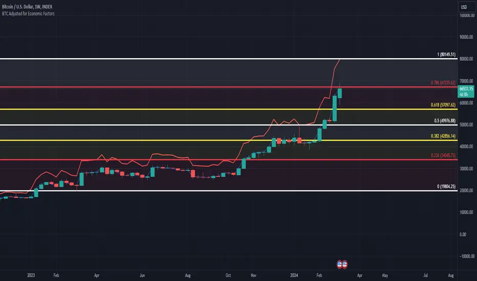
BTC/USD Inflation priced in! ~Period 2009 - 2023 (by TAS)The script creates a custom indicator titled "BTC Adjusted for Economic Factors.
Adjusted BTC Price is plotted in red, making it more prominent. The adjusted price is Bitcoin's historical closing prices adjusted for cumulative inflation over time, based on the Core Consumer Price Index (CPI) annual inflation rates from 2009 onwards.
The script calculates the adjusted price of Bitcoin by taking into account the effect of inflation on its value. It uses annual CPI rates for each year from 2009 to 2022 to calculate a cumulative inflation factor. The script assumes a placeholder inflation rate of 2.5% for 2023, indicating that this value should be updated when the actual rate is available. The script suggests adding CPI rates for additional years as they become available to maintain the accuracy of the adjustment.
Here's a breakdown of how the script works:
Core CPI Annual Inflation Rates: It starts by defining the annual inflation rates for each year from 2009 to 2022, expressed as a percentage divided by 100 to convert to a decimal.
Cumulative Inflation Calculation: The script calculates cumulative inflation starting from the year 2009 up to the current year. For each year that has passed since 2009, it multiplies the cumulative inflation factor by (1 + cpiRate), where cpiRate is the inflation rate for that year. This effectively compounds the inflation rate over time.
Adjusting Bitcoin's Price: The script then adjusts Bitcoin's closing price (close) for the calculated cumulative inflation to get the adjusted price (adjustedPrice).
Plotting the Prices: Finally, it plots both the original and the adjusted Bitcoin prices on the chart, allowing users to visually compare how inflation has theoretically impacted Bitcoin's value over time.
--------------------------------------------------------------------------------------------------
Important to notice, Fib. Retracements from the 2017 cycle top to the recent top (¬80K) doesn't look invalidated.
--------------------------------------------------------------------------------------------------
Inputs and feedback are welcome!
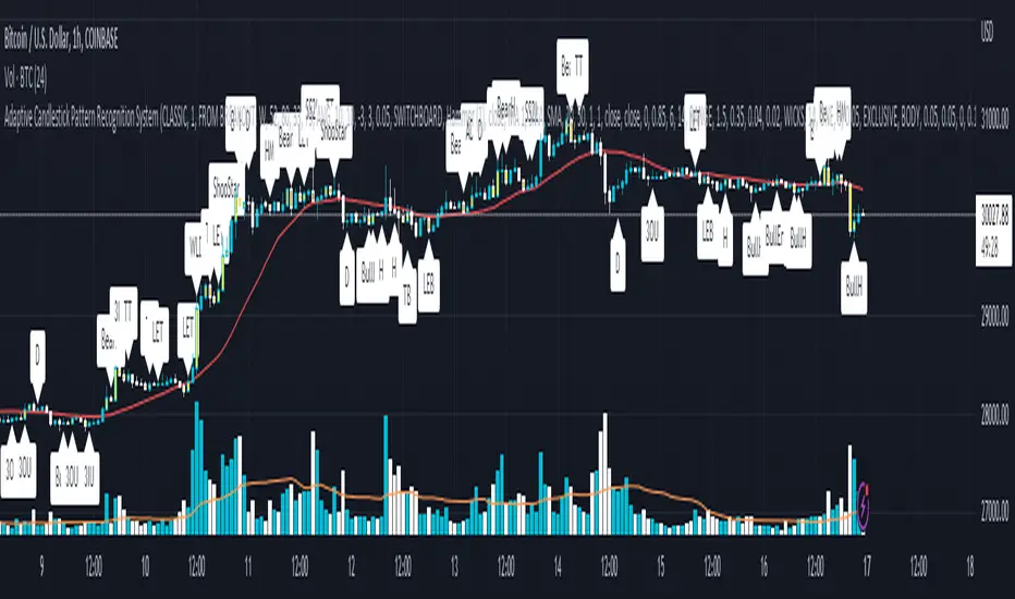
Adaptive Candlestick Pattern Recognition System█ INTRODUCTION
Nearly three years in the making, intermittently worked on in the few spare hours of weekends and time off, this is a passion project I undertook to flesh out my skills as a computer programmer. This script currently recognizes 85 different candlestick patterns ranging from one to five candles in length. It also performs statistical analysis on those patterns to determine prior performance and changes the coloration of those patterns based on that performance. In searching TradingView's script library for scripts similar to this one, I had found a handful. However, when I reviewed the ones which were open source, I did not see many that truly captured the power of PineScrypt or leveraged the way it works to create efficient and reliable code; one of the main driving factors for releasing this 5,000+ line behemoth open sourced.
Please take the time to review this description and source code to utilize this script to its fullest potential.
█ CONCEPTS
This script covers the following topics: Candlestick Theory, Trend Direction, Higher Timeframes, Price Analysis, Statistic Analysis, and Code Design.
Candlestick Theory - This script focuses solely on the concept of Candlestick Theory: arrangements of candlesticks may form certain patterns that can potentially influence the future price action of assets which experience those patterns. A full list of patterns (grouped by pattern length) will be in its own section of this description. This script contains two modes of operation for identifying candlestick patterns, 'CLASSIC' and 'BREAKOUT'.
CLASSIC: In this mode, candlestick patterns will be identified whenever they appear. The user has a wide variety of inputs to manipulate that can change how certain patterns are identified and even enable alerts to notify themselves when these patterns appear. Each pattern selected to appear will have their Profit or Loss (P/L) calculated starting from the first candle open succeeding the pattern to a candle close specified some number of candles ahead. These P/L calculations are then collected for each pattern, and split among partitions of prior price action of the asset the script is currently applied to (more on that in Higher Timeframes ).
BREAKOUT: In this mode, P/L calculations are held off until a breakout direction has been confirmed. The user may specify the number of candles ahead of a pattern's appearance (from one to five) that a pattern has to confirm a breakout in either an upward or downward direction. A breakout is constituted when there is a candle following the appearance of the pattern that closes above/at the highest high of the pattern, or below/at its lowest low. Only then will percent return calculations be performed for the pattern that's been identified, and these percent returns are broken up not only by the partition they had appeared in but also by the breakout direction itself. Patterns which do not breakout in either direction will be ignored, along with having their labels deleted.
In both of these modes, patterns may be overridden. Overrides occur when a smaller pattern has been detected and ends up becoming one (or more) of the candles of a larger pattern. A key example of this would be the Bearish Engulfing and the Three Outside Down patterns. A Three Outside Down necessitates a Bearish Engulfing as the first two candles in it, while the third candle closes lower. When a pattern is overridden, the return for that pattern will no longer be tracked. Overrides will not occur if the tail end of a larger pattern occurs at the beginning of a smaller pattern (Ex: a Bullish Engulfing occurs on the third candle of a Three Outside Down and the candle immediately following that pattern, the Three Outside Down pattern will not be overridden).
Important Functionality Note: These patterns are only searched for at the most recently closed candle, not on the currently closing candle, which creates an offset of one for this script's execution. (SEE LIMITATIONS)
Trend Direction - Many of the patterns require a trend direction prior to their appearance. Noting TradingView's own publication of candlestick patterns, I utilize a similar method for determining trend direction. Moving Averages are used to determine which trend is currently taking place for candlestick patterns to be sought out. The user has access to two Moving Averages which they may individually modify the following for each: Moving Average type (list of 9), their length, width, source values, and all variables associated with two special Moving Averages (Least Squares and Arnaud Legoux).
There are 3 settings for these Moving Averages, the first two switch between the two Moving Averages, and the third uses both. When using individual Moving Averages, the user may select a 'price point' to compare against the Moving Average (default is close). This price point is compared to the Moving Average at the candles prior to the appearance of candle patterns. Meaning: The close compared to the Moving Average two candles behind determines the trend direction used for Candlestick Analysis of one candle patterns; three candles behind for two candle patterns and so on. If the selected price point is above the Moving Average, then the current trend is an 'uptrend', 'downtrend' otherwise.
The third setting using both Moving Averages will compare the lengths of each, and trend direction is determined by the shorter Moving Average compared to the longer one. If the shorter Moving Average is above the longer, then the current trend is an 'uptrend', 'downtrend' otherwise. If the lengths of the Moving Averages are the same, or both Moving Averages are Symmetrical, then MA1 will be used by default. (SEE LIMITATIONS)
Higher Timeframes - This script employs the use of Higher Timeframes with a few request.security calls. The purpose of these calls is strictly for the partitioning of an asset's chart, splitting the returns of patterns into three separate groups. The four inputs in control of this partitioning split the chart based on: A given resolution to grab values from, the length of time in that resolution, and 'Upper' and 'Lower Limits' which split the trading range provided by that length of time in that resolution that forms three separate groups. The default values for these four inputs will partition the current chart by the yearly high-low range where: the 'Upper' partition is the top 20% of that trading range, the 'Middle' partition is 80% to 33% of the trading range, and the 'Lower' partition covers the trading range within 33% of the yearly low.
Patterns which are identified by this script will have their returns grouped together based on which partition they had appeared in. For example, a Bullish Engulfing which occurs within a third of the yearly low will have its return placed separately from a Bullish Engulfing that occurred within 20% of the yearly high. The idea is that certain patterns may perform better or worse depending on when they had occurred during an asset's trading range.
Price Analysis - Price Analysis is a major part of this script's functionality as it can fundamentally change how patterns are shown to the user. The settings related to Price Analysis include setting the number of candles ahead of a pattern's appearance to determine the return of that pattern. In 'BREAKOUT' mode, an additional setting allows the user to specify where the P/L calculation will begin for a pattern that had appeared and confirmed. (SEE LIMITATIONS)
The calculation for percent returns of patterns is illustrated with the following pseudo-code (CLASSIC mode, this is a simplified version of the actual code):
type patternObj
int ID
int partition
type returnsArray
float returns
// No pattern found = na returned
patternObj TEST_VAL = f_FindPattern()
priorTestVal = TEST_VAL
if not na( priorTestVal )
pnlMatrixRow = priorTestVal.ID
pnlMatrixCol = priorTestVal.partition
matrixReturn = matrix.get(PERCENT_RETURNS, pnlMatrixRow, pnlMatrixCol)
percentReturn = ( (close - open ) / open ) * 100%
array.push(matrixReturn.returns, percentReturn)
Statistic Analysis - This script uses Pine's built-in array functions to conduct the Statistic Analysis for patterns. When a pattern is found and its P/L calculation is complete, its return is added to a 'Return Array' User-Defined-Type that contains numerous fields which retain information on a pattern's prior performance. The actual UDT is as follows:
type returnArray
float returns = na
int size = 0
float avg = 0
float median = 0
float stdDev = 0
int polarities = na
All values within this UDT will be updated when a return is added to it (some based on user input). The array.avg , array.median and array.stdev will be ran and saved into their respective fields after a return is placed in the 'returns' array. The 'polarities' integer array is what will be changed based on user input. The user specifies two different percentages that declare 'Positive' and 'Negative' returns for patterns. When a pattern returns above, below, or in between these two values, different indices of this array will be incremented to reflect the kind of return that pattern had just experienced.
These values (plus the full name, partition the pattern occurred in, and a 95% confidence interval of expected returns) will be displayed to the user on the tooltip of the labels that identify patterns. Simply scroll over the pattern label to view each of these values.
Code Design - Overall this script is as much of an art piece as it is functional. Its design features numerous depictions of ASCII Art that illustrate what is being attempted by the functions that identify patterns, and an incalculable amount of time was spent rewriting portions of code to improve its efficiency. Admittedly, this final version is nearly 1,000 lines shorter than a previous version (one which took nearly 30 seconds after compilation to run, and didn't do nearly half of what this version does). The use of UDTs, especially the 'patternObj' one crafted and redesigned from the Hikkake Hunter 2.0 I published last month, played a significant role in making this script run efficiently. There is a slight rigidity in some of this code mainly around pattern IDs which are responsible for displaying the abbreviation for patterns (as well as the full names under the tooltips, and the matrix row position for holding returns), as each is hard-coded to correspond to that pattern.
However, one thing I would like to mention is the extensive use of global variables for pattern detection. Many scripts I had looked over for ideas on how to identify candlestick patterns had the same idea; break the pattern into a set of logical 'true/false' statements derived from historically referencing candle OHLC values. Some scripts which identified upwards of 20 to 30 patterns would reference Pine's built-in OHLC values for each pattern individually, potentially requesting information from TradingView's servers numerous times that could easily be saved into a variable for re-use and only requested once per candle (what this script does).
█ FEATURES
This script features a massive amount of switches, options, floating point values, detection settings, and methods for identifying/tailoring pattern appearances. All modifiable inputs for patterns are grouped together based on the number of candles they contain. Other inputs (like those for statistics settings and coloration) are grouped separately and presented in a way I believe makes the most sense.
Not mentioned above is the coloration settings. One of the aims of this script was to make patterns visually signify their behavior to the user when they are identified. Each pattern has its own collection of returns which are analyzed and compared to the inputs of the user. The user may choose the colors for bullish, neutral, and bearish patterns. They may also choose the minimum number of patterns needed to occur before assigning a color to that pattern based on its behavior; a color for patterns that have not met this minimum number of occurrences yet, and a color for patterns that are still processing in BREAKOUT mode.
There are also an additional three settings which alter the color scheme for patterns: Statistic Point-of-Reference, Adaptive coloring, and Hard Limiting. The Statistic Point-of-Reference decides which value (average or median) will be compared against the 'Negative' and 'Positive Return Tolerance'(s) to guide the coloration of the patterns (or for Adaptive Coloring, the generation of a color gradient).
Adaptive Coloring will have this script produce a gradient that patterns will be colored along. The more bullish or bearish a pattern is, the further along the gradient those patterns will be colored starting from the 'Neutral' color (hard lined at the value of 0%: values above this will be colored bullish, bearish otherwise). When Adaptive Coloring is enabled, this script will request the highest and lowest values (these being the Statistic Point-of-Reference) from the matrix containing all returns and rewrite global variables tied to the negative and positive return tolerances. This means that all patterns identified will be compared with each other to determine bullish/bearishness in Adaptive Coloring.
Hard Limiting will prevent these global variables from being rewritten, so patterns whose Statistic Point-of-Reference exceed the return tolerances will be fully colored the bullish or bearish colors instead of a generated gradient color. (SEE LIMITATIONS)
Apart from the Candle Detection Modes (CLASSIC and BREAKOUT), there's an additional two inputs which modify how this script behaves grouped under a "MASTER DETECTION SETTINGS" tab. These two "Pattern Detection Settings" are 'SWITCHBOARD' and 'TARGET MODE'.
SWITCHBOARD: Every single pattern has a switch that is associated with its detection. When a switch is enabled, the code which searches for that pattern will be run. With the Pattern Detection Setting set to this, all patterns that have their switches enabled will be sought out and shown.
TARGET MODE: There is an additional setting which operates on top of 'SWITCHBOARD' that singles out an individual pattern the user specifies through a drop down list. The names of every pattern recognized by this script will be present along with an identifier that shows the number of candles in that pattern (Ex: " (# candles)"). All patterns enabled in the switchboard will still have their returns measured, but only the pattern selected from the "Target Pattern" list will be shown. (SEE LIMITATIONS)
The vast majority of other features are held in the one, two, and three candle pattern sections.
For one-candle patterns, there are:
3 — Settings related to defining 'Tall' candles:
The number of candles to sample for previous candle-size averages.
The type of comparison done for 'Tall' Candles: Settings are 'RANGE' and 'BODY'.
The 'Tolerance' for tall candles, specifying what percent of the 'average' size candles must exceed to be considered 'Tall'.
When 'Tall Candle Setting' is set to RANGE, the high-low ranges are what the current candle range will be compared against to determine if a candle is 'Tall'. Otherwise the candle bodies (absolute value of the close - open) will be compared instead. (SEE LIMITATIONS)
Hammer Tolerance - How large a 'discarded wick' may be before it disqualifies a candle from being a 'Hammer'.
Discarded wicks are compared to the size of the Hammer's candle body and are dependent upon the body's center position. Hammer bodies closer to the high of the candle will have the upper wick used as its 'discarded wick', otherwise the lower wick is used.
9 — Doji Settings, some pulled from an old Doji Hunter I made a while back:
Doji Tolerance - How large the body of a candle may be compared to the range to be considered a 'Doji'.
Ignore N/S Dojis - Turns off Trend Direction for non-special Dojis.
GS/DF Doji Settings - 2 Inputs that enable and specify how large wicks that typically disqualify Dojis from being 'Gravestone' or 'Dragonfly' Dojis may be.
4 Settings related to 'Long Wick Doji' candles detailed below.
A Tolerance for 'Rickshaw Man' Dojis specifying how close the center of the body must be to the range to be valid.
The 4 settings the user may modify for 'Long Legged' Dojis are: A Sample Base for determining the previous average of wicks, a Sample Length specifying how far back to look for these averages, a Behavior Setting to define how 'Long Legged' Dojis are recognized, and a tolerance to specify how large in comparison to the prior wicks a Doji's wicks must be to be considered 'Long Legged'.
The 'Sample Base' list has two settings:
RANGE: The wicks of prior candles are compared to their candle ranges and the 'wick averages' will be what the average percent of ranges were in the sample.
WICKS: The size of the wicks themselves are averaged and returned for comparing against the current wicks of a Doji.
The 'Behavior' list has three settings:
ONE: Only one wick length needs to exceed the average by the tolerance for a Doji to be considered 'Long Legged'.
BOTH: Both wick lengths need to exceed the average of the tolerance of their respective wicks (upper wicks are compared to upper wicks, lower wicks compared to lower) to be considered 'Long Legged'.
AVG: Both wicks and the averages of the previous wicks are added together, divided by two, and compared. If the 'average' of the current wicks exceeds this combined average of prior wicks by the tolerance, then this would constitute a valid 'Long Legged' Doji. (For Dojis in general - SEE LIMITATIONS)
The final input is one related to candle patterns which require a Marubozu candle in them. The two settings for this input are 'INCLUSIVE' and 'EXCLUSIVE'. If INCLUSIVE is selected, any opening/closing variant of Marubozu candles will be allowed in the patterns that require them.
For two-candle patterns, there are:
2 — Settings which define 'Engulfing' parameters:
Engulfing Setting - Two options, RANGE or BODY which sets up how one candle may 'engulf' the previous.
Inclusive Engulfing - Boolean which enables if 'engulfing' candles can be equal to the values needed to 'engulf' the prior candle.
For the 'Engulfing Setting':
RANGE: If the second candle's high-low range completely covers the high-low range of the prior candle, this is recognized as 'engulfing'.
BODY: If the second candle's open-close completely covers the open-close of the previous candle, this is recognized as 'engulfing'. (SEE LIMITATIONS)
4 — Booleans specifying different settings for a few patterns:
One which allows for 'opens within body' patterns to let the second candle's open/close values match the prior candles' open/close.
One which forces 'Kicking' patterns to have a gap if the Marubozu setting is set to 'INCLUSIVE'.
And Two which dictate if the individual candles in 'Stomach' patterns need to be 'Tall'.
8 — Floating point values which affect 11 different patterns:
One which determines the distance the close of the first candle in a 'Hammer Inverted' pattern must be to the low to be considered valid.
One which affects how close the opens/closes need to be for all 'Lines' patterns (Bull/Bear Meeting/Separating Lines).
One that allows some leeway with the 'Matching Low' pattern (gives a small range the second candle close may be within instead of needing to match the previous close).
Three tolerances for On Neck/In Neck patterns (2 and 1 respectively).
A tolerance for the Thrusting pattern which give a range the close the second candle may be between the midpoint and close of the first to be considered 'valid'.
A tolerance for the two Tweezers patterns that specifies how close the highs and lows of the patterns need to be to each other to be 'valid'.
The first On Neck tolerance specifies how large the lower wick of the first candle may be (as a % of that candle's range) before the pattern is invalidated. The second tolerance specifies how far up the lower wick to the close the second candle's close may be for this pattern. The third tolerance for the In Neck pattern determines how far into the body of the first candle the second may close to be 'valid'.
For the remaining patterns (3, 4, and 5 candles), there are:
3 — Settings for the Deliberation pattern:
A boolean which forces the open of the third candle to gap above the close of the second.
A tolerance which changes the proximity of the third candle's open to the second candle's close in this pattern.
A tolerance that sets the maximum size the third candle may be compared to the average of the first two candles.
One boolean value for the Two Crows patterns (standard and Upside Gapping) that forces the first two candles in the patterns to completely gap if disabled (candle 1's close < candle 2's low).
10 — Floating point values for the remaining patterns:
One tolerance for defining how much the size of each candle in the Identical Black Crows pattern may deviate from the average of themselves to be considered valid.
One tolerance for setting how close the opens/closes of certain three candle patterns may be to each other's opens/closes.*
Three floating point values that affect the Three Stars in the South pattern.
One tolerance for the Side-by-Side patterns - looks at the second and third candle closes.
One tolerance for the Stick Sandwich pattern - looks at the first and third candle closes.
A floating value that sizes the Concealing Baby Swallow pattern's 3rd candle wick.
Two values for the Ladder Bottom pattern which define a range that the third candle's wick size may be.
* This affects the Three Black Crows (non-identical) and Three White Soldiers patterns, each require the opens and closes of every candle to be near each other.
The first tolerance of the Three Stars in the South pattern affects the first candle body's center position, and defines where it must be above to be considered valid. The second tolerance specifies how close the second candle must be to this same position, as well as the deviation the ratio the candle body to its range may be in comparison to the first candle. The third restricts how large the second candle range may be in comparison to the first (prevents this pattern from being recognized if the second candle is similar to the first but larger).
The last two floating point values define upper and lower limits to the wick size of a Ladder Bottom's fourth candle to be considered valid.
█ HOW TO USE
While there are many moving parts to this script, I attempted to set the default values with what I believed may help identify the most patterns within reasonable definitions. When this script is applied to a chart, the Candle Detection Mode (along with the BREAKOUT settings) and all candle switches must be confirmed before patterns are displayed. All switches are on by default, so this gives the user an opportunity to pick which patterns to identify first before playing around in the settings.
All of the settings/inputs described above are meant for experimentation. I encourage the user to tweak these values at will to find which set ups work best for whichever charts they decide to apply these patterns to.
Refer to the patterns themselves during experimentation. The statistic information provided on the tooltips of the patterns are meant to help guide input decisions. The breadth of candlestick theory is deep, and this was an attempt at capturing what I could in its sea of information.
█ LIMITATIONS
DISCLAIMER: While it may seem a bit paradoxical that this script aims to use past performance to potentially measure future results, past performance is not indicative of future results . Markets are highly adaptive and often unpredictable. This script is meant as an informational tool to show how patterns may behave. There is no guarantee that confidence intervals (or any other metric measured with this script) are accurate to the performance of patterns; caution must be exercised with all patterns identified regardless of how much information regarding prior performance is available.
Candlestick Theory - In the name, Candlestick Theory is a theory , and all theories come with their own limits. Some patterns identified by this script may be completely useless/unprofitable/unpredictable regardless of whatever combination of settings are used to identify them. However, if I truly believed this theory had no merit, this script would not exist. It is important to understand that this is a tool meant to be utilized with an array of others to procure positive (or negative, looking at you, short sellers ) results when navigating the complex world of finance.
To address the functionality note however, this script has an offset of 1 by default. Patterns will not be identified on the currently closing candle, only on the candle which has most recently closed. Attempting to have this script do both (offset by one or identify on close) lead to more trouble than it was worth. I personally just want users to be aware that patterns will not be identified immediately when they appear.
Trend Direction - Moving Averages - There is a small quirk with how MA settings will be adjusted if the user inputs two moving averages of the same length when the "MA Setting" is set to 'BOTH'. If Moving Averages have the same length, this script will default to only using MA 1 regardless of if the types of Moving Averages are different . I will experiment in the future to alleviate/reduce this restriction.
Price Analysis - BREAKOUT mode - With how identifying patterns with a look-ahead confirmation works, the percent returns for patterns that break out in either direction will be calculated on the same candle regardless of if P/L Offset is set to 'FROM CONFIRMATION' or 'FROM APPEARANCE'. This same issue is present in the Hikkake Hunter script mentioned earlier. This does not mean the P/L calculations are incorrect , the offset for the calculation is set by the number of candles required to confirm the pattern if 'FROM APPEARANCE' is selected. It just means that these two different P/L calculations will complete at the same time independent of the setting that's been selected.
Adaptive Coloring/Hard Limiting - Hard Limiting is only used with Adaptive Coloring and has no effect outside of it. If Hard Limiting is used, it is recommended to increase the 'Positive' and 'Negative' return tolerance values as a pattern's bullish/bearishness may be disproportionately represented with the gradient generated under a hard limit.
TARGET MODE - This mode will break rules regarding patterns that are overridden on purpose. If a pattern selected in TARGET mode would have otherwise been absorbed by a larger pattern, it will have that pattern's percent return calculated; potentially leading to duplicate returns being included in the matrix of all returns recognized by this script.
'Tall' Candle Setting - This is a wide-reaching setting, as approximately 30 different patterns or so rely on defining 'Tall' candles. Changing how 'Tall' candles are defined whether by the tolerance value those candles need to exceed or by the values of the candle used for the baseline comparison (RANGE/BODY) can wildly affect how this script functions under certain conditions. Refer to the tooltip of these settings for more information on which specific patterns are affected by this.
Doji Settings - There are roughly 10 or so two to three candle patterns which have Dojis as a part of them. If all Dojis are disabled, it will prevent some of these larger patterns from being recognized. This is a dependency issue that I may address in the future.
'Engulfing' Setting - Functionally, the two 'Engulfing' settings are quite different. Because of this, the 'RANGE' setting may cause certain patterns that would otherwise be valid under textbook and online references/definitions to not be recognized as such (like the Upside Gap Two Crows or Three Outside down).
█ PATTERN LIST
This script recognizes 85 patterns upon initial release. I am open to adding additional patterns to it in the future and any comments/suggestions are appreciated. It recognizes:
15 — 1 Candle Patterns
4 Hammer type patterns: Regular Hammer, Takuri Line, Shooting Star, and Hanging Man
9 Doji Candles: Regular Dojis, Northern/Southern Dojis, Gravestone/Dragonfly Dojis, Gapping Up/Down Dojis, and Long-Legged/Rickshaw Man Dojis
White/Black Long Days
32 — 2 Candle Patterns
4 Engulfing type patterns: Bullish/Bearish Engulfing and Last Engulfing Top/Bottom
Dark Cloud Cover
Bullish/Bearish Doji Star patterns
Hammer Inverted
Bullish/Bearish Haramis + Cross variants
Homing Pigeon
Bullish/Bearish Kicking
4 Lines type patterns: Bullish/Bearish Meeting/Separating Lines
Matching Low
On/In Neck patterns
Piercing pattern
Shooting Star (2 Lines)
Above/Below Stomach patterns
Thrusting
Tweezers Top/Bottom patterns
Two Black Gapping
Rising/Falling Window patterns
29 — 3 Candle Patterns
Bullish/Bearish Abandoned Baby patterns
Advance Block
Collapsing Doji Star
Deliberation
Upside/Downside Gap Three Methods patterns
Three Inside/Outside Up/Down patterns (4 total)
Bullish/Bearish Side-by-Side patterns
Morning/Evening Star patterns + Doji variants
Stick Sandwich
Downside/Upside Tasuki Gap patterns
Three Black Crows + Identical variation
Three White Soldiers
Three Stars in the South
Bullish/Bearish Tri-Star patterns
Two Crows + Upside Gap variant
Unique Three River Bottom
3 — 4 Candle Patterns
Concealing Baby Swallow
Bullish/Bearish Three Line Strike patterns
6 — 5 Candle Patterns
Bullish/Bearish Breakaway patterns
Ladder Bottom
Mat Hold
Rising/Falling Three Methods patterns
█ WORKS CITED
Because of the amount of time needed to complete this script, I am unable to provide exact dates for when some of these references were used. I will also not provide every single reference, as citing a reference for each individual pattern and the place it was reviewed would lead to a bibliography larger than this script and its description combined. There were five major resources I used when building this script, one book, two websites (for various different reasons including patterns, moving averages, and various other articles of information), various scripts from TradingView's public library (including TradingView's own source code for *all* candle patterns ), and PineScrypt's reference manual.
Bulkowski, Thomas N. Encyclopedia of Candlestick Patterns . Hoboken, New Jersey: John Wiley & Sons Inc., 2008. E-book (google books).
Various. Numerous webpages. CandleScanner . 2023. online. Accessed 2020 - 2023.
Various. Numerous webpages. Investopedia . 2023. online. Accessed 2020 - 2023.
█ AKNOWLEDGEMENTS
I want to take the time here to thank all of my friends and family, both online and in real life, for the support they've given me over the last few years in this endeavor. My pets who tried their hardest to keep me from completing it. And work for the grit to continue pushing through until this script's completion.
This belongs to me just as much as it does anyone else. Whether you are an institutional trader, gold bug hedging against the dollar, retail ape who got in on a squeeze, or just parents trying to grow their retirement/save for the kids. This belongs to everyone.
Private Beta for new features to be tested can be found here .
Vires In Numeris
Algoflow's Levels PlotterAlgoflow's Levels Plotter - Indicator
Release Date: Jan. 15, 2024
Release version: v3 r1
Release notes date: Jan. 15, 2024
Overview
Parses user's input of levels to be plotted and labeled on the chart for NQ & ES futures
Features
Quick plotting of predetermined price levels.
- Type or copy from another source of values in a predetermined output format.
Supports separate line plotting for Weekly, OVN and RTH values
- Plot only Weekly, OVN or RTH levels, or all
- Configure colors separately for Inflection Points, Weekly, OVN & RTH levels
- Shift/place price labels separately to easily identify levels
User Impacts of Changes
Requires users to remove previous version and re-add indicator "Algoflow's Levels Plotter", then re-add values. Colors and shift values will need to be re-entered and/or reconfigured
Support
Questions, feedbacks, and requests are welcomed. Please feel free to use Comments or direct private message via TradingView.
Quick usage notes:
The indicator allows you to enter data for both ES & NQ at the same time. This is useful in single chart window/layout situations, like viewing on the phone. When you switch between futures, the data is already there.
If you leave the entries blank, nothing will be plotted. This is useful if you want to have separate charts for ES & NQ. So you can just enter only the relevant data of either.
As an indicator, input values are saved within it, until it is removed from the chart. Input for one chart will not update other charts of the same ticker, even in the same layout.
The easiest and quickest way to share the inputs across all charts and layouts is to use the Indicator Templates feature.
- After input values are entered (for both ES & NQ futures) via the indicator's Settings, select ""Save as Default"".
- Click on ""Indicator Templates"" (4 squares icon), and click on ""Save Indicator template...""
- Remove the previous version of the indicator in other charts.
- Click on ""Indicator Templates"" icon, and select the newly created template. Repeat this for other charts of the same futures ticker
The labels can be disabled in settings > Style tab. Use the Inputs tab to configure orientation (left or right of current bar on chart), and how much spacing from the current (in distance of bars)
Format example:
Primary directional inflection point: 1234
For Bulls: 1244.25, 1254, 1264.50
For Bears: 1224, 1214, 1204
Changes
v3 r1 - Fixed erroneous default values in Weekly input sections. Added options to en/disable display of each set (session) of levels. Default label text size to normal, from small.
- Jan 15, 2024
v2 r9 - Added support for USTEC & US500.
- Dec. 10, 2023
v2 r8 - Added configuration features for users to modify the labels' text colors and size. Simplified code further by moving inputs processing modules into a single user function.
- Oct. 31, 2023
v2 r7 - Added support for the micro NQ & ES. Modified to ignore string case in inputs
- Oct 18, 2023
v2 r4 - Added support of weekly lines and labels features. Began the process of optimizing/simplifying code
- Oct. 15, 2023
v2 r3 - Made Inflection Point levels' colors configurable
- Oct. 04, 2023
v2 r2 - Removed comments & debug codes from development build revision #518
- Oct. 04, 2023
v2 r1 - Released from development revision #518. Major rewrite to fix previous and overlapping plots of lines and labels.
- Oct. 04, 2023
v1 r2 - First release of indicator
- Oct. 02, 2023

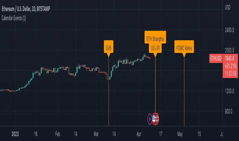
Economic Calendar EventsThis indicator provides an overlay of Events on the main chart, where each Event is visually represented by a Label and vertical Line, placed at the specified time interval for each Event.
Events are defined by user data as an input string on the settings widget panel for the indicator. The event data is a string (semicolon delimited) whose grammar is a representation of a collection of Event records, where each Event record is a comma-separated list of fields, which correspond to:
The name of the event.
The symbol or ticker to which the Event applies (or `*` if it should apply to all ticklers).
The timezone and then the year, month, day, hour, and minute of the event, respectively.
Each Event record is separated by the semicolon ";" character.
As an example , assume `evantData` is the string:
"SVB,*,UTC,2023,03,10,00,00;US CPI,*,UTC,2023,04,12,08,30;ETH Shanghai,ETHUSD,UTC,2023,04,12,08,30"
In the above case, there are 4 Events defined, three of which apply to all tickers and one applies only to ETHUSD, as follows:
The first event is named SVB and applies to all tickers at UTC time on March 10, 2023 at 12:00:00.
The second event is named US CPI and applies to all tickers at UTC time on April 12, 2023 at 08:30:00.
The third event is named ETH Shanghai and applies to the ETHUSD ticker at UTC time on April 12, 2023 at 08:30:00.
The fourth event is named FOMC Rates and applies to all tickers at UTC time on May 3, 2023 at 14:00:00.
The following is a BNF for defining event data:
market-events ::= event-record | event-record ";" market-events
event-record ::= event-name "," ticker ”,” event-timezone "," event-time
event-name ::= string
event-time>::= year "," month "," day "," hour "," minute
event-timezone ::= string
ticker ::= "*" | string
string ::= +
year ::= {4}
month ::= {2}
day ::= {2}
hour ::= {2}
minute ::= {2}
Ray Dalio's All Weather Strategy - Portfolio CalculatorTHE ALL WEATHER STRATEGY INDICATOR: A GUIDE TO RAY DALIO'S LEGENDARY PORTFOLIO APPROACH
Introduction: The Genesis of Financial Resilience
In the sprawling corridors of Bridgewater Associates, the world's largest hedge fund managing over 150 billion dollars in assets, Ray Dalio conceived what would become one of the most influential investment strategies of the modern era. The All Weather Strategy, born from decades of market observation and rigorous backtesting, represents a paradigm shift from traditional portfolio construction methods that have dominated Wall Street since Harry Markowitz's seminal work on Modern Portfolio Theory in 1952.
Unlike conventional approaches that chase returns through market timing or stock picking, the All Weather Strategy embraces a fundamental truth that has humbled countless investors throughout history: nobody can consistently predict the future direction of markets. Instead of fighting this uncertainty, Dalio's approach harnesses it, creating a portfolio designed to perform reasonably well across all economic environments, hence the evocative name "All Weather."
The strategy emerged from Bridgewater's extensive research into economic cycles and asset class behavior, culminating in what Dalio describes as "the Holy Grail of investing" in his bestselling book "Principles" (Dalio, 2017). This Holy Grail isn't about achieving spectacular returns, but rather about achieving consistent, risk-adjusted returns that compound steadily over time, much like the tortoise defeating the hare in Aesop's timeless fable.
HISTORICAL DEVELOPMENT AND EVOLUTION
The All Weather Strategy's origins trace back to the tumultuous economic periods of the 1970s and 1980s, when traditional portfolio construction methods proved inadequate for navigating simultaneous inflation and recession. Raymond Thomas Dalio, born in 1949 in Queens, New York, founded Bridgewater Associates from his Manhattan apartment in 1975, initially focusing on currency and fixed-income consulting for corporate clients.
Dalio's early experiences during the 1970s stagflation period profoundly shaped his investment philosophy. Unlike many of his contemporaries who viewed inflation and deflation as opposing forces, Dalio recognized that both conditions could coexist with either economic growth or contraction, creating four distinct economic environments rather than the traditional two-factor models that dominated academic finance.
The conceptual breakthrough came in the late 1980s when Dalio began systematically analyzing asset class performance across different economic regimes. Working with a small team of researchers, Bridgewater developed sophisticated models that decomposed economic conditions into growth and inflation components, then mapped historical asset class returns against these regimes. This research revealed that traditional portfolio construction, heavily weighted toward stocks and bonds, left investors vulnerable to specific economic scenarios.
The formal All Weather Strategy emerged in 1996 when Bridgewater was approached by a wealthy family seeking a portfolio that could protect their wealth across various economic conditions without requiring active management or market timing. Unlike Bridgewater's flagship Pure Alpha fund, which relied on active trading and leverage, the All Weather approach needed to be completely passive and unleveraged while still providing adequate diversification.
Dalio and his team spent months developing and testing various allocation schemes, ultimately settling on the 30/40/15/7.5/7.5 framework that balances risk contributions rather than dollar amounts. This approach was revolutionary because it focused on risk budgeting—ensuring that no single asset class dominated the portfolio's risk profile—rather than the traditional approach of equal dollar allocations or market-cap weighting.
The strategy's first institutional implementation began in 1996 with a family office client, followed by gradual expansion to other wealthy families and eventually institutional investors. By 2005, Bridgewater was managing over $15 billion in All Weather assets, making it one of the largest systematic strategy implementations in institutional investing.
The 2008 financial crisis provided the ultimate test of the All Weather methodology. While the S&P 500 declined by 37% and many hedge funds suffered double-digit losses, the All Weather strategy generated positive returns, validating Dalio's risk-balancing approach. This performance during extreme market stress attracted significant institutional attention, leading to rapid asset growth in subsequent years.
The strategy's theoretical foundations evolved throughout the 2000s as Bridgewater's research team, led by co-chief investment officers Greg Jensen and Bob Prince, refined the economic framework and incorporated insights from behavioral economics and complexity theory. Their research, published in numerous institutional white papers, demonstrated that traditional portfolio optimization methods consistently underperformed simpler risk-balanced approaches across various time periods and market conditions.
Academic validation came through partnerships with leading business schools and collaboration with prominent economists. The strategy's risk parity principles influenced an entire generation of institutional investors, leading to the creation of numerous risk parity funds managing hundreds of billions in aggregate assets.
In recent years, the democratization of sophisticated financial tools has made All Weather-style investing accessible to individual investors through ETFs and systematic platforms. The availability of high-quality, low-cost ETFs covering each required asset class has eliminated many of the barriers that previously limited sophisticated portfolio construction to institutional investors.
The development of advanced portfolio management software and platforms like TradingView has further democratized access to institutional-quality analytics and implementation tools. The All Weather Strategy Indicator represents the culmination of this trend, providing individual investors with capabilities that previously required teams of portfolio managers and risk analysts.
Understanding the Four Economic Seasons
The All Weather Strategy's theoretical foundation rests on Dalio's observation that all economic environments can be characterized by two primary variables: economic growth and inflation. These variables create four distinct "economic seasons," each favoring different asset classes. Rising growth benefits stocks and commodities, while falling growth favors bonds. Rising inflation helps commodities and inflation-protected securities, while falling inflation benefits nominal bonds and stocks.
This framework, detailed extensively in Bridgewater's research papers from the 1990s, suggests that by holding assets that perform well in each economic season, an investor can create a portfolio that remains resilient regardless of which season unfolds. The elegance lies not in predicting which season will occur, but in being prepared for all of them simultaneously.
Academic research supports this multi-environment approach. Ang and Bekaert (2002) demonstrated that regime changes in economic conditions significantly impact asset returns, while Fama and French (2004) showed that different asset classes exhibit varying sensitivities to economic factors. The All Weather Strategy essentially operationalizes these academic insights into a practical investment framework.
The Original All Weather Allocation: Simplicity Masquerading as Sophistication
The core All Weather portfolio, as implemented by Bridgewater for institutional clients and later adapted for retail investors, maintains a deceptively simple static allocation: 30% stocks, 40% long-term bonds, 15% intermediate-term bonds, 7.5% commodities, and 7.5% Treasury Inflation-Protected Securities (TIPS). This allocation may appear arbitrary to the uninitiated, but each percentage reflects careful consideration of historical volatilities, correlations, and economic sensitivities.
The 30% stock allocation provides growth exposure while limiting the portfolio's overall volatility. Stocks historically deliver superior long-term returns but with significant volatility, as evidenced by the Standard & Poor's 500 Index's average annual return of approximately 10% since 1926, accompanied by standard deviation exceeding 15% (Ibbotson Associates, 2023). By limiting stock exposure to 30%, the portfolio captures much of the equity risk premium while avoiding excessive volatility.
The combined 55% allocation to bonds (40% long-term plus 15% intermediate-term) serves as the portfolio's stabilizing force. Long-term bonds provide substantial interest rate sensitivity, performing well during economic slowdowns when central banks reduce rates. Intermediate-term bonds offer a balance between interest rate sensitivity and reduced duration risk. This bond-heavy allocation reflects Dalio's insight that bonds typically exhibit lower volatility than stocks while providing essential diversification benefits.
The 7.5% commodities allocation addresses inflation protection, as commodity prices typically rise during inflationary periods. Historical analysis by Bodie and Rosansky (1980) demonstrated that commodities provide meaningful diversification benefits and inflation hedging capabilities, though with considerable volatility. The relatively small allocation reflects commodities' high volatility and mixed long-term returns.
Finally, the 7.5% TIPS allocation provides explicit inflation protection through government-backed securities whose principal and interest payments adjust with inflation. Introduced by the U.S. Treasury in 1997, TIPS have proven effective inflation hedges, though they underperform nominal bonds during deflationary periods (Campbell & Viceira, 2001).
Historical Performance: The Evidence Speaks
Analyzing the All Weather Strategy's historical performance reveals both its strengths and limitations. Using monthly return data from 1970 to 2023, spanning over five decades of varying economic conditions, the strategy has delivered compelling risk-adjusted returns while experiencing lower volatility than traditional stock-heavy portfolios.
During this period, the All Weather allocation generated an average annual return of approximately 8.2%, compared to 10.5% for the S&P 500 Index. However, the strategy's annual volatility measured just 9.1%, substantially lower than the S&P 500's 15.8% volatility. This translated to a Sharpe ratio of 0.67 for the All Weather Strategy versus 0.54 for the S&P 500, indicating superior risk-adjusted performance.
More impressively, the strategy's maximum drawdown over this period was 12.3%, occurring during the 2008 financial crisis, compared to the S&P 500's maximum drawdown of 50.9% during the same period. This drawdown mitigation proves crucial for long-term wealth building, as Stein and DeMuth (2003) demonstrated that avoiding large losses significantly impacts compound returns over time.
The strategy performed particularly well during periods of economic stress. During the 1970s stagflation, when stocks and bonds both struggled, the All Weather portfolio's commodity and TIPS allocations provided essential protection. Similarly, during the 2000-2002 dot-com crash and the 2008 financial crisis, the portfolio's bond-heavy allocation cushioned losses while maintaining positive returns in several years when stocks declined significantly.
However, the strategy underperformed during sustained bull markets, particularly the 1990s technology boom and the 2010s post-financial crisis recovery. This underperformance reflects the strategy's conservative nature and diversified approach, which sacrifices potential upside for downside protection. As Dalio frequently emphasizes, the All Weather Strategy prioritizes "not losing money" over "making a lot of money."
Implementing the All Weather Strategy: A Practical Guide
The All Weather Strategy Indicator transforms Dalio's institutional-grade approach into an accessible tool for individual investors. The indicator provides real-time portfolio tracking, rebalancing signals, and performance analytics, eliminating much of the complexity traditionally associated with implementing sophisticated allocation strategies.
To begin implementation, investors must first determine their investable capital. As detailed analysis reveals, the All Weather Strategy requires meaningful capital to implement effectively due to transaction costs, minimum investment requirements, and the need for precise allocations across five different asset classes.
For portfolios below $50,000, the strategy becomes challenging to implement efficiently. Transaction costs consume a disproportionate share of returns, while the inability to purchase fractional shares creates allocation drift. Consider an investor with $25,000 attempting to allocate 7.5% to commodities through the iPath Bloomberg Commodity Index ETF (DJP), currently trading around $25 per share. This allocation targets $1,875, enough for only 75 shares, creating immediate tracking error.
At $50,000, implementation becomes feasible but not optimal. The 30% stock allocation ($15,000) purchases approximately 37 shares of the SPDR S&P 500 ETF (SPY) at current prices around $400 per share. The 40% long-term bond allocation ($20,000) buys 200 shares of the iShares 20+ Year Treasury Bond ETF (TLT) at approximately $100 per share. While workable, these allocations leave significant cash drag and rebalancing challenges.
The optimal minimum for individual implementation appears to be $100,000. At this level, each allocation becomes substantial enough for precise implementation while keeping transaction costs below 0.4% annually. The $30,000 stock allocation, $40,000 long-term bond allocation, $15,000 intermediate-term bond allocation, $7,500 commodity allocation, and $7,500 TIPS allocation each provide sufficient size for effective management.
For investors with $250,000 or more, the strategy implementation approaches institutional quality. Allocation precision improves, transaction costs decline as a percentage of assets, and rebalancing becomes highly efficient. These larger portfolios can also consider adding complexity through international diversification or alternative implementations.
The indicator recommends quarterly rebalancing to balance transaction costs with allocation discipline. Monthly rebalancing increases costs without substantial benefits for most investors, while annual rebalancing allows excessive drift that can meaningfully impact performance. Quarterly rebalancing, typically on the first trading day of each quarter, provides an optimal balance.
Understanding the Indicator's Functionality
The All Weather Strategy Indicator operates as a comprehensive portfolio management system, providing multiple analytical layers that professional money managers typically reserve for institutional clients. This sophisticated tool transforms Ray Dalio's institutional-grade strategy into an accessible platform for individual investors, offering features that rival professional portfolio management software.
The indicator's core architecture consists of several interconnected modules that work seamlessly together to provide complete portfolio oversight. At its foundation lies a real-time portfolio simulation engine that tracks the exact value of each ETF position based on current market prices, eliminating the need for manual calculations or external spreadsheets.
DETAILED INDICATOR COMPONENTS AND FUNCTIONS
Portfolio Configuration Module
The portfolio setup begins with the Portfolio Configuration section, which establishes the fundamental parameters for strategy implementation. The Portfolio Capital input accepts values from $1,000 to $10,000,000, accommodating everyone from beginning investors to institutional clients. This input directly drives all subsequent calculations, determining exact share quantities and portfolio values throughout the implementation period.
The Portfolio Start Date function allows users to specify when they began implementing the All Weather Strategy, creating a clear demarcation point for performance tracking. This feature proves essential for investors who want to track their actual implementation against theoretical performance, providing realistic assessment of strategy effectiveness including timing differences and implementation costs.
Rebalancing Frequency settings offer two options: Monthly and Quarterly. While monthly rebalancing provides more precise allocation control, quarterly rebalancing typically proves more cost-effective for most investors due to reduced transaction costs. The indicator automatically detects the first trading day of each period, ensuring rebalancing occurs at optimal times regardless of weekends, holidays, or market closures.
The Rebalancing Threshold parameter, adjustable from 0.5% to 10%, determines when allocation drift triggers rebalancing recommendations. Conservative settings like 1-2% maintain tight allocation control but increase trading frequency, while wider thresholds like 3-5% reduce trading costs but allow greater allocation drift. This flexibility accommodates different risk tolerances and cost structures.
Visual Display System
The Show All Weather Calculator toggle controls the main dashboard visibility, allowing users to focus on chart visualization when detailed metrics aren't needed. When enabled, this comprehensive dashboard displays current portfolio value, individual ETF allocations, target versus actual weights, rebalancing status, and performance metrics in a professionally formatted table.
Economic Environment Display provides context about current market conditions based on growth and inflation indicators. While simplified compared to Bridgewater's sophisticated regime detection, this feature helps users understand which economic "season" currently prevails and which asset classes should theoretically benefit.
Rebalancing Signals illuminate when portfolio drift exceeds user-defined thresholds, highlighting specific ETFs that require adjustment. These signals use color coding to indicate urgency: green for balanced allocations, yellow for moderate drift, and red for significant deviations requiring immediate attention.
Advanced Label System
The rebalancing label system represents one of the indicator's most innovative features, providing three distinct detail levels to accommodate different user needs and experience levels. The "None" setting displays simple symbols marking portfolio start and rebalancing events without cluttering the chart with text. This minimal approach suits experienced investors who understand the implications of each symbol.
"Basic" label mode shows essential information including portfolio values at each rebalancing point, enabling quick assessment of strategy performance over time. These labels display "START $X" for portfolio initiation and "RBL $Y" for rebalancing events, providing clear performance tracking without overwhelming detail.
"Detailed" labels provide comprehensive trading instructions including exact buy and sell quantities for each ETF. These labels might display "RBL $125,000 BUY 15 SPY SELL 25 TLT BUY 8 IEF NO TRADES DJP SELL 12 SCHP" providing complete implementation guidance. This feature essentially transforms the indicator into a personal portfolio manager, eliminating guesswork about exact trades required.
Professional Color Themes
Eight professionally designed color themes adapt the indicator's appearance to different aesthetic preferences and market analysis styles. The "Gold" theme reflects traditional wealth management aesthetics, while "EdgeTools" provides modern professional appearance. "Behavioral" uses psychologically informed colors that reinforce disciplined decision-making, while "Quant" employs high-contrast combinations favored by quantitative analysts.
"Ocean," "Fire," "Matrix," and "Arctic" themes provide distinctive visual identities for traders who prefer unique chart aesthetics. Each theme automatically adjusts for dark or light mode optimization, ensuring optimal readability across different TradingView configurations.
Real-Time Portfolio Tracking
The portfolio simulation engine continuously tracks five separate ETF positions: SPY for stocks, TLT for long-term bonds, IEF for intermediate-term bonds, DJP for commodities, and SCHP for TIPS. Each position's value updates in real-time based on current market prices, providing instant feedback about portfolio performance and allocation drift.
Current share calculations determine exact holdings based on the most recent rebalancing, while target shares reflect optimal allocation based on current portfolio value. Trade calculations show precisely how many shares to buy or sell during rebalancing, eliminating manual calculations and potential errors.
Performance Analytics Suite
The indicator's performance measurement capabilities rival professional portfolio analysis software. Sharpe ratio calculations incorporate current risk-free rates obtained from Treasury yield data, providing accurate risk-adjusted performance assessment. Volatility measurements use rolling periods to capture changing market conditions while maintaining statistical significance.
Portfolio return calculations track both absolute and relative performance, comparing the All Weather implementation against individual asset classes and benchmark indices. These metrics update continuously, providing real-time assessment of strategy effectiveness and implementation quality.
Data Quality Monitoring
Sophisticated data quality checks ensure reliable indicator operation across different market conditions and potential data interruptions. The system monitors all five ETF price feeds plus economic data sources, providing quality scores that alert users to potential data issues that might affect calculations.
When data quality degrades, the indicator automatically switches to fallback values or alternative data sources, maintaining functionality during temporary market data interruptions. This robust design ensures consistent operation even during volatile market conditions when data feeds occasionally experience disruptions.
Risk Management and Behavioral Considerations
Despite its sophisticated design, the All Weather Strategy faces behavioral challenges that have derailed countless well-intentioned investment plans. The strategy's conservative nature means it will underperform growth stocks during bull markets, potentially by substantial margins. Maintaining discipline during these periods requires understanding that the strategy optimizes for risk-adjusted returns over absolute returns.
Behavioral finance research by Kahneman and Tversky (1979) demonstrates that investors feel losses approximately twice as intensely as equivalent gains. This loss aversion creates powerful psychological pressure to abandon defensive strategies during bull markets when aggressive portfolios appear more attractive. The All Weather Strategy's bond-heavy allocation will seem overly conservative when technology stocks double in value, as occurred repeatedly during the 2010s.
Conversely, the strategy's defensive characteristics provide psychological comfort during market stress. When stocks crash 30-50%, as they periodically do, the All Weather portfolio's modest losses feel manageable rather than catastrophic. This emotional stability enables investors to maintain their investment discipline when others capitulate, often at the worst possible times.
Rebalancing discipline presents another behavioral challenge. Selling winners to buy losers contradicts natural human tendencies but remains essential for the strategy's success. When stocks have outperformed bonds for several quarters, rebalancing requires selling high-performing stock positions to purchase seemingly stagnant bond positions. This action feels counterintuitive but captures the strategy's systematic approach to risk management.
Tax considerations add complexity for taxable accounts. Frequent rebalancing generates taxable events that can erode after-tax returns, particularly for high-income investors facing elevated capital gains rates. Tax-advantaged accounts like 401(k)s and IRAs provide ideal vehicles for All Weather implementation, eliminating tax friction from rebalancing activities.
Capital Requirements and Cost Analysis
Comprehensive cost analysis reveals the capital requirements for effective All Weather implementation. Annual expenses include management fees for each ETF, transaction costs from rebalancing, and bid-ask spreads from trading less liquid securities.
ETF expense ratios vary significantly across asset classes. The SPDR S&P 500 ETF charges 0.09% annually, while the iShares 20+ Year Treasury Bond ETF charges 0.20%. The iShares 7-10 Year Treasury Bond ETF charges 0.15%, the Schwab US TIPS ETF charges 0.05%, and the iPath Bloomberg Commodity Index ETF charges 0.75%. Weighted by the All Weather allocations, total expense ratios average approximately 0.19% annually.
Transaction costs depend heavily on broker selection and account size. Premium brokers like Interactive Brokers charge $1-2 per trade, resulting in $20-40 annually for quarterly rebalancing. Discount brokers may charge higher per-trade fees but offer commission-free ETF trading for selected funds. Zero-commission brokers eliminate explicit trading costs but often impose wider bid-ask spreads that function as hidden fees.
Bid-ask spreads represent the difference between buying and selling prices for each security. Highly liquid ETFs like SPY maintain spreads of 1-2 basis points, while less liquid commodity ETFs may exhibit spreads of 5-10 basis points. These costs accumulate through rebalancing activities, typically totaling 10-15 basis points annually.
For a $100,000 portfolio, total annual costs including expense ratios, transaction fees, and spreads typically range from 0.35% to 0.45%, or $350-450 annually. These costs decline as a percentage of assets as portfolio size increases, reaching approximately 0.25% for portfolios exceeding $250,000.
Comparing costs to potential benefits reveals the strategy's value proposition. Historical analysis suggests the All Weather approach reduces portfolio volatility by 35-40% compared to stock-heavy allocations while maintaining competitive returns. This volatility reduction provides substantial value during market stress, potentially preventing behavioral mistakes that destroy long-term wealth.
Alternative Implementations and Customizations
While the original All Weather allocation provides an excellent starting point, investors may consider modifications based on personal circumstances, market conditions, or geographic considerations. International diversification represents one potential enhancement, adding exposure to developed and emerging market bonds and equities.
Geographic customization becomes important for non-US investors. European investors might replace US Treasury bonds with German Bunds or broader European government bond indices. Currency hedging decisions add complexity but may reduce volatility for investors whose spending occurs in non-dollar currencies.
Tax-location strategies optimize after-tax returns by placing tax-inefficient assets in tax-advantaged accounts while holding tax-efficient assets in taxable accounts. TIPS and commodity ETFs generate ordinary income taxed at higher rates, making them candidates for retirement account placement. Stock ETFs generate qualified dividends and long-term capital gains taxed at lower rates, making them suitable for taxable accounts.
Some investors prefer implementing the bond allocation through individual Treasury securities rather than ETFs, eliminating management fees while gaining precise maturity control. Treasury auctions provide access to new securities without bid-ask spreads, though this approach requires more sophisticated portfolio management.
Factor-based implementations replace broad market ETFs with factor-tilted alternatives. Value-tilted stock ETFs, quality-focused bond ETFs, or momentum-based commodity indices may enhance returns while maintaining the All Weather framework's diversification benefits. However, these modifications introduce additional complexity and potential tracking error.
Conclusion: Embracing the Long Game
The All Weather Strategy represents more than an investment approach; it embodies a philosophy of financial resilience that prioritizes sustainable wealth building over speculative gains. In an investment landscape increasingly dominated by algorithmic trading, meme stocks, and cryptocurrency volatility, Dalio's methodical approach offers a refreshing alternative grounded in economic theory and historical evidence.
The strategy's greatest strength lies not in its potential for extraordinary returns, but in its capacity to deliver reasonable returns across diverse economic environments while protecting capital during market stress. This characteristic becomes increasingly valuable as investors approach or enter retirement, when portfolio preservation assumes greater importance than aggressive growth.
Implementation requires discipline, adequate capital, and realistic expectations. The strategy will underperform growth-oriented approaches during bull markets while providing superior downside protection during bear markets. Investors must embrace this trade-off consciously, understanding that the strategy optimizes for long-term wealth building rather than short-term performance.
The All Weather Strategy Indicator democratizes access to institutional-quality portfolio management, providing individual investors with tools previously available only to wealthy families and institutions. By automating allocation tracking, rebalancing signals, and performance analysis, the indicator removes much of the complexity that has historically limited sophisticated strategy implementation.
For investors seeking a systematic, evidence-based approach to long-term wealth building, the All Weather Strategy provides a compelling framework. Its emphasis on diversification, risk management, and behavioral discipline aligns with the fundamental principles that have created lasting wealth throughout financial history. While the strategy may not generate headlines or inspire cocktail party conversations, it offers something more valuable: a reliable path toward financial security across all economic seasons.
As Dalio himself notes, "The biggest mistake investors make is to believe that what happened in the recent past is likely to persist, and they design their portfolios accordingly." The All Weather Strategy's enduring appeal lies in its rejection of this recency bias, instead embracing the uncertainty of markets while positioning for success regardless of which economic season unfolds.
STEP-BY-STEP INDICATOR SETUP GUIDE
Setting up the All Weather Strategy Indicator requires careful attention to each configuration parameter to ensure optimal implementation. This comprehensive setup guide walks through every setting and explains its impact on strategy performance.
Initial Setup Process
Begin by adding the indicator to your TradingView chart. Search for "Ray Dalio's All Weather Strategy" in the indicator library and apply it to any chart. The indicator operates independently of the underlying chart symbol, drawing data directly from the five required ETFs regardless of which security appears on the chart.
Portfolio Configuration Settings
Start with the Portfolio Capital input, which drives all subsequent calculations. Enter your exact investable capital, ranging from $1,000 to $10,000,000. This input determines share quantities, trade recommendations, and performance calculations. Conservative recommendations suggest minimum capitals of $50,000 for basic implementation or $100,000 for optimal precision.
Select your Portfolio Start Date carefully, as this establishes the baseline for all performance calculations. Choose the date when you actually began implementing the All Weather Strategy, not when you first learned about it. This date should reflect when you first purchased ETFs according to the target allocation, creating realistic performance tracking.
Choose your Rebalancing Frequency based on your cost structure and precision preferences. Monthly rebalancing provides tighter allocation control but increases transaction costs. Quarterly rebalancing offers the optimal balance for most investors between allocation precision and cost control. The indicator automatically detects appropriate trading days regardless of your selection.
Set the Rebalancing Threshold based on your tolerance for allocation drift and transaction costs. Conservative investors preferring tight control should use 1-2% thresholds, while cost-conscious investors may prefer 3-5% thresholds. Lower thresholds maintain more precise allocations but trigger more frequent trading.
Display Configuration Options
Enable Show All Weather Calculator to display the comprehensive dashboard containing portfolio values, allocations, and performance metrics. This dashboard provides essential information for portfolio management and should remain enabled for most users.
Show Economic Environment displays current economic regime classification based on growth and inflation indicators. While simplified compared to Bridgewater's sophisticated models, this feature provides useful context for understanding current market conditions.
Show Rebalancing Signals highlights when portfolio allocations drift beyond your threshold settings. These signals use color coding to indicate urgency levels, helping prioritize rebalancing activities.
Advanced Label Customization
Configure Show Rebalancing Labels based on your need for chart annotations. These labels mark important portfolio events and can provide valuable historical context, though they may clutter charts during extended time periods.
Select appropriate Label Detail Levels based on your experience and information needs. "None" provides minimal symbols suitable for experienced users. "Basic" shows portfolio values at key events. "Detailed" provides complete trading instructions including exact share quantities for each ETF.
Appearance Customization
Choose Color Themes based on your aesthetic preferences and trading style. "Gold" reflects traditional wealth management appearance, while "EdgeTools" provides modern professional styling. "Behavioral" uses psychologically informed colors that reinforce disciplined decision-making.
Enable Dark Mode Optimization if using TradingView's dark theme for optimal readability and contrast. This setting automatically adjusts all colors and transparency levels for the selected theme.
Set Main Line Width based on your chart resolution and visual preferences. Higher width values provide clearer allocation lines but may overwhelm smaller charts. Most users prefer width settings of 2-3 for optimal visibility.
Troubleshooting Common Setup Issues
If the indicator displays "Data not available" messages, verify that all five ETFs (SPY, TLT, IEF, DJP, SCHP) have valid price data on your selected timeframe. The indicator requires daily data availability for all components.
When rebalancing signals seem inconsistent, check your threshold settings and ensure sufficient time has passed since the last rebalancing event. The indicator only triggers signals on designated rebalancing days (first trading day of each period) when drift exceeds threshold levels.
If labels appear at unexpected chart locations, verify that your chart displays percentage values rather than price values. The indicator forces percentage formatting and 0-40% scaling for optimal allocation visualization.
COMPREHENSIVE BIBLIOGRAPHY AND FURTHER READING
PRIMARY SOURCES AND RAY DALIO WORKS
Dalio, R. (2017). Principles: Life and work. New York: Simon & Schuster.
Dalio, R. (2018). A template for understanding big debt crises. Bridgewater Associates.
Dalio, R. (2021). Principles for dealing with the changing world order: Why nations succeed and fail. New York: Simon & Schuster.
BRIDGEWATER ASSOCIATES RESEARCH PAPERS
Jensen, G., Kertesz, A. & Prince, B. (2010). All Weather strategy: Bridgewater's approach to portfolio construction. Bridgewater Associates Research.
Prince, B. (2011). An in-depth look at the investment logic behind the All Weather strategy. Bridgewater Associates Daily Observations.
Bridgewater Associates. (2015). Risk parity in the context of larger portfolio construction. Institutional Research.
ACADEMIC RESEARCH ON RISK PARITY AND PORTFOLIO CONSTRUCTION
Ang, A. & Bekaert, G. (2002). International asset allocation with regime shifts. The Review of Financial Studies, 15(4), 1137-1187.
Bodie, Z. & Rosansky, V. I. (1980). Risk and return in commodity futures. Financial Analysts Journal, 36(3), 27-39.
Campbell, J. Y. & Viceira, L. M. (2001). Who should buy long-term bonds? American Economic Review, 91(1), 99-127.
Clarke, R., De Silva, H. & Thorley, S. (2013). Risk parity, maximum diversification, and minimum variance: An analytic perspective. Journal of Portfolio Management, 39(3), 39-53.
Fama, E. F. & French, K. R. (2004). The capital asset pricing model: Theory and evidence. Journal of Economic Perspectives, 18(3), 25-46.
BEHAVIORAL FINANCE AND IMPLEMENTATION CHALLENGES
Kahneman, D. & Tversky, A. (1979). Prospect theory: An analysis of decision under risk. Econometrica, 47(2), 263-292.
Thaler, R. H. & Sunstein, C. R. (2008). Nudge: Improving decisions about health, wealth, and happiness. New Haven: Yale University Press.
Montier, J. (2007). Behavioural investing: A practitioner's guide to applying behavioural finance. Chichester: John Wiley & Sons.
MODERN PORTFOLIO THEORY AND QUANTITATIVE METHODS
Markowitz, H. (1952). Portfolio selection. The Journal of Finance, 7(1), 77-91.
Sharpe, W. F. (1964). Capital asset prices: A theory of market equilibrium under conditions of risk. The Journal of Finance, 19(3), 425-442.
Black, F. & Litterman, R. (1992). Global portfolio optimization. Financial Analysts Journal, 48(5), 28-43.
PRACTICAL IMPLEMENTATION AND ETF ANALYSIS
Gastineau, G. L. (2010). The exchange-traded funds manual. 2nd ed. Hoboken: John Wiley & Sons.
Poterba, J. M. & Shoven, J. B. (2002). Exchange-traded funds: A new investment option for taxable investors. American Economic Review, 92(2), 422-427.
Israelsen, C. L. (2005). A refinement to the Sharpe ratio and information ratio. Journal of Asset Management, 5(6), 423-427.
ECONOMIC CYCLE ANALYSIS AND ASSET CLASS RESEARCH
Ilmanen, A. (2011). Expected returns: An investor's guide to harvesting market rewards. Chichester: John Wiley & Sons.
Swensen, D. F. (2009). Pioneering portfolio management: An unconventional approach to institutional investment. Rev. ed. New York: Free Press.
Siegel, J. J. (2014). Stocks for the long run: The definitive guide to financial market returns & long-term investment strategies. 5th ed. New York: McGraw-Hill Education.
RISK MANAGEMENT AND ALTERNATIVE STRATEGIES
Taleb, N. N. (2007). The black swan: The impact of the highly improbable. New York: Random House.
Lowenstein, R. (2000). When genius failed: The rise and fall of Long-Term Capital Management. New York: Random House.
Stein, D. M. & DeMuth, P. (2003). Systematic withdrawal from retirement portfolios: The impact of asset allocation decisions on portfolio longevity. AAII Journal, 25(7), 8-12.
CONTEMPORARY DEVELOPMENTS AND FUTURE DIRECTIONS
Asness, C. S., Frazzini, A. & Pedersen, L. H. (2012). Leverage aversion and risk parity. Financial Analysts Journal, 68(1), 47-59.
Roncalli, T. (2013). Introduction to risk parity and budgeting. Boca Raton: CRC Press.
Ibbotson Associates. (2023). Stocks, bonds, bills, and inflation 2023 yearbook. Chicago: Morningstar.
PERIODICALS AND ONGOING RESEARCH
Journal of Portfolio Management - Quarterly publication featuring cutting-edge research on portfolio construction and risk management
Financial Analysts Journal - Bi-monthly publication of the CFA Institute with practical investment research
Bridgewater Associates Daily Observations - Regular market commentary and research from the creators of the All Weather Strategy
RECOMMENDED READING SEQUENCE
For investors new to the All Weather Strategy, begin with Dalio's "Principles" for philosophical foundation, then proceed to the Bridgewater research papers for technical details. Supplement with Markowitz's original portfolio theory work and behavioral finance literature from Kahneman and Tversky.
Intermediate students should focus on academic papers by Ang & Bekaert on regime shifts, Clarke et al. on risk parity methods, and Ilmanen's comprehensive analysis of expected returns across asset classes.
Advanced practitioners will benefit from Roncalli's technical treatment of risk parity mathematics, Asness et al.'s academic critique of leverage aversion, and ongoing research in the Journal of Portfolio Management.

Trading Report Generator from CSVMany people use the Trading Panel. Unfortunately, it doesn't have a Performance Report. However, TradingView has strategies, and they have a Performance Report :-D
What if we combine the first and second? It's easy!
This script is a special strategy that parses transactions in csv format from Paper Trading (and it will also work for other brokers) and “plays” them. As a result, we get a Performance Report for a specific instrument based on our real trades in Paper or another broker.
How to use it :
First, we need to get a CSV file with transactions. To do this, go to the Trading Panel and connect the desired broker. Select the History tab, then the Filled sub-tab, and configure the columns there, leaving only: Side, Qty, Fill Price, Closing Time. After that, open the Export data dialog, select History, and click Export. Open the downloaded CSV file in a regular text editor (Notepad or similar). It will contain a text like this:
Symbol,Side,Qty,Fill Price,Closing Time
FX:EURUSD,Buy,1000,1.0938700000000001,2023-04-05 14:29:23
COINBASE:ETHUSD,Sell,1,1332.05,2023-01-11 17:41:33
CME_MINI:ESH2023,Sell,1,3961.75,2023-01-11 17:30:40
CME_MINI:ESH2023,Buy,1,3956.75,2023-01-11 17:08:53
Next select all the text (Ctrl+A) and copy it to the clipboard.
Now apply the "Trading Report Generator from CSV" strategy to the chart with the desired symbol and TF, open the settings/input dialog, paste the contents of the clipboard into the single text input field of the strategy, and click Ok.
That's it.
In the Strategy Tester, we see a detailed Performance Report based on our real transactions.
P.S. The CSV file may contain transactions for different instruments, for example, you may have transactions for CRYPTO:BTCUSD and NASDAQ:AAPL. To view the report is based on CRYPTO:BTCUSD trades, simply change the symbol on the chart to CRYPTO:BTCUSD. To view the report is based on NASDAQ:AAPL trades, simply change the symbol on the chart to NASDAQ:AAPL. No changes to the strategy are required.
How it works :
At the beginning of the calculation, we parse the csv once, create trade objects (Trade) and sort them in chronological order. Next, on each bar, we check whether we have trades for the time period of the next bar. If there are, we place a limit order for each trade, with limit price == Fill Price of the trade. Here, we assume that if the trade is real, its execution price will be within the bar range, and the Pine strategy engine will execute this order at the specified limit price.

Extended Altman Z-Score ModelThe Extended Altman Z-Score Model represents a significant advancement in financial analysis and risk assessment, building upon the foundational work of Altman (1968) while incorporating contemporary data analytics approaches as proposed by Fung (2023). This sophisticated model enhances the traditional bankruptcy prediction framework by integrating additional financial metrics and modern analytical techniques, offering a more comprehensive approach to identifying financially distressed companies.
The model's architecture is built upon two distinct yet complementary scoring systems. The traditional Altman Z-Score components form the foundation, including Working Capital to Total Assets (X1), which measures a company's short-term liquidity and operational efficiency. Retained Earnings to Total Assets (X2) provides insight into the company's historical profitability and reinvestment capacity. EBIT to Total Assets (X3) evaluates operational efficiency and earning power, while Market Value of Equity to Total Liabilities (X4) assesses market perception and leverage. Sales to Total Assets (X5) measures asset utilization efficiency.
These traditional components are enhanced by extended metrics introduced by Fung (2023), which provide additional layers of financial analysis. The Cash Ratio (X6) offers insights into immediate liquidity and financial flexibility. Asset Composition (X7) evaluates the quality and efficiency of asset utilization, particularly in working capital management. The Debt Ratio (X8) provides a comprehensive view of financial leverage and long-term solvency, while the Net Profit Margin (X9) measures overall profitability and operational efficiency.
The scoring system employs a sophisticated formula that combines the traditional Z-Score with weighted additional metrics. The traditional Z-Score is calculated as 1.2X1 + 1.4X2 + 3.3X3 + 0.6X4 + 1.0X5, while the extended components are weighted as follows: 0.5 * X6 + 0.3 * X7 - 0.4 * X8 + 0.6 * X9. This enhanced scoring mechanism provides a more nuanced assessment of a company's financial health, incorporating both traditional bankruptcy prediction metrics and modern financial analysis approaches.
The model categorizes companies into three distinct risk zones, each with specific implications for financial stability and required actions. The Safe Zone (Score > 3.0) indicates strong financial health, with low probability of financial distress and suitability for conservative investment strategies. The Grey Zone (Score between 1.8 and 3.0) suggests moderate risk, requiring careful monitoring and additional fundamental analysis. The Danger Zone (Score < 1.8) signals high risk of financial distress, necessitating immediate attention and potential risk mitigation strategies.
In practical application, the model requires systematic and regular monitoring. Users should track the Extended Score on a quarterly basis, monitoring changes in individual components and comparing results with industry benchmarks. Component analysis should be conducted separately, identifying specific areas of concern and tracking trends in individual metrics. The model's effectiveness is significantly enhanced when used in conjunction with other financial metrics and when considering industry-specific factors and macroeconomic conditions.
The technical implementation in Pine Script v6 provides real-time calculations of both traditional and extended scores, offering visual representation of risk zones, detailed component breakdowns, and warning signals for critical values. The indicator automatically updates with new financial data and provides clear visual cues for different risk levels, making it accessible to both technical and fundamental analysts.
However, as noted by Fung (2023), the model has certain limitations that users should consider. It may not fully account for industry-specific factors, requires regular updates of financial data, and should be used in conjunction with other analysis tools. The model's effectiveness can be enhanced by incorporating industry-specific benchmarks and considering macroeconomic factors that may affect financial performance.
References:
Altman, E.I. (1968) 'Financial ratios, discriminant analysis and the prediction of corporate bankruptcy', The Journal of Finance, 23(4), pp. 589-609.
Li, L., Wang, B., Wu, Y. and Yang, Q., 2020. Identifying poorly performing listed firms using data analytics. Journal of Business Research, 109, pp.1–12. doi.org

InteliTrend StableFXThis appealing little tool is a derivation of the CCI indicator and was developed in 2023 by Mario Jemic for MT4. It has additional settings that the conventional CCI indicator does not have. Furthermore, it is combined with moving averages to create signals. This is lines crossing confirmation type indicator. Look for the orange line to cross the moving average (red line).
Differences from the original:
1. Though it was coded in 2023, the original is for people who are still running Windows 95 and would like to do technical analysis on MT4.
2. The original had an additional stochastic moving average that was not particularly useful and made the indicator busy.
3. All of the moving average options have been ported over with 2 additional choices. (Hull and Arnaud Legoux added).
4. The default options are set as the tweaks that were discovered by StoneHill Forex (stonehillforex.com). You can also download the original from them.
I will probably add a few more features and options in the near future such as visuals for crossovers etc.
Enjoy!
d1g1talshad0w

Bias Ratio-ETH-3H @CTTC5108Most of the code of this strategy should be my own original.
This Ethereum 3-hour time cycle strategy can be traced back to February 24, 2023. Although the profit and winning rate are not high, it is still relatively stable.
This strategy uses the deviation rate to enter the market. Invest 10% of the principal each time.
The limit start time adopts a rolling design (should be original).
Real-time retracement and maximum retracement are accurately calculated (should be original).
Adopt segmented stop profit (optional) design.
Open source for learning and other use.
Yearly History Calendar-Aligned Price up to 10 Years)Overview
This indicator helps traders compare historical price patterns from the past 10 calendar years with the current price action. It overlays translucent lines (polylines) for each year’s price data on the same calendar dates, providing a visual reference for recurring trends. A dynamic table at the top of the chart summarizes the active years, their price sources, and history retention settings.
Key Features
Historical Projections
Displays price data from the last 10 years (e.g., January 5, 2023 vs. January 5, 2024).
Price Source Selection
Choose from Open, Low, High, Close, or HL2 ((High + Low)/2) for historical alignment.
The selected source is shown in the legend table.
Bulk Control Toggles
Show All Years : Display all 10 years simultaneously.
Keep History for All : Preserve historical lines on year transitions.
Hide History for All : Automatically delete old lines to update with current data.
Individual Year Settings
Toggle visibility for each year (-1 to -10) independently.
Customize color and line width for each year.
Control whether to keep or delete historical lines for specific years.
Visual Alignment Aids
Vertical lines mark yearly transitions for reference.
Polylines are semi-transparent for clarity.
Dynamic Legend Table
Shows active years, their price sources, and history status (On/Off).
Updates automatically when settings change.
How to Use
Configure Settings
Projection Years : Select how many years to display (1–10).
Price Source : Choose Open, Low, High, Close, or HL2 for historical alignment.
History Precision : Set granularity (Daily, 60m, or 15m).
Daily (D) is recommended for long-term analysis (covers 10 years).
60m/15m provides finer precision but may only cover 1–3 years due to data limits.
Adjust Visibility & History
Show Year -X : Enable/disable specific years for comparison.
Keep History for Year -X : Choose whether to retain historical lines or delete them on new year transitions.
Bulk Controls
Show All Years : Display all 10 years at once (overrides individual toggles).
Keep History for All / Hide History for All : Globally enable/disable history retention for all years.
Customize Appearance
Line Width : Adjust polyline thickness for better visibility.
Colors : Assign unique colors to each year for easy identification.
Interpret the Legend Table
The table shows:
Year : Label (e.g., "Year -1").
Source : The selected price type (e.g., "Close", "HL2").
Keep History : Indicates whether lines are preserved (On) or deleted (Off).
Tips for Optimal Use
Use Daily Timeframes for Long-Term Analysis :
Daily (1D) allows 10+ years of data. Smaller timeframes (60m/15m) may have limited historical coverage.
Compare Recurring Patterns :
Look for overlaps between historical polylines and current price to identify potential support/resistance levels.
Customize Colors & Widths :
Use contrasting colors for years you want to highlight. Adjust line widths to avoid clutter.
Leverage Global Toggles :
Enable Show All Years for a quick overview. Use Keep History for All to maintain continuity across transitions.
Example Workflow
Set Up :
Select Projection Years = 5.
Choose Price Source = Close.
Set History Precision = 1D for long-term data.
Customize :
Enable Show Year -1 to Show Year -5.
Assign distinct colors to each year.
Disable Keep History for All to ensure lines update on year transitions.
Analyze :
Observe how the 2023 close prices align with 2024’s price action.
Use vertical lines to identify yearly boundaries.
Common Questions
Why are some years missing?
Ensure the chart has sufficient historical data (e.g., daily charts cover 10 years, 60m/15m may only cover 1–3 years).
How do I update the data?
Adjust the Price Source or toggle years/history settings. The legend table updates automatically.
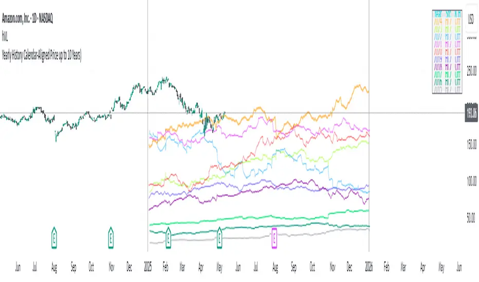
Sharpe & Sortino Ratio PROSharpe & Sortino Ratio PRO offers an advanced and more precise way to calculate and visualize the Sharpe and Sortino Ratios for financial assets on TradingView. Its main goal is to provide a scientifically accurate method for assessing the risk-adjusted performance of assets, both in the short and long term. Unlike TradingView’s built-in metrics, this script correctly handles periodic returns, uses optional logarithmic returns, properly annualizes both returns and volatility, and adjusts for the risk-free rate — all critical factors for truly meaningful Sharpe and Sortino calculations.
Users can customize the rolling analysis window (e.g., 252 periods for one year on daily data) and the long-term smoothing period (e.g., 1260 periods for five years). There’s also an option to select between linear and logarithmic returns and to manually input a risk-free rate if real-time data from FRED (the 3-Month T-Bill Rate via FRED:DGS3MO) is unavailable. Based on the chart’s timeframe (daily, weekly, or monthly), the script automatically adjusts the risk-free rate to a per-period basis.
The Sharpe Ratio is calculated by first determining the asset’s excess returns (returns after subtracting the risk-free return per period), then computing the average and standard deviation of those excess returns over the specified window, and finally annualizing these figures separately — in line with best scientific practices (Sharpe, 1994). The Sortino Ratio follows a similar approach but only considers negative returns, focusing specifically on downside risk (Sortino & Van der Meer, 1991).
To enhance readability, the script visualizes the ratios using a color gradient: strong negative values are shown in red, neutral values in yellow, and strong positive values in green. Additionally, the long-term averages for both Sharpe and Sortino are plotted with steady colors (teal and orange, respectively), making it easier to spot enduring performance trends.
Why calculating Sharpe and Sortino Ratios manually on TradingView is necessary?
While TradingView provides basic Sharpe and Sortino Ratios, they come with significant methodological flaws that can lead to misleading conclusions about an asset’s true risk-adjusted performance.
First, TradingView often computes volatility based on the standard deviation of price levels rather than returns (TradingView, 2023). This method is problematic because it causes the volatility measure to be directly dependent on the asset’s absolute price. For instance, a stock priced at $1,000 will naturally show larger absolute daily price moves than a $10 stock, even if their percentage changes are similar. This artificially inflates the measured standard deviation and, as a result, depresses the calculated Sharpe Ratio.
Second, TradingView frequently neglects to adjust for the risk-free rate. By treating all returns as risky returns, the computed Sharpe Ratio may significantly underestimate risk-adjusted performance, especially when interest rates are high (Sharpe, 1994).
Third, and perhaps most critically, TradingView doesn’t properly annualize the mean excess return and the standard deviation separately. In correct financial math, the mean excess return should be multiplied by the number of periods per year, while the standard deviation should be multiplied by the square root of the number of periods per year (Cont, 2001; Fabozzi et al., 2007). Incorrect annualization skews the Sharpe and Sortino Ratios and can lead to under- or overestimating investment risk.
These flaws lead to three major issues:
• Overstated volatility for high-priced assets.
• Incorrect scaling between returns and risk.
• Sharpe Ratios that are systematically biased downward, especially in high-price or high-interest environments.
How to properly calculate Sharpe and Sortino Ratios in Pine Script?
To get accurate results, the Sharpe and Sortino Ratios must be calculated using the correct methodology:
1. Use returns, not price levels, to calculate volatility. Ideally, use logarithmic returns for better mathematical properties like time additivity (Cont, 2001).
2. Adjust returns by subtracting the risk-free rate on a per-period basis to obtain true excess returns.
3. Annualize separately:
• Multiply the mean excess return by the number of periods per year (e.g., 252 for daily data).
• Multiply the standard deviation by the square root of the number of periods per year.
4. Finally, divide the annualized mean excess return by the annualized standard deviation to calculate the Sharpe Ratio.
The Sortino Ratio follows the same structure but uses downside deviations instead of standard deviations.
By following this scientifically sound method, you ensure that your Sharpe and Sortino Ratios truly reflect the asset’s real-world risk and return characteristics.
References
• Cont, R. (2001). Empirical properties of asset returns: stylized facts and statistical issues. Quantitative Finance, 1(2), pp. 223–236.
• Fabozzi, F.J., Gupta, F. and Markowitz, H.M. (2007). The Legacy of Modern Portfolio Theory. Journal of Investing, 16(3), pp. 7–22.
• Sharpe, W.F. (1994). The Sharpe Ratio. Journal of Portfolio Management, 21(1), pp. 49–58.
• Sortino, F.A. and Van der Meer, R. (1991). Downside Risk: Capturing What’s at Stake in Investment Situations. Journal of Portfolio Management, 17(4), pp. 27–31.
• TradingView (2023). Help Center - Understanding Sharpe and Sortino Ratios. Available at: www.tradingview.com (Accessed: 25 April 2025).
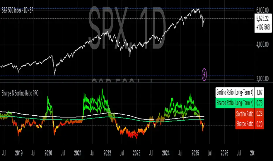
Date Display with Bar Counter and EMA===== ENGLISH DESCRIPTION =====
OVERVIEW:
This is a multi-function indicator that combines three useful tools in one script:
1. Date Display - Shows current date and symbol information in a customizable table
2. Bar Counter - Displays sequential bar numbers at specified intervals
3. EMA (Exponential Moving Average) - Plots an EMA line with customizable settings
FEATURES:
1. DATE DISPLAY:
- Shows date in full format (e.g., "Mon ∙ January 1, 2023") or short format (e.g., "Mon ∙ 01.01.23")
- Option to show/hide day of week
- Option to show/hide symbol and timeframe information
- Customizable table position (top/middle/bottom, left/center/right)
- Automatic color adjustment based on chart background
2. BAR COUNTER:
- Displays sequential bar numbers below price bars
- Customizable display frequency (every X bars)
- Special handling for Hong Kong futures (resets at market open)
- Different reset logic based on timeframe (daily, weekly, monthly)
- Customizable text size and color
3. EMA INDICATOR:
- Customizable period length (default: 20)
- Option to use different timeframe for calculation
- Option to wait for timeframe close for more stable signals
- Customizable line color
USAGE INSTRUCTIONS:
- After adding the indicator to your chart, customize settings in the "Format" panel
- The Date Display table will appear at your chosen position on the chart
- Bar numbers will appear below price bars at your specified frequency
- The EMA line will be plotted on the chart with your chosen settings
- Colors automatically adjust to light/dark chart themes
===== 中文说明 =====
概述:
这是一个多功能指标,将三个实用工具合并为一个脚本:
1. 日期显示 - 在可自定义的表格中显示当前日期和交易品种信息
2. K线计数器 - 按指定间隔显示K线序号
3. EMA指数移动平均线 - 绘制可自定义设置的EMA线
功能特点:
1. 日期显示:
- 支持完整格式(如"Mon ∙ January 1, 2023")或简短格式(如"Mon ∙ 01.01.23")
- 可选择显示/隐藏星期几
- 可选择显示/隐藏交易品种和时间周期信息
- 可自定义表格位置(顶部/中部/底部,左侧/中间/右侧)
- 根据图表背景自动调整颜色
2. K线计数器:
- 在价格K线下方显示序号
- 可自定义显示频率(每X根K线)
- 对香港期货有特殊处理(在开市时重置)
- 根据时间周期(日线、周线、月线)使用不同的重置逻辑
- 可自定义文字大小和颜色
3. EMA指标:
- 可自定义周期长度(默认:20)
- 可选择使用不同的时间周期进行计算
- 可选择等待时间周期结束以获得更稳定的信号
- 可自定义线条颜色
使用说明:
- 将指标添加到图表后,在"格式"面板中自定义设置
- 日期显示表格将出现在您选择的图表位置
- K线序号将按您指定的频率显示在价格K线下方
- EMA线将根据您选择的设置绘制在图表上
- 颜色会根据浅色/深色图表主题自动调整
*/

Gann & Fibonacci Analysis for MSTRYes! Below is a step-by-step guide to performing Gann Analysis on MSTR in TradingView for the last year.
Step 1: Set Up the Chart
Open TradingView and search for MSTR (MicroStrategy).
Select the 1-day (D) timeframe to analyze the past year.
Set your chart to logarithmic scale (⚙ Settings → Scale → Log).
Enable grid lines for alignment (⚙ Settings → Appearance → Grid Lines).
Step 2: Identify Key Highs and Lows (Last Year)
Find the 52-week high and 52-week low for MSTR.
As of now:
52-Week High: ~$999 (March 2024).
52-Week Low: ~$280 (October 2023).
Step 3: Plot Gann Angles
Using TradingView's Gann Fan Tool:
Select "Gann Fan" (Press / and type “Gann Fan” to find it).
Start at the 52-week low (~$280, October 2023) and drag upwards.
Adjust the angles to match key levels:
1x1 (45°) → Main trendline
2x1 (26.5°) → Strong uptrend
4x1 (15°) → Weak trendline
1x2 (63.75°) → Strong resistance
Repeat the process from the 52-week high (~$999, March 2024) downward to see bearish angles.
Step 4: Apply Fibonacci & Gann Retracement Levels
Using Fibonacci Retracement:
Select "Fibonacci Retracement" tool.
Draw from 52-week high ($999) to 52-week low ($280).
Enable key Fibonacci levels:
23.6% ($816)
38.2% ($678)
50% ($640)
61.8% ($550)
78.6% ($430)
Watch for price reactions near these levels.
Using Gann Retracement Levels:
Select "Gann Box" in TradingView.
Draw from 52-week high ($999) to low ($280).
Enable key Gann retracement levels:
12.5% ($912)
25% ($850)
37.5% ($768)
50% ($640)
62.5% ($550)
75% ($480)
87.5% ($350)
Identify confluences with Gann angles and Fibonacci levels.
Step 5: Identify Significant Dates & Time Cycles
Use "Date Range" Tool in TradingView.
Mark major turning points:
High → Low: ~180 days (Half-year cycle).
Low → High: ~90 days (Quarter cycle).
Use Square-Outs (Time = Price method):
Example: If MSTR hit $500, check 500 days from key events.
Mark key anniversaries of past highs/lows for possible reversals.
Step 6: Analyze and Trade Execution
✅ If MSTR is at a Gann angle + Fibonacci level + key date → Expect a reaction.
✅ Use RSI, MACD, and Volume for extra confirmation.
✅ Set Stop-Loss at nearest Gann support/resistance.

TASC 2025.02 Autocorrelation Indicator█ OVERVIEW
This script implements the Autocorrelation Indicator introduced by John Ehlers in the "Drunkard's Walk: Theory And Measurement By Autocorrelation" article from the February 2025 edition of TASC's Traders' Tips . The indicator calculates the autocorrelation of a price series across several lags to construct a periodogram , which traders can use to identify market cycles, trends, and potential reversal patterns.
█ CONCEPTS
Drunkard's walk
A drunkard's walk , formally known as a random walk , is a type of stochastic process that models the evolution of a system or variable through successive random steps.
In his article, John Ehlers relates this model to market data. He discusses two first- and second-order partial differential equations, modified for discrete (non-continuous) data, that can represent solutions to the discrete random walk problem: the diffusion equation and the wave equation. According to Ehlers, market data takes on a mixture of two "modes" described by these equations. He theorizes that when "diffusion mode" is dominant, trading success is almost a matter of luck, and when "wave mode" is dominant, indicators may have improved performance.
Pink spectrum
John Ehlers explains that many recent academic studies affirm that market data has a pink spectrum , meaning the power spectral density of the data is proportional to the wavelengths it contains, like pink noise . A random walk with a pink spectrum suggests that the states of the random variable are correlated and not independent. In other words, the random variable exhibits long-range dependence with respect to previous states.
Autocorrelation function (ACF)
Autocorrelation measures the correlation of a time series with a delayed copy, or lag , of itself. The autocorrelation function (ACF) is a method that evaluates autocorrelation across a range of lags , which can help to identify patterns, trends, and cycles in stochastic market data. Analysts often use ACF to detect and characterize long-range dependence in a time series.
The Autocorrelation Indicator evaluates the ACF of market prices over a fixed range of lags, expressing the results as a color-coded heatmap representing a dynamic periodogram. Ehlers suggests the information from the periodogram can help traders identify different market behaviors, including:
Cycles : Distinguishable as repeated patterns in the periodogram.
Reversals : Indicated by sharp vertical changes in the periodogram when the indicator uses a short data length .
Trends : Indicated by increasing correlation across lags, starting with the shortest, over time.
█ USAGE
This script calculates the Autocorrelation Indicator on an input "Source" series, smoothed by Ehlers' UltimateSmoother filter, and plots several color-coded lines to represent the periodogram's information. Each line corresponds to an analyzed lag, with the shortest lag's line at the bottom of the pane. Green hues in the line indicate a positive correlation for the lag, red hues indicate a negative correlation (anticorrelation), and orange or yellow hues mean the correlation is near zero.
Because Pine has a limit on the number of plots for a single indicator, this script divides the periodogram display into three distinct ranges that cover different lags. To see the full periodogram, add three instances of this script to the chart and set the "Lag range" input for each to a different value, as demonstrated in the chart above.
With a modest autocorrelation length, such as 20 on a "1D" chart, traders can identify seasonal patterns in the price series, which can help to pinpoint cycles and moderate trends. For instance, on the daily ES1! chart above, the indicator shows repetitive, similar patterns through fall 2023 and winter 2023-2024. The green "triangular" shape rising from the zero lag baseline over different time ranges corresponds to seasonal trends in the data.
To identify turning points in the price series, Ehlers recommends using a short autocorrelation length, such as 2. With this length, users can observe sharp, sudden shifts along the vertical axis, which suggest potential turning points from upward to downward or vice versa.

Star of David Drawing-AYNETExplanation of Code
Settings:
centerTime defines the center time for the star pattern, defaulting to January 1, 2023.
centerPrice is the center Y-axis level for positioning the star.
size controls the overall size of the star.
starColor and lineWidth allow customization of the color and thickness of the lines.
Utility Function:
toRadians converts degrees to radians, though it’s not directly used here, it might be useful for future adjustments to angles.
Star of David Drawing Function:
The drawStarOfDavid function calculates the position of each point on the star relative to the center coordinates (centerTime, centerY) and size.
The pattern has six key points that form two overlapping triangles, creating the Star of David pattern.
The time offsets (offset1 and offset2) determine the horizontal spread of the star, scaling according to size.
The line.new function is used to draw the star lines with the calculated coordinates, casting timestamps to int to comply with line.new requirements.
Star Rendering:
Finally, drawStarOfDavid is called to render the Star of David pattern on the chart based on the input parameters.
This code draws the Star of David on a chart at a specified time and price level, with customizable size, color, and line width. Adjust centerTime, centerPrice, and size as needed for different star placements on the chart.
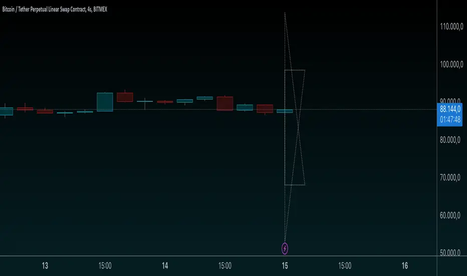
PE BandThe PE Band shows the highest and lowest P/E in the previous period with TTM EPS. If the current P/E is lower than the minimum P/E, it is considered cheap. In other words, higher than the maximum P/E is considered expensive.
PE Band consists of 2 lines.
- Firstly, the historical P/E value in "green" (if TTM EPS is positive) or "red" (if TTM EPS is negative) states will change according to the latest high or low price of TTM EPS, such as: :
After the second quarter of 2023 (end of June), how do prices from 1 July – 30 September reflect net profits? The program will get the highest and lowest prices during that time.
After the 3rd quarter of 2023 (end of September), how do prices from 1 Oct. - 31 Dec. reflect net profits? The program will get the highest and lowest prices during that time.
- Second, the blue line is the closing price divided by TTM EPS, which shows the current P/E.
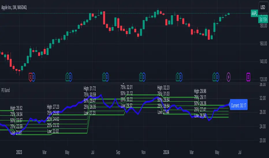
Backtest any Indicator v5Happy Trade,
here you get the opportunity to backtest any of your indicators like a strategy without converting them into a strategy. You can choose to go long or go short and detailed time filters. Further more you can set the take profit and stop loss, initial capital, quantity per trade and set the exchange fees. You get an overall result table and even a detailed, scroll-able table with all trades. In the Image 1 you see the provided info tables about all Trades and the Result Summary. Further more every trade is marked by a background color, Labels and Levels. An opening Label with the trade direction and trade number. A closing Label again with the trade number, the trades profit in % and the total amount of $ after all past trades. A green line for the take profit level and a red line for the stop loss.
Image 1
Example
For this description we choose the Stochastic RSI indicator from TradingView as it is. In Image 2 is shown the performance of it with decent settings.
Timeframe=45, BTCUSD, 2023-08-01 - 2023-10-20
Stoch RSI: k=30, d=40, RSI-length=140, stoch-length=140
Backtest any Indicator: input signal=Stoch RSI, goLong, take profit=9.1%, stop loss=2.5%, start capital=1000$, qty=5%, fee=0.1%, no Session Filter
Image 2
Usage
1) You need to know the name of the boolean (or integer) variable of your indicator which hold the buy condition. Lets say that this boolean variable is called BUY. If this BUY variable is not plotted on the chart you simply add the following code line at the end of your pine script.
For boolean (true/false) BUY variables use this:
plot(BUY ? 1:0,'Your buy condition hold in that variable BUY',display = display.data_window)
And in case your script's BUY variable is an integer or float then use instate the following code line:
plot(BUY ,'Your buy condition hold in that variable BUY',display = display.data_window)
2) Probably the name of this BUY variable in your indicator is not BUY. Simply replace in the code line above the BUY with the name of your script's trade condition variable.
3) Save your changed Indicator script.
4) Then add this 'Backtest any Indicator' script to the chart ...
5) and go to the settings of it. Choose under "Settings -> Buy Signal" your Indicator. So in the example above choose .
The form is usually: ' : BUY'. Then you see something like Image 2
6) Decide which trade direction the BUY signal should trigger. A go Long or a go Short by set the hook or not.
Now you have a backtest of your Indicator without converting it into a strategy. You may change the setting of your Indicator to the best results and setup the following strategy settings like Time- and Session Filter, Stop Loss, Take Profit etc. More of it below in the section Settings Menu.
Appereance
In the Image 2 you see on the right side the List of Trades . To scroll down you go into the settings again and decrease the scroll value. So you can see all trades that have happened before. In case there is an open trade you will find it at the last position of the list.
Every Long trade is green back grounded while Short trades are red.
Every trade begins with a label that show goLong or goShort and its number. And ends with another label again with its number, Profit in % and the resulting total amount of cash.
If activated you further see the Take Profit as a green line and the Stop Loss as a orange line. In the settings you can set their percentage above or below the entry price.
You also see the Result Summary below. Here you find the usual stats of a strategy of all closed trades. The profit after total amount of fees , amount of trades, Profit Factor and the total amount of fees .
Settings Menu
In the settings menu you will find the following high-lighted sections. Most of the settings have a question mark on their right side. Move over it with the cursor to read specific explanation.
Input Signal of your Indicator: Under Buy you set the trade signal of your Indicator. And under Target you set the value when a trade should happen. In the Example with the Stochastic RSI above we used 20. Below you can set the trade direction, let it be go short when hooked or go long when unhooked.
Trade Settings & List of Trades: Take Profit set the target price of any trade. Stop Loss set the price to step out when a trade goes the wrong direction. Check mark the List of Trades to see any single trade with their stats. In case that there are more trades as fits in the list you can scroll down the list by decrease the value Scroll .
Time Filter: You can set a Start Time or deactivate it by leave it unhooked. The same with End Time .
Session Filter: here you can choose to activate it on weekly base. Which days of the week should be trading and those without. And also on daily base from which time on and until trade are possible. Outside of all times and sessions there will be no new trades if activated.
Invest Settings: here you can choose the amount of cash to start with. The Quantity percentage define for every trade how much of the cash should be invested and the Fee percentage which have to be payed every trade. Open position and closing position.
Other Announcements
This Backtest script don't use the strategy functions of TradingView. It is programmed as an indicator. All trades get executed at candle closing. This script use the functionality "Indicator-on-Indicator" from TradingView.
Conclusion
So now it is your turn, take your promising indicators and connect it to that Backtest script. With it you get a fast impression of how successful your indicator will trade. You don't have to relay on coders who maybe add cheating code lines. Further more you can check with the Time Filter under which market condition you indicator perform the best or not so well. Also with the Session Filter you can sort out repeating good market conditions for your indicator. Even you can check with the GoShort XOR GoLong check mark the trade signals of you indicator in opposite trade direction with one click. And compare your indicators under the same conditions and get the results just after 2 clicks. Thanks to the in-build fee setting you get an impression how much a 0.1% fee cost you in total.
Cheers
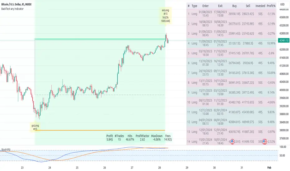
Bitcoin Google Trends OverlayThis indicator overlays Bitcoin Google trends data starting from 16/12/2018 until 10/12/2023. To have more recent data, you will need to update the data points manually.
If it is not showing properly, you need to plot the indicator to a new scale. Try also to use a logarithmic scale to better correlate the Bitcoin Google Trends data.
Interpretation:
Google Trends data and the Bitcoin price are very correlated. Google Trends data is a good indicator of market sentiment, but it usually lags.
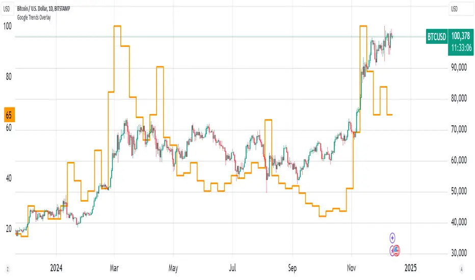
SuperTrend ToolkitThe SuperTrend Toolkit (Super Kit) introduces a versatile approach to trend analysis by extending the application of the SuperTrend indicator to a wide array of @TradingView's built-in or Community Scripts . This tool facilitates the integration of the SuperTrend algorithm with various indicators, including oscillators, moving averages, overlays, and channels.
Methodology:
The SuperTrend, at its core, calculates a trend-following indicator based on the Average-True-Range (ATR) and price action. It creates dynamic support and resistance levels, adjusting to changing market conditions, and aiding in trend identification.
pine_st(simple float factor = 3., simple int length = 10) =>
float atr = ta.atr(length)
float up = hl2 + factor * atr
up := up < nz(up ) or close > nz(up ) ? up : nz(up )
float lo = hl2 - factor * atr
lo := lo > nz(lo ) or close < nz(lo ) ? lo : nz(lo )
int dir = na
float st = na
if na(atr )
dir := 1
else if st == nz(up )
dir := close > up ? -1 : 1
else
dir := close < lo ? 1 : -1
st := dir == -1 ? lo : up
@TradingView's native SuperTrend lacks the flexibility to incorporate different price sources into its calculation.
Community scripts, addressed the limitation by implementing the option to input different price sources, for example, one of the most popular publications, @KivancOzbilgic's SuperTrend script.
In May 2023, @TradingView introduced an update allowing the passing of another indicator's plot as a source value via the input.source() function. However, the built-in ta.atr function still relied on the chart's price data, limiting the formerly mentioned scripts to the chart's price data alone.
Unique Approach -
This script addresses the aforementioned limitations by processing the data differently.
Firstly we create a User-Defined-Type (UDT) replicating a bar's open, high, low, close (OHLC) values.
type bar
float o = open
float h = high
float l = low
float c = close
We then use this type to store the external input data.
src = input.source(close, "External Source")
bar b = bar.new(
nz(src ) , open 𝘷𝘢𝘭𝘶𝘦
math.max(nz(src ), src), high 𝘷𝘢𝘭𝘶𝘦
math.min(nz(src ), src), low 𝘷𝘢𝘭𝘶𝘦
src ) close 𝘷𝘢𝘭𝘶𝘦
Finally, we pass the data into our custom built SuperTrend with ATR functions to derive the external source's version of the SuperTrend indicator.
supertrend st = b.st(mlt, len)
- Setup Guide -
Utility and Use Cases:
Universal Compatibility - Apply SuperTrend to any built-in indicator or script, expanding its use beyond traditional price data.
- A simple example on one of my own public scripts -
Trend Analysis - Gain additional trend insights into otherwise mainly mean reverting or volume indicators.
- Alerts Setup Guide -
The Super Kit empowers traders and analysts with a tool that adapts the robust SuperTrend algorithm to a myriad of indicators, allowing comprehensive trend analysis and strategy development.

TASC 2023.12 Growth and Value Switching System█ OVERVIEW
This script implements a rotation system for trading value and growth ETFs, as developed by Markos Katsanos and detailed in the article titled 'Growth Or Value?' in TASC's December 2023 edition of Traders' Tips . The purpose of this script is to demonstrate how short-term momentum can be employed to track market trends and provide clarity on when to switch between value and growth.
█ CONCEPTS
The central concept of the presented rotation strategy is based on the observation that the stock market undergoes cycles favoring either growth or value stocks. Consequently, the script introduces a momentum trading system that is designed to switch between value and growth equities based on prevailing market conditions. Specifically tailored for long-term index investors, the system focuses on trading Vanguard's value and growth ETFs ( VTV and VUG ) on a weekly timeframe.
To identify the ETF likely to outperform, the script uses a custom relative strength indicator applied to both VTV and VUG in comparison with an index ( SPY ). To minimize risk and drawdowns during bear markets, when both value and growth experience downtrends, the script employs the author's custom volume flow indicator (VFI) and blocks trades when its reading indicates money outflow . Positions are closed if the relative strength of the current open trade ETF falls below that of the other ETF for two consecutive weeks and is also below its moving average. Additionally, the script implements a stop-loss when the ETF is trading below its 40-week moving average, but only during bear markets.
The script plots the relative strengths of the value and growth equities along with the signals triggered by the aforementioned rules. Information about the current readings of the relative strength and volume flow indicators, along with the current open position, is displayed in a table.
█ CALCULATIONS
The script uses the request.security() function to gather price data for both equities and the reference index. Custom relative strength and volume flow indicators are calculated based on the formulas presented in the original article. By default, the script employs the same parameters for these indicators as proposed in the original article for VTV and VUG on a weekly timeframe.

TASC 2023.11 VAcc█ OVERVIEW
The November 2023 edition of TASC's Traders' Tips features an article titled "VAcc: A Momentum Indicator Based On Velocity And Acceleration" by Scott Cong. This script implements the author's momentum indicator based on simple physics concepts.
█ CONCEPTS
The indicator is named VAcc as it is derived from the average velocity (V) and acceleration (Acc) over a specified lookback period. Consequently, its readings reflect two valuable characteristics of price data: rate (indicating the speed at which the price is moving) and rate of change (indicating whether the price is speeding up or slowing down).
In the article, the author reports that for longer periods, VAcc behaves similarly to the MACD , albeit with a more responsive nature. For shorter periods, VAcc exhibits characteristics reminiscent of the stochastic oscillator , but it trends more prominently and is less prone to overbought/oversold saturation.
To incorporate VAcc into trading strategies, the author suggests considering the following two permutations for the velocity and acceleration data series:
Strong upward condition: Velocity is rising, and acceleration is rising above zero.
Strong downward condition: Velocity is falling, and acceleration is falling.
In the current implementation, the chart displays the average velocity as a line, while the average acceleration is presented as a histogram.
█ CALCULATIONS
The calculation of VAcc involves the following steps:
For the current closing price, C , and for each bar C (i) within a specified lookback period from the current bar, the script calculates velocities, V (i) = ( C - C (i))/i. These velocities are then subjected to an exponential moving average to obtain the smoothed average velocity.
Similarly, for each bar within the lookback period, accelerations are calculated as Acc (i) = ( V - V (i))/i and then averaged without smoothing.

TASC 2023.10 COT Commercials Indicator█ OVERVIEW
This script implements the COT Commercials Indicator introduced by Alfred François Tagher in an article featured in TASC's October 2023 edition of Traders' Tips . The indicator is designed for use in futures markets and represents a fast stochastic (%K) calculated based on the commercial open interest values of an asset derived from the weekly Commitments Of Traders (COT) report .
█ CONCEPTS
The COT report, issued by the Commodity Futures Trading Commission (CFTC) , presents a breakdown of reportable open interest positions held by various trader groups—commercial, noncommercial, and nonreportable (small traders). Open interest reflects the total number of derivative contracts entered by market participants but not yet settled. Consequently, it can serve as a measure of market activity and liquidity.
The indicator showcased here aims to analyze changes in the reported net values of open interest for commercial traders/hedgers (often referred to as 'smart money', as they deal directly in underlying commodities). The net values are positive when the commercial traders have more long positions than short ones and negative when they hold more short positions than long ones. Positive net values indicate that commercial traders hold more long positions than short ones, while negative values indicate the opposite. Thus, overbought and oversold conditions of the COT Commercials Indicator potentially suggest collective bullish and bearish sentiments, respectively.
█ CALCULATIONS
The calculations involve these steps:
1. Net open interest values are extracted from COT data using the LibraryCOT library provided by TradingView.
2. A fast stochastic indicator (%K) is then applied to normalize these net values.
The script also provides an option of calculating and plotting the indicator curve for noncommercial (speculators) open interest.
