PDF Smoothed Moving Average [BackQuant]PDF Smoothed Moving Average
Introducing BackQuant’s PDF Smoothed Moving Average (PDF-MA) — an innovative trading indicator that applies Probability Density Function (PDF) weighting to moving averages, creating a unique, trend-following tool that offers adaptive smoothing to price movements. This advanced indicator gives traders an edge by blending PDF-weighted values with conventional moving averages, helping to capture trend shifts with enhanced clarity.
Core Concept: Probability Density Function (PDF) Smoothing
The Probability Density Function (PDF) provides a mathematical approach to applying adaptive weighting to data points based on a specified variance and mean. In the PDF-MA indicator, the PDF function is used to weight price data, adding a layer of probabilistic smoothing that enhances the detection of trend strength while reducing noise.
The PDF weights are controlled by two key parameters:
Variance: Determines the spread of the weights, where higher values spread out the weighting effect, providing broader smoothing.
Mean : Centers the weights around a particular price value, influencing the trend’s directionality and sensitivity.
These PDF weights are applied to each price point over the chosen period, creating an adaptive and smooth moving average that more closely reflects the underlying price trend.
Blending PDF with Standard Moving Averages
To further improve the PDF-MA, this indicator combines the PDF-weighted average with a traditional moving average, selected by the user as either an Exponential Moving Average (EMA) or Simple Moving Average (SMA). This blended approach leverages the strengths of each method: the responsiveness of PDF smoothing and the robustness of conventional moving averages.
Smoothing Method: Traders can choose between EMA and SMA for the additional moving average layer. The EMA is more responsive to recent prices, while the SMA provides a consistent average across the selected period.
Smoothing Period: Controls the length of the lookback period, affecting how sensitive the average is to price changes.
The result is a PDF-MA that provides a reliable trend line, reflecting both the PDF weighting and traditional moving average values, ideal for use in trend-following and momentum-based strategies.
Trend Detection and Candle Coloring
The PDF-MA includes a built-in trend detection feature that dynamically colors candles based on the direction of the smoothed moving average:
Uptrend: When the PDF-MA value is increasing, the trend is considered bullish, and candles are colored green, indicating potential buying conditions.
Downtrend: When the PDF-MA value is decreasing, the trend is considered bearish, and candles are colored red, signaling potential selling or shorting conditions.
These color-coded candles provide a quick visual reference for the trend direction, helping traders make real-time decisions based on the current market trend.
Customization and Visualization Options
This indicator offers a range of customization options, allowing traders to tailor it to their specific preferences and trading environment:
Price Source : Choose the price data for calculation, with options like close, open, high, low, or HLC3.
Variance and Mean : Fine-tune the PDF weighting parameters to control the indicator’s sensitivity and responsiveness to price data.
Smoothing Method : Select either EMA or SMA to customize the conventional moving average layer used in conjunction with the PDF.
Smoothing Period : Set the lookback period for the moving average, with a longer period providing more stability and a shorter period offering greater sensitivity.
Candle Coloring : Enable or disable candle coloring based on trend direction, providing additional clarity in identifying bullish and bearish phases.
Trading Applications
The PDF Smoothed Moving Average can be applied across various trading strategies and timeframes:
Trend Following : By smoothing price data with PDF weighting, this indicator helps traders identify long-term trends while filtering out short-term noise.
Reversal Trading : The PDF-MA’s trend coloring feature can help pinpoint potential reversal points by showing shifts in the trend direction, allowing traders to enter or exit positions at optimal moments.
Swing Trading : The PDF-MA provides a clear trend line that swing traders can use to capture intermediate price moves, following the trend direction until it shifts.
Final Thoughts
The PDF Smoothed Moving Average is a highly adaptable indicator that combines probabilistic smoothing with traditional moving averages, providing a nuanced view of market trends. By integrating PDF-based weighting with the flexibility of EMA or SMA smoothing, this indicator offers traders an advanced tool for trend analysis that adapts to changing market conditions with reduced lag and increased accuracy.
Whether you’re trading trends, reversals, or swings, the PDF-MA offers valuable insights into the direction and strength of price movements, making it a versatile addition to any trading strategy.
在腳本中搜尋"长江电子+半导体行业研究框架培训+pdf"
ATR-Stepped PDF MA [Loxx]ATR-Stepped PDF MA is and ATR-stepped moving average that uses a probability density function moving average.
What is Probability Density Function?
Probability density function based MA is a sort of weighted moving average that uses probability density function to calculate the weights.
Included:
-Toggle on/off bar coloring
-Toggle on/off signals
-Alerts long/short
PDF MA For Loop [BackQuant]PDF MA For Loop
Introducing the PDF MA For Loop, an innovative trading indicator that combines Probability Density Function (PDF) smoothing with a dynamic for-loop scoring mechanism. This advanced tool provides traders with precise trend-following signals, helping to identify long and short opportunities with improved clarity and adaptability to market conditions.
If you would like to check out the stand alone PDF Moving Average:
Core Concept: Probability Density Function (PDF) Smoothing
The PDF smoothing method is a unique approach that applies adaptive weights to price data based on a Probability Density Function. This ensures that recent data points receive appropriate emphasis while maintaining a smooth transition across the data set. The result is a moving average that is not only smoother but also more responsive to market changes.
Key parameters in PDF smoothing:
Variance : Controls the spread of the PDF, where a higher value results in broader smoothing and a lower value makes the moving average more sensitive.
Mean : Centers the PDF around a specific value, influencing the weighting and responsiveness of the smoothing process.
By combining PDF smoothing with traditional moving averages (EMA or SMA), the indicator creates a hybrid signal that balances responsiveness and reliability.
For-Loop Scoring Mechanism
At the heart of this indicator is the for-loop scoring mechanism, which evaluates the smoothed PDF moving average over a defined range of historical data points. This process assigns a score to the current market condition based on whether the PDF moving average is greater than or less than previous values.
Long Signal: A long signal is generated when the score exceeds the Long Threshold (default set at 40), indicating upward momentum.
Short Signal: A short signal is triggered when the score crosses below the Short Threshold (default set at -10), suggesting potential downward momentum.
This dynamic scoring system ensures that the indicator remains adaptive, capturing trends and shifts in market sentiment effectively.
Customization Options
The PDF MA For Loop includes a variety of customizable settings to fit different trading styles and strategies:
Calculation Settings
Price Source : Select the input price for the calculation (default is the close price).
Smoothing Method : Choose between EMA or SMA for the additional smoothing layer, providing flexibility to adapt to market conditions.
Smoothing Period : Adjust the lookback period for the smoothing function, with shorter periods providing more sensitivity and longer periods offering greater stability.
Variance & Mean : Fine-tune the PDF function parameters to control the weighting of the smoothing process.
Signal Settings
Thresholds : Customize the upper and lower thresholds to define the sensitivity of the long and short signals.
For Loop Range : Set the range of historical data points analyzed by the for-loop, influencing the depth of the scoring mechanism.
UI Settings
Signal Line Width: Adjust the thickness of the plotted signal line for better visibility.
Candle Coloring: Enable or disable the coloring of candlesticks based on trend direction (green for long, red for short, gray for neutral).
Background Coloring: Add background shading to highlight long and short signals for an enhanced visual experience.
Alerts and Automation
The indicator includes built-in alert conditions to notify traders of important market events:
Long Signal Alert: Notifies when the score exceeds the upper threshold, indicating a bullish trend.
Short Signal Alert: Notifies when the score crosses below the lower threshold, signaling a bearish trend.
These alerts can be configured for real-time notifications, allowing traders to respond quickly to market changes without constant chart monitoring.
Trading Applications
The PDF MA For Loop is versatile and can be applied across various trading strategies and market conditions:
Trend Following: The PDF smoothing method combined with for-loop scoring makes this indicator particularly effective for identifying and following trends.
Reversal Trading: By observing the thresholds and score, traders can anticipate potential reversals when the trend shifts from long to short (or vice versa).
Risk Management: The dynamic thresholds and scoring provide clear signals, allowing traders to enter and exit trades with greater confidence and precision.
Final Thoughts
The PDF MA For Loopis merges advanced mathematical concepts with practical trading tools. By leveraging Probability Density Function smoothing and a dynamic for-loop scoring system, it provides traders with clear, actionable signals while adapting to market conditions.
Whether you’re looking for an edge in trend-following strategies or seeking precision in identifying reversals, this indicator offers the flexibility and power to enhance your trading decisions
As always, backtesting and integrating the PDF MA For Loop into a comprehensive trading strategy is recommended for optimal performance, as no single indicator should be used in isolation.
Thus following all of the key points here are some sample backtests on the 1D Chart
Disclaimer: Backtests are based off past results, and are not indicative of the future.
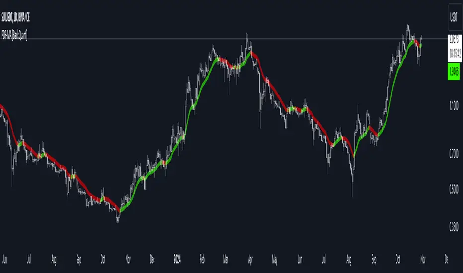
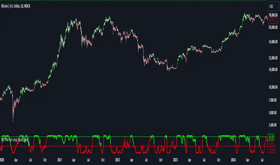
INDEX:BTCUSD
INDEX:ETHUSD
BINANCE:SOLUSD
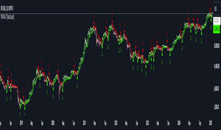
PDF-MA Supertrend [BackQuant]PDF-MA Supertrend
The PDF-MA Supertrend combines the innovative Probability Density Function (PDF) smoothing with the widely popular Supertrend methodology, creating a robust tool for identifying trends and generating actionable trading signals. This indicator is designed to provide precise entries and exits by dynamically adapting to market volatility while visualizing long and short opportunities directly on the chart.
Core Feature: PDF Smoothing
At the foundation of this indicator is the PDF smoothing technique, which applies a Probability Density Function to calculate a smoothed moving average. This method allows the indicator to assign adaptive weights to data points, making it responsive to market changes without overreacting to short-term volatility.
Key parameters include:
Variance: Controls the spread of the PDF weighting. A smaller variance results in sharper responses, while a larger variance smooths out the curve.
Mean: Shifts the PDF’s center, allowing traders to tweak how weights are distributed around the data points.
Smoothing Method: Offers the choice between EMA (Exponential Moving Average) and SMA (Simple Moving Average) for blending the PDF-smoothed data with traditional moving average methods.
By combining these parameters, the PDF smoothing creates a moving average that effectively captures underlying trends.
Supertrend: Adaptive Trend and Volatility Tracking
The Supertrend is a well-known volatility-based indicator that dynamically adjusts to market conditions using the ATR (Average True Range). In this script, the PDF-smoothed moving average acts as the price input, making the Supertrend calculation more adaptive and precise.
Key Supertrend Features:
ATR Period: Determines the lookback period for calculating market volatility.
Factor: Multiplies the ATR to set the distance between the Supertrend and the price. A higher factor creates wider bands, filtering out smaller price movements, while a lower factor captures tighter trends.
Dynamic Direction: The Supertrend flips its direction based on price interactions with the calculated upper and lower bands:
Uptrend : When the price is above the Supertrend, the direction turns bullish.
Downtrend : When the price is below the Supertrend, the direction turns bearish.
This combination of PDF smoothing and Supertrend calculation ensures that trends are detected with greater accuracy, while volatility filters out market noise.
Long and Short Signal Generation
The PDF-MA Supertrend generates actionable trading signals by detecting transitions in the trend direction:
Long Signal (𝕃): Triggered when the trend transitions from bearish to bullish. This is visually represented with a green triangle below the price bars.
Short Signal (𝕊): Triggered when the trend transitions from bullish to bearish. This is marked with a red triangle above the price bars.
These signals provide traders with clear entry and exit points, ensuring they can capitalize on emerging trends while avoiding false signals.
Customizable Visualization Options
The indicator offers a range of visualization settings to help traders interpret the data with ease:
Show Supertrend: Option to toggle the visibility of the Supertrend line.
Candle Coloring: Automatically colors candlesticks based on the trend direction:
Green for long trends.
Red for short trends.
Long and Short Signals (𝕃 + 𝕊): Displays long (𝕃) and short (𝕊) signals directly on the chart for quick identification of trade opportunities.
Line Color Customization: Allows users to customize the colors for long and short trends.
Alert Conditions
To ensure traders never miss an opportunity, the PDF-MA Supertrend includes built-in alerts for trend changes:
Long Signal Alert: Notifies when a bullish trend is identified.
Short Signal Alert: Notifies when a bearish trend is identified.
These alerts can be configured for real-time notifications via SMS, email, or push notifications, making it easier to stay updated on market movements.
Suggested Parameter Adjustments
The indicator’s effectiveness can be fine-tuned using the following guidelines:
Variance:
For low-volatility assets (e.g., indices): Use a smaller variance (1.0–1.5) for smoother trends.
For high-volatility assets (e.g., cryptocurrencies): Use a larger variance (1.5–2.0) to better capture rapid price changes.
ATR Factor:
A higher factor (e.g., 2.0) is better suited for long-term trend-following strategies.
A lower factor (e.g., 1.5) captures shorter-term trends.
Smoothing Period:
Shorter periods provide more reactive signals but may increase noise.
Longer periods offer stability and better alignment with significant trends.
Experimentation is encouraged to find the optimal settings for specific assets and trading strategies.
Trading Applications
The PDF-MA Supertrend is a versatile indicator suited to a variety of trading approaches:
Trend Following : Use the Supertrend line and signals to follow market trends and ride sustained price movements.
Reversal Trading : Spot potential trend reversals as the Supertrend flips direction.
Volatility Analysis : Adjust the ATR factor to filter out minor price fluctuations or capture sharp movements.
Final Thoughts
The PDF-MA Supertrend combines the precision of Probability Density Function smoothing with the adaptability of the Supertrend methodology, offering traders a powerful tool for identifying trends and volatility. With its customizable parameters, actionable signals, and built-in alerts, this indicator is an excellent choice for traders seeking a robust and reliable system for trend detection and entry/exit timing.
As always, backtesting and incorporating this indicator into a broader strategy are recommended for optimal results.
LibVPrfLibrary "LibVPrf"
This library provides an object-oriented framework for volume
profile analysis in Pine Script®. It is built around the `VProf`
User-Defined Type (UDT), which encapsulates all data, settings,
and statistical metrics for a single profile, enabling stateful
analysis with on-demand calculations.
Key Features:
1. **Object-Oriented Design (UDT):** The library is built around
the `VProf` UDT. This object encapsulates all profile data
and provides methods for its full lifecycle management,
including creation, cloning, clearing, and merging of profiles.
2. **Volume Allocation (`AllotMode`):** Offers two methods for
allocating a bar's volume:
- **Classic:** Assigns the entire bar's volume to the close
price bucket.
- **PDF:** Distributes volume across the bar's range using a
statistical price distribution model from the `LibBrSt` library.
3. **Buy/Sell Volume Splitting (`SplitMode`):** Provides methods
for classifying volume into buying and selling pressure:
- **Classic:** Classifies volume based on the bar's color (Close vs. Open).
- **Dynamic:** A specific model that analyzes candle structure
(body vs. wicks) and a short-term trend factor to
estimate the buy/sell share at each price level.
4. **Statistical Analysis (On-Demand):** Offers a suite of
statistical metrics calculated using a "Lazy Evaluation"
pattern (computed only when requested via `get...` methods):
- **Central Tendency:** Point of Control (POC), VWAP, and Median.
- **Dispersion:** Value Area (VA) and Population Standard Deviation.
- **Shape:** Skewness and Excess Kurtosis.
- **Delta:** Cumulative Volume Delta, including its
historical high/low watermarks.
5. **Structural Analysis:** Includes a parameter-free method
(`getSegments`) to decompose a profile into its fundamental
unimodal segments, allowing for modality detection (e.g.,
identifying bimodal profiles).
6. **Dynamic Profile Management:**
- **Auto-Fitting:** Profiles set to `dynamic = true` will
automatically expand their price range to fit new data.
- **Manipulation:** The resolution, price range, and Value Area
of a dynamic profile can be changed at any time. This
triggers a resampling process that uses a **linear
interpolation model** to re-bucket existing volume.
- **Assumption:** Non-dynamic profiles are fixed and will throw
a `runtime.error` if `addBar` is called with data
outside their initial range.
7. **Bucket-Level Access:** Provides getter methods for direct
iteration and analysis of the raw buy/sell volume and price
boundaries of each individual price bucket.
---
**DISCLAIMER**
This library is provided "AS IS" and for informational and
educational purposes only. It does not constitute financial,
investment, or trading advice.
The author assumes no liability for any errors, inaccuracies,
or omissions in the code. Using this library to build
trading indicators or strategies is entirely at your own risk.
As a developer using this library, you are solely responsible
for the rigorous testing, validation, and performance of any
scripts you create based on these functions. The author shall
not be held liable for any financial losses incurred directly
or indirectly from the use of this library or any scripts
derived from it.
create(buckets, rangeUp, rangeLo, dynamic, valueArea, allot, estimator, cdfSteps, split, trendLen)
Construct a new `VProf` object with fixed bucket count & range.
Parameters:
buckets (int) : series int number of price buckets ≥ 1
rangeUp (float) : series float upper price bound (absolute)
rangeLo (float) : series float lower price bound (absolute)
dynamic (bool) : series bool Flag for dynamic adaption of profile ranges
valueArea (int) : series int Percentage of total volume to include in the Value Area (1..100)
allot (series AllotMode) : series AllotMode Allocation mode `classic` or `pdf` (default `classic`)
estimator (series PriceEst enum from AustrianTradingMachine/LibBrSt/1) : series LibBrSt.PriceEst PDF model when `model == PDF`. (deflault = 'uniform')
cdfSteps (int) : series int even #sub-intervals for Simpson rule (default 20)
split (series SplitMode) : series SplitMode Buy/Sell determination (default `classic`)
trendLen (int) : series int Look‑back bars for trend factor (default 3)
Returns: VProf freshly initialised profile
method clone(self)
Create a deep copy of the volume profile.
Namespace types: VProf
Parameters:
self (VProf) : VProf Profile object to copy
Returns: VProf A new, independent copy of the profile
method clear(self)
Reset all bucket tallies while keeping configuration intact.
Namespace types: VProf
Parameters:
self (VProf) : VProf profile object
Returns: VProf cleared profile (chaining)
method merge(self, srcABuy, srcASell, srcRangeUp, srcRangeLo, srcCvd, srcCvdHi, srcCvdLo)
Merges volume data from a source profile into the current profile.
If resizing is needed, it performs a high-fidelity re-bucketing of existing
volume using a linear interpolation model inferred from neighboring buckets,
preventing aliasing artifacts and ensuring accurate volume preservation.
Namespace types: VProf
Parameters:
self (VProf) : VProf The target profile object to merge into.
srcABuy (array) : array The source profile's buy volume bucket array.
srcASell (array) : array The source profile's sell volume bucket array.
srcRangeUp (float) : series float The upper price bound of the source profile.
srcRangeLo (float) : series float The lower price bound of the source profile.
srcCvd (float) : series float The final Cumulative Volume Delta (CVD) value of the source profile.
srcCvdHi (float) : series float The historical high-water mark of the CVD from the source profile.
srcCvdLo (float) : series float The historical low-water mark of the CVD from the source profile.
Returns: VProf `self` (chaining), now containing the merged data.
method addBar(self, offset)
Add current bar’s volume to the profile (call once per realtime bar).
classic mode: allocates all volume to the close bucket and classifies
by `close >= open`. PDF mode: distributes volume across buckets by the
estimator’s CDF mass. For `split = dynamic`, the buy/sell share per
price is computed via context-driven piecewise s(u).
Namespace types: VProf
Parameters:
self (VProf) : VProf Profile object
offset (int) : series int To offset the calculated bar
Returns: VProf `self` (method chaining)
method setBuckets(self, buckets)
Sets the number of buckets for the volume profile.
Behavior depends on the `isDynamic` flag.
- If `dynamic = true`: Works on filled profiles by re-bucketing to a new resolution.
- If `dynamic = false`: Only works on empty profiles to prevent accidental changes.
Namespace types: VProf
Parameters:
self (VProf) : VProf Profile object
buckets (int) : series int The new number of buckets
Returns: VProf `self` (chaining)
method setRanges(self, rangeUp, rangeLo)
Sets the price range for the volume profile.
Behavior depends on the `dynamic` flag.
- If `dynamic = true`: Works on filled profiles by re-bucketing existing volume.
- If `dynamic = false`: Only works on empty profiles to prevent accidental changes.
Namespace types: VProf
Parameters:
self (VProf) : VProf Profile object
rangeUp (float) : series float The new upper price bound
rangeLo (float) : series float The new lower price bound
Returns: VProf `self` (chaining)
method setValueArea(self, valueArea)
Set the percentage of volume for the Value Area. If the value
changes, the profile is finalized again.
Namespace types: VProf
Parameters:
self (VProf) : VProf Profile object
valueArea (int) : series int The new Value Area percentage (0..100)
Returns: VProf `self` (chaining)
method getBktBuyVol(self, idx)
Get Buy volume of a bucket.
Namespace types: VProf
Parameters:
self (VProf) : VProf Profile object
idx (int) : series int Bucket index
Returns: series float Buy volume ≥ 0
method getBktSellVol(self, idx)
Get Sell volume of a bucket.
Namespace types: VProf
Parameters:
self (VProf) : VProf Profile object
idx (int) : series int Bucket index
Returns: series float Sell volume ≥ 0
method getBktBnds(self, idx)
Get Bounds of a bucket.
Namespace types: VProf
Parameters:
self (VProf) : VProf Profile object
idx (int) : series int Bucket index
Returns:
up series float The upper price bound of the bucket.
lo series float The lower price bound of the bucket.
method getPoc(self)
Get POC information.
Namespace types: VProf
Parameters:
self (VProf) : VProf Profile object
Returns:
pocIndex series int The index of the Point of Control (POC) bucket.
pocPrice. series float The mid-price of the Point of Control (POC) bucket.
method getVA(self)
Get Value Area (VA) information.
Namespace types: VProf
Parameters:
self (VProf) : VProf Profile object
Returns:
vaUpIndex series int The index of the upper bound bucket of the Value Area.
vaUpPrice series float The upper price bound of the Value Area.
vaLoIndex series int The index of the lower bound bucket of the Value Area.
vaLoPrice series float The lower price bound of the Value Area.
method getMedian(self)
Get the profile's median price and its bucket index. Calculates the value on-demand if stale.
Namespace types: VProf
Parameters:
self (VProf) : VProf Profile object.
Returns:
medianIndex series int The index of the bucket containing the Median.
medianPrice series float The Median price of the profile.
method getVwap(self)
Get the profile's VWAP and its bucket index. Calculates the value on-demand if stale.
Namespace types: VProf
Parameters:
self (VProf) : VProf Profile object.
Returns:
vwapIndex series int The index of the bucket containing the VWAP.
vwapPrice series float The Volume Weighted Average Price of the profile.
method getStdDev(self)
Get the profile's volume-weighted standard deviation. Calculates the value on-demand if stale.
Namespace types: VProf
Parameters:
self (VProf) : VProf Profile object.
Returns: series float The Standard deviation of the profile.
method getSkewness(self)
Get the profile's skewness. Calculates the value on-demand if stale.
Namespace types: VProf
Parameters:
self (VProf) : VProf Profile object.
Returns: series float The Skewness of the profile.
method getKurtosis(self)
Get the profile's excess kurtosis. Calculates the value on-demand if stale.
Namespace types: VProf
Parameters:
self (VProf) : VProf Profile object.
Returns: series float The Kurtosis of the profile.
method getSegments(self)
Get the profile's fundamental unimodal segments. Calculates on-demand if stale.
Uses a parameter-free, pivot-based recursive algorithm.
Namespace types: VProf
Parameters:
self (VProf) : VProf The profile object.
Returns: matrix A 2-column matrix where each row is an pair.
method getCvd(self)
Cumulative Volume Delta (CVD) like metric over all buckets.
Namespace types: VProf
Parameters:
self (VProf) : VProf Profile object.
Returns:
cvd series float The final Cumulative Volume Delta (Total Buy Vol - Total Sell Vol).
cvdHi series float The running high-water mark of the CVD as volume was added.
cvdLo series float The running low-water mark of the CVD as volume was added.
VProf
VProf Bucketed Buy/Sell volume profile plus meta information.
Fields:
buckets (series int) : int Number of price buckets (granularity ≥1)
rangeUp (series float) : float Upper price range (absolute)
rangeLo (series float) : float Lower price range (absolute)
dynamic (series bool) : bool Flag for dynamic adaption of profile ranges
valueArea (series int) : int Percentage of total volume to include in the Value Area (1..100)
allot (series AllotMode) : AllotMode Allocation mode `classic` or `pdf`
estimator (series PriceEst enum from AustrianTradingMachine/LibBrSt/1) : LibBrSt.PriceEst Price density model when `model == PDF`
cdfSteps (series int) : int Simpson integration resolution (even ≥2)
split (series SplitMode) : SplitMode Buy/Sell split strategy per bar
trendLen (series int) : int Look‑back length for trend factor (≥1)
maxBkt (series int) : int User-defined number of buckets (unclamped)
aBuy (array) : array Buy volume per bucket
aSell (array) : array Sell volume per bucket
cvd (series float) : float Final Cumulative Volume Delta (Total Buy Vol - Total Sell Vol).
cvdHi (series float) : float Running high-water mark of the CVD as volume was added.
cvdLo (series float) : float Running low-water mark of the CVD as volume was added.
poc (series int) : int Index of max‑volume bucket (POC). Is `na` until calculated.
vaUp (series int) : int Index of upper Value‑Area bound. Is `na` until calculated.
vaLo (series int) : int Index of lower value‑Area bound. Is `na` until calculated.
median (series float) : float Median price of the volume distribution. Is `na` until calculated.
vwap (series float) : float Profile VWAP (Volume Weighted Average Price). Is `na` until calculated.
stdDev (series float) : float Standard Deviation of volume around the VWAP. Is `na` until calculated.
skewness (series float) : float Skewness of the volume distribution. Is `na` until calculated.
kurtosis (series float) : float Excess Kurtosis of the volume distribution. Is `na` until calculated.
segments (matrix) : matrix A 2-column matrix where each row is an pair. Is `na` until calculated.

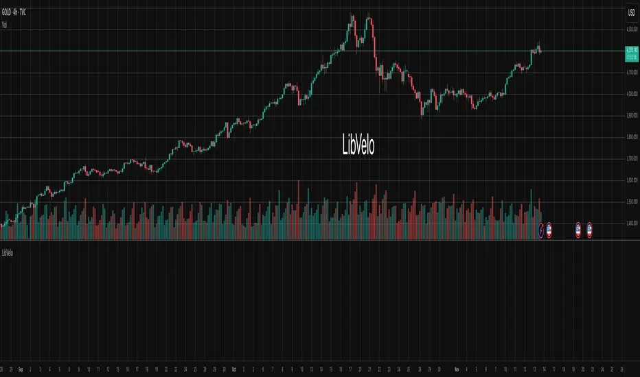
LibVeloLibrary "LibVelo"
This library provides a sophisticated framework for **Velocity
Profile (Flow Rate)** analysis. It measures the physical
speed of trading at specific price levels by relating volume
to the time spent at those levels.
## Core Concept: Market Velocity
Unlike Volume Profiles, which only answer "how much" traded,
Velocity Profiles answer "how fast" it traded.
It is calculated as:
`Velocity = Volume / Duration`
This metric (contracts per second) reveals hidden market
dynamics invisible to pure Volume or TPO profiles:
1. **High Velocity (Fast Flow):**
* **Aggression:** Initiative buyers/sellers hitting market
orders rapidly.
* **Liquidity Vacuum:** Price slips through a level because
order book depth is thin (low resistance).
2. **Low Velocity (Slow Flow):**
* **Absorption:** High volume but very slow price movement.
Indicates massive passive limit orders ("Icebergs").
* **Apathy:** Little volume over a long time. Lack of
interest from major participants.
## Architecture: Triple-Engine Composition
To ensure maximum performance while offering full statistical
depth for all metrics, this library utilises **object
composition** with a lazy evaluation strategy:
#### Engine A: The Master (`vpVol`)
* **Role:** Standard Volume Profile.
* **Purpose:** Maintains the "ground truth" of volume distribution,
price buckets, and ranges.
#### Engine B: The Time Container (`vpTime`)
* **Role:** specialized container for time duration (in ms).
* **Hack:** It repurposes standard volume arrays (specifically
`aBuy`) to accumulate time duration for each bucket.
#### Engine C: The Calculator (`vpVelo`)
* **Role:** Temporary scratchpad for derived metrics.
* **Purpose:** When complex statistics (like Value Area or Skewness)
are requested for **Velocity**, this engine is assembled
on-demand to leverage the full statistical power of `LibVPrf`
without rewriting complex algorithms.
---
**DISCLAIMER**
This library is provided "AS IS" and for informational and
educational purposes only. It does not constitute financial,
investment, or trading advice.
The author assumes no liability for any errors, inaccuracies,
or omissions in the code. Using this library to build
trading indicators or strategies is entirely at your own risk.
As a developer using this library, you are solely responsible
for the rigorous testing, validation, and performance of any
scripts you create based on these functions. The author shall
not be held liable for any financial losses incurred directly
or indirectly from the use of this library or any scripts
derived from it.
create(buckets, rangeUp, rangeLo, dynamic, valueArea, allot, estimator, cdfSteps, split, trendLen)
Construct a new `Velo` controller, initializing its engines.
Parameters:
buckets (int) : series int Number of price buckets ≥ 1.
rangeUp (float) : series float Upper price bound (absolute).
rangeLo (float) : series float Lower price bound (absolute).
dynamic (bool) : series bool Flag for dynamic adaption of profile ranges.
valueArea (int) : series int Percentage for Value Area (1..100).
allot (series AllotMode) : series AllotMode Allocation mode `Classic` or `PDF` (default `PDF`).
estimator (series PriceEst enum from AustrianTradingMachine/LibBrSt/1) : series PriceEst PDF model for distribution attribution (default `Uniform`).
cdfSteps (int) : series int Resolution for PDF integration (default 20).
split (series SplitMode) : series SplitMode Buy/Sell split for the master volume engine (default `Classic`).
trendLen (int) : series int Look‑back for trend factor in dynamic split (default 3).
Returns: Velo Freshly initialised velocity profile.
method clone(self)
Create a deep copy of the composite profile.
Namespace types: Velo
Parameters:
self (Velo) : Velo Profile object to copy.
Returns: Velo A completely independent clone.
method clear(self)
Reset all engines and accumulators.
Namespace types: Velo
Parameters:
self (Velo) : Velo Profile object to clear.
Returns: Velo Cleared profile (chaining).
method merge(self, srcVolBuy, srcVolSell, srcTime, srcRangeUp, srcRangeLo, srcVolCvd, srcVolCvdHi, srcVolCvdLo)
Merges external data (Volume and Time) into the current profile.
Automatically handles resizing and re-bucketing if ranges differ.
Namespace types: Velo
Parameters:
self (Velo) : Velo The profile object.
srcVolBuy (array) : array Source Buy Volume bucket array.
srcVolSell (array) : array Source Sell Volume bucket array.
srcTime (array) : array Source Time bucket array (ms).
srcRangeUp (float) : series float Upper price bound of the source data.
srcRangeLo (float) : series float Lower price bound of the source data.
srcVolCvd (float) : series float Source Volume CVD final value.
srcVolCvdHi (float) : series float Source Volume CVD High watermark.
srcVolCvdLo (float) : series float Source Volume CVD Low watermark.
Returns: Velo `self` (chaining).
method addBar(self, offset)
Main data ingestion. Distributes Volume and Time to buckets.
Namespace types: Velo
Parameters:
self (Velo) : Velo The profile object.
offset (int) : series int Offset of the bar to add (default 0).
Returns: Velo `self` (chaining).
method setBuckets(self, buckets)
Sets the number of buckets for the profile.
Namespace types: Velo
Parameters:
self (Velo) : Velo The profile object.
buckets (int) : series int New number of buckets.
Returns: Velo `self` (chaining).
method setRanges(self, rangeUp, rangeLo)
Sets the price range for the profile.
Namespace types: Velo
Parameters:
self (Velo) : Velo The profile object.
rangeUp (float) : series float New upper price bound.
rangeLo (float) : series float New lower price bound.
Returns: Velo `self` (chaining).
method setValueArea(self, va)
Set the percentage of volume/time for the Value Area.
Namespace types: Velo
Parameters:
self (Velo) : Velo The profile object.
va (int) : series int New Value Area percentage (0..100).
Returns: Velo `self` (chaining).
method getBuckets(self)
Returns the current number of buckets in the profile.
Namespace types: Velo
Parameters:
self (Velo) : Velo The profile object.
Returns: series int The number of buckets.
method getRanges(self)
Returns the current price range of the profile.
Namespace types: Velo
Parameters:
self (Velo) : Velo The profile object.
Returns:
rangeUp series float The upper price bound of the profile.
rangeLo series float The lower price bound of the profile.
method getArrayBuyVol(self)
Returns the internal raw data array for **Buy Volume** directly.
Namespace types: Velo
Parameters:
self (Velo) : Velo The profile object.
Returns: array The internal array for buy volume.
method getArraySellVol(self)
Returns the internal raw data array for **Sell Volume** directly.
Namespace types: Velo
Parameters:
self (Velo) : Velo The profile object.
Returns: array The internal array for sell volume.
method getArrayTime(self)
Returns the internal raw data array for **Time** (in ms) directly.
Namespace types: Velo
Parameters:
self (Velo) : Velo The profile object.
Returns: array The internal array for time duration.
method getArrayBuyVelo(self)
Returns the internal raw data array for **Buy Velocity** directly.
Automatically executes _assemble() if data is dirty.
Namespace types: Velo
Parameters:
self (Velo) : Velo The profile object.
Returns: array The internal array for buy velocity.
method getArraySellVelo(self)
Returns the internal raw data array for **Sell Velocity** directly.
Automatically executes _assemble() if data is dirty.
Namespace types: Velo
Parameters:
self (Velo) : Velo The profile object.
Returns: array The internal array for sell velocity.
method getBucketBuyVol(self, idx)
Returns the **Buy Volume** of a specific bucket.
Namespace types: Velo
Parameters:
self (Velo) : Velo The profile object.
idx (int) : series int The index of the bucket.
Returns: series float The buy volume.
method getBucketSellVol(self, idx)
Returns the **Sell Volume** of a specific bucket.
Namespace types: Velo
Parameters:
self (Velo) : Velo The profile object.
idx (int) : series int The index of the bucket.
Returns: series float The sell volume.
method getBucketTime(self, idx)
Returns the raw accumulated time (in ms) spent in a specific bucket.
Namespace types: Velo
Parameters:
self (Velo) : Velo The profile object.
idx (int) : series int The index of the bucket.
Returns: series float The time in milliseconds.
method getBucketBuyVelo(self, idx)
Returns the **Buy Velocity** (Aggressive Buy Flow) of a bucket.
Namespace types: Velo
Parameters:
self (Velo) : Velo The profile object.
idx (int) : series int The index of the bucket.
Returns: series float The buy velocity in .
method getBucketSellVelo(self, idx)
Returns the **Sell Velocity** (Aggressive Sell Flow) of a bucket.
Namespace types: Velo
Parameters:
self (Velo) : Velo The profile object.
idx (int) : series int The index of the bucket.
Returns: series float The sell velocity in .
method getBktBnds(self, idx)
Returns the price boundaries of a specific bucket.
Namespace types: Velo
Parameters:
self (Velo) : Velo The profile object.
idx (int) : series int The index of the bucket.
Returns:
up series float The upper price bound of the bucket.
lo series float The lower price bound of the bucket.
method getPoc(self, target)
Returns Point of Control (POC) information for the specified target metric.
Calculates on-demand if the target is 'Velocity' and data changed.
Namespace types: Velo
Parameters:
self (Velo) : Velo The profile object.
target (series Metric) : Metric The data aspect to analyse (Volume, Time, Velocity).
Returns:
pocIdx series int The index of the POC bucket.
pocPrice series float The mid-price of the POC bucket.
method getVA(self, target)
Returns Value Area (VA) information for the specified target metric.
Calculates on-demand if the target is 'Velocity' and data changed.
Namespace types: Velo
Parameters:
self (Velo) : Velo The profile object.
target (series Metric) : Metric The data aspect to analyse (Volume, Time, Velocity).
Returns:
vaUpIdx series int The index of the upper VA bucket.
vaUpPrice series float The upper price bound of the VA.
vaLoIdx series int The index of the lower VA bucket.
vaLoPrice series float The lower price bound of the VA.
method getMedian(self, target)
Returns the Median price for the specified target metric distribution.
Calculates on-demand if the target is 'Velocity' and data changed.
Namespace types: Velo
Parameters:
self (Velo) : Velo The profile object.
target (series Metric) : Metric The data aspect to analyse (Volume, Time, Velocity).
Returns:
medianIdx series int The index of the bucket containing the median.
medianPrice series float The median price.
method getAverage(self, target)
Returns the weighted average price (VWAP/TWAP) for the specified target.
Calculates on-demand if the target is 'Velocity' and data changed.
Namespace types: Velo
Parameters:
self (Velo) : Velo The profile object.
target (series Metric) : Metric The data aspect to analyse (Volume, Time, Velocity).
Returns:
avgIdx series int The index of the bucket containing the average.
avgPrice series float The weighted average price.
method getStdDev(self, target)
Returns the standard deviation for the specified target distribution.
Calculates on-demand if the target is 'Velocity' and data changed.
Namespace types: Velo
Parameters:
self (Velo) : Velo The profile object.
target (series Metric) : Metric The data aspect to analyse (Volume, Time, Velocity).
Returns: series float The standard deviation.
method getSkewness(self, target)
Returns the skewness for the specified target distribution.
Calculates on-demand if the target is 'Velocity' and data changed.
Namespace types: Velo
Parameters:
self (Velo) : Velo The profile object.
target (series Metric) : Metric The data aspect to analyse (Volume, Time, Velocity).
Returns: series float The skewness.
method getKurtosis(self, target)
Returns the excess kurtosis for the specified target distribution.
Calculates on-demand if the target is 'Velocity' and data changed.
Namespace types: Velo
Parameters:
self (Velo) : Velo The profile object.
target (series Metric) : Metric The data aspect to analyse (Volume, Time, Velocity).
Returns: series float The excess kurtosis.
method getSegments(self, target)
Returns the fundamental unimodal segments for the specified target metric.
Calculates on-demand if the target is 'Velocity' and data changed.
Namespace types: Velo
Parameters:
self (Velo) : Velo The profile object.
target (series Metric) : Metric The data aspect to analyse (Volume, Time, Velocity).
Returns: matrix A 2-column matrix where each row is an pair.
method getCvd(self, target)
Returns Cumulative Volume/Velo Delta (CVD) information for the target metric.
Namespace types: Velo
Parameters:
self (Velo) : Velo The profile object.
target (series Metric) : Metric The data aspect to analyse (Volume, Time, Velocity).
Returns:
cvd series float The final delta value.
cvdHi series float The historical high-water mark of the delta.
cvdLo series float The historical low-water mark of the delta.
Velo
Velo Composite Velocity Profile Controller.
Fields:
_vpVol (VPrf type from AustrianTradingMachine/LibVPrf/2) : LibVPrf.VPrf Engine A: Master Volume source.
_vpTime (VPrf type from AustrianTradingMachine/LibVPrf/2) : LibVPrf.VPrf Engine B: Time duration container (ms).
_vpVelo (VPrf type from AustrianTradingMachine/LibVPrf/2) : LibVPrf.VPrf Engine C: Scratchpad for velocity stats.
_aTime (array) : array Pointer alias to `vpTime.aBuy` (Time storage).
_valueArea (series float) : int Percentage of total volume to include in the Value Area (1..100)
_estimator (series PriceEst enum from AustrianTradingMachine/LibBrSt/1) : LibBrSt.PriceEst PDF model for distribution attribution.
_allot (series AllotMode) : AllotMode Attribution model (Classic or PDF).
_cdfSteps (series int) : int Integration resolution for PDF.
_isDirty (series bool) : bool Lazy evaluation flag for vpVelo.
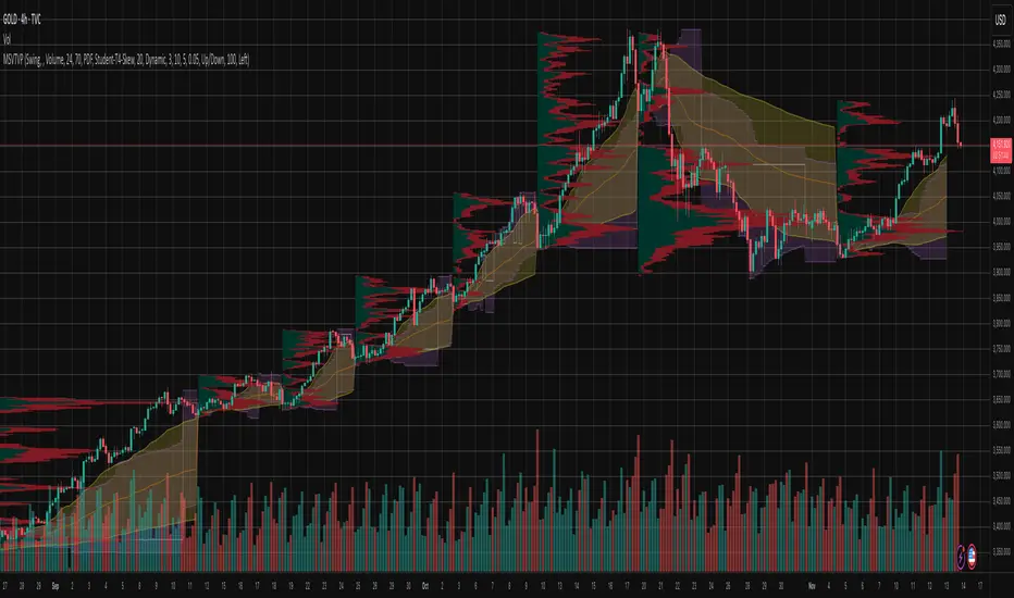
Market Structure Volume Time Velocity ProfileThis is the Market Structure Volume Time Velocity Profile (MSVTVP). It combines event-based profiling with advanced metrics like Time and Velocity (Flow Rate). Instead of fixed time periods, profiles are anchored to critical market events (Swings, Structure Breaks, Delta Breaks), giving you a precise view of value development during specific market phases.
## The 3 Dimensions of the Market
Unlike standard tools that only show Volume, MSVTVP allows you
to switch between three critical metrics:
1. **VOLUME Profile (The "Where"):**
* Shows standard acceptance. High volume nodes (HVN)
are magnets for price.
2. **TIME Profile (The "How Long"):**
* Similar to TPO, it measures how long price spent at each
level.
* **High Time:** True acceptance and fair value.
* **Low Time:** Rejection or rapid movement.
3. **VELOCITY Profile (The "How Fast"):**
* Measures the **speed of trading** (Contracts per Second).
This reveals the hidden intent of market participants.
* **High Velocity (Fast Flow):** Aggression. Initiative
buyers/sellers are hitting market orders rapidly. Often
seen at breakouts or in liquidity vacu.
* **Low Velocity (Slow Flow):** Absorption. Massive passive
limit orders are slowing price down despite high volume.
Often seen at major reversals ("hitting a brick wall").
Key Features:
1. **Event-Based Profile Anchoring:** The indicator starts a new
profile based on one of three user-selected events
('Profile Anchor'):
- **Swing:** A new profile begins when the 'impulse baseline'
(derived from intra-bar delta) changes. This baseline
adjusts when a new **price pivot** is confirmed: When a
price **high** forms, the baseline moves to the **lower**
of its previous level or the peak delta (max of
delta O/C) at the pivot. When a price **low** forms, it
moves to the **higher** of its previous level or the
trough delta (min of delta O/C) at the pivot.
- **Structure:** A new profile begins immediately on the bar
that *confirms* a market structure break (e.g., a new HH
or LL, based on a sequence of price pivots).
- **Delta:** A new profile begins immediately on the bar
that *confirms* a break in the *cumulative delta's*
market structure (e.g., a new HH or LL in the delta).
Both 'Swing' and 'Delta' anchors are derived from the same
**continuous (non-resetting) Cumulative Volume Profile Delta (CVPD)**,
which is built from the intra-bar statistical analysis.
2. **Statistical Profile Engine:** For each bar in the anchored
period, the indicator builds a volume profile on a lower
'Intra-Bar Timeframe'. Instead of simple tick counting, it
uses advanced statistical models:
- **Allocation ('Allot model'):** 'PDF' (Probability Density
Function) distributes volume proportionally across the
bar's range based on an assumed statistical model
(e.g., T4-Skew). 'Classic' assigns all volume to
the close.
- **Buy/Sell Split ('Volume Estimator'):** 'Dynamic'
applies a model that analyzes candle wicks and
recent trend to estimate buy/sell pressure. 'Classic'
classifies all volume based on the candle color.
3. **Visualization & Lag:** The indicator plots the final
profile (as a polygon) and the developing statistical
lines (POC, VA, VWAP, StdDev).
- **Note on Lag:** All anchor events require `Pivot Right Bars`
for confirmation.
- In 'Structure' and 'Delta' mode, the developing lines
(POC, VA, etc.) are plotted using a **non-repainting**
method (showing the value from `pivRi` bars ago).
- In 'Swing' mode, the profile is plotted **retroactively**,
starting *from the bar where the pivot occurred*. The
developing lines are also plotted with this full
`pivRi` lag to align with the past data.
4. **Flexible Display Modes:** The finalized profile can be displayed
in three ways: 'Up/Down' (buy vs. sell), 'Total' (combined
volume), and 'Delta' (net difference).
5. **Dynamic Row Sizing:** Includes an option ('Rows per Percent')
to automatically adjust the number of profile rows (buckets)
based on the profile's price range.
6. **Integrated Alerts:** Includes 13 alerts that trigger for:
- A new profile reset ('Profile was resetted').
- Price crossing any of the 6 developing levels (POC,
VA High/Low, VWAP, StdDev High/Low).
- **Alert Lag Assumption:** In 'Swing' mode, alerts are
delayed to match the retroactively plotted lines.
In 'Structure' and 'Delta' modes, alerts fire in
**real-time** based on the *current price* crossing
the *current (repainting)* value of the metric, which
may **differ from the non-repainting plotted line.**
**Caution: Real-Time Data Behavior (Intra-Bar Repainting)**
This indicator uses high-resolution intra-bar data. As a result, the
values on the **current, unclosed bar** (the real-time bar) will
update dynamically as new intra-bar data arrives. This includes
the values used for real-time alerts in 'Structure' and
'Delta' modes.
---
**DISCLAIMER**
1. **For Informational/Educational Use Only:** This indicator is
provided for informational and educational purposes only. It does
not constitute financial, investment, or trading advice, nor is
it a recommendation to buy or sell any asset.
2. **Use at Your Own Risk:** All trading decisions you make based on
the information or signals generated by this indicator are made
solely at your own risk.
3. **No Guarantee of Performance:** Past performance is not an
indicator of future results. The author makes no guarantee
regarding the accuracy of the signals or future profitability.
4. **No Liability:** The author shall not be held liable for any
financial losses or damages incurred directly or indirectly from
the use of this indicator.
5. **Signals Are Not Recommendations:** The alerts and visual signals
(e.g., crossovers) generated by this tool are not direct
recommendations to buy or sell. They are technical observations
for your own analysis and consideration.
Periodic Volume Time Velocity ProfileThis is the Periodic Volume Time Velocity Profile (PVTVP). It is an advanced professional profiling tool that goes beyond standard volume analysis by introducing Time and Velocity (Flow Rate) as profile dimensions.
By analyzing high-resolution intra-bar data, it builds
precise profiles for any custom period (Session, Day, Week, etc.),
helping you understand not just *where* the market traded,
but *how* it traded there.
## The 3 Dimensions of the Market
Unlike standard tools that only show Volume, PVTVP allows you
to switch between three critical metrics:
1. **VOLUME Profile (The "Where"):**
* Shows standard acceptance. High volume nodes (HVN)
are magnets for price.
2. **TIME Profile (The "How Long"):**
* Similar to TPO, it measures how long price spent at each
level.
* **High Time:** True acceptance and fair value.
* **Low Time:** Rejection or rapid movement.
3. **VELOCITY Profile (The "How Fast"):**
* Measures the **speed of trading** (Contracts per Second).
This reveals the hidden intent of market participants.
* **High Velocity (Fast Flow):** Aggression. Initiative
buyers/sellers are hitting market orders rapidly. Often
seen at breakouts or in liquidity vacuums.
* **Low Velocity (Slow Flow):** Absorption. Massive passive
limit orders are slowing price down despite high volume.
Often seen at major reversals ("hitting a brick wall").
## Key Features
1. **Statistical Volume Profile Engine:** For each bar in the selected
period, the indicator builds a complete volume profile on a lower
'Intra-Bar Timeframe'. Instead of simple tick counting, it uses
**statistical models ('PDF' allocation)** to distribute volume
across price levels and **advanced classifiers ('Dynamic' split)**
to determine the buy/sell pressure within that profile.
2. **Flexible Profile Display:** The **finalized profile** (plotted at
the end of each period) can be visualized in three distinct
ways: 'Up/Down' (buy vs. sell), 'Total' (combined volume),
and 'Delta' (net difference).
3. **Developing Key Levels:** The indicator also plots the developing
Point of Control (POC), Value Area (VA), VWAP, and Standard
Deviation bands in real-time as the period unfolds, providing
live insights into the emerging market structure.
4. **Dynamic Row Sizing:** Includes an option ('Rows per Percent')
to automatically adjust the number of profile rows (buckets)
based on the profile's price range, maintaining a consistent
visual density.
5. **Integrated Alerts:** Includes 12 alerts that trigger when the
main price crosses over or under the key developing levels:
POC, VWAP, Value Area High/Low, and the +/- Standard
Deviation bands.
**Caution: Real-Time Data Behavior (Intra-Bar Repainting)**
This indicator uses high-resolution intra-bar data. As a result, the
values on the **current, unclosed bar** (the real-time bar) will
update dynamically as new intra-bar data arrives. This behavior is
normal and necessary for this type of analysis. Signals should only
be considered final **after the main chart bar has closed.**
---
**DISCLAIMER**
1. **For Informational/Educational Use Only:** This indicator is
provided for informational and educational purposes only. It does
not constitute financial, investment, or trading advice, nor is
it a recommendation to buy or sell any asset.
2. **Use at Your Own Risk:** All trading decisions you make based on
the information or signals generated by this indicator are made
solely at your own risk.
3. **No Guarantee of Performance:** Past performance is not an
indicator of future results. The author makes no guarantee
regarding the accuracy of the signals or future profitability.
4. **No Liability:** The author shall not be held liable for any
financial losses or damages incurred directly or indirectly from
the use of this indicator.
5. **Signals Are Not Recommendations:** The alerts and visual signals
(e.g., crossovers) generated by this tool are not direct
recommendations to buy or sell. They are technical observations
for your own analysis and consideration.

Intra Bar Volume ProfileThis indicator provides a high-resolution volume profile analysis for every single bar on the chart. It builds this profile by sampling data from a lower intra-bar timeframe, allowing for a granular view of price distribution and buying/selling pressure within the bar.
Key Features:
Intra-Bar Profile Engine: For each bar on the main chart, the indicator builds a complete volume profile on a lower 'Intra-Bar Timeframe'. It uses:
Statistical Models ('Allot model'): Distributes volume across price levels using 'PDF' (Probability Density Function) or 'Classic' (close) methods.
Buy/Sell Classifiers ('Volume Estimator'): Splits volume using a 'Dynamic' (trend/wick-based) or 'Classic' (candle color) model.
On-Chart Visualization (Overlay): The analysis is rendered directly onto the price bars:
Point of Control (POC): A line showing the price level with the most volume for that bar.
Value Area (VA): A colored box representing the price range where the specified percentage (e..g., 50%) of volume was traded.
VWAP: Displays the volume-weighted average price (VWAP) for the bar as a separate line.
Integrated Alerts: Includes 8 alerts that trigger when the main price crosses over or under the key intra-bar levels: POC, VWAP, and the Value Area High/Low.
Caution: Real-Time Data Behavior (Intra-Bar Repainting) This indicator uses high-resolution intra-bar data. As a result, the values on the current, unclosed bar (the real-time bar) will update dynamically as new intra-bar data arrives. This behavior is normal and necessary for this type of analysis. Signals should only be considered final after the main chart bar has closed.
DISCLAIMM
For Informational/Educational Use Only: This indicator is provided for informational and educational purposes only. It does not constitute financial, investment, or trading advice, nor is it a recommendation to buy or sell any asset.
Use at Your Own Risk: All trading decisions you make based on the information or signals generated by this indicator are made solely at your own risk.
No Guarantee of Performance: Past performance is not an indicator of future results. The author makes no guarantee regarding the accuracy of the signals or future profitability.
No Liability: The author shall not be held liable for any financial losses or damages incurred directly or indirectly from the use of this indicator.
Signals Are Not Recommendations: The alerts and visual signals (e.g., crossovers) generated by this tool are not direct recommendations to buy or sell. They are technical observations for your own analysis and consideration.

Market Structure Volume ProfileThis indicator visualizes volume profiles that are dynamically anchored to market structure events, rather than fixed time intervals. It builds these profiles using high-resolution intra-bar data to provide a precise view of where value is established during critical market phases.
Key Features:
Event-Based Profile Anchoring: The indicator starts a new profile based on one of three user-selected events ('Profile Anchor'):
Swing: A new profile begins when the 'impulse baseline' (derived from intra-bar delta) changes. This baseline adjusts when a new price pivot is confirmed: When a price high forms, the baseline moves to the lower of its previous level or the peak delta (max of delta O/C) at the pivot. When a price low forms, it moves to the higher of its previous level or the trough delta (min of delta O/C) at the pivot.
Structure: A new profile begins immediately on the bar that confirms a market structure break (e.g., a new HH or LL, based on a sequence of price pivots).
Delta: A new profile begins immediately on the bar that confirms a break in the cumulative delta's market structure (e.g., a new HH or LL in the delta). Both 'Swing' and 'Delta' anchors are derived from the same continuous (non-resetting) Cumulative Volume Profile Delta (CVPD), which is built from the intra-bar statistical analysis.
Statistical Profile Engine: For each bar in the anchored period, the indicator builds a volume profile on a lower 'Intra-Bar Timeframe'. Instead of simple tick counting, it uses advanced statistical models:
Allocation ('Allot model'): 'PDF' (Probability Density Function) distributes volume proportionally across the bar's range based on an assumed statistical model (e.g., T4-Skew). 'Classic' assigns all volume to the close.
Buy/Sell Split ('Volume Estimator'): 'Dynamic' applies a model that analyzes candle wicks and recent trend to estimate buy/sell pressure. 'Classic' classifies all volume based on the candle color.
Visualization & Lag: The indicator plots the final profile (as a polygon) and the developing statistical lines (POC, VA, VWAP, StdDev).
Note on Lag: All anchor events require Pivot Right Bars for confirmation.
In 'Structure' and 'Delta' mode, the developing lines (POC, VA, etc.) are plotted using a non-repainting method (showing the value from pivRi bars ago).
In 'Swing' mode, the profile is plotted retroactively, starting from the bar where the pivot occurred. The developing lines are also plotted with this full pivRi lag to align with the past data.
Flexible Display Modes: The finalized profile can be displayed in three ways: 'Up/Down' (buy vs. sell), 'Total' (combined volume), and 'Delta' (net difference).
Dynamic Row Sizing: Includes an option ('Rows per Percent') to automatically adjust the number of profile rows (buckets) based on the profile's price range.
Integrated Alerts: Includes 13 alerts that trigger for:
A new profile reset ('Profile was resetted').
Price crossing any of the 6 developing levels (POC, VA High/Low, VWAP, StdDev High/Low).
Alert Lag Assumption: In 'Swing' mode, alerts are delayed to match the retroactively plotted lines. In 'Structure' and 'Delta' modes, alerts fire in real-time based on the current price crossing the current (repainting) value of the metric, which may differ from the non-repainting plotted line.
Caution: Real-Time Data Behavior (Intra-Bar Repainting) This indicator uses high-resolution intra-bar data. As a result, the values on the current, unclosed bar (the real-time bar) will update dynamically as new intra-bar data arrives. This includes the values used for real-time alerts in 'Structure' and 'Delta' modes.
DISCLAIMER
For Informational/Educational Use Only: This indicator is provided for informational and educational purposes only. It does not constitute financial, investment, or trading advice, nor is it a recommendation to buy or sell any asset.
Use at Your Own Risk: All trading decisions you make based on the information or signals generated by this indicator are made solely at your own risk.
No Guarantee of Performance: Past performance is not an indicator of future results. The author makes no guarantee regarding the accuracy of the signals or future profitability.
No Liability: The author shall not be held liable for any financial losses or damages incurred directly or indirectly from the use of this indicator.
Signals Are Not Recommendations: The alerts and visual signals (e.g., crossovers) generated by this tool are not direct recommendations to buy or sell. They are technical observations for your own analysis and consideration.

Periodic Volume ProfileThis indicator visualizes volume profiles that are dynamically anchored to market structure events, rather than fixed time intervals. It builds these profiles using high-resolution intra-bar data to provide a precise view of where value is established during critical market phases.
Key Features:
Event-Based Profile Anchoring: The indicator starts a new profile based on one of three user-selected events ('Profile Anchor'):
Swing: A new profile begins when the 'impulse baseline' (derived from delta) changes. This baseline adjusts when a new price pivot is confirmed: When a price high forms, the baseline moves to the lower of its previous level or the peak delta (max of delta O/C) at the pivot. When a price low forms, it moves to the higher of its previous level or the trough delta (min of delta O/C).
Structure: A new profile begins immediately on the bar that confirms a market structure break (e.g., a new HH or LL, based on a sequence of price pivots).
Delta: A new profile begins immediately on the bar that confirms a break in the cumulative delta's market structure (e.g., a new HH or LL in the delta).
Statistical Profile Engine: For each bar in the anchored period, the indicator builds a volume profile on a lower 'Intra-Bar Timeframe'. It uses:
Statistical Models ('Allot model'): Distributes volume across price levels using 'PDF' (Probability Density Function) or 'Classic' (close) methods.
Buy/Sell Classifiers ('Volume Estimator'): Splits volume using a 'Dynamic' (trend/wick-based) or 'Classic' (candle color) model.
Note on Anchor Lag: The different anchor types have different delays. 'Structure' and 'Delta' profiles begin in real-time on the confirmation bar. The 'Swing' profile calculation is plotted retroactively to the pivot's origin, as the pivot is only confirmed Pivot Right Bars after it occurs.
Flexible Visualization Modes: The finalized profile (plotted at the end of each period) can be displayed in three ways: 'Up/Down' (buy vs. sell), 'Total' (combined volume), and 'Delta' (net difference).
Developing Real-Time Metrics: The indicator plots the developing Point of Control (POC), Value Area (VA), VWAP, and Standard Deviation bands in real-time as the new profile forms.
Dynamic Row Sizing: Includes an option ('Rows per Percent') to automatically adjust the number of profile rows (buckets) based on the profile's price range, maintaining a consistent visual density.
Integrated Alerts: Includes 13 alerts that trigger for:
A new profile reset ('Profile was resetted').
Price crossing any of the 6 developing levels (POC, VA High/Low, VWAP, StdDev High/Low).
Caution: Real-Time Data Behavior (Intra-Bar Repainting) This indicator uses high-resolution intra-bar data. As a result, the values on the current, unclosed bar (the real-time bar) will update dynamically as new intra-bar data arrives. This behavior is normal and necessary for this type of analysis. Signals should only be considered final after the main chart bar has closed.
DISCLAIMER
For Informational/Educational Use Only: This indicator is provided for informational and educational purposes only. It does not constitute financial, investment, or trading advice, nor is it a recommendation to buy or sell any asset.
Use at Your Own Risk: All trading decisions you make based on the information or signals generated by this indicator are made solely at your own risk.
No Guarantee of Performance: Past performance is not an indicator of future results. The author makes no guarantee regarding the accuracy of the signals or future profitability.
No Liability: The author shall not be held liable for any financial losses or damages incurred directly or indirectly from the use of this indicator.
Signals Are Not Recommendations: The alerts and visual signals (e.g., crossovers) generated by this tool are not direct recommendations to buy or sell. They are technical observations for your own analysis and consideration.
Pivot Orderflow DeltaThis indicator analyzes order flow by calculating a continuous Cumulative Volume Profile Delta (CVPD). It plots this delta as a series of "delta candles" and identifies divergences and structural pivot levels.
Key Features:
Statistical Delta Engine: For each bar, the indicator builds a high-resolution volume profile on a lower 'Intra-Bar Timeframe'. It uses statistical models ('PDF' allocation) and advanced classifiers ('Dynamic' split) to determine the buy/sell pressure, which is then accumulated.
Cumulative Delta Candle Visualization: The indicator plots the continuous, accumulated delta as a series of candles, where for each bar:
Open: Is the cumulative delta value of the previous bar.
Close: Is the new total cumulative delta.
High/Low: Represent the peak/trough cumulative delta reached during that bar's formation.
Dynamic Pivot Baseline: The indicator plots a separate dynamic baseline ('Impulse Start') that adjusts when a new price pivot is confirmed.
When a price high forms, the baseline moves to the lower of its previous level or the peak delta (max of delta candle O/C) at the pivot.
When a price low forms, the baseline moves to the higher of its previous level or the trough delta (min of delta candle O/C) at the pivot.
Full Divergence Suite (Class A, B, C): A built-in divergence engine automatically detects and plots Regular (A), Hidden (B), and Exaggerated (C) divergences between price and the peak/trough of the delta candles (High/Low).
Detailed Pivot Confluence: The indicator plots distinct markers to differentiate between pivots occurring only on the price chart, only on the delta oscillator, or on both simultaneously.
Note on Confirmation (Lag): Divergence and pivot signals rely on a confirmation method. A pivot is only plotted after the Pivot Right Bars input has passed, which introduces an inherent lag.
Integrated Alerts: Includes 23 comprehensive alerts for:
The start and end of all 6 divergence types.
The detection of a new Impulse Start pivot.
Delta/volume agreement/disagreement.
Delta crossing the zero line.
The formation of price-only or delta-only pivots.
Caution: Real-Time Data Behavior (Intra-Bar Repainting) This indicator uses high-resolution intra-bar data. As a result, the values on the current, unclosed bar (the real-time bar) will update dynamically as new intra-bar data arrives. This behavior is normal and necessary for this type of analysis. Signals should only be considered final after the main chart bar has closed.
DISCLAIMER
For Informational/Educational Use Only: This indicator is provided for informational and educational purposes only. It does not constitute financial, investment, or trading advice, nor is it a recommendation to buy or sell any asset.
Use at Your Own Risk: All trading decisions you make based on the information or signals generated by this indicator are made solely at your own risk.
No Guarantee of Performance: Past performance is not an indicator of future results. The author makes no guarantee regarding the accuracy of the signals or future profitability.
No Liability: The author shall not be held liable for any financial losses or damages incurred directly or indirectly from the use of this indicator.
Signals Are Not Recommendations: The alerts and visual signals (e.g., crossovers) generated by this tool are not direct recommendations to buy or sell. They are technical observations for your own analysis and consideration.

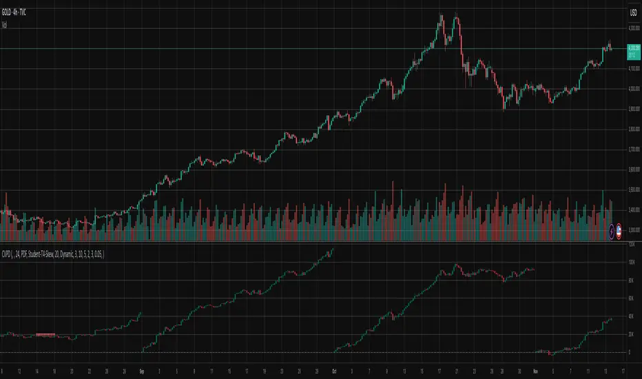
Cumulative Volume Profile DeltaThis indicator calculates the Cumulative Volume Profile Delta (CVPD). It constructs a high-resolution volume profile for each bar using intra-bar data, then derives and accumulates the delta from that profile to show net buying/selling pressure.
Key Features:
Statistical Volume Profile Engine: For each bar, the indicator builds a high-resolution volume profile on a lower 'Intra-Bar Timeframe'. Instead of simple tick counting, it uses statistical models ('PDF' allocation) to distribute volume across price levels and advanced classifiers ('Dynamic' split) to determine the buy/sell pressure before accumulation.
Periodic Accumulation: The CVPD accumulation is anchored to a user-defined 'Anchor Timeframe' (e.g., daily, weekly). This cyclical reset allows to analyze the build-up of pressure within specific trading periods.
"Delta Candle" Visualization: The periodic CVPD is shown as a candle, where:
Open: The CVPD value at the start of the period (or zero).
High/Low: Represent the peak buying (CVD High) and selling (CVD Low) pressure within that period's profile.
Close: The final net delta value (CVD) for the period.
Dual CVD & Divergence Engine: The indicator calculates two CVPDs: a Periodic one (for plotting) and a Continuous one (non-resetting). The continuous line is used as a stable source for the built-in divergence engine (detecting Regular, Hidden, and Exaggerated).
Dynamic Divergence Plotting: Divergence markers are plotted relative to the periodic (candle) CVPD. They automatically adjust their vertical position after a reset to remain visually aligned with the plotted candles.
Note on Confirmation (Lag): Divergence signals rely on a pivot confirmation method to ensure they do not repaint.
The Start of a- divergence is only detected after the confirming pivot is fully formed (a delay based on Pivot Right Bars).
The End of a divergence is detected either instantly (if the signal is invalidated by price action) or with a delay (when a new, non-divergent pivot is confirmed).
Multi-Timeframe (MTF) Capability:
MTF Output: The entire analysis (Delta Candles, Divergences) can be calculated on a higher timeframe (using the Timeframe input), with standard options to handle gaps (Fill Gaps) and prevent repainting (Wait for...).
Limitation: The Divergence detection engine (pivDiv) is disabled if a Higher Timeframe (HTF) is selected.
Integrated Alerts: Includes 18 comprehensive alerts for:
The start and end of all 6 divergence types.
The periodic CVPD crossing the zero line.
Conditions of agreement or disagreement between the delta and the main bar's direction.
Caution: Real-Time Data Behavior (Intra-Bar Repainting) This indicator uses high-resolution intra-bar data. As a result, the values on the current, unclosed bar (the real-time bar) will update dynamically as new intra-bar data arrives. This behavior is normal and necessary for this type of analysis. Signals should only be considered final after the main chart bar has closed.
DISCLAIMER
For Informational/Educational Use Only: This indicator is provided for informational and educational purposes only. It does not constitute financial, investment, or trading advice, nor is it a recommendation to buy or sell any asset.
Use at Your Own Risk: All trading decisions you make based on the information or signals generated by this indicator are made solely at your own risk.
No Guarantee of Performance: Past performance is not an indicator of future results. The author makes no guarantee regarding the accuracy of the signals or future profitability.
No Liability: The author shall not be held liable for any financial losses or damages incurred directly or indirectly from the use of this indicator.
Signals Are Not Recommendations: The alerts and visual signals (e.Example: crossovers) generated by this tool are not direct recommendations to buy or sell. They are technical observations for your own analysis and consideration.
Volume Profile DeltaThis indicator calculates the Volume Profile Delta (VPD). It constructs a high-resolution volume profile for each bar using intra-bar data, offering a detailed understanding of buying and selling pressure at discrete price levels.
Key Features:
Statistical Volume Profile Engine: For each bar, the indicator builds a high-resolution volume profile on a lower 'Intra-Bar Timeframe'. Instead of simple tick counting, it uses statistical models ('PDF' allocation) to distribute volume across price levels and advanced classifiers ('Dynamic' split) to determine the buy/sell pressure within that profile, providing a more nuanced delta calculation.
"Delta Candle" Visualization: The per-bar VPD is displayed as a candle, where:
Open: Always anchored at the zero line.
High/Low: Represent the peak buying (CVD High) and selling (CVD Low) pressure accumulated within that bar's profile.
Close: The final net delta value (CVD) for the bar.
Customizable Moving Average: An optional moving average of the net delta (Close) can be added. The MA type, length, and an optional Volume weighted setting are customizable.
Intra-Bar Peak Pivot Detection: Automatically identifies and plots significant turning points (pivots) in the peak buying (High) and selling (Low) pressure.
Note on Confirmation (Lag): Pivot signals are confirmed using a lookback method. A pivot is only plotted after the Pivot Right Bars input has passed, which introduces an inherent lag.
Multi-Timeframe (MTF) Capability:
MTF Output: The entire analysis (Delta Candles, MA, Pivots) can be calculated on a higher timeframe (using the Timeframe input), with standard options to handle gaps (Fill Gaps) and prevent repainting (Wait for...).
Limitation: The Pivot detection (Calculate Pivots) is disabled if a Higher Timeframe (HTF) is selected.
Integrated Alerts: Includes 8 alerts for:
The net delta crossing its moving average.
The detection of new peak buying or selling pivots.
Conditions of agreement or disagreement between the net delta and the main bar's direction.
Caution: Real-Time Data Behavior (Intra-Bar Repainting) This indicator uses high-resolution intra-bar data. As a result, the values on the current, unclosed bar (the real-time bar) will update dynamically as new intra-bar data arrives. This behavior is normal and necessary for this type of analysis. Signals should only be considered final after the main chart bar has closed.
DISCLAIMER
For Informational/Educational Use Only: This indicator is provided for informational and educational purposes only. It does not constitute financial, investment, or trading advice, nor is it a recommendation to buy or sell any asset.
Use at Your Own Risk: All trading decisions you make based on the information or signals generated by this indicator are made solely at your own risk.
No Guarantee of Performance: Past performance is not an indicator of future results. The author makes no guarantee regarding the accuracy of the signals or future profitability.
No Liability: The author shall not be held liable for any financial losses or damages incurred directly or indirectly from the use of this indicator.
Signals Are Not Recommendations: The alerts and visual signals (e.g., crossovers) generated by this tool are not direct recommendations to buy or sell. They are technical observations for your own analysis and consideration.

LibBrStLibrary "LibBrSt"
This is a library for quantitative analysis, designed to estimate
the statistical properties of price movements *within* a single
OHLC bar, without requiring access to tick data. It provides a
suite of estimators based on various statistical and econometric
models, allowing for analysis of intra-bar volatility and
price distribution.
Key Capabilities:
1. **Price Distribution Models (`PriceEst`):** Provides a selection
of estimators that model intra-bar price action as a probability
distribution over the range. This allows for the
calculation of the intra-bar mean (`priceMean`) and standard
deviation (`priceStdDev`) in absolute price units. Models include:
- **Symmetric Models:** `uniform`, `triangular`, `arcsine`,
`betaSym`, and `t4Sym` (Student-t with fat tails).
- **Skewed Models:** `betaSkew` and `t4Skew`, which adjust
their shape based on the Open/Close position.
- **Model Assumptions:** The skewed models rely on specific
internal constants. `betaSkew` uses a fixed concentration
parameter (`BETA_SKEW_CONCENTRATION = 4.0`), and `t4Sym`/`t4Skew`
use a heuristic scaling factor (`T4_SHAPE_FACTOR`)
to map the distribution.
2. **Econometric Log-Return Estimators (`LogEst`):** Includes a set of
econometric estimators for calculating the volatility (`logStdDev`)
and drift (`logMean`) of logarithmic returns within a single bar.
These are unit-less measures. Models include:
- **Parkinson (1980):** A High-Low range estimator.
- **Garman-Klass (1980):** An OHLC-based estimator.
- **Rogers-Satchell (1991):** An OHLC estimator that accounts
for non-zero drift.
3. **Distribution Analysis (PDF/CDF):** Provides functions to work
with the Probability Density Function (`pricePdf`) and
Cumulative Distribution Function (`priceCdf`) of the
chosen price model.
- **Note on `priceCdf`:** This function uses analytical (exact)
calculations for the `uniform`, `triangular`, and `arcsine`
models. For all other models (e.g., `betaSkew`, `t4Skew`),
it uses **numerical integration (Simpson's rule)** as
an approximation of the cumulative probability.
4. **Mathematical Functions:** The library's Beta distribution
models (`betaSym`, `betaSkew`) are supported by an internal
implementation of the natural log-gamma function, which is
based on the Lanczos approximation.
---
**DISCLAIMER**
This library is provided "AS IS" and for informational and
educational purposes only. It does not constitute financial,
investment, or trading advice.
The author assumes no liability for any errors, inaccuracies,
or omissions in the code. Using this library to build
trading indicators or strategies is entirely at your own risk.
As a developer using this library, you are solely responsible
for the rigorous testing, validation, and performance of any
scripts you create based on these functions. The author shall
not be held liable for any financial losses incurred directly
or indirectly from the use of this library or any scripts
derived from it.
priceStdDev(estimator, offset)
Estimates **σ̂** (standard deviation) *in price units* for the current
bar, according to the chosen `PriceEst` distribution assumption.
Parameters:
estimator (series PriceEst) : series PriceEst Distribution assumption (see enum).
offset (int) : series int To offset the calculated bar
Returns: series float σ̂ ≥ 0 ; `na` if undefined (e.g. zero range).
priceMean(estimator, offset)
Estimates **μ̂** (mean price) for the chosen `PriceEst` within the
current bar.
Parameters:
estimator (series PriceEst) : series PriceEst Distribution assumption (see enum).
offset (int) : series int To offset the calculated bar
Returns: series float μ̂ in price units.
pricePdf(estimator, price, offset)
Probability-density under the chosen `PriceEst` model.
**Returns 0** when `p` is outside the current bar’s .
Parameters:
estimator (series PriceEst) : series PriceEst Distribution assumption (see enum).
price (float) : series float Price level to evaluate.
offset (int) : series int To offset the calculated bar
Returns: series float Density value.
priceCdf(estimator, upper, lower, steps, offset)
Cumulative probability **between** `upper` and `lower` under
the chosen `PriceEst` model. Outside-bar regions contribute zero.
Uses a fast, analytical calculation for Uniform, Triangular, and
Arcsine distributions, and defaults to numerical integration
(Simpson's rule) for more complex models.
Parameters:
estimator (series PriceEst) : series PriceEst Distribution assumption (see enum).
upper (float) : series float Upper Integration Boundary.
lower (float) : series float Lower Integration Boundary.
steps (int) : series int # of sub-intervals for numerical integration (if used).
offset (int) : series int To offset the calculated bar.
Returns: series float Probability mass ∈ .
logStdDev(estimator, offset)
Estimates **σ̂** (standard deviation) of *log-returns* for the current bar.
Parameters:
estimator (series LogEst) : series LogEst Distribution assumption (see enum).
offset (int) : series int To offset the calculated bar
Returns: series float σ̂ (unit-less); `na` if undefined.
logMean(estimator, offset)
Estimates μ̂ (mean log-return / drift) for the chosen `LogEst`.
The returned value is consistent with the assumptions of the
selected volatility estimator.
Parameters:
estimator (series LogEst) : series LogEst Distribution assumption (see enum).
offset (int) : series int To offset the calculated bar
Returns: series float μ̂ (unit-less log-return).
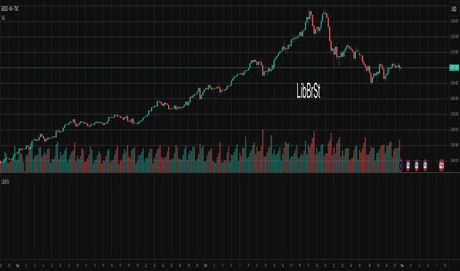
Likelihood of Winning - Probability Density FunctionIn developing the "Likelihood of Winning - Probability Density Function (PDF)" indicator, my aim was to offer traders a statistical tool to quantify the probability of reaching target prices. This indicator, grounded in risk assessment principles, enables users to analyze potential outcomes based on the normal distribution, providing insights into market dynamics.
The tool's flexibility allows for customization of the data series, lookback periods, and target settings for both long and short scenarios. It features a color-coded visualization to easily distinguish between probabilities of hitting specified targets, enhancing decision-making in trading strategies.
I'm excited to share this indicator with the trading community, hoping it will enhance data-driven decision-making and offer a deeper understanding of market risks and opportunities. My goal is to continuously improve this tool based on user feedback and market evolution, contributing to more informed trading practices.
This indicator leverages the "NormalDistributionFunctions" library, enabling easy integration into other indicators or strategies. Users can readily embed advanced statistical analysis into their trading tools, fostering innovation within the Pine Script community.
Stress DashboardEnglish:
The Stress Dashboard is based on the Kansas City Financial Stress Index. In most general terms, financial stress can be thought of as an interruption to the normal functioning of financial markets.
For more information about the Stress index read the pdf from kansascityfed.org:
www.kansascityfed.org
If the value is above 0 it indicates that financial stress is above the long-run average, while a value below 0 signifies that financial stress is below the long-run average.
You can use it as a early warning system to bigger down moves or possible crashes and left the market early.
I use it in combine with my Volatility Dashboard as my own early warning system because the Stess Index only get updated monthly so that the Volatility Dashboard warning me much faster.
I dont want to have only one crash indicator so I search for another and found these. If you transfer the red areas of the indicator into the S&P 500 Chart then you can see how good these Dashboard warning you for a following crash/ downtrend/ bigger correction.
Deutsch:
Das Stress Dashboard basiert auf dem Kansas City Financial Stress Index. Finanzielle Belastungen können im Allgemeinen als Unterbrechung des normalen Funktionierens der Finanzmärkte angesehen werden.
Weitere Informationen zum Stress-Index finden Sie im PDF von kansascityfed.org:
www.kansascityfed.org
Wenn der Wert über 0 liegt bedeutet dies, dass die finanzielle Belastung über dem langfristigen Durchschnitt liegt, während ein Wert unter 0 bedeutet, dass die finanzielle Belastung unter dem langfristigen Durchschnitt liegt.
Sie können es als Frühwarnsystem für größere Abwärtsbewegungen oder mögliche Abstürze verwenden und den Markt frühzeitig verlassen.
Ich verwende es in Kombination mit meinem Volatility Dashboard als mein eigenes Frühwarnsystem, da der Stess-Index nur monatlich aktualisiert wird, sodass mich das Volatility Dashboard viel schneller warnt.
Ich möchte nicht nur einen Crash Indikator haben, also suchte ich nach einer weiteren und fand diesen. Wenn Sie die roten Bereiche des Indikators in den S&P 500 Chart übertragen, können Sie sehen wie gut dieses Dashboard Sie vor einem folgenden Absturz / Abwärtstrend / einer größeren Korrektur warnt.

CauchyTrend [InvestorUnknown]The CauchyTrend is an experimental tool that leverages a Cauchy-weighted moving average combined with a modified Supertrend calculation. This unique approach provides traders with insight into trend direction, while also offering an optional ATR-based range analysis to understand how often the market closes within, above, or below a defined volatility band.
Core Concepts
Cauchy Distribution and Gamma Parameter
The Cauchy distribution is a probability distribution known for its heavy tails and lack of a defined mean or variance. It is characterized by two parameters: a location parameter (x0, often 0 in our usage) and a scale parameter (γ, "gamma").
Gamma (γ): Determines the "width" or scale of the distribution. Smaller gamma values produce a distribution more concentrated near the center, giving more weight to recent data points, while larger gamma values spread the weight more evenly across the sample.
In this indicator, gamma influences how much emphasis is placed on values closer to the current price versus those further away in time. This makes the resulting weighted average either more reactive or smoother, depending on gamma’s value.
// Cauchy PDF formula used for weighting:
// f(x; γ) = (1/(π*γ)) *
f_cauchyPDF(offset, gamma) =>
numerator = gamma * gamma
denominator = (offset * offset) + (gamma * gamma)
pdf = (1 / (math.pi * gamma)) * (numerator / denominator)
pdf
A chart showing different Cauchy PDFs with various gamma values, illustrating how gamma affects the weight distribution.
Cauchy-Weighted Moving Average (CWMA)
Using the Cauchy PDF, we calculate normalized weights to create a custom Weighted Moving Average. Each bar in the lookback period receives a weight according to the Cauchy PDF. The result is a Cauchy Weighted Average (cwm_avg) that differs from typical moving averages, potentially offering unique sensitivity to price movements.
// Summation of weighted prices using Cauchy distribution weights
cwm_avg = 0.0
for i = 0 to length - 1
w_norm = array.get(weights, i) / sum_w
cwm_avg += array.get(values, i) * w_norm
Supertrend with a Cauchy Twist
The indicator integrates a modified Supertrend calculation using the cwm_avg as its reference point. The Supertrend logic typically sets upper and lower bands based on volatility (ATR), and flips direction when price crosses these bands.
In this case, the Cauchy-based average replaces the usual baseline, aiming to capture trend direction via a different weighting mechanism.
When price closes above the upper band, the trend is considered bullish; closing below the lower band signals a bearish trend.
ATR Stats Range (Optional)
Beyond the fundamental trend detection, the indicator optionally computes ATR-based stats to understand price distribution relative to a volatility corridor centered on the cwm_avg line:
Volatility Range:
Defined as cwm_avg ± (ATR * atr_mult), this range creates upper and lower bands. Turning on atr_stats computes how often the daily close falls: Within the range, Above the upper ATR boundary, Below the lower ATR boundary, Within the range but above cwm_avg, Within the range but below cwm_avg
These statistics can help traders gauge how the market behaves relative to this volatility envelope and possibly identify if the market tends to revert to the mean or break out more often.
Backtesting and Performance Metrics
The code is integrated with a backtesting library that allows users to assess strategy performance historically:
Equity Curve Calculation: Compares CauchyTrend-based signals against the underlying asset.
Performance Metrics Table: Once enabled, displays key metrics such as mean returns, Sharpe Ratio, Sortino Ratio, and more, comparing the strategy to a simple Buy & Hold approach.
Alerts and Notifications
The indicator provides Alerts for key events:
Long Alert: Triggered when the trend flips bullish.
Short Alert: Triggered when the trend flips bearish.
Customization and Calibration
Important: The default parameters are not optimized for any specific instrument or time frame. Traders should:
Adjust the length and gamma parameters to influence how sharply or broadly the cwm_avg reacts to price changes.
Tune the atr_len and atr_mult for the Supertrend logic to better match the asset’s volatility characteristics.
Experiment with atr_stats on/off to see if that additional volatility distribution information provides helpful insights.
Traders may find certain sets of parameters that align better with their preferred trading style, risk tolerance, or asset volatility profile.
Disclaimer: This indicator is for educational and informational purposes only. Past performance in backtesting does not guarantee future results. Always perform due diligence, and consider consulting a qualified financial advisor before trading.

CM Stochastic POP Method 2-Jake Bernstein_V1Yesterday Jake Bernstein authorized me to post his updated results with the Stochastic Pop Trading System he developed many years ago.
You can take a look at the Original System with Updated Settings at
This indicator is a different set of rules Jake mentioned in the PDF he allowed me to post.
To view the PDF use this link:
dl.dropboxusercontent.com
Today we’re releasing the version described in the PDF that uses the StochK values of 55, 50, and 45. The rules are discussed in the PDF but here is a simple breakdown:
Enter Long when StochK is below 50 and Crosses Above 55
Exit Long on Cross Below 55
Enter Short when StochK is Above 50 and crosses Below 45
Exit Short on Cross Above 45
Two Important Items to understand about this method:
To code the rules Precisely we need a function that will be available when Strategy Capabilities are released on TradingView.
There is one of Jakes Profit Maximizing Strategies that needs to be integrated with this code…which again we need the Strategy based Function that will be coming soon.
To Compare this system to the Stochastic Pop Method 1 System shown yesterday at I used the same Symbol and dates for you to compare…but remember to give this Method 2 System a Fair Look/Evaluation…we need the Soon To Be Released…TradingView Strategy Capabilities.
BackTesting Results Example: EUR-USD Daily Chart Since 01/01/2005
Strategy 1 – Stochastic Pop Method 2 System:
Go Long When Stochasticis below 50 and Crosses Above 55. Go Short When Stochastic is above 50 and Crosses Below 45. Exit Long/Short When Stochastic has a Reverse Cross of Entry Value.
Results:
Total Trades = 151
Profit = 40,758 Pips
Win% = 37.1%
Profit Factor = 1.26
Avg Trade = 270 Pips Profit
***Most Consecutive Wins = 4 ... Most Consecutive Losses = 7
Strategy 2:
Rules - Proprietary Optimization Jake Will Teach. Only Added 1 Additional Exit Rule.
Results:
Total Trades = 151
Profit = 60.305 Pips
Win% = 37.1%
Profit Factor = 1.38
Avg Trade = 399 Pips Profit
***Most Consecutive Wins = 4 ... Most Consecutive Losses = 7
Indicator Includes:
-Ability to Color Candles (CheckBox In Inputs Tab)
Green = Long Trade
Blue = No Trade
Red = Short Trade
Jake Bernstein will be a contributor on TradingView when Backtesting/Strategies are released. Jake is one of the Top Trading System Developers in the world with 45+ years experience and he is going to teach TradingView.com’s community how to create Trading Systems and how to Optimize the correct way.
Link To PDF:
dl.dropboxusercontent.com
Link to Original Version of Indicator with Updated Settings.

NormalDistributionFunctionsLibrary "NormalDistributionFunctions"
The NormalDistributionFunctions library encompasses a comprehensive suite of statistical tools for financial market analysis. It provides functions to calculate essential statistical measures such as mean, standard deviation, skewness, and kurtosis, alongside advanced functionalities for computing the probability density function (PDF), cumulative distribution function (CDF), Z-score, and confidence intervals. This library is designed to assist in the assessment of market volatility, distribution characteristics of asset returns, and risk management calculations, making it an invaluable resource for traders and financial analysts.
meanAndStdDev(source, length)
Calculates and returns the mean and standard deviation for a given data series over a specified period.
Parameters:
source (float) : float: The data series to analyze.
length (int) : int: The lookback period for the calculation.
Returns: Returns an array where the first element is the mean and the second element is the standard deviation of the data series for the given period.
skewness(source, mean, stdDev, length)
Calculates and returns skewness for a given data series over a specified period.
Parameters:
source (float) : float: The data series to analyze.
mean (float) : float: The mean of the distribution.
stdDev (float) : float: The standard deviation of the distribution.
length (int) : int: The lookback period for the calculation.
Returns: Returns skewness value
kurtosis(source, mean, stdDev, length)
Calculates and returns kurtosis for a given data series over a specified period.
Parameters:
source (float) : float: The data series to analyze.
mean (float) : float: The mean of the distribution.
stdDev (float) : float: The standard deviation of the distribution.
length (int) : int: The lookback period for the calculation.
Returns: Returns kurtosis value
pdf(x, mean, stdDev)
pdf: Calculates the probability density function for a given value within a normal distribution.
Parameters:
x (float) : float: The value to evaluate the PDF at.
mean (float) : float: The mean of the distribution.
stdDev (float) : float: The standard deviation of the distribution.
Returns: Returns the probability density function value for x.
cdf(x, mean, stdDev)
cdf: Calculates the cumulative distribution function for a given value within a normal distribution.
Parameters:
x (float) : float: The value to evaluate the CDF at.
mean (float) : float: The mean of the distribution.
stdDev (float) : float: The standard deviation of the distribution.
Returns: Returns the cumulative distribution function value for x.
confidenceInterval(mean, stdDev, size, confidenceLevel)
Calculates the confidence interval for a data series mean.
Parameters:
mean (float) : float: The mean of the data series.
stdDev (float) : float: The standard deviation of the data series.
size (int) : int: The sample size.
confidenceLevel (float) : float: The confidence level (e.g., 0.95 for 95% confidence).
Returns: Returns the lower and upper bounds of the confidence interval.
Inverse Fisher Transform on STOCHASTIC (modified graphics)Modified the graphic representation of the script from John Ehlers - From California, USA, he is a veteran trader. With 35 years trading experience he has seen it all. John has an engineering background that led to his technical approach to trading ignoring fundamental analysis (with one important exception). John strongly believes in cycles. He’d rather exit a trade when the cycle ends or a new one starts. He uses the MESA principle to make predictions about cycles in the market and trades one hundred percent automatically.
In the show John reveals:
• What is more appropriate than trading individual stocks
• The one thing he relies upon in his approach to the market
• The detail surrounding his unique trading style
• What important thing underpins the market and gives every trader an edge
About INVERSE FISHER TRANSFORM:
The purpose of technical indicators is to help with your timing decisions to buy or sell. Hopefully, the signals are clear and unequivocal. However, more often than not your decision to pull the trigger is accompanied by crossing your fingers. Even if you have placed only a few trades you know the drill. In this article I will show you a way to make your oscillator-type indicators make clear black-or-white indication of the time to buy or sell. I will do this by using the Inverse Fisher Transform to alter the Probability Distribution Function (PDF) of your indicators. In the past12 I have noted that the PDF of price and indicators do not have a Gaussian, or Normal, probability distribution. A Gaussian PDF is the familiar bell-shaped curve where the long “tails” mean that wide deviations from the mean occur with relatively low probability. The Fisher Transform can be applied to almost any normalized data set to make the resulting PDF nearly Gaussian, with the result that the turning points are sharply peaked and easy to identify. The Fisher Transform is defined by the equation
1)
Whereas the Fisher Transform is expansive, the Inverse Fisher Transform is compressive. The Inverse Fisher Transform is found by solving equation 1 for x in terms of y. The Inverse Fisher Transform is:
2)
The transfer response of the Inverse Fisher Transform is shown in Figure 1. If the input falls between –0.5 and +0.5, the output is nearly the same as the input. For larger absolute values (say, larger than 2), the output is compressed to be no larger than unity. The result of using the Inverse Fisher Transform is that the output has a very high probability of being either +1 or –1. This bipolar probability distribution makes the Inverse Fisher Transform ideal for generating an indicator that provides clear buy and sell signals.

Inverse Fisher Transform COMBO STO+RSI+CCIv2 by KIVANÇ fr3762A combined 3in1 version of pre shared INVERSE FISHER TRANSFORM indicators on RSI , on STOCHASTIC and on CCIv2 to provide space for 2 more indicators for users...
About John EHLERS:
From California, USA, John is a veteran trader. With 35 years trading experience he has seen it all. John has an engineering background that led to his technical approach to trading ignoring fundamental analysis (with one important exception).
John strongly believes in cycles. He’d rather exit a trade when the cycle ends or a new one starts. He uses the MESA principle to make predictions about cycles in the market and trades one hundred percent automatically.
In the show John reveals:
• What is more appropriate than trading individual stocks
• The one thing he relies upon in his approach to the market
• The detail surrounding his unique trading style
• What important thing underpins the market and gives every trader an edge
About INVERSE FISHER TRANSFORM:
The purpose of technical indicators is to help with your timing decisions to buy or
sell. Hopefully, the signals are clear and unequivocal. However, more often than
not your decision to pull the trigger is accompanied by crossing your fingers.
Even if you have placed only a few trades you know the drill.
In this article I will show you a way to make your oscillator-type indicators make
clear black-or-white indication of the time to buy or sell. I will do this by using the
Inverse Fisher Transform to alter the Probability Distribution Function ( PDF ) of
your indicators. In the past12 I have noted that the PDF of price and indicators do
not have a Gaussian, or Normal, probability distribution. A Gaussian PDF is the
familiar bell-shaped curve where the long “tails” mean that wide deviations from
the mean occur with relatively low probability. The Fisher Transform can be
applied to almost any normalized data set to make the resulting PDF nearly
Gaussian, with the result that the turning points are sharply peaked and easy to
identify. The Fisher Transform is defined by the equation
1)
Whereas the Fisher Transform is expansive, the Inverse Fisher Transform is
compressive. The Inverse Fisher Transform is found by solving equation 1 for x
in terms of y. The Inverse Fisher Transform is:
2)
The transfer response of the Inverse Fisher Transform is shown in Figure 1. If
the input falls between –0.5 and +0.5, the output is nearly the same as the input.
For larger absolute values (say, larger than 2), the output is compressed to be no
larger than unity . The result of using the Inverse Fisher Transform is that the
output has a very high probability of being either +1 or –1. This bipolar
probability distribution makes the Inverse Fisher Transform ideal for generating
an indicator that provides clear buy and sell signals.
Creator: John EHLERS
Inverse Fisher Transform on SMI (Stochastic Momentum Index)Inverse Fisher Transform on SMI (Stochastic Momentum Index)
About John EHLERS:
From California, USA, John is a veteran trader. With 35 years trading experience he has seen it all. John has an engineering background that led to his technical approach to trading ignoring fundamental analysis (with one important exception).
John strongly believes in cycles. He’d rather exit a trade when the cycle ends or a new one starts. He uses the MESA principle to make predictions about cycles in the market and trades one hundred percent automatically.
In the show John reveals:
• What is more appropriate than trading individual stocks
• The one thing he relies upon in his approach to the market
• The detail surrounding his unique trading style
• What important thing underpins the market and gives every trader an edge
About INVERSE FISHER TRANSFORM:
The purpose of technical indicators is to help with your timing decisions to buy or
sell. Hopefully, the signals are clear and unequivocal. However, more often than
not your decision to pull the trigger is accompanied by crossing your fingers.
Even if you have placed only a few trades you know the drill.
In this article I will show you a way to make your oscillator-type indicators make
clear black-or-white indication of the time to buy or sell. I will do this by using the
Inverse Fisher Transform to alter the Probability Distribution Function (PDF) of
your indicators. In the past12 I have noted that the PDF of price and indicators do
not have a Gaussian, or Normal, probability distribution. A Gaussian PDF is the
familiar bell-shaped curve where the long “tails” mean that wide deviations from
the mean occur with relatively low probability. The Fisher Transform can be
applied to almost any normalized data set to make the resulting PDF nearly
Gaussian, with the result that the turning points are sharply peaked and easy to
identify. The Fisher Transform is defined by the equation
1)
Whereas the Fisher Transform is expansive, the Inverse Fisher Transform is
compressive. The Inverse Fisher Transform is found by solving equation 1 for x
in terms of y. The Inverse Fisher Transform is:
2)
The transfer response of the Inverse Fisher Transform is shown in Figure 1. If
the input falls between –0.5 and +0.5, the output is nearly the same as the input.
For larger absolute values (say, larger than 2), the output is compressed to be no
larger than unity. The result of using the Inverse Fisher Transform is that the
output has a very high probability of being either +1 or –1. This bipolar
probability distribution makes the Inverse Fisher Transform ideal for generating
an indicator that provides clear buy and sell signals.
