Wavelet-Trend ML Integration [Alpha Extract]Alpha-Extract Volatility Quality Indicator
The Alpha-Extract Volatility Quality (AVQ) Indicator provides traders with deep insights into market volatility by measuring the directional strength of price movements. This sophisticated momentum-based tool helps identify overbought and oversold conditions, offering actionable buy and sell signals based on volatility trends and standard deviation bands.
🔶 CALCULATION
The indicator processes volatility quality data through a series of analytical steps:
Bar Range Calculation: Measures true range (TR) to capture price volatility.
Directional Weighting: Applies directional bias (positive for bullish candles, negative for bearish) to the true range.
VQI Computation: Uses an exponential moving average (EMA) of weighted volatility to derive the Volatility Quality Index (VQI).
Smoothing: Applies an additional EMA to smooth the VQI for clearer signals.
Normalization: Optionally normalizes VQI to a -100/+100 scale based on historical highs and lows.
Standard Deviation Bands: Calculates three upper and lower bands using standard deviation multipliers for volatility thresholds.
Signal Generation: Produces overbought/oversold signals when VQI reaches extreme levels (±200 in normalized mode).
Formula:
Bar Range = True Range (TR)
Weighted Volatility = Bar Range × (Close > Open ? 1 : Close < Open ? -1 : 0)
VQI Raw = EMA(Weighted Volatility, VQI Length)
VQI Smoothed = EMA(VQI Raw, Smoothing Length)
VQI Normalized = ((VQI Smoothed - Lowest VQI) / (Highest VQI - Lowest VQI) - 0.5) × 200
Upper Band N = VQI Smoothed + (StdDev(VQI Smoothed, VQI Length) × Multiplier N)
Lower Band N = VQI Smoothed - (StdDev(VQI Smoothed, VQI Length) × Multiplier N)
🔶 DETAILS
Visual Features:
VQI Plot: Displays VQI as a line or histogram (lime for positive, red for negative).
Standard Deviation Bands: Plots three upper and lower bands (teal for upper, grayscale for lower) to indicate volatility thresholds.
Reference Levels: Horizontal lines at 0 (neutral), +100, and -100 (in normalized mode) for context.
Zone Highlighting: Overbought (⋎ above bars) and oversold (⋏ below bars) signals for extreme VQI levels (±200 in normalized mode).
Candle Coloring: Optional candle overlay colored by VQI direction (lime for positive, red for negative).
Interpretation:
VQI ≥ 200 (Normalized): Overbought condition, strong sell signal.
VQI 100–200: High volatility, potential selling opportunity.
VQI 0–100: Neutral bullish momentum.
VQI 0 to -100: Neutral bearish momentum.
VQI -100 to -200: High volatility, strong bearish momentum.
VQI ≤ -200 (Normalized): Oversold condition, strong buy signal.
🔶 EXAMPLES
Overbought Signal Detection: When VQI exceeds 200 (normalized), the indicator flags potential market tops with a red ⋎ symbol.
Example: During strong uptrends, VQI reaching 200 has historically preceded corrections, allowing traders to secure profits.
Oversold Signal Detection: When VQI falls below -200 (normalized), a lime ⋏ symbol highlights potential buying opportunities.
Example: In bearish markets, VQI dropping below -200 has marked reversal points for profitable long entries.
Volatility Trend Tracking: The VQI plot and bands help traders visualize shifts in market momentum.
Example: A rising VQI crossing above zero with widening bands indicates strengthening bullish momentum, guiding traders to hold or enter long positions.
Dynamic Support/Resistance: Standard deviation bands act as dynamic volatility thresholds during price movements.
Example: Price reversals often occur near the third standard deviation bands, providing reliable entry/exit points during volatile periods.
🔶 SETTINGS
Customization Options:
VQI Length: Adjust the EMA period for VQI calculation (default: 14, range: 1–50).
Smoothing Length: Set the EMA period for smoothing (default: 5, range: 1–50).
Standard Deviation Multipliers: Customize multipliers for bands (defaults: 1.0, 2.0, 3.0).
Normalization: Toggle normalization to -100/+100 scale and adjust lookback period (default: 200, min: 50).
Display Style: Switch between line or histogram plot for VQI.
Candle Overlay: Enable/disable VQI-colored candles (lime for positive, red for negative).
The Alpha-Extract Volatility Quality Indicator empowers traders with a robust tool to navigate market volatility. By combining directional price range analysis with smoothed volatility metrics, it identifies overbought and oversold conditions, offering clear buy and sell signals. The customizable standard deviation bands and optional normalization provide precise context for market conditions, enabling traders to make informed decisions across various market cycles.
在腳本中搜尋"马斯克+100万"
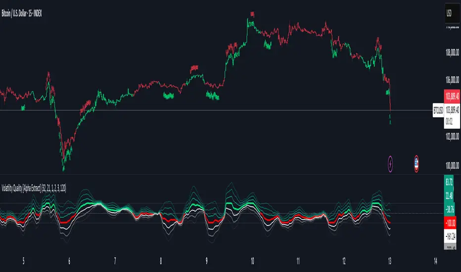
Volatility Quality [Alpha Extract]The Alpha-Extract Volatility Quality (AVQ) Indicator provides traders with deep insights into market volatility by measuring the directional strength of price movements. This sophisticated momentum-based tool helps identify overbought and oversold conditions, offering actionable buy and sell signals based on volatility trends and standard deviation bands.
🔶 CALCULATION
The indicator processes volatility quality data through a series of analytical steps:
Bar Range Calculation: Measures true range (TR) to capture price volatility.
Directional Weighting: Applies directional bias (positive for bullish candles, negative for bearish) to the true range.
VQI Computation: Uses an exponential moving average (EMA) of weighted volatility to derive the Volatility Quality Index (VQI).
vqiRaw = ta.ema(weightedVol, vqiLen)
Smoothing: Applies an additional EMA to smooth the VQI for clearer signals.
Normalization: Optionally normalizes VQI to a -100/+100 scale based on historical highs and lows.
Standard Deviation Bands: Calculates three upper and lower bands using standard deviation multipliers for volatility thresholds.
vqiStdev = ta.stdev(vqiSmoothed, vqiLen)
upperBand1 = vqiSmoothed + (vqiStdev * stdevMultiplier1)
upperBand2 = vqiSmoothed + (vqiStdev * stdevMultiplier2)
upperBand3 = vqiSmoothed + (vqiStdev * stdevMultiplier3)
lowerBand1 = vqiSmoothed - (vqiStdev * stdevMultiplier1)
lowerBand2 = vqiSmoothed - (vqiStdev * stdevMultiplier2)
lowerBand3 = vqiSmoothed - (vqiStdev * stdevMultiplier3)
Signal Generation: Produces overbought/oversold signals when VQI reaches extreme levels (±200 in normalized mode).
Formula:
Bar Range = True Range (TR)
Weighted Volatility = Bar Range × (Close > Open ? 1 : Close < Open ? -1 : 0)
VQI Raw = EMA(Weighted Volatility, VQI Length)
VQI Smoothed = EMA(VQI Raw, Smoothing Length)
VQI Normalized = ((VQI Smoothed - Lowest VQI) / (Highest VQI - Lowest VQI) - 0.5) × 200
Upper Band N = VQI Smoothed + (StdDev(VQI Smoothed, VQI Length) × Multiplier N)
Lower Band N = VQI Smoothed - (StdDev(VQI Smoothed, VQI Length) × Multiplier N)
🔶 DETAILS
Visual Features:
VQI Plot: Displays VQI as a line or histogram (lime for positive, red for negative).
Standard Deviation Bands: Plots three upper and lower bands (teal for upper, grayscale for lower) to indicate volatility thresholds.
Reference Levels: Horizontal lines at 0 (neutral), +100, and -100 (in normalized mode) for context.
Zone Highlighting: Overbought (⋎ above bars) and oversold (⋏ below bars) signals for extreme VQI levels (±200 in normalized mode).
Candle Coloring: Optional candle overlay colored by VQI direction (lime for positive, red for negative).
Interpretation:
VQI ≥ 200 (Normalized): Overbought condition, strong sell signal.
VQI 100–200: High volatility, potential selling opportunity.
VQI 0–100: Neutral bullish momentum.
VQI 0 to -100: Neutral bearish momentum.
VQI -100 to -200: High volatility, strong bearish momentum.
VQI ≤ -200 (Normalized): Oversold condition, strong buy signal.
🔶 EXAMPLES
Overbought Signal Detection: When VQI exceeds 200 (normalized), the indicator flags potential market tops with a red ⋎ symbol.
Example: During strong uptrends, VQI reaching 200 has historically preceded corrections, allowing traders to secure profits.
Oversold Signal Detection: When VQI falls below -200 (normalized), a lime ⋏ symbol highlights potential buying opportunities.
Example: In bearish markets, VQI dropping below -200 has marked reversal points for profitable long entries.
Volatility Trend Tracking: The VQI plot and bands help traders visualize shifts in market momentum.
Example: A rising VQI crossing above zero with widening bands indicates strengthening bullish momentum, guiding traders to hold or enter long positions.
Dynamic Support/Resistance: Standard deviation bands act as dynamic volatility thresholds during price movements.
Example: Price reversals often occur near the third standard deviation bands, providing reliable entry/exit points during volatile periods.
🔶 SETTINGS
Customization Options:
VQI Length: Adjust the EMA period for VQI calculation (default: 14, range: 1–50).
Smoothing Length: Set the EMA period for smoothing (default: 5, range: 1–50).
Standard Deviation Multipliers: Customize multipliers for bands (defaults: 1.0, 2.0, 3.0).
Normalization: Toggle normalization to -100/+100 scale and adjust lookback period (default: 200, min: 50).
Display Style: Switch between line or histogram plot for VQI.
Candle Overlay: Enable/disable VQI-colored candles (lime for positive, red for negative).
The Alpha-Extract Volatility Quality Indicator empowers traders with a robust tool to navigate market volatility. By combining directional price range analysis with smoothed volatility metrics, it identifies overbought and oversold conditions, offering clear buy and sell signals. The customizable standard deviation bands and optional normalization provide precise context for market conditions, enabling traders to make informed decisions across various market cycles.
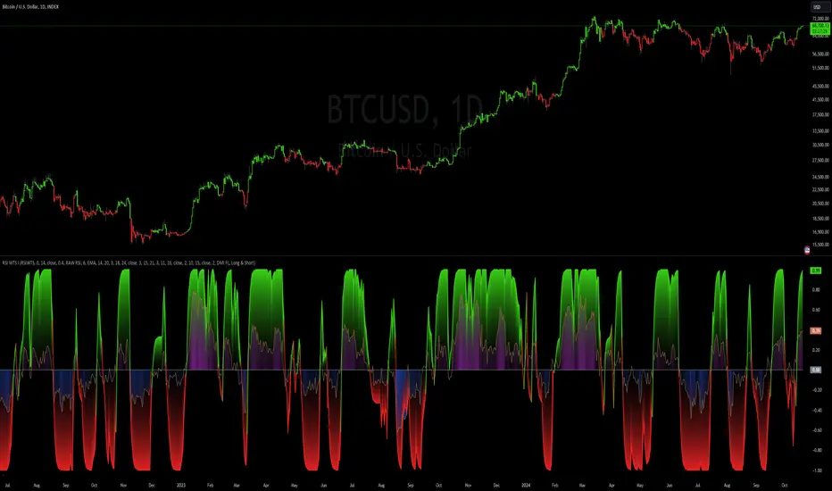
RSI Weighted Trend System I [InvestorUnknown]The RSI Weighted Trend System I is an experimental indicator designed to combine both slow-moving trend indicators for stable trend identification and fast-moving indicators to capture potential major turning points in the market. The novelty of this system lies in the dynamic weighting mechanism, where fast indicators receive weight based on the current Relative Strength Index (RSI) value, thus providing a flexible tool for traders seeking to adapt their strategies to varying market conditions.
Dynamic RSI-Based Weighting System
The core of the indicator is the dynamic weighting of fast indicators based on the value of the RSI. In essence, the higher the absolute value of the RSI (whether positive or negative), the higher the weight assigned to the fast indicators. This enables the system to capture rapid price movements around potential turning points.
Users can choose between a threshold-based or continuous weight system:
Threshold-Based Weighting: Fast indicators are activated only when the absolute RSI value exceeds a user-defined threshold. Below this threshold, fast indicators receive no weight.
Continuous Weighting: By setting the weight threshold to zero, the fast indicators always receive some weight, although this can result in more false signals in ranging markets.
// Calculate weight for Fast Indicators based on RSI (Slow Indicator weight is kept to 1 for simplicity)
f_RSI_Weight_System(series float rsi, simple float weight_thre) =>
float fast_weight = na
float slow_weight = na
if weight_thre > 0
if math.abs(rsi) <= weight_thre
fast_weight := 0
slow_weight := 1
else
fast_weight := 0 + math.sqrt(math.abs(rsi))
slow_weight := 1
else
fast_weight := 0 + math.sqrt(math.abs(rsi))
slow_weight := 1
Slow and Fast Indicators
Slow Indicators are designed to identify stable trends, remaining constant in weight. These include:
DMI (Directional Movement Index) For Loop
CCI (Commodity Channel Index) For Loop
Aroon For Loop
Fast Indicators are more responsive and designed to spot rapid trend shifts:
ZLEMA (Zero-Lag Exponential Moving Average) For Loop
IIRF (Infinite Impulse Response Filter) For Loop
Each of these indicators is calculated using a for-loop method to generate a moving average, which captures the trend of a given length range.
RSI Normalization
To facilitate the weighting system, the RSI is normalized from its usual 0-100 range to a -1 to 1 range. This allows for easy scaling when calculating weights and helps the system adjust to rapidly changing market conditions.
// Normalize RSI (1 to -1)
f_RSI(series float rsi_src, simple int rsi_len, simple string rsi_wb, simple string ma_type, simple int ma_len) =>
output = switch rsi_wb
"RAW RSI" => ta.rsi(rsi_src, rsi_len)
"RSI MA" => ma_type == "EMA" ? (ta.ema(ta.rsi(rsi_src, rsi_len), ma_len)) : (ta.sma(ta.rsi(rsi_src, rsi_len), ma_len))
Signal Calculation
The final trading signal is a weighted average of both the slow and fast indicators, depending on the calculated weights from the RSI. This ensures a balanced approach, where slow indicators maintain overall trend guidance, while fast indicators provide timely entries and exits.
// Calculate Signal (as weighted average)
sig = math.round(((DMI*slow_w) + (CCI*slow_w) + (Aroon*slow_w) + (ZLEMA*fast_w) + (IIRF*fast_w)) / (3*slow_w + 2*fast_w), 2)
Backtest Mode and Performance Metrics
This version of the RSI Weighted Trend System includes a comprehensive backtesting mode, allowing users to evaluate the performance of their selected settings against a Buy & Hold strategy. The backtesting includes:
Equity calculation based on the signals generated by the indicator.
Performance metrics table comparing Buy & Hold strategy metrics with the system’s signals, including: Mean, positive, and negative return percentages, Standard deviations (of all, positive and negative returns), Sharpe Ratio, Sortino Ratio, and Omega Ratio
f_PerformanceMetrics(series float base, int Lookback, simple float startDate, bool Annualize = true) =>
// Initialize variables for positive and negative returns
pos_sum = 0.0
neg_sum = 0.0
pos_count = 0
neg_count = 0
returns_sum = 0.0
returns_squared_sum = 0.0
pos_returns_squared_sum = 0.0
neg_returns_squared_sum = 0.0
// Loop through the past 'Lookback' bars to calculate sums and counts
if (time >= startDate)
for i = 0 to Lookback - 1
r = (base - base ) / base
returns_sum += r
returns_squared_sum += r * r
if r > 0
pos_sum += r
pos_count += 1
pos_returns_squared_sum += r * r
if r < 0
neg_sum += r
neg_count += 1
neg_returns_squared_sum += r * r
float export_array = array.new_float(12)
// Calculate means
mean_all = math.round((returns_sum / Lookback) * 100, 2)
mean_pos = math.round((pos_count != 0 ? pos_sum / pos_count : na) * 100, 2)
mean_neg = math.round((neg_count != 0 ? neg_sum / neg_count : na) * 100, 2)
// Calculate standard deviations
stddev_all = math.round((math.sqrt((returns_squared_sum - (returns_sum * returns_sum) / Lookback) / Lookback)) * 100, 2)
stddev_pos = math.round((pos_count != 0 ? math.sqrt((pos_returns_squared_sum - (pos_sum * pos_sum) / pos_count) / pos_count) : na) * 100, 2)
stddev_neg = math.round((neg_count != 0 ? math.sqrt((neg_returns_squared_sum - (neg_sum * neg_sum) / neg_count) / neg_count) : na) * 100, 2)
// Calculate probabilities
prob_pos = math.round((pos_count / Lookback) * 100, 2)
prob_neg = math.round((neg_count / Lookback) * 100, 2)
prob_neu = math.round(((Lookback - pos_count - neg_count) / Lookback) * 100, 2)
// Calculate ratios
sharpe_ratio = math.round(mean_all / stddev_all * (Annualize ? math.sqrt(Lookback) : 1), 2)
sortino_ratio = math.round(mean_all / stddev_neg * (Annualize ? math.sqrt(Lookback) : 1), 2)
omega_ratio = math.round(pos_sum / math.abs(neg_sum), 2)
// Set values in the array
array.set(export_array, 0, mean_all), array.set(export_array, 1, mean_pos), array.set(export_array, 2, mean_neg),
array.set(export_array, 3, stddev_all), array.set(export_array, 4, stddev_pos), array.set(export_array, 5, stddev_neg),
array.set(export_array, 6, prob_pos), array.set(export_array, 7, prob_neu), array.set(export_array, 8, prob_neg),
array.set(export_array, 9, sharpe_ratio), array.set(export_array, 10, sortino_ratio), array.set(export_array, 11, omega_ratio)
// Export the array
export_array
The metrics help traders assess the effectiveness of their strategy over time and can be used to optimize their settings.
Calibration Mode
A calibration mode is included to assist users in tuning the indicator to their specific needs. In this mode, traders can focus on a specific indicator (e.g., DMI, CCI, Aroon, ZLEMA, IIRF, or RSI) and fine-tune it without interference from other signals.
The calibration plot visualizes the chosen indicator's performance against a zero line, making it easy to see how changes in the indicator’s settings affect its trend detection.
Customization and Default Settings
Important Note: The default settings provided are not optimized for any particular market or asset. They serve as a starting point for experimentation. Traders are encouraged to calibrate the system to suit their own trading strategies and preferences.
The indicator allows deep customization, from selecting which indicators to use, adjusting the lengths of each indicator, smoothing parameters, and the RSI weight system.
Alerts
Traders can set alerts for both long and short signals when the indicator flips, allowing for automated monitoring of potential trading opportunities.
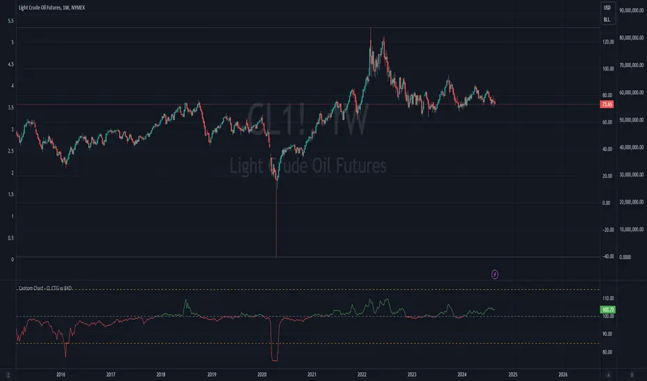
Cantom Chart - CL CTG vs BKDEnglish : This Pine Script indicator, named "Cantom Chart - CL CTG vs BKD," uniquely analyzes the immediate state of oil futures contracts to determine if they are in contango or backwardation. The script uses the price ratio between the nearest (CL1) and the next nearest (CL2) NYMEX crude oil futures contracts. It multiplies this ratio by 100 for clarity and scales fluctuations for enhanced visibility.
Key Features:
Dynamic Ratio Calculation: Computes the ratio (CL1/CL2 * 100) to determine the immediate market state.
Market State Interpretation: A ratio above 100 indicates backwardation, suggesting higher demand than supply, while a ratio below 100 indicates contango, suggesting higher supply than demand.
Volatility Adjustment: Amplifies market state changes by tripling the deviation from the baseline of 100, making it easier to observe subtle shifts.
Anomaly Detection: Caps the adjusted ratio at 125 for highs and 75 for lows, maintaining these limits until the ratio returns to normal levels.
Usage: This indicator is especially useful for traders analyzing supply-demand dynamics and inflationary pressures in the oil market. To apply it, simply add the script to your TradingView chart and adjust the 'Lower Threshold' and 'Upper Threshold' lines as needed based on your trading strategy.
-----
日本語 : この「Cantom Chart - CL CTG vs BKD」Pine Scriptインジケーターは、直近の原油先物契約がコンタンゴまたはバックワーデーションにあるかを特定するための独自の分析を提供します。最近の(CL1)と次の(CL2)NYMEX原油先物契約間の価格比を使用し、この比率に100を掛けて明確性を高め、変動の視認性を向上させます。
主要機能:
動的比率計算: 市場の即時状態を判断するために比率(CL1/CL2 * 100)を計算します。
市場状態の解釈: 比率が100を超える場合はバックワーデーション(需要が供給を上回る)、100未満の場合はコンタンゴ(供給が需要を上回る)を示します。
変動調整: 基準値100からの偏差を3倍にして、微妙な変化を容易に観察できるようにします。
異常値検出: 調整された比率を高値で125、低値で75に制限し、通常のレベルに戻るまでこれらの限界を維持します。
使用方法: このインジケーターは、原油市場における需給ダイナミクスとインフレ圧力を分析するトレーダーにとって特に有用です。使用するには、このスクリプトをTradingViewチャートに追加し、トレーディング戦略に基づいて「Lower Threshold」と「Upper Threshold」のラインを必要に応じて調整します。
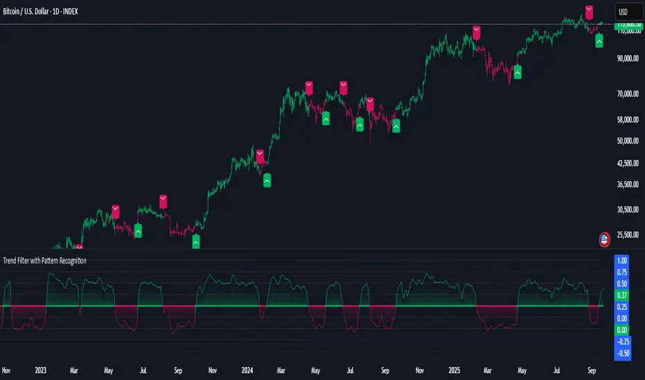
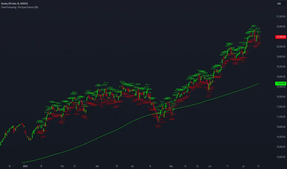
Trend Forecasting - The Quant Science🌏 Trend Forecasting | ENG 🌏
This plug-in acts as a statistical filter, adding new information to your chart that will allow you to quickly verify the direction of a trend and the probability with which the price will be above or below the average in the future, helping you to uncover probable market inefficiencies.
🧠 Model calculation
The model calculates the arithmetic mean in relation to positive and negative events within the available sample for the selected time series. Where a positive event is defined as a closing price greater than the average, and a negative event as a closing price less than the average. Once all events have been calculated, the probabilities are extrapolated by relating each event.
Example
Positive event A: 70
Negative event B: 30
Total events: 100
Probabilities A: (100 / 70) x 100 = 70%
Probabilities B: (100 / 30) x 100 = 30%
Event A has a 70% probability of occurring compared to Event B which has a 30% probability.
🔍 Information Filter
The data on the graph show the future probabilities of prices being above average (default in green) and the probabilities of prices being below average (default in red).
The information that can be quickly retrieved from this indicator is:
1. Trend: Above-average prices together with a constant of data in green greater than 50% + 1 indicate that the observed historical series shows a bullish trend. The probability is correlated proportionally to the value of the data; the higher and increasing the expected value, the greater the observed bullish trend. On the other hand, a below-average price together with a red-coloured data constant show quantitative data regarding the presence of a bearish trend.
2. Future Probability: By analysing the data, it is possible to find the probability with which the price will be above or below the average in the future. In green are classified the probabilities that the price will be higher than the average, in red are classified the probabilities that the price will be lower than the average.
🔫 Operational Filter .
The indicator can be used operationally in the search for investment or trading opportunities given its ability to identify an inefficiency within the observed data sample.
⬆ Bullish forecast
For bullish trades, the inefficiency will appear as a historical series with a bullish trend, with high probability of a bullish trend in the future that is currently below the average.
⬇ Bearish forecast
For short trades, the inefficiency will appear as a historical series with a bearish trend, with a high probability of a bearish trend in the future that is currently above the average.
📚 Settings
Input: via the Input user interface, it is possible to adjust the periods (1 to 500) with which the average is to be calculated. By default the periods are set to 200, which means that the average is calculated by taking the last 200 periods.
Style: via the Style user interface it is possible to adjust the colour and switch a specific output on or off.
🇮🇹Previsione Della Tendenza Futura | ITA 🇮🇹
Questo plug-in funge da filtro statistico, aggiungendo nuove informazioni al tuo grafico che ti permetteranno di verificare rapidamente tendenza di un trend, probabilità con la quale il prezzo si troverà sopra o sotto la media in futuro aiutandoti a scovare probabili inefficienze di mercato.
🧠 Calcolo del modello
Il modello calcola la media aritmetica in relazione con gli eventi positivi e negativi all'intero del campione disponibile per la serie storica selezionata. Dove per evento positivo si intende un prezzo alla chiusura maggiore della media, mentre per evento negativo si intende un prezzo alla chiusura minore della media. Calcolata la totalità degli eventi le probabilità vengono estrapolate rapportando ciascun evento.
Esempio
Evento positivo A: 70
Evento negativo B: 30
Totale eventi : 100
Formula A: (100 / 70) x 100 = 70%
Formula B: (100 / 30) x 100 = 30%
Evento A ha una probabilità del 70% di realizzarsi rispetto all' Evento B che ha una probabilità pari al 30%.
🔍 Filtro informativo
I dati sul grafico mostrano le probabilità future che i prezzi siano sopra la media (di default in verde) e le probabilità che i prezzi siano sotto la media (di default in rosso).
Le informazioni che si possono rapidamente reperire da questo indicatore sono:
1. Trend: I prezzi sopra la media insieme ad una costante di dati in verde maggiori al 50% + 1 indicano che la serie storica osservata presenta un trend rialzista. La probabilità è correlata proporzionalmente al valore del dato; tanto più sarà alto e crescente il valore atteso e maggiore sarà la tendenza rialzista osservata. Viceversa, un prezzo sotto la media insieme ad una costante di dati classificati in colore rosso mostrano dati quantitativi riguardo la presenza di una tendenza ribassista.
2. Probabilità future: analizzando i dati è possibile reperire la probabilità con cui il prezzo si troverà sopra o sotto la media in futuro. In verde vengono classificate le probabilità che il prezzo sarà maggiore alla media, in rosso vengono classificate le probabilità che il prezzo sarà minore della media.
🔫 Filtro operativo
L' indicatore può essere utilizzato a livello operativo nella ricerca di opportunità di investimento o di trading vista la capacità di identificare un inefficienza all'interno del campione di dati osservato.
⬆ Previsione rialzista
Per operatività di tipo rialzista l'inefficienza apparirà come una serie storica a tendenza rialzista, con alte probabilità di tendenza rialzista in futuro che attualmente si trova al di sotto della media.
⬇ Previsione ribassista
Per operatività di tipo short l'inefficienza apparirà come una serie storica a tendenza ribassista, con alte probabilità di tendenza ribassista in futuro che si trova attualmente sopra la media.
📚 Impostazioni
Input: tramite l'interfaccia utente Input è possibile regolare i periodi (da 1 a 500) con cui calcolare la media. Di default i periodi sono impostati sul valore di 200, questo significa che la media viene calcolata prendendo gli ultimi 200 periodi.
Style: tramite l'interfaccia utente Style è possibile regolare il colore e attivare o disattivare un specifico output.
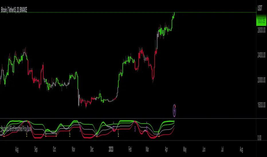
Stochastic RSI of Smoothed Price [Loxx]What is Stochastic RSI of Smoothed Price?
This indicator is just as it's title suggests. There are six different signal types, various price smoothing types, and seven types of RSI.
This indicator contains 7 different types of RSI:
RSX
Regular
Slow
Rapid
Harris
Cuttler
Ehlers Smoothed
What is RSI?
RSI stands for Relative Strength Index . It is a technical indicator used to measure the strength or weakness of a financial instrument's price action.
The RSI is calculated based on the price movement of an asset over a specified period of time, typically 14 days, and is expressed on a scale of 0 to 100. The RSI is considered overbought when it is above 70 and oversold when it is below 30.
Traders and investors use the RSI to identify potential buy and sell signals. When the RSI indicates that an asset is oversold, it may be considered a buying opportunity, while an overbought RSI may signal that it is time to sell or take profits.
It's important to note that the RSI should not be used in isolation and should be used in conjunction with other technical and fundamental analysis tools to make informed trading decisions.
What is RSX?
Jurik RSX is a technical analysis indicator that is a variation of the Relative Strength Index Smoothed ( RSX ) indicator. It was developed by Mark Jurik and is designed to help traders identify trends and momentum in the market.
The Jurik RSX uses a combination of the RSX indicator and an adaptive moving average (AMA) to smooth out the price data and reduce the number of false signals. The adaptive moving average is designed to adjust the smoothing period based on the current market conditions, which makes the indicator more responsive to changes in price.
The Jurik RSX can be used to identify potential trend reversals and momentum shifts in the market. It oscillates between 0 and 100, with values above 50 indicating a bullish trend and values below 50 indicating a bearish trend . Traders can use these levels to make trading decisions, such as buying when the indicator crosses above 50 and selling when it crosses below 50.
The Jurik RSX is a more advanced version of the RSX indicator, and while it can be useful in identifying potential trade opportunities, it should not be used in isolation. It is best used in conjunction with other technical and fundamental analysis tools to make informed trading decisions.
What is Slow RSI?
Slow RSI is a variation of the traditional Relative Strength Index ( RSI ) indicator. It is a more smoothed version of the RSI and is designed to filter out some of the noise and short-term price fluctuations that can occur with the standard RSI .
The Slow RSI uses a longer period of time than the traditional RSI , typically 21 periods instead of 14. This longer period helps to smooth out the price data and makes the indicator less reactive to short-term price fluctuations.
Like the traditional RSI , the Slow RSI is used to identify potential overbought and oversold conditions in the market. It oscillates between 0 and 100, with values above 70 indicating overbought conditions and values below 30 indicating oversold conditions. Traders often use these levels as potential buy and sell signals.
The Slow RSI is a more conservative version of the RSI and can be useful in identifying longer-term trends in the market. However, it can also be slower to respond to changes in price, which may result in missed trading opportunities. Traders may choose to use a combination of both the Slow RSI and the traditional RSI to make informed trading decisions.
What is Rapid RSI?
Same as regular RSI but with a faster calculation method
What is Harris RSI?
Harris RSI is a technical analysis indicator that is a variation of the Relative Strength Index ( RSI ). It was developed by Larry Harris and is designed to help traders identify potential trend changes and momentum shifts in the market.
The Harris RSI uses a different calculation formula compared to the traditional RSI . It takes into account both the opening and closing prices of a financial instrument, as well as the high and low prices. The Harris RSI is also normalized to a range of 0 to 100, with values above 50 indicating a bullish trend and values below 50 indicating a bearish trend .
Like the traditional RSI , the Harris RSI is used to identify potential overbought and oversold conditions in the market. It oscillates between 0 and 100, with values above 70 indicating overbought conditions and values below 30 indicating oversold conditions. Traders often use these levels as potential buy and sell signals.
The Harris RSI is a more advanced version of the RSI and can be useful in identifying longer-term trends in the market. However, it can also generate more false signals than the standard RSI . Traders may choose to use a combination of both the Harris RSI and the traditional RSI to make informed trading decisions.
What is Cuttler RSI?
Cuttler RSI is a technical analysis indicator that is a variation of the Relative Strength Index ( RSI ). It was developed by Curt Cuttler and is designed to help traders identify potential trend changes and momentum shifts in the market.
The Cuttler RSI uses a different calculation formula compared to the traditional RSI . It takes into account the difference between the closing price of a financial instrument and the average of the high and low prices over a specified period of time. This difference is then normalized to a range of 0 to 100, with values above 50 indicating a bullish trend and values below 50 indicating a bearish trend .
Like the traditional RSI , the Cuttler RSI is used to identify potential overbought and oversold conditions in the market. It oscillates between 0 and 100, with values above 70 indicating overbought conditions and values below 30 indicating oversold conditions. Traders often use these levels as potential buy and sell signals.
The Cuttler RSI is a more advanced version of the RSI and can be useful in identifying longer-term trends in the market. However, it can also generate more false signals than the standard RSI . Traders may choose to use a combination of both the Cuttler RSI and the traditional RSI to make informed trading decisions.
What is Ehlers Smoothed RSI?
Ehlers smoothed RSI is a technical analysis indicator that is a variation of the Relative Strength Index ( RSI ). It was developed by John Ehlers and is designed to help traders identify potential trend changes and momentum shifts in the market.
The Ehlers smoothed RSI uses a different calculation formula compared to the traditional RSI . It uses a smoothing algorithm that is designed to reduce the noise and random fluctuations that can occur with the standard RSI . The smoothing algorithm is based on a concept called "digital signal processing" and is intended to improve the accuracy of the indicator.
Like the traditional RSI , the Ehlers smoothed RSI is used to identify potential overbought and oversold conditions in the market. It oscillates between 0 and 100, with values above 70 indicating overbought conditions and values below 30 indicating oversold conditions. Traders often use these levels as potential buy and sell signals.
The Ehlers smoothed RSI can be useful in identifying longer-term trends and momentum shifts in the market. However, it can also generate more false signals than the standard RSI . Traders may choose to use a combination of both the Ehlers smoothed RSI and the traditional RSI to make informed trading decisions.
What is Stochastic RSI?
Stochastic RSI (StochRSI) is a technical analysis indicator that combines the concepts of the Stochastic Oscillator and the Relative Strength Index (RSI). It is used to identify potential overbought and oversold conditions in financial markets, as well as to generate buy and sell signals based on the momentum of price movements.
To understand Stochastic RSI, let's first define the two individual indicators it is based on:
Stochastic Oscillator: A momentum indicator that compares a particular closing price of a security to a range of its prices over a certain period. It is used to identify potential trend reversals and generate buy and sell signals.
Relative Strength Index (RSI): A momentum oscillator that measures the speed and change of price movements. It ranges between 0 and 100 and is used to identify overbought or oversold conditions in the market.
Now, let's dive into the Stochastic RSI:
The Stochastic RSI applies the Stochastic Oscillator formula to the RSI values, essentially creating an indicator of an indicator. It helps to identify when the RSI is in overbought or oversold territory with more sensitivity, providing more frequent signals than the standalone RSI.
The formula for StochRSI is as follows:
StochRSI = (RSI - Lowest Low RSI) / (Highest High RSI - Lowest Low RSI)
Where:
RSI is the current RSI value.
Lowest Low RSI is the lowest RSI value over a specified period (e.g., 14 days).
Highest High RSI is the highest RSI value over the same specified period.
StochRSI ranges from 0 to 1, but it is usually multiplied by 100 for easier interpretation, making the range 0 to 100. Like the RSI, values close to 0 indicate oversold conditions, while values close to 100 indicate overbought conditions. However, since the StochRSI is more sensitive, traders typically use 20 as the oversold threshold and 80 as the overbought threshold.
Traders use the StochRSI to generate buy and sell signals by looking for crossovers with a signal line (a moving average of the StochRSI), similar to the way the Stochastic Oscillator is used. When the StochRSI crosses above the signal line, it is considered a bullish signal, and when it crosses below the signal line, it is considered a bearish signal.
It is essential to use the Stochastic RSI in conjunction with other technical analysis tools and indicators, as well as to consider the overall market context, to improve the accuracy and reliability of trading signals.
Signal types included are the following;
Fixed Levels
Floating Levels
Quantile Levels
Fixed Middle
Floating Middle
Quantile Middle
Extras
Alerts
Bar coloring
Loxx's Expanded Source Types
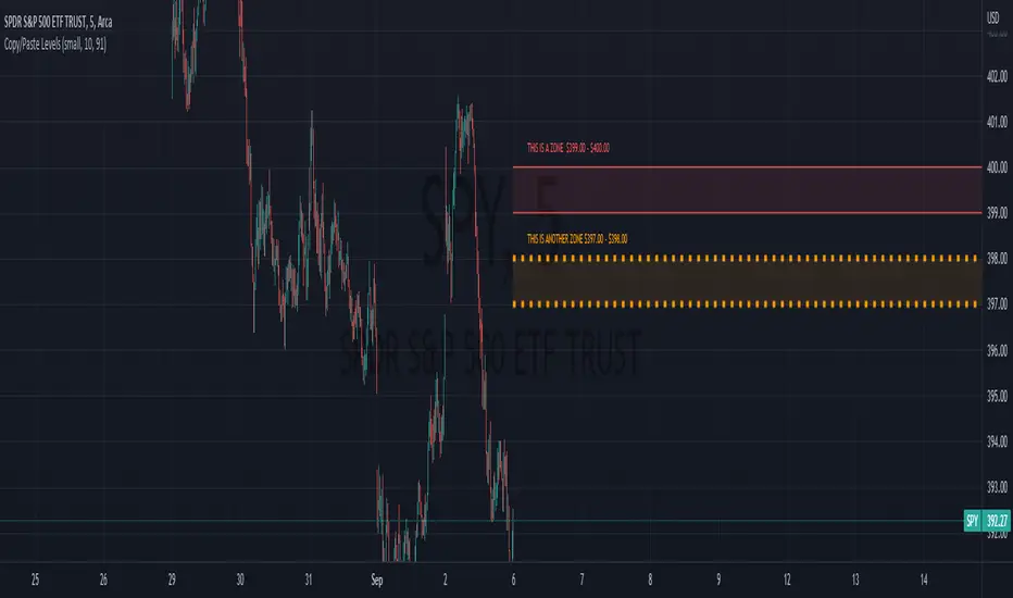
Copy/Paste LevelsCopy/Paste Levels allows levels to be pasted onto your chart from a properly formatted source.
This tool streamlines the process of adding lines to your chart, and sharing lines from your chart.
More than one ticker at a time!
This indicator will only draw lines on charts it has values for!
This means you can input levels for every ticker you need all at once, one time, and only be displayed the levels for the current chart you are looking at. When you switch tickers, the levels for that ticker will display. (Assuming you have levels entered for that ticker)
The formatting is as follows:
Ticker,Color,Style,Width,Lvl1,Lvl2,Lvl3;
Ticker - Any ticker on Tradingview can be used in the field
Color - Available colors are: Red,Orange,Yellow,Green,Blue,Purple,White,Black,Gray
Style - Available styles are: Solid,Dashed,Dotted
Width - This can be any negative integer, ex.(-1,-2,-3,-4,-5)
Lvls - These can be any positive number (decimals allowed)
Semi-Colons separate sections, each section contains enough information to create at least 1 line.
Each additional level added within the same section will have the same styling parameters as the other levels in the section.
Example:
2 solid lines colored red with a thickness of 2 on QQQ, 1 at $300 and 1 at $400.
QQQ,RED,SOLID,-2,300,400;
IMPORTANT MUST READ!!!
Remember to not include any spaces between commas and the entries in each field!
ex. ; QQQ, red, dotted, -1, 325; <- Wrong
ex. ;QQQ,red,dotted,-1,325;)<- Right
However,
All fields must be filled out, to use default values in the fields, insert a space between the commas.
ex. ;QQQ,red,dotted,,325; <- Wrong
ex. ;QQQ,red,dotted, ,325; <- Right
While spaces can not be included line breaks can!
I recommend for easier typing and viewing to include a line break for each new line (if changing styling or ticker)
Example:
2 solid lines, one red at $300, one green at $400, both default width. Written in a single line AND using multiple lines, both give the same output.
QQQ,red,solid, ,300;QQQ,green,solid, ,400;
or
QQQ,red,solid, ,300;
QQQ,green,solid, ,400;
In this following screenshot you can see more examples of different formatting variations.
The textbox contains exactly what is pasted into the settings input box.
As you can see, capitalization does not matter.
Default Values:
Color = optimal contrast color, If this field is filled in with a space it will display the optimal contrast color of the users background.
Style = solid
Width = -1
More Examples:
Multi-Ticker: drawing 3 lines at $300, all default values, on 3 different tickers
SPY, , , ,300;QQQ, , , ,300;AAPL, , , ,300
or
SPY, , , ,300;
QQQ, , , ,300;
AAPL, , , ,300
Multiple levels: There is no limit* to the number of levels that can be included within 1 section.
* only TV default line limit per indicator (500)
This will be 4 lines all with the same styling at different values on 2 separate tickers.
SPY,BLUE,SOLID,-2,100,200,300,400;QQQ,BLUE,SOLID,-2,100,200,300,400
or
SPY,BLUE,SOLID,-2,100,200,300,400;
QQQ,BLUE,SOLID,-2,100,200,300,400
Semi-colons must separate sections, but are not required at the beginning or end, it makes no difference if they are or are not added.
SPY,BLUE,SOLID,-2,100,200,300,400;
QQQ,BLUE,SOLID,-2,100,200,300,400
==
SPY,BLUE,SOLID,-2,100,200,300,400;
QQQ,BLUE,SOLID,-2,100,200,300,400;
==
;SPY,BLUE,SOLID,-2,100,200,300,400;
QQQ,BLUE,SOLID,-2,100,200,300,400;
All the above output the same results.
Hope this is helpful for people,
Enjoy!
Stochastic RSI - WT Confluence Signal Detectors (TraderDemircan)Description
What This Indicator Does:
This indicator combines two powerful momentum oscillators—WaveTrend and Stochastic RSI—to identify high-probability trading signals through confluence. Instead of relying on a single indicator that may generate false signals, this tool only triggers buy/sell alerts when both oscillators simultaneously confirm extreme market conditions and trend reversals. This confluence approach significantly reduces noise and helps traders focus on the most reliable setups.
Key Features:
Dual-Oscillator Confluence: Generates signals only when both WaveTrend crossovers and Stochastic RSI extreme levels align
Normalized Scale Display: Both oscillators are plotted on a unified -100 to +100 scale for easy visual comparison
Visual Signal Confirmation: Clear intersection points marked with colored circles, plus optional candle coloring at crossover moments
Customizable Thresholds: Adjust overbought/oversold levels for both oscillators to match your trading style and asset volatility
Clean Visual Presentation: Optional area fill showing WaveTrend momentum difference, making divergences easier to spot
How It Works:
The indicator operates on a confluence principle where multiple conditions must align:
For BUY Signals (Green):
WaveTrend 1 crosses above WaveTrend 2 (bullish crossover)
WaveTrend is in oversold territory (below -53 or -60)
Stochastic RSI K-line is below 20 (oversold)
For SELL Signals (Red):
WaveTrend 1 crosses below WaveTrend 2 (bearish crossover)
WaveTrend is in overbought territory (above 53 or 60)
Stochastic RSI K-line is above 80 (overbought)
WaveTrend Component:
Uses the hlc3 price (average of high, low, close) to calculate a channel index that identifies market momentum waves. The two WaveTrend lines (WT1 and WT2) act similarly to MACD, where crossovers indicate momentum shifts. The oscillator ranges from approximately -100 to +100, with extreme values suggesting potential reversals.
Stochastic RSI Component:
Applies stochastic calculations to RSI values rather than raw price, creating a more sensitive momentum indicator. Values above 80 indicate overbought conditions (potential selling opportunity), while values below 20 indicate oversold conditions (potential buying opportunity). The indicator includes both K-line (faster) and D-line (slower, smoothed) for additional confirmation.
Normalization Technology:
To enable direct visual comparison, the Stochastic RSI (normally 0-100 scale) is normalized to match WaveTrend's -100 to +100 scale. This allows traders to see both oscillators' movements in relation to the same reference levels, making divergences and convergences more apparent.
How to Use:
For Trend Traders:
Wait for confluence signals in the direction of the larger trend
Use buy signals in uptrends as entry points during pullbacks
Use sell signals in downtrends as entry points during bounces
For Reversal Traders:
Focus on confluence signals at major support/resistance levels
Look for divergences between price and oscillators before confluence signals
Consider stronger signals when both oscillators reach extreme levels (WT beyond ±60, Stoch beyond 20/80)
For Scalpers:
Lower the WaveTrend Channel Length (default 10) to 5-7 for more frequent signals
Tighten overbought/oversold thresholds slightly (e.g., WT: ±50, Stoch: 30/70)
Use on lower timeframes (5m, 15m) with strict stop losses
Settings Guide:
WaveTrend Parameters:
Channel Length (10): Controls sensitivity. Lower = more signals but more noise. Higher = fewer but more reliable signals
Average Length (21): Smoothing period for WT2. Higher values reduce whipsaws
Overbought Levels (60/53): Two-tier system. Breaching 60 indicates strong overbought, 53 is moderate
Oversold Levels (-60/-53): Mirror of overbought levels for downside extremes
Stochastic RSI Parameters:
K-Smooth (3): Smoothing for the K-line. Higher = smoother but delayed
D-Smooth (3): Additional smoothing for the D-line signal
RSI Period (14): Standard RSI calculation period
Stoch Period (14): Stochastic calculation lookback
Oversold (20) / Overbought (80): Classic thresholds for extreme conditions
Visual Options:
Show WT Difference Area: Displays the momentum difference between WT1 and WT2 as a blue shaded area
Show WT Intersection Points: Marks crossover points with colored circles (red for bearish, green for bullish)
Color Candles at Intersection: Changes candle colors at crossover moments (blue for bearish, yellow for bullish)
Show Stoch Over Signals: Displays when Stochastic RSI breaches extreme levels
What Makes This Original:
While WaveTrend and Stochastic RSI are established indicators, this script's originality lies in:
Confluence Logic: The specific combination requiring simultaneous confirmation from both oscillators in extreme zones, not just simple crossovers
Normalization Approach: Displaying both oscillators on the same -100 to +100 scale for direct visual comparison, which is not standard
Multi-Tier Overbought/Oversold: Using two levels (60/53) instead of one, allowing for nuanced signal strength assessment
Integrated Visual System: Combining area fills, intersection markers, and candle coloring in a coordinated display that shows momentum flow at a glance
Important Considerations:
This is a momentum-based oscillator system, which performs best in ranging or trending markets with clear swings
In strong trending markets, the oscillator may remain in extreme zones for extended periods (remain overbought during strong uptrends, oversold during strong downtrends)
Confluence signals are intentionally rare to maintain quality—expect fewer signals than with single-indicator systems
Always combine with price action analysis, support/resistance levels, and proper risk management
Not recommended for extremely low volatility or thin markets where oscillators may produce erratic readings
Best Timeframes:
Intraday: 15m, 1H (with tighter parameters)
Swing Trading: 4H, Daily (with default parameters)
Position Trading: Daily, Weekly (with extended Channel Length 15-20)
Typical Use Cases:
Identifying exhaustion points in trending markets
Timing entries during pullbacks in established trends
Spotting potential reversal zones at key price levels
Filtering out weak momentum signals during consolidation

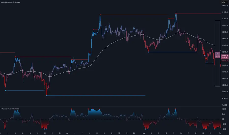
MA Oscillator Map [ChartPrime]⯁ OVERVIEW
The MA Oscillator Map transforms moving average deviations into an oscillator framework that highlights overextended price conditions. By normalizing the difference between price and a chosen moving average, the tool maps oscillations between -100 and +100 , with gradient coloring to emphasize bullish and bearish momentum. When the oscillator cools from extreme levels (-100/100), the indicator marks potential reversal points and extends short-term levels from those extremes. A compact side table and dynamic bar coloring make momentum context visible at a glance.
⯁ KEY FEATURES
Oscillator Mapping (±100 Scale):
Price deviation from the selected MA is normalized into a percentage scale, allowing consistent overbought/oversold readings across assets and timeframes.
// MA
MA = ma(close, maLengthInput, maTypeInput)
diff = src - MA
maxVal = ta.highest(math.abs(diff), 50)
osc = diff / maxVal * 100
Customizable MA Types:
Choose SMA, EMA, SMMA, WMA, or VWMA to fine-tune the smoothing method that powers the oscillator.
Extreme Signal Diamonds:
When the oscillator retreats from +100 or -100, the script plots diamonds to flag potential exhaustion and reversal zones.
Dynamic Levels from Extremes:
Upper and lower dotted lines extend from recent overextension points, projecting temporary barriers until broken by price.
Gradient Bar Coloring:
Candles and oscillator values adopt a bullish-to-bearish gradient, making shifts in momentum instantly visible on the chart.
Compact Momentum Map:
A table at the chart’s edge plots the oscillator position with a gradient scale and live percentage label for precise momentum tracking.
⯁ USAGE
Watch for diamonds after the oscillator exits ±100 — these mark potential exhaustion zones.
Use extended dotted levels as short-term reference lines; if broken, trend continuation is favored.
Combine gradient bar coloring with oscillator shifts for confirmation of momentum reversals.
Experiment with different MA types to adapt sensitivity for trending vs. ranging markets.
Use the side momentum table as a quick-read gauge of trend strength in percent terms.
⯁ CONCLUSION
The MA Oscillator Map reframes moving average deviations into a visual momentum tracker with extremes, reversal signals, and dynamic levels. By blending oscillator math with intuitive visuals like gradient candles, diamonds, and a live gauge, it helps traders spot overextension, exhaustion, and momentum shifts across any market.
Free Stock ScreenerMissing great trade opportunities is annoying, and unless you have 12 screens or only trade one market, you are missing a lot of trades. To fix that, we created this free stock screener so you get notified instantly of potential great trading conditions in real time, right on your chart.
You get notified of trading benchmarks being met by the value being displayed on the scanner as well as a color change so that it grabs your attention and makes you aware that you should take a look at the other market and look for a potential trade. It also has built in alerts so you can have an alert notification go off when any of your trading conditions are met instead of needing to watch the scanner for color changes.
The screener will change the ticker symbol background color to red green when price is above or below the previous daily range and above or below both VWAPs. This signals that the ticker is trending, which typically means it is a great time to trade that market and follow the trend.
This free stock screener allows you to scan up to 10 different markets at the same time for various different conditions so you always know what is going on with your favorite trading symbols. If you want to scan more tickers, just add the indicator to your chart again and change the table position to the other side of the screen and update the tickers on the 2nd screener, allowing you to have 20 tickers at a time.
The scanner can be fully customized by changing the markets that it screens and turning on or off as many of them as you would like. You can also turn on or off any of the different data sets so that you only get information about trading conditions that matter to you.
The screener can provide data on any type of market, such as stocks, crypto, futures, forex and more. Each ticker can be adjusted to whatever market you would like it to scan for data in the settings panel, the only limitation is that it will not provide data for the VWAP and volume trend score if the ticker you are screening does not provide volume data.
Screener Features
The scanner will provide the following types of data for each ticker that is turned on:
Volume - Provides a volume score compared to the average volume and notifies you of higher than normal volume and volume spikes on individual bars by changing colors.
Volatility - Provides a volatility score compared to the average volatility and notifies you of higher than normal volatility by changing colors.
Oscillator - Choose between the RSI or CCI. The value of that oscillator will be displayed and will notify you when values are in extreme ranges such as overbought or oversold conditions according to the threshold values you enter in the settings panel. When those thresholds have been breached, you will be notified by it changing color.
Big Candles - Compares the current candle to average previous candle sizes, and changes color to notify you of big candles including a big top wick, big bottom wick, big candle body and big candle high to low range.
Daily Level Touches & Trends - Calculates and displays various daily candle and intraday open price levels that act as support and resistance. Notifies you when price is touching any of the daily levels that are turned on. The levels you can have on are as follows: previous day high, previous day low or previous day open. It also will notify you when price is touching the current day’s open, NY 930am open, Asia 8pm open, London 2am open and NY midnight 12am open. It will also say “Above” if price is above the previous day’s high or it will say “Below” if price is below the previous day’s low. The color of the cell will also change when a level touch is happening or price is above the previous day high or below the previous day low.
VWAP - Choose from 2 different VWAP lengths, default settings are daily and weekly VWAPs. You will get notified if price touches either of the VWAPs and they will also say “Above” or “Below” if price is currently above or below each VWAP.
How To Use The Screener To Help You Trade
The main purpose of the screener is to scan other markets and notify you of potential good trading opportunities such as price bouncing off of the daily levels or VWAPs. It can also be used to know when price is trending according to the VWAPs and daily levels. Lastly, you can use it to know how the volume and volatility trends are currently which gives you more confidence in taking a trade with this data when volume and volatility are present.
Volume Score
When volume is high, this represents a good time to trade because there are many market participants and price is likely to be volatile while there is high volume which can present a lot of good trade setups for you to take.
The volume score shown on the screener measures the current volume trend compared to previous volume trends and calculates that into a score based on 100 being the same as the previous volume trend. So any value above 100 means it is high volume and any value less than 100 means it is lower volume than normal.
In the settings panel, you can adjust the volume threshold that needs to be met for a volume notification to show up. The default setting is at 120, so you will get notified when the current volume trend score is 120 or higher or you can adjust that threshold value to whatever value you prefer.
It also will notify you when there is a volume spike on the current bar. This is determined by calculating an average of the recent volume totals and then checking to see if the current bar is greater than or equal to that average multiplied by 3. So if a single bar has volume that is greater than 3 times what the average volume is, then you will get a notification that says “Spike” to make you aware of that volume spike.
The volume trend threshold, volume spike multiplier and lookback length for the average volume used in volume spike calculations can all be adjusted in the settings panel to fit your desired preferences.
Volatility Score
High volatility can mean it is a great time to trade because the market is moving quickly and providing large enough movements that you can get in and out in a short amount of time, while still accruing decent sized trade PnL.
The volatility score will calculate the current volatility for each market compared to previous conditions and then divide the current volatility by the average volatility to give you a volatility score. Anything over 100 means the market is decently volatile and you should look at that market to find potential trade setups to execute on. Anything below 100 means the market is not very volatile and it is usually best to just wait until volatility returns before you start trading again.
The screener will notify you when the volatility score is above the threshold you set. The default value is set to 90, but can be adjusted to your preference. Pay attention to any market that shows an alert and take a look at that chart because the high volatility may present a good trade setup for you in the near future.
Oscillator Score
The oscillator data can be switched between Relative Strength Index(RSI) and Commodity Channel Index(CCI).
The RSI provides a value between 0 and 100 that indicates the momentum and strength of the recent price action. Many traders use the extremes of the 0-100 range to signal overbought or oversold conditions and use that as a sign to look for price to reverse in the near future. The typical values used for this and the default settings to provide notifications are: 70 for overbought and 30 for oversold. The scanner will notify you when the RSI value is considered overbought or oversold so you know to take a look at the chart and analyze if it is ready for a trade to be taken.
The CCI provides a value that can be used to determine the trend strength of the underlying asset when the oscillator moves above 100 or below -100. These extreme values are outside of the normal accumulation range and signify that price is moving strongly in that direction so it may be a good time to take a trade in the direction of the trend. The scanner will show you the value of the CCI for each market and notify you if that value is above 100 or below -100.
Both RSI and CCI settings can be adjusted in the settings panel to your desired settings so you have the exact oscillator settings you prefer to use as well as the exact values that you want to use for being notified.
Big Candles
Big candles can mean that many traders are buying or selling at the same time and many times indicate a good signal to trade in that same direction. That is why we included this calculation in the screener, so you are always aware when a large candle prints.
It calculates the average size of the recent candles and then uses that average as the benchmark to determine if the current candle is considered big and worthy of notifying you to take a look at that chart.
You can adjust the multiplier used for the big candle threshold to whatever you desire, but the default setting is 3 which means the candle will be considered big and notify you if it is 3 times as large as an average candle.
The big candles data will track the following candle values and notify you with these labels:
High to Low candle size = HL
Candle Body from open to close candle size = OC
Top Wick size = TW
Bottom Wick size = BW
Daily Level Touches & Trend
Daily level touches are excellent levels to watch for price to bounce because they often act as support and resistance levels for intraday trading. The scanner will track each market and notify you when the current candle is touching any of the daily levels that you have turned on in the settings panel.
The main levels that are turned on by default and are useful for all markets and how they will be labeled on the scanner are as follows:
Previous Day High = High
Previous Day Low = Low
Previous Day Open = < Open
Previous Day Close = Close
Current Day Open = Open
We also included some extra levels that are useful for futures traders. They are as follows:
NY 930am Open = 930am
NY 12am Midnight Open = 12am
Asia Open at 8pm NY time = Asia
London Open at 2am NY Time = London
Watch how price reacts to these levels and then trade the bounces off of these levels if the price action confirms that it is going to respect that level.
When price is currently above the previous day high, the scanner will say “Above” and show a green color, indicating a bullish trend and that price is above the previous daily candle’s high.
When price is currently below the previous day low, the scanner will say “Below” and show a red color, indicating a bearish trend and that price is below the previous daily candle’s low.
Pay attention to when price is trending above or below the previous daily candle as those trends can provide excellent trend trading opportunities.
The daily levels that you have turned on in the settings will also show as lines on the chart and include a label next to them, identifying each level so you know what each line represents. You can turn on or off all of the lines shown on the chart in the main settings or turn them off one by one in the style panel of the settings. Labels can also be turned on or off for all of the lines in the main settings panel. You can adjust the label positioning in the Label Offset section of the settings panel.
VWAP Touches & Trend
VWAP stands for volume weighted average price and is a very popular tool that traders use to determine trend direction based on volume as well as an excellent level to trade price bounces off of.
The typical VWAP time period used is Daily, which means the volume weighted average price will reset at the beginning of a new day. We set the first VWAP to be the daily VWAP by default and the second one to be the weekly VWAP. You can adjust both of the time periods to be any of the provided time lengths that you choose.
The screener will show “Above” with a green background color when price is above the VWAP, indicating a bullish trend. It will show “Below” with a red background color when price is below the VWAP, indicating a bearish trend. When both VWAPs are showing Above or Below, you can expect price to trend in that direction, so look for pullbacks you can trade in the direction of the trend. If the VWAPs are showing different directions, then you should expect to bounce back and forth between the VWAPs, but be careful and watch out for price to break beyond either one and start a trend.
When the current candle is touching the VWAP, the scanner will change colors and say VWAP to notify you that price is touching the VWAP and you should look at that chart and analyze the market for a potential bounce off of the VWAP to trade.
Trending Market Signals
Strong trends are excellent markets to trade and can many times provide excellent trading opportunities that don’t require expert price action reading skills to be able to take winning trades from. That is why we included a signal to notify you of a strong trending market.
The strong trending market will show up as a green or red background color for the ticker name. If the color of the ticker name is green, it is notifying you that the price is above the previous daily high, above VWAP 1 and above VWAP 2 and is a good market to look for bullish trend trades. If the color of the ticker name is red, it is notifying you that the price is below the previous daily low, below VWAP 1 and below VWAP 2 and is a good market to look for bearish trend trades.
Changing The Tickers It Scans
To change the tickers that the indicator scans, scroll near the bottom of the settings panel and select the ticker symbol you want to update and then search for the exact symbol you want to use. If you want to scan less tickers, then just turn some of the tickers off that you don’t need.
Scanning More Than 10 Tickers
If you want to scan more than 10 tickers, you can add the scanner to your chart again and then just change the table position to the other side of the screen. This will allow you to scan 10 more tickers that will show up separately. Then if you want even more, just add the indicator to your chart again and update the table position until you have as many markets as you want. The table position setting can be found at the bottom of the main settings panel.
Alerts
The screener has alerts that can be used to notify you when any of the data set thresholds have been met or if price is touching one of the levels. You can set alerts for the following events:
Bullish Trend Alert - Price is above the previous daily high and above both VWAPs.
Bearish Trend Alert - Price is below the previous daily low and below both VWAPs.
High Volume Alert - Volume is higher than the threshold or a volume spike is detected.
High Volatility Alert - Volatility is higher than the threshold.
Oscillator Is Extended Alert - Oscillator value has exceeded the upper or lower threshold.
Big Candle Alert - A big candle has been detected.
Daily Level Touch Alert - One of the daily levels that is turned on is being touched.
VWAP Touch Alert - One of the 2 VWAPs are being touched.
An alert will trigger when any one of tickers on your scanner meets the alert conditions, so when you see the alert, you will need to go to your chart and look at the scanner to see which ticker it was and then navigate to that chart to look for potential trade setups.
The alerts will use the exact same settings you have configured in the settings panel to send you alert notifications. With normal settings, this could give you a lot of alerts, so if you only want alerts to fire when abnormal conditions are being met, try setting up a second screener on your chart that has very high threshold values and only has the most important level touches on. Then turn the setting "Do Not Show The Screener On The Chart" to off so the calculations will still run and fire alerts, but won't clog up your charts. This way you can only get alert notifications when major events happen but still have your normal screener settings available on your chart.
Markets This Can Be Used On
This screener uses the price action and volume data so you can use it to scan any type of market you would like as long as the ticker you are scanning has price and volume data feeds. If a market does not have volume data, then it will just show NaN in the volume row and the VWAP rows will not show anything.

Kelly Position Size CalculatorThis position sizing calculator implements the Kelly Criterion, developed by John L. Kelly Jr. at Bell Laboratories in 1956, to determine mathematically optimal position sizes for maximizing long-term wealth growth. Unlike arbitrary position sizing methods, this tool provides a scientifically solution based on your strategy's actual performance statistics and incorporates modern refinements from over six decades of academic research.
The Kelly Criterion addresses a fundamental question in capital allocation: "What fraction of capital should be allocated to each opportunity to maximize growth while avoiding ruin?" This question has profound implications for financial markets, where traders and investors constantly face decisions about optimal capital allocation (Van Tharp, 2007).
Theoretical Foundation
The Kelly Criterion for binary outcomes is expressed as f* = (bp - q) / b, where f* represents the optimal fraction of capital to allocate, b denotes the risk-reward ratio, p indicates the probability of success, and q represents the probability of loss (Kelly, 1956). This formula maximizes the expected logarithm of wealth, ensuring maximum long-term growth rate while avoiding the risk of ruin.
The mathematical elegance of Kelly's approach lies in its derivation from information theory. Kelly's original work was motivated by Claude Shannon's information theory (Shannon, 1948), recognizing that maximizing the logarithm of wealth is equivalent to maximizing the rate of information transmission. This connection between information theory and wealth accumulation provides a deep theoretical foundation for optimal position sizing.
The logarithmic utility function underlying the Kelly Criterion naturally embodies several desirable properties for capital management. It exhibits decreasing marginal utility, penalizes large losses more severely than it rewards equivalent gains, and focuses on geometric rather than arithmetic mean returns, which is appropriate for compounding scenarios (Thorp, 2006).
Scientific Implementation
This calculator extends beyond basic Kelly implementation by incorporating state of the art refinements from academic research:
Parameter Uncertainty Adjustment: Following Michaud (1989), the implementation applies Bayesian shrinkage to account for parameter estimation error inherent in small sample sizes. The adjustment formula f_adjusted = f_kelly × confidence_factor + f_conservative × (1 - confidence_factor) addresses the overconfidence bias documented by Baker and McHale (2012), where the confidence factor increases with sample size and the conservative estimate equals 0.25 (quarter Kelly).
Sample Size Confidence: The reliability of Kelly calculations depends critically on sample size. Research by Browne and Whitt (1996) provides theoretical guidance on minimum sample requirements, suggesting that at least 30 independent observations are necessary for meaningful parameter estimates, with 100 or more trades providing reliable estimates for most trading strategies.
Universal Asset Compatibility: The calculator employs intelligent asset detection using TradingView's built-in symbol information, automatically adapting calculations for different asset classes without manual configuration.
ASSET SPECIFIC IMPLEMENTATION
Equity Markets: For stocks and ETFs, position sizing follows the calculation Shares = floor(Kelly Fraction × Account Size / Share Price). This straightforward approach reflects whole share constraints while accommodating fractional share trading capabilities.
Foreign Exchange Markets: Forex markets require lot-based calculations following Lot Size = Kelly Fraction × Account Size / (100,000 × Base Currency Value). The calculator automatically handles major currency pairs with appropriate pip value calculations, following industry standards described by Archer (2010).
Futures Markets: Futures position sizing accounts for leverage and margin requirements through Contracts = floor(Kelly Fraction × Account Size / Margin Requirement). The calculator estimates margin requirements as a percentage of contract notional value, with specific adjustments for micro-futures contracts that have smaller sizes and reduced margin requirements (Kaufman, 2013).
Index and Commodity Markets: These markets combine characteristics of both equity and futures markets. The calculator automatically detects whether instruments are cash-settled or futures-based, applying appropriate sizing methodologies with correct point value calculations.
Risk Management Integration
The calculator integrates sophisticated risk assessment through two primary modes:
Stop Loss Integration: When fixed stop-loss levels are defined, risk calculation follows Risk per Trade = Position Size × Stop Loss Distance. This ensures that the Kelly fraction accounts for actual risk exposure rather than theoretical maximum loss, with stop-loss distance measured in appropriate units for each asset class.
Strategy Drawdown Assessment: For discretionary exit strategies, risk estimation uses maximum historical drawdown through Risk per Trade = Position Value × (Maximum Drawdown / 100). This approach assumes that individual trade losses will not exceed the strategy's historical maximum drawdown, providing a reasonable estimate for strategies with well-defined risk characteristics.
Fractional Kelly Approaches
Pure Kelly sizing can produce substantial volatility, leading many practitioners to adopt fractional Kelly approaches. MacLean, Sanegre, Zhao, and Ziemba (2004) analyze the trade-offs between growth rate and volatility, demonstrating that half-Kelly typically reduces volatility by approximately 75% while sacrificing only 25% of the growth rate.
The calculator provides three primary Kelly modes to accommodate different risk preferences and experience levels. Full Kelly maximizes growth rate while accepting higher volatility, making it suitable for experienced practitioners with strong risk tolerance and robust capital bases. Half Kelly offers a balanced approach popular among professional traders, providing optimal risk-return balance by reducing volatility significantly while maintaining substantial growth potential. Quarter Kelly implements a conservative approach with low volatility, recommended for risk-averse traders or those new to Kelly methodology who prefer gradual introduction to optimal position sizing principles.
Empirical Validation and Performance
Extensive academic research supports the theoretical advantages of Kelly sizing. Hakansson and Ziemba (1995) provide a comprehensive review of Kelly applications in finance, documenting superior long-term performance across various market conditions and asset classes. Estrada (2008) analyzes Kelly performance in international equity markets, finding that Kelly-based strategies consistently outperform fixed position sizing approaches over extended periods across 19 developed markets over a 30-year period.
Several prominent investment firms have successfully implemented Kelly-based position sizing. Pabrai (2007) documents the application of Kelly principles at Berkshire Hathaway, noting Warren Buffett's concentrated portfolio approach aligns closely with Kelly optimal sizing for high-conviction investments. Quantitative hedge funds, including Renaissance Technologies and AQR, have incorporated Kelly-based risk management into their systematic trading strategies.
Practical Implementation Guidelines
Successful Kelly implementation requires systematic application with attention to several critical factors:
Parameter Estimation: Accurate parameter estimation represents the greatest challenge in practical Kelly implementation. Brown (1976) notes that small errors in probability estimates can lead to significant deviations from optimal performance. The calculator addresses this through Bayesian adjustments and confidence measures.
Sample Size Requirements: Users should begin with conservative fractional Kelly approaches until achieving sufficient historical data. Strategies with fewer than 30 trades may produce unreliable Kelly estimates, regardless of adjustments. Full confidence typically requires 100 or more independent trade observations.
Market Regime Considerations: Parameters that accurately describe historical performance may not reflect future market conditions. Ziemba (2003) recommends regular parameter updates and conservative adjustments when market conditions change significantly.
Professional Features and Customization
The calculator provides comprehensive customization options for professional applications:
Multiple Color Schemes: Eight professional color themes (Gold, EdgeTools, Behavioral, Quant, Ocean, Fire, Matrix, Arctic) with dark and light theme compatibility ensure optimal visibility across different trading environments.
Flexible Display Options: Adjustable table size and position accommodate various chart layouts and user preferences, while maintaining analytical depth and clarity.
Comprehensive Results: The results table presents essential information including asset specifications, strategy statistics, Kelly calculations, sample confidence measures, position values, risk assessments, and final position sizes in appropriate units for each asset class.
Limitations and Considerations
Like any analytical tool, the Kelly Criterion has important limitations that users must understand:
Stationarity Assumption: The Kelly Criterion assumes that historical strategy statistics represent future performance characteristics. Non-stationary market conditions may invalidate this assumption, as noted by Lo and MacKinlay (1999).
Independence Requirement: Each trade should be independent to avoid correlation effects. Many trading strategies exhibit serial correlation in returns, which can affect optimal position sizing and may require adjustments for portfolio applications.
Parameter Sensitivity: Kelly calculations are sensitive to parameter accuracy. Regular calibration and conservative approaches are essential when parameter uncertainty is high.
Transaction Costs: The implementation incorporates user-defined transaction costs but assumes these remain constant across different position sizes and market conditions, following Ziemba (2003).
Advanced Applications and Extensions
Multi-Asset Portfolio Considerations: While this calculator optimizes individual position sizes, portfolio-level applications require additional considerations for correlation effects and aggregate risk management. Simplified portfolio approaches include treating positions independently with correlation adjustments.
Behavioral Factors: Behavioral finance research reveals systematic biases that can interfere with Kelly implementation. Kahneman and Tversky (1979) document loss aversion, overconfidence, and other cognitive biases that lead traders to deviate from optimal strategies. Successful implementation requires disciplined adherence to calculated recommendations.
Time-Varying Parameters: Advanced implementations may incorporate time-varying parameter models that adjust Kelly recommendations based on changing market conditions, though these require sophisticated econometric techniques and substantial computational resources.
Comprehensive Usage Instructions and Practical Examples
Implementation begins with loading the calculator on your desired trading instrument's chart. The system automatically detects asset type across stocks, forex, futures, and cryptocurrency markets while extracting current price information. Navigation to the indicator settings allows input of your specific strategy parameters.
Strategy statistics configuration requires careful attention to several key metrics. The win rate should be calculated from your backtest results using the formula of winning trades divided by total trades multiplied by 100. Average win represents the sum of all profitable trades divided by the number of winning trades, while average loss calculates the sum of all losing trades divided by the number of losing trades, entered as a positive number. The total historical trades parameter requires the complete number of trades in your backtest, with a minimum of 30 trades recommended for basic functionality and 100 or more trades optimal for statistical reliability. Account size should reflect your available trading capital, specifically the risk capital allocated for trading rather than total net worth.
Risk management configuration adapts to your specific trading approach. The stop loss setting should be enabled if you employ fixed stop-loss exits, with the stop loss distance specified in appropriate units depending on the asset class. For stocks, this distance is measured in dollars, for forex in pips, and for futures in ticks. When stop losses are not used, the maximum strategy drawdown percentage from your backtest provides the risk assessment baseline. Kelly mode selection offers three primary approaches: Full Kelly for aggressive growth with higher volatility suitable for experienced practitioners, Half Kelly for balanced risk-return optimization popular among professional traders, and Quarter Kelly for conservative approaches with reduced volatility.
Display customization ensures optimal integration with your trading environment. Eight professional color themes provide optimization for different chart backgrounds and personal preferences. Table position selection allows optimal placement within your chart layout, while table size adjustment ensures readability across different screen resolutions and viewing preferences.
Detailed Practical Examples
Example 1: SPY Swing Trading Strategy
Consider a professionally developed swing trading strategy for SPY (S&P 500 ETF) with backtesting results spanning 166 total trades. The strategy achieved 110 winning trades, representing a 66.3% win rate, with an average winning trade of $2,200 and average losing trade of $862. The maximum drawdown reached 31.4% during the testing period, and the available trading capital amounts to $25,000. This strategy employs discretionary exits without fixed stop losses.
Implementation requires loading the calculator on the SPY daily chart and configuring the parameters accordingly. The win rate input receives 66.3, while average win and loss inputs receive 2200 and 862 respectively. Total historical trades input requires 166, with account size set to 25000. The stop loss function remains disabled due to the discretionary exit approach, with maximum strategy drawdown set to 31.4%. Half Kelly mode provides the optimal balance between growth and risk management for this application.
The calculator generates several key outputs for this scenario. The risk-reward ratio calculates automatically to 2.55, while the Kelly fraction reaches approximately 53% before scientific adjustments. Sample confidence achieves 100% given the 166 trades providing high statistical confidence. The recommended position settles at approximately 27% after Half Kelly and Bayesian adjustment factors. Position value reaches approximately $6,750, translating to 16 shares at a $420 SPY price. Risk per trade amounts to approximately $2,110, representing 31.4% of position value, with expected value per trade reaching approximately $1,466. This recommendation represents the mathematically optimal balance between growth potential and risk management for this specific strategy profile.
Example 2: EURUSD Day Trading with Stop Losses
A high-frequency EURUSD day trading strategy demonstrates different parameter requirements compared to swing trading approaches. This strategy encompasses 89 total trades with a 58% win rate, generating an average winning trade of $180 and average losing trade of $95. The maximum drawdown reached 12% during testing, with available capital of $10,000. The strategy employs fixed stop losses at 25 pips and take profit targets at 45 pips, providing clear risk-reward parameters.
Implementation begins with loading the calculator on the EURUSD 1-hour chart for appropriate timeframe alignment. Parameter configuration includes win rate at 58, average win at 180, and average loss at 95. Total historical trades input receives 89, with account size set to 10000. The stop loss function is enabled with distance set to 25 pips, reflecting the fixed exit strategy. Quarter Kelly mode provides conservative positioning due to the smaller sample size compared to the previous example.
Results demonstrate the impact of smaller sample sizes on Kelly calculations. The risk-reward ratio calculates to 1.89, while the Kelly fraction reaches approximately 32% before adjustments. Sample confidence achieves 89%, providing moderate statistical confidence given the 89 trades. The recommended position settles at approximately 7% after Quarter Kelly application and Bayesian shrinkage adjustment for the smaller sample. Position value amounts to approximately $700, translating to 0.07 standard lots. Risk per trade reaches approximately $175, calculated as 25 pips multiplied by lot size and pip value, with expected value per trade at approximately $49. This conservative position sizing reflects the smaller sample size, with position sizes expected to increase as trade count surpasses 100 and statistical confidence improves.
Example 3: ES1! Futures Systematic Strategy
Systematic futures trading presents unique considerations for Kelly criterion application, as demonstrated by an E-mini S&P 500 futures strategy encompassing 234 total trades. This systematic approach achieved a 45% win rate with an average winning trade of $1,850 and average losing trade of $720. The maximum drawdown reached 18% during the testing period, with available capital of $50,000. The strategy employs 15-tick stop losses with contract specifications of $50 per tick, providing precise risk control mechanisms.
Implementation involves loading the calculator on the ES1! 15-minute chart to align with the systematic trading timeframe. Parameter configuration includes win rate at 45, average win at 1850, and average loss at 720. Total historical trades receives 234, providing robust statistical foundation, with account size set to 50000. The stop loss function is enabled with distance set to 15 ticks, reflecting the systematic exit methodology. Half Kelly mode balances growth potential with appropriate risk management for futures trading.
Results illustrate how favorable risk-reward ratios can support meaningful position sizing despite lower win rates. The risk-reward ratio calculates to 2.57, while the Kelly fraction reaches approximately 16%, lower than previous examples due to the sub-50% win rate. Sample confidence achieves 100% given the 234 trades providing high statistical confidence. The recommended position settles at approximately 8% after Half Kelly adjustment. Estimated margin per contract amounts to approximately $2,500, resulting in a single contract allocation. Position value reaches approximately $2,500, with risk per trade at $750, calculated as 15 ticks multiplied by $50 per tick. Expected value per trade amounts to approximately $508. Despite the lower win rate, the favorable risk-reward ratio supports meaningful position sizing, with single contract allocation reflecting appropriate leverage management for futures trading.
Example 4: MES1! Micro-Futures for Smaller Accounts
Micro-futures contracts provide enhanced accessibility for smaller trading accounts while maintaining identical strategy characteristics. Using the same systematic strategy statistics from the previous example but with available capital of $15,000 and micro-futures specifications of $5 per tick with reduced margin requirements, the implementation demonstrates improved position sizing granularity.
Kelly calculations remain identical to the full-sized contract example, maintaining the same risk-reward dynamics and statistical foundations. However, estimated margin per contract reduces to approximately $250 for micro-contracts, enabling allocation of 4-5 micro-contracts. Position value reaches approximately $1,200, while risk per trade calculates to $75, derived from 15 ticks multiplied by $5 per tick. This granularity advantage provides better position size precision for smaller accounts, enabling more accurate Kelly implementation without requiring large capital commitments.
Example 5: Bitcoin Swing Trading
Cryptocurrency markets present unique challenges requiring modified Kelly application approaches. A Bitcoin swing trading strategy on BTCUSD encompasses 67 total trades with a 71% win rate, generating average winning trades of $3,200 and average losing trades of $1,400. Maximum drawdown reached 28% during testing, with available capital of $30,000. The strategy employs technical analysis for exits without fixed stop losses, relying on price action and momentum indicators.
Implementation requires conservative approaches due to cryptocurrency volatility characteristics. Quarter Kelly mode is recommended despite the high win rate to account for crypto market unpredictability. Expected position sizing remains reduced due to the limited sample size of 67 trades, requiring additional caution until statistical confidence improves. Regular parameter updates are strongly recommended due to cryptocurrency market evolution and changing volatility patterns that can significantly impact strategy performance characteristics.
Advanced Usage Scenarios
Portfolio position sizing requires sophisticated consideration when running multiple strategies simultaneously. Each strategy should have its Kelly fraction calculated independently to maintain mathematical integrity. However, correlation adjustments become necessary when strategies exhibit related performance patterns. Moderately correlated strategies should receive individual position size reductions of 10-20% to account for overlapping risk exposure. Aggregate portfolio risk monitoring ensures total exposure remains within acceptable limits across all active strategies. Professional practitioners often consider using lower fractional Kelly approaches, such as Quarter Kelly, when running multiple strategies simultaneously to provide additional safety margins.
Parameter sensitivity analysis forms a critical component of professional Kelly implementation. Regular validation procedures should include monthly parameter updates using rolling 100-trade windows to capture evolving market conditions while maintaining statistical relevance. Sensitivity testing involves varying win rates by ±5% and average win/loss ratios by ±10% to assess recommendation stability under different parameter assumptions. Out-of-sample validation reserves 20% of historical data for parameter verification, ensuring that optimization doesn't create curve-fitted results. Regime change detection monitors actual performance against expected metrics, triggering parameter reassessment when significant deviations occur.
Risk management integration requires professional overlay considerations beyond pure Kelly calculations. Daily loss limits should cease trading when daily losses exceed twice the calculated risk per trade, preventing emotional decision-making during adverse periods. Maximum position limits should never exceed 25% of account value in any single position regardless of Kelly recommendations, maintaining diversification principles. Correlation monitoring reduces position sizes when holding multiple correlated positions that move together during market stress. Volatility adjustments consider reducing position sizes during periods of elevated VIX above 25 for equity strategies, adapting to changing market conditions.
Troubleshooting and Optimization
Professional implementation often encounters specific challenges requiring systematic troubleshooting approaches. Zero position size displays typically result from insufficient capital for minimum position sizes, negative expected values, or extremely conservative Kelly calculations. Solutions include increasing account size, verifying strategy statistics for accuracy, considering Quarter Kelly mode for conservative approaches, or reassessing overall strategy viability when fundamental issues exist.
Extremely high Kelly fractions exceeding 50% usually indicate underlying problems with parameter estimation. Common causes include unrealistic win rates, inflated risk-reward ratios, or curve-fitted backtest results that don't reflect genuine trading conditions. Solutions require verifying backtest methodology, including all transaction costs in calculations, testing strategies on out-of-sample data, and using conservative fractional Kelly approaches until parameter reliability improves.
Low sample confidence below 50% reflects insufficient historical trades for reliable parameter estimation. This situation demands gathering additional trading data, using Quarter Kelly approaches until reaching 100 or more trades, applying extra conservatism in position sizing, and considering paper trading to build statistical foundations without capital risk.
Inconsistent results across similar strategies often stem from parameter estimation differences, market regime changes, or strategy degradation over time. Professional solutions include standardizing backtest methodology across all strategies, updating parameters regularly to reflect current conditions, and monitoring live performance against expectations to identify deteriorating strategies.
Position sizes that appear inappropriately large or small require careful validation against traditional risk management principles. Professional standards recommend never risking more than 2-3% per trade regardless of Kelly calculations. Calibration should begin with Quarter Kelly approaches, gradually increasing as comfort and confidence develop. Most institutional traders utilize 25-50% of full Kelly recommendations to balance growth with prudent risk management.
Market condition adjustments require dynamic approaches to Kelly implementation. Trending markets may support full Kelly recommendations when directional momentum provides favorable conditions. Ranging or volatile markets typically warrant reducing to Half or Quarter Kelly to account for increased uncertainty. High correlation periods demand reducing individual position sizes when multiple positions move together, concentrating risk exposure. News and event periods often justify temporary position size reductions during high-impact releases that can create unpredictable market movements.
Performance monitoring requires systematic protocols to ensure Kelly implementation remains effective over time. Weekly reviews should compare actual versus expected win rates and average win/loss ratios to identify parameter drift or strategy degradation. Position size efficiency and execution quality monitoring ensures that calculated recommendations translate effectively into actual trading results. Tracking correlation between calculated and realized risk helps identify discrepancies between theoretical and practical risk exposure.
Monthly calibration provides more comprehensive parameter assessment using the most recent 100 trades to maintain statistical relevance while capturing current market conditions. Kelly mode appropriateness requires reassessment based on recent market volatility and performance characteristics, potentially shifting between Full, Half, and Quarter Kelly approaches as conditions change. Transaction cost evaluation ensures that commission structures, spreads, and slippage estimates remain accurate and current.
Quarterly strategic reviews encompass comprehensive strategy performance analysis comparing long-term results against expectations and identifying trends in effectiveness. Market regime assessment evaluates parameter stability across different market conditions, determining whether strategy characteristics remain consistent or require fundamental adjustments. Strategic modifications to position sizing methodology may become necessary as markets evolve or trading approaches mature, ensuring that Kelly implementation continues supporting optimal capital allocation objectives.
Professional Applications
This calculator serves diverse professional applications across the financial industry. Quantitative hedge funds utilize the implementation for systematic position sizing within algorithmic trading frameworks, where mathematical precision and consistent application prove essential for institutional capital management. Professional discretionary traders benefit from optimized position management that removes emotional bias while maintaining flexibility for market-specific adjustments. Portfolio managers employ the calculator for developing risk-adjusted allocation strategies that enhance returns while maintaining prudent risk controls across diverse asset classes and investment strategies.
Individual traders seeking mathematical optimization of capital allocation find the calculator provides institutional-grade methodology previously available only to professional money managers. The Kelly Criterion establishes theoretical foundation for optimal capital allocation across both single strategies and multiple trading systems, offering significant advantages over arbitrary position sizing methods that rely on intuition or fixed percentage approaches. Professional implementation ensures consistent application of mathematically sound principles while adapting to changing market conditions and strategy performance characteristics.
Conclusion
The Kelly Criterion represents one of the few mathematically optimal solutions to fundamental investment problems. When properly understood and carefully implemented, it provides significant competitive advantage in financial markets. This calculator implements modern refinements to Kelly's original formula while maintaining accessibility for practical trading applications.
Success with Kelly requires ongoing learning, systematic application, and continuous refinement based on market feedback and evolving research. Users who master Kelly principles and implement them systematically can expect superior risk-adjusted returns and more consistent capital growth over extended periods.
The extensive academic literature provides rich resources for deeper study, while practical experience builds the intuition necessary for effective implementation. Regular parameter updates, conservative approaches with limited data, and disciplined adherence to calculated recommendations are essential for optimal results.
References
Archer, M. D. (2010). Getting Started in Currency Trading: Winning in Today's Forex Market (3rd ed.). John Wiley & Sons.
Baker, R. D., & McHale, I. G. (2012). An empirical Bayes approach to optimising betting strategies. Journal of the Royal Statistical Society: Series D (The Statistician), 61(1), 75-92.
Breiman, L. (1961). Optimal gambling systems for favorable games. In J. Neyman (Ed.), Proceedings of the Fourth Berkeley Symposium on Mathematical Statistics and Probability (pp. 65-78). University of California Press.
Brown, D. B. (1976). Optimal portfolio growth: Logarithmic utility and the Kelly criterion. In W. T. Ziemba & R. G. Vickson (Eds.), Stochastic Optimization Models in Finance (pp. 1-23). Academic Press.
Browne, S., & Whitt, W. (1996). Portfolio choice and the Bayesian Kelly criterion. Advances in Applied Probability, 28(4), 1145-1176.
Estrada, J. (2008). Geometric mean maximization: An overlooked portfolio approach? The Journal of Investing, 17(4), 134-147.
Hakansson, N. H., & Ziemba, W. T. (1995). Capital growth theory. In R. A. Jarrow, V. Maksimovic, & W. T. Ziemba (Eds.), Handbooks in Operations Research and Management Science (Vol. 9, pp. 65-86). Elsevier.
Kahneman, D., & Tversky, A. (1979). Prospect theory: An analysis of decision under risk. Econometrica, 47(2), 263-291.
Kaufman, P. J. (2013). Trading Systems and Methods (5th ed.). John Wiley & Sons.
Kelly Jr, J. L. (1956). A new interpretation of information rate. Bell System Technical Journal, 35(4), 917-926.
Lo, A. W., & MacKinlay, A. C. (1999). A Non-Random Walk Down Wall Street. Princeton University Press.
MacLean, L. C., Sanegre, E. O., Zhao, Y., & Ziemba, W. T. (2004). Capital growth with security. Journal of Economic Dynamics and Control, 28(4), 937-954.
MacLean, L. C., Thorp, E. O., & Ziemba, W. T. (2011). The Kelly Capital Growth Investment Criterion: Theory and Practice. World Scientific.
Michaud, R. O. (1989). The Markowitz optimization enigma: Is 'optimized' optimal? Financial Analysts Journal, 45(1), 31-42.
Pabrai, M. (2007). The Dhandho Investor: The Low-Risk Value Method to High Returns. John Wiley & Sons.
Shannon, C. E. (1948). A mathematical theory of communication. Bell System Technical Journal, 27(3), 379-423.
Tharp, V. K. (2007). Trade Your Way to Financial Freedom (2nd ed.). McGraw-Hill.
Thorp, E. O. (2006). The Kelly criterion in blackjack sports betting, and the stock market. In L. C. MacLean, E. O. Thorp, & W. T. Ziemba (Eds.), The Kelly Capital Growth Investment Criterion: Theory and Practice (pp. 789-832). World Scientific.
Van Tharp, K. (2007). Trade Your Way to Financial Freedom (2nd ed.). McGraw-Hill Education.
Vince, R. (1992). The Mathematics of Money Management: Risk Analysis Techniques for Traders. John Wiley & Sons.
Vince, R., & Zhu, H. (2015). Optimal betting under parameter uncertainty. Journal of Statistical Planning and Inference, 161, 19-31.
Ziemba, W. T. (2003). The Stochastic Programming Approach to Asset, Liability, and Wealth Management. The Research Foundation of AIMR.
Further Reading
For comprehensive understanding of Kelly Criterion applications and advanced implementations:
MacLean, L. C., Thorp, E. O., & Ziemba, W. T. (2011). The Kelly Capital Growth Investment Criterion: Theory and Practice. World Scientific.
Vince, R. (1992). The Mathematics of Money Management: Risk Analysis Techniques for Traders. John Wiley & Sons.
Thorp, E. O. (2017). A Man for All Markets: From Las Vegas to Wall Street. Random House.
Cover, T. M., & Thomas, J. A. (2006). Elements of Information Theory (2nd ed.). John Wiley & Sons.
Ziemba, W. T., & Vickson, R. G. (Eds.). (2006). Stochastic Optimization Models in Finance. World Scientific.

SynchroTrend Oscillator (STO) [PhenLabs]📊 SynchroTrend Oscillator
Version: PineScript™ v5
📌 Description
The SynchroTrend Oscillator (STO) is a multi-timeframe synchronization tool that combines trend information from three distinct timeframes into a single, easy-to-interpret oscillator ranging from -100 to +100.
This indicator solves the common problem of having to analyze multiple timeframe charts separately by consolidating trend direction and strength across different time horizons. The STO helps traders identify when markets are truly synchronized across timeframes, potentially indicating stronger trend conditions and higher probability trading opportunities.
Using either Moving Average crossovers or RSI analysis as the trend definition metric, the STO provides a comprehensive view of market structure that adapts to various trading strategies and market conditions.
🚀 Points of Innovation
Triple-timeframe synchronization in a single view eliminates chart switching
Dual trend detection methods (MA vs Price or RSI) for flexibility across different markets
Dynamic color intensity that automatically increases with signal strength
Scaled oscillator format (-100 to +100) for intuitive trend strength interpretation
Customizable signal thresholds to match your risk tolerance and trading style
Visual alerts when markets reach full synchronization states
🔧 Core Components
Trend Scoring System: Calculates a binary score (+1, -1, or 0) for each timeframe based on selected metrics, providing clear trend direction
Multi-Timeframe Synchronization: Combines and scales trend scores from all three timeframes into a single oscillator
Dynamic Visualization: Adjusts color transparency based on signal strength, creating an intuitive visual guide
Threshold System: Provides customizable levels for identifying potentially significant trading opportunities
🔥 Key Features
Triple Timeframe Analysis: Synchronizes three user-defined timeframes (default: 60min, 15min, 5min) into one view
Dual Trend Detection Methods: Choose between Moving Average vs Price or RSI-based trend determination
Adjustable Signal Smoothing: Apply EMA, SMA, or no smoothing to the oscillator output for your preferred signal responsiveness
Dynamic Color Intensity: Colors become more vibrant as signal strength increases, helping identify strongest setups
Customizable Thresholds: Set your own buy/sell threshold levels to match your trading strategy
Comprehensive Alerts: Six different alert conditions for crossing thresholds, zero line, and full synchronization states
🎨 Visualization
Oscillator Line: The main line showing the synchronized trend value from -100 to +100
Dynamic Fill: Area between oscillator and zero line changes transparency based on signal strength
Threshold Lines: Optional dotted lines indicating buy/sell thresholds for visual reference
Color Coding: Green for bullish synchronization, red for bearish synchronization
📖 Usage Guidelines
Timeframe Settings
Timeframe 1: Default: 60 (1 hour) - Primary higher timeframe for trend definition
Timeframe 2: Default: 15 (15 minutes) - Intermediate timeframe for trend definition
Timeframe 3: Default: 5 (5 minutes) - Lower timeframe for trend definition
Trend Calculation Settings
Trend Definition Metric: Default: “MA vs Price” - Method used to determine trend on each timeframe
MA Type: Default: EMA - Moving Average type when using MA vs Price method
MA Length: Default: 21 - Moving Average period when using MA vs Price method
RSI Length: Default: 14 - RSI period when using RSI method
RSI Source: Default: close - Price data source for RSI calculation
Oscillator Settings
Smoothing Type: Default: SMA - Applies smoothing to the final oscillator
Smoothing Length: Default: 5 - Period for the smoothing function
Visual & Threshold Settings
Up/Down Colors: Customize colors for bullish and bearish signals
Transparency Range: Control how transparency changes with signal strength
Line Width: Adjust oscillator line thickness
Buy/Sell Thresholds: Set levels for potential entry/exit signals
✅ Best Use Cases
Trend confirmation across multiple timeframes
Finding high-probability entry points when all timeframes align
Early detection of potential trend reversals
Filtering trade signals from other indicators
Market structure analysis
Identifying potential divergences between timeframes
⚠️ Limitations
Like all indicators, can produce false signals during choppy or ranging markets
Works best in trending market conditions
Should not be used in isolation for trading decisions
Past performance is not indicative of future results
May require different settings for different markets or instruments
💡 What Makes This Unique
Combines three timeframes in a single visualization without requiring multiple chart windows
Dynamic transparency feature that automatically emphasizes stronger signals
Flexible trend definition methods suitable for different market conditions
Visual system that makes multi-timeframe analysis intuitive and accessible
🔬 How It Works
1. Trend Evaluation:
For each timeframe, the indicator calculates a trend score (+1, -1, or 0) using either:
MA vs Price: Comparing close price to a moving average
RSI: Determining if RSI is above or below 50
2. Score Aggregation:
The three trend scores are combined and then scaled to a range of -100 to +100
A value of +100 indicates all timeframes show bullish conditions
A value of -100 indicates all timeframes show bearish conditions
Values in between indicate varying degrees of alignment
3. Signal Processing:
The raw oscillator value can be smoothed using EMA, SMA, or left unsmoothed
The final value determines line color, fill color, and transparency settings
Threshold levels are applied to identify potential trading opportunities
💡 Note:
The SynchroTrend Oscillator is most effective when used as part of a comprehensive trading strategy that includes proper risk management techniques. For best results, consider using the oscillator in conjunction with support/resistance levels, price action analysis, and other complementary indicators that align with your trading style.
Triple Moving Average CrossoverBelow is the Pine Script code for TradingView that creates an indicator with three user-defined moving averages (with default periods of 10, 50, and 100) and labels for buy and sell signals at key crossovers. Additionally, it creates a label if the price increases by 100 points from the buy entry or decreases by 100 points from the sell entry, with the label saying "+100".
Explanation:
Indicator Definition: indicator("Triple Moving Average Crossover", overlay=true) defines the script as an indicator that overlays on the chart.
User Inputs: input.int functions allow users to define the periods for the short, middle, and long moving averages with defaults of 10, 50, and 100, respectively.
Moving Averages Calculation: The ta.sma function calculates the simple moving averages for the specified periods.
Plotting Moving Averages: plot functions plot the short, middle, and long moving averages on the chart with blue, orange, and red colors.
Crossover Detection: ta.crossover and ta.crossunder functions detect when the short moving average crosses above or below the middle moving average and when the middle moving average crosses above or below the long moving average.
Entry Price Tracking: Variables buyEntryPrice and sellEntryPrice store the buy and sell entry prices. These prices are updated whenever a bullish or bearish crossover occurs.
100 Points Move Detection: buyTargetReached checks if the current price has increased by 100 points from the buy entry price. sellTargetReached checks if the current price has decreased by 100 points from the sell entry price.
Plotting Labels: plotshape functions plot the buy and sell labels at the crossovers and the +100 labels when the target moves are reached. The labels are displayed in white and green colors.
SA 2.0The 100/200 EMA crossover strategy is a popular trend-following strategy used in technical analysis. It aims to identify potential buy and sell signals based on the crossover of two exponential moving averages (EMAs), specifically the 100-period EMA and the 200-period EMA. This strategy is designed to capture the momentum of the market and take advantage of sustained trends in the price of US30. This strategy can also work on other instruments, just backtest the winrate.
How it Works:
Timeframe Selection: The strategy is optimized for the US30 index and is implemented on both the 5-minute and 3-minute charts. These shorter timeframes provide more frequent trading opportunities and allow for quicker decision-making.
EMA Crossover: The strategy focuses on the crossover of the 100-period EMA and the 200-period EMA. When the 100 EMA crosses above the 200 EMA, it generates a bullish signal, indicating a potential upward trend. Conversely, when the 100 EMA crosses below the 200 EMA, it generates a bearish signal, suggesting a potential downward trend.
Rejection Confirmation: To filter out false signals and increase the reliability of the strategy, it incorporates a rejection confirmation. After the initial crossover, the strategy looks for price rejections near the 100 EMA. A rejection occurs when the price briefly moves below the 100 EMA and then quickly bounces back above it, indicating potential support and a possible continuation of the trend. It is during this rejection that the strategy generates the buy or sell signal.
Buy and Sell Signals: When a rejection occurs after the crossover, the strategy generates a buy signal if the rejection is above the 100 EMA. This suggests that the price is likely to continue its upward momentum. On the other hand, a sell signal is generated if the rejection occurs below the 100 EMA, indicating a potential continuation of the downward trend. These signals help traders identify favorable entry points for long or short positions.
Risk Management: As with any trading strategy, proper risk management is crucial. Traders can use stop-loss orders to limit potential losses in case the market moves against their positions. Additionally, setting profit targets or trailing stops can help secure profits as the trend progresses.
It's important to note that no trading strategy guarantees success, and it's recommended to test the strategy on historical data or in a demo trading environment before applying it with real funds. Furthermore, regular monitoring and adjustment may be necessary to adapt to changing market conditions.
Disclaimer: This description is for informational purposes only and should not be considered as financial advice. Trading carries risks, and individuals should exercise caution and consult with a qualified financial professional before making any investment decisions.
Any Oscillator Underlay [TTF]We are proud to release a new indicator that has been a while in the making - the Any Oscillator Underlay (AOU) !
Note: There is a lot to discuss regarding this indicator, including its intent and some of how it operates, so please be sure to read this entire description before using this indicator to help ensure you understand both the intent and some limitations with this tool.
Our intent for building this indicator was to accomplish the following:
Combine all of the oscillators that we like to use into a single indicator
Take up a bit less screen space for the underlay indicators for strategies that utilize multiple oscillators
Provide a tool for newer traders to be able to leverage multiple oscillators in a single indicator
Features:
Includes 8 separate, fully-functional indicators combined into one
Ability to easily enable/disable and configure each included indicator independently
Clearly named plots to support user customization of color and styling, as well as manual creation of alerts
Ability to customize sub-indicator title position and color
Ability to customize sub-indicator divider lines style and color
Indicators that are included in this initial release:
TSI
2x RSIs (dubbed the Twin RSI )
Stochastic RSI
Stochastic
Ultimate Oscillator
Awesome Oscillator
MACD
Outback RSI (Color-coding only)
Quick note on OB/OS:
Before we get into covering each included indicator, we first need to cover a core concept for how we're defining OB and OS levels. To help illustrate this, we will use the TSI as an example.
The TSI by default has a mid-point of 0 and a range of -100 to 100. As a result, a common practice is to place lines on the -30 and +30 levels to represent OS and OB zones, respectively. Most people tend to view these levels as distance from the edges/outer bounds or as absolute levels, but we feel a more way to frame the OB/OS concept is to instead define it as distance ("offset") from the mid-line. In keeping with the -30 and +30 levels in our example, the offset in this case would be "30".
Taking this a step further, let's say we decided we wanted an offset of 25. Since the mid-point is 0, we'd then calculate the OB level as 0 + 25 (+25), and the OS level as 0 - 25 (-25).
Now that we've covered the concept of how we approach defining OB and OS levels (based on offset/distance from the mid-line), and since we did apply some transformations, rescaling, and/or repositioning to all of the indicators noted above, we are going to discuss each component indicator to detail both how it was modified from the original to fit the stacked-indicator model, as well as the various major components that the indicator contains.
TSI:
This indicator contains the following major elements:
TSI and TSI Signal Line
Color-coded fill for the TSI/TSI Signal lines
Moving Average for the TSI
TSI Histogram
Mid-line and OB/OS lines
Default TSI fill color coding:
Green : TSI is above the signal line
Red : TSI is below the signal line
Note: The TSI traditionally has a range of -100 to +100 with a mid-point of 0 (range of 200). To fit into our stacking model, we first shrunk the range to 100 (-50 to +50 - cut it in half), then repositioned it to have a mid-point of 50. Since this is the "bottom" of our indicator-stack, no additional repositioning is necessary.
Twin RSI:
This indicator contains the following major elements:
Fast RSI (useful if you want to leverage 2x RSIs as it makes it easier to see the overlaps and crosses - can be disabled if desired)
Slow RSI (primary RSI)
Color-coded fill for the Fast/Slow RSI lines (if Fast RSI is enabled and configured)
Moving Average for the Slow RSI
Mid-line and OB/OS lines
Default Twin RSI fill color coding:
Dark Red : Fast RSI below Slow RSI and Slow RSI below Slow RSI MA
Light Red : Fast RSI below Slow RSI and Slow RSI above Slow RSI MA
Dark Green : Fast RSI above Slow RSI and Slow RSI below Slow RSI MA
Light Green : Fast RSI above Slow RSI and Slow RSI above Slow RSI MA
Note: The RSI naturally has a range of 0 to 100 with a mid-point of 50, so no rescaling or transformation is done on this indicator. The only manipulation done is to properly position it in the indicator-stack based on which other indicators are also enabled.
Stochastic and Stochastic RSI:
These indicators contain the following major elements:
Configurable lengths for the RSI (for the Stochastic RSI only), K, and D values
Configurable base price source
Mid-line and OB/OS lines
Note: The Stochastic and Stochastic RSI both have a normal range of 0 to 100 with a mid-point of 50, so no rescaling or transformations are done on either of these indicators. The only manipulation done is to properly position it in the indicator-stack based on which other indicators are also enabled.
Ultimate Oscillator (UO):
This indicator contains the following major elements:
Configurable lengths for the Fast, Middle, and Slow BP/TR components
Mid-line and OB/OS lines
Moving Average for the UO
Color-coded fill for the UO/UO MA lines (if UO MA is enabled and configured)
Default UO fill color coding:
Green : UO is above the moving average line
Red : UO is below the moving average line
Note: The UO naturally has a range of 0 to 100 with a mid-point of 50, so no rescaling or transformation is done on this indicator. The only manipulation done is to properly position it in the indicator-stack based on which other indicators are also enabled.
Awesome Oscillator (AO):
This indicator contains the following major elements:
Configurable lengths for the Fast and Slow moving averages used in the AO calculation
Configurable price source for the moving averages used in the AO calculation
Mid-line
Option to display the AO as a line or pseudo-histogram
Moving Average for the AO
Color-coded fill for the AO/AO MA lines (if AO MA is enabled and configured)
Default AO fill color coding (Note: Fill was disabled in the image above to improve clarity):
Green : AO is above the moving average line
Red : AO is below the moving average line
Note: The AO is technically has an infinite (unbound) range - -∞ to ∞ - and the effective range is bound to the underlying security price (e.g. BTC will have a wider range than SP500, and SP500 will have a wider range than EUR/USD). We employed some special techniques to rescale this indicator into our desired range of 100 (-50 to 50), and then repositioned it to have a midpoint of 50 (range of 0 to 100) to meet the constraints of our stacking model. We then do one final repositioning to place it in the correct position the indicator-stack based on which other indicators are also enabled. For more details on how we accomplished this, read our section "Binding Infinity" below.
MACD:
This indicator contains the following major elements:
Configurable lengths for the Fast and Slow moving averages used in the MACD calculation
Configurable price source for the moving averages used in the MACD calculation
Configurable length and calculation method for the MACD Signal Line calculation
Mid-line
Note: Like the AO, the MACD also technically has an infinite (unbound) range. We employed the same principles here as we did with the AO to rescale and reposition this indicator as well. For more details on how we accomplished this, read our section "Binding Infinity" below.
Outback RSI (ORSI):
This is a stripped-down version of the Outback RSI indicator (linked above) that only includes the color-coding background (suffice it to say that it was not technically feasible to attempt to rescale the other components in a way that could consistently be clearly seen on-chart). As this component is a bit of a niche/special-purpose sub-indicator, it is disabled by default, and we suggest it remain disabled unless you have some pre-defined strategy that leverages the color-coding element of the Outback RSI that you wish to use.
Binding Infinity - How We Incorporated the AO and MACD (Warning - Math Talk Ahead!)
Note: This applies only to the AO and MACD at time of original publication. If any other indicators are added in the future that also fall into the category of "binding an infinite-range oscillator", we will make that clear in the release notes when that new addition is published.
To help set the stage for this discussion, it's important to note that the broader challenge of "equalizing inputs" is nothing new. In fact, it's a key element in many of the most popular fields of data science, such as AI and Machine Learning. They need to take a diverse set of inputs with a wide variety of ranges and seemingly-random inputs (referred to as "features"), and build a mathematical or computational model in order to work. But, when the raw inputs can vary significantly from one another, there is an inherent need to do some pre-processing to those inputs so that one doesn't overwhelm another simply due to the difference in raw values between them. This is where feature scaling comes into play.
With this in mind, we implemented 2 of the most common methods of Feature Scaling - Min-Max Normalization (which we call "Normalization" in our settings), and Z-Score Normalization (which we call "Standardization" in our settings). Let's take a look at each of those methods as they have been implemented in this script.
Min-Max Normalization (Normalization)
This is one of the most common - and most basic - methods of feature scaling. The basic formula is: y = (x - min)/(max - min) - where x is the current data sample, min is the lowest value in the dataset, and max is the highest value in the dataset. In this transformation, the max would evaluate to 1, and the min would evaluate to 0, and any value in between the min and the max would evaluate somewhere between 0 and 1.
The key benefits of this method are:
It can be used to transform datasets of any range into a new dataset with a consistent and known range (0 to 1).
It has no dependency on the "shape" of the raw input dataset (i.e. does not assume the input dataset can be approximated to a normal distribution).
But there are a couple of "gotchas" with this technique...
First, it assumes the input dataset is complete, or an accurate representation of the population via random sampling. While in most situations this is a valid assumption, in trading indicators we don't really have that luxury as we're often limited in what sample data we can access (i.e. number of historical bars available).
Second, this method is highly sensitive to outliers. Since the crux of this transformation is based on the max-min to define the initial range, a single significant outlier can result in skewing the post-transformation dataset (i.e. major price movement as a reaction to a significant news event).
You can potentially mitigate those 2 "gotchas" by using a mechanism or technique to find and discard outliers (e.g. calculate the mean and standard deviation of the input dataset and discard any raw values more than 5 standard deviations from the mean), but if your most recent datapoint is an "outlier" as defined by that algorithm, processing it using the "scrubbed" dataset would result in that new datapoint being outside the intended range of 0 to 1 (e.g. if the new datapoint is greater than the "scrubbed" max, it's post-transformation value would be greater than 1). Even though this is a bit of an edge-case scenario, it is still sure to happen in live markets processing live data, so it's not an ideal solution in our opinion (which is why we chose not to attempt to discard outliers in this manner).
Z-Score Normalization (Standardization)
This method of rescaling is a bit more complex than the Min-Max Normalization method noted above, but it is also a widely used process. The basic formula is: y = (x – μ) / σ - where x is the current data sample, μ is the mean (average) of the input dataset, and σ is the standard deviation of the input dataset. While this transformation still results in a technically-infinite possible range, the output of this transformation has a 2 very significant properties - the mean (average) of the output dataset has a mean (μ) of 0 and a standard deviation (σ) of 1.
The key benefits of this method are:
As it's based on normalizing the mean and standard deviation of the input dataset instead of a linear range conversion, it is far less susceptible to outliers significantly affecting the result (and in fact has the effect of "squishing" outliers).
It can be used to accurately transform disparate sets of data into a similar range regardless of the original dataset's raw/actual range.
But there are a couple of "gotchas" with this technique as well...
First, it still technically does not do any form of range-binding, so it is still technically unbounded (range -∞ to ∞ with a mid-point of 0).
Second, it implicitly assumes that the raw input dataset to be transformed is normally distributed, which won't always be the case in financial markets.
The first "gotcha" is a bit of an annoyance, but isn't a huge issue as we can apply principles of normal distribution to conceptually limit the range by defining a fixed number of standard deviations from the mean. While this doesn't totally solve the "infinite range" problem (a strong enough sudden move can still break out of our "conceptual range" boundaries), the amount of movement needed to achieve that kind of impact will generally be pretty rare.
The bigger challenge is how to deal with the assumption of the input dataset being normally distributed. While most financial markets (and indicators) do tend towards a normal distribution, they are almost never going to match that distribution exactly. So let's dig a bit deeper into distributions are defined and how things like trending markets can affect them.
Skew (skewness): This is a measure of asymmetry of the bell curve, or put another way, how and in what way the bell curve is disfigured when comparing the 2 halves. The easiest way to visualize this is to draw an imaginary vertical line through the apex of the bell curve, then fold the curve in half along that line. If both halves are exactly the same, the skew is 0 (no skew/perfectly symmetrical) - which is what a normal distribution has (skew = 0). Most financial markets tend to have short, medium, and long-term trends, and these trends will cause the distribution curve to skew in one direction or another. Bullish markets tend to skew to the right (positive), and bearish markets to the left (negative).
Kurtosis: This is a measure of the "tail size" of the bell curve. Another way to state this could be how "flat" or "steep" the bell-shape is. If the bell is steep with a strong drop from the apex (like a steep cliff), it has low kurtosis. If the bell has a shallow, more sweeping drop from the apex (like a tall hill), is has high kurtosis. Translating this to financial markets, kurtosis is generally a metric of volatility as the bell shape is largely defined by the strength and frequency of outliers. This is effectively a measure of volatility - volatile markets tend to have a high level of kurtosis (>3), and stable/consolidating markets tend to have a low level of kurtosis (<3). A normal distribution (our reference), has a kurtosis value of 3.
So to try and bring all that back together, here's a quick recap of the Standardization rescaling method:
The Standardization method has an assumption of a normal distribution of input data by using the mean (average) and standard deviation to handle the transformation
Most financial markets do NOT have a normal distribution (as discussed above), and will have varying degrees of skew and kurtosis
Q: Why are we still favoring the Standardization method over the Normalization method, and how are we accounting for the innate skew and/or kurtosis inherent in most financial markets?
A: Well, since we're only trying to rescale oscillators that by-definition have a midpoint of 0, kurtosis isn't a major concern beyond the affect it has on the post-transformation scaling (specifically, the number of standard deviations from the mean we need to include in our "artificially-bound" range definition).
Q: So that answers the question about kurtosis, but what about skew?
A: So - for skew, the answer is in the formula - specifically the mean (average) element. The standard mean calculation assumes a complete dataset and therefore uses a standard (i.e. simple) average, but we're limited by the data history available to us. So we adapted the transformation formula to leverage a moving average that included a weighting element to it so that it favored recent datapoints more heavily than older ones. By making the average component more adaptive, we gained the effect of reducing the skew element by having the average itself be more responsive to recent movements, which significantly reduces the effect historical outliers have on the dataset as a whole. While this is certainly not a perfect solution, we've found that it serves the purpose of rescaling the MACD and AO to a far more well-defined range while still preserving the oscillator behavior and mid-line exceptionally well.
The most difficult parts to compensate for are periods where markets have low volatility for an extended period of time - to the point where the oscillators are hovering around the 0/midline (in the case of the AO), or when the oscillator and signal lines converge and remain close to each other (in the case of the MACD). It's during these periods where even our best attempt at ensuring accurate mirrored-behavior when compared to the original can still occasionally lead or lag by a candle.
Note: If this is a make-or-break situation for you or your strategy, then we recommend you do not use any of the included indicators that leverage this kind of bounding technique (the AO and MACD at time of publication) and instead use the Trandingview built-in versions!
We know this is a lot to read and digest, so please take your time and feel free to ask questions - we will do our best to answer! And as always, constructive feedback is always welcome!

TARVIS Labs - Bitcoin Macro Bottom/Top SignalsSCRIPT DESCRIPTION
This is a script specifically written to help provide indicators from a macro view. This script is best run on the 1 day interval on Bitstamp's $BTCUSD chart. It helps indicate when to accumulate bitcoin, and when its in a bull run when there are local tops, strong top warnings, and a signal to exit a bull run. This is described further below.
If you don't have interest in trading on the way to the top I suggest turning off the following indicators in the settings of the indicator:
- Opportunity To Buy Back In Indicator
- Local Top Near Bull Run Top Indicator
ACCUMULATION ZONE INDICATOR - LIGHT GREEN
Description
When we look at the history of Bitcoin every bottom has crossed below the 100 week EMA. Once it does its accompanied by hash ribbon cross with miner capitulation. After that is the prime time to accumulate as theres a clearer signal the bottom is in. Specifically, a signal to look for is the 14 day MACD/signal cross and the 14 day MACD continuing to stay above the signal until the price returns above the 100 week EMA. This is prime accumulation territory.
Strategy for Usage
A good strategy to use when accumulating the bottom is dollar-cost averaging over a 30 day period. The accumulation zone can last longer than 30 days but 30 days is a good range of time to DCA.
STRONG BUY IN ACCUMULATION ZONE INDICATOR - DARK GREEN
Description
We can add to the bottoming signal by looking for post-downtrend reversals inside the bottoming signal. We do this by using a 9/19 daily cross.
Strategy for Usage
These post-downtrend reversals can potentially provide better targeted days for accumulation than the broader bottoming signal and can be used to add more on that day than on an average day for the dollar cost average strategy. Say for example, use 1/3 of funds on these days rather than 1/30th.
OPPORTUNITY TO BUY BACK IN INDICATOR - BLUE
Description
When the 1d 18 EMA > 1d 63 EMA and the 12/52 1d crosses. These together provide good buy opportunities to buy bitcoin.
Strategy for Usage
If you happen to find yourself out of the market from your own TA or a trade, this signal can provide a buy opportunity to reenter the market if you're out of it.
BULL RUN LOCAL TOP INDICATOR - ORANGE
Description
We will similarly use the 100 week EMA to determine trend reversal into a bull run. When we see the 100 week EMA uptrending, we can begin to look for local tops using the 9/19 daily MACD/signal bearish cross along with the 12 EMA having a negative slope, which could be the beginning signal for a local top.
Strategy for Usage
This is a rather light indicator, but can be used in tandem with your own technical analysis to determine if you want to reenter after you exit from its signal.
LOCAL TOP NEAR BULL RUN TOP INDICATOR - RED
Description
When the 100 week EMA is in an uptrend we can look for significant loss of momentum in order to determine if a local top is in near a bull run top. Similar to the Bull Run Local Top Indicator, this strategy uses a MACD/signal cross but instead uses the 30/65 day EMAs.
Strategy for Usage
Ideally the right strategy to use here is to exit the market when this indicator starts. When the indicator ends if the "End of Bull Run Indicator" is not showing on the chart you can buy back into the market.
TOP IS LIKELY IN INDICATOR
Description
When the 100 week EMA is in a very strong uptrend and the 9/19 weekly MACD/signal bearish cross occurs, and the 63 EMA begins to downtrend.
Strategy for Usage
This signal typically accompanies the "Local Top Near Bull Run Top Indicator" therefore if you're following the strategy you would likely already be out of the market, but if you're not and this signal fires its a strong signal the top is in and we're likely going to start seeing a strong retrace. This is typically right before we see the "End of Bull Run Indicator". There is only one occurrence where it wasn't followed by a large drop & the "End of Bull Run Indicator" and that was in the 2017 bull run where there were many strong retracements post local top. The likelihood we see that again is low, but if it were to happen you can buy back into the market when the "Top is Likely In Indicator" and the "Local Top Near Bull Run Top Indicator" are not firing.
TOP IS LIKELY IN INDICATOR
Description
When the 100 week EMA is in a strong uptrend and the 9/19 weekly MACD/signal bearish cross occurs, and the 63 EMA begins to downtrend.
Strategy for Usage
This signal typically accompanies the "Local Top Near Bull Run Top Indicator" therefore if you're following the strategy you would likely already be out of the market, but if you're not and this signal fires its a strong signal the top is in and we're likely going to start seeing a strong retrace. This is typically right before we see the "End of Bull Run Indicator". There is only one occurrence where it wasn't followed by a large drop & the "End of Bull Run Indicator" and that was in the 2017 bull run where there were many strong retracements post local top. The likelihood we see that again is low, but if it were to happen you can buy back into the market when the "Top is Likely In Indicator" and the "Local Top Near Bull Run Top Indicator" are not firing.
END OF BULL RUN INDICATOR
Description
When the 100 week EMA is in an uptrend and the 1d 18 EMA crosses the 1d 63 EMA.
Strategy for Usage
When the 100 week EMA is a strong uptrend and the 18/63 cross occurs the top is very likely in. It has occurred in every bull run top leading to the bear market.

White Crow**White Crow — cluster reversal signals + market structure**
> Indicator that helps you read market structure (pivots, trend, last extremes) and spot potential reversals through CCI/RSI signal clusters. This is *not* a standalone trading system and does not guarantee any result — it is a tool for filtering and confirming your own market ideas.
---
## 1. Concept
White Crow combines three core blocks:
1. **Pivots & market structure**
Automatically detects **local tops/bottoms** and derives a *Bullish / Bearish / Sideways* bias from them.
In the top-right corner you see a compact panel with current trend and **Last Bottom / Last Top** prices.
2. **Momentum & overbought/oversold zones**
Inside, the indicator uses:
* **CCI** with fixed levels `+100 / -100`;
* an optional **RSI filter** with overbought/oversold levels (`80 / 20`).
These generate basic *Buy / Close* signals.
3. **Cluster signals Buy X / CloseV**
The script tracks **clusters of signals inside a 4-bar window** and highlights rarer, “amplified” events:
* **Buy X** — cluster buy signal (multiple buy conditions in a row);
* **CloseV** — cluster signal for exit/reversal.
**Buy X and CloseV are the strongest and most reliable signals in this indicator** because they are based on repeated conditions rather than a single bar. They work **best on higher timeframes (1H–4H)**, where they reflect meaningful shifts in order flow instead of noise.
> ⚠️ Important: Buy X and CloseV are *only signals*. They must be used as **one of several confirmation factors** for your own view of market structure (support/resistance, trend, price action, volume, etc.), not as standalone reasons to enter or exit trades.
---
## 2. How it works
### 2.1. Pivots and trend detection
* The indicator builds a **zigzag-like structure**:
after a local high, once price retraces down by a given percentage (`pivotSigma`), a **Top** is marked;
after a local low, once price retraces up by the same percentage, a **Bottom** is marked.
* Using the sequence of recent tops and bottoms, the script determines the trend:
* *Bullish* — the last low is higher than the previous one (HL);
* *Bearish* — the last high is lower than the previous one (LH);
* otherwise — *Sideways*.
* The info table shows:
* **Market Trend** — Bullish / Bearish / Sideways;
* **Last Bottom / Last Top** with adaptive decimal precision (works for crypto, FX, stocks, etc.).
### 2.2. Base Buy / Close signals
* **Long condition (Buy):**
* `CCI < -100` (oversold),
* if RSI filter is enabled — `RSI < 20`.
* **Short/Exit condition (Close):**
* `CCI > +100` (overbought),
* if RSI filter is enabled — `RSI > 80`.
These conditions generate the regular **Buy** and **Close** labels on the chart.
### 2.3. Clusters: Buy X and CloseV
To reduce noise, the indicator evaluates not only the current bar, but also the **last 4 bars**:
* `buy_count` — how many times the long condition was true within the last 4 bars;
* `sell_count` — how many times the short condition was true within the last 4 bars.
Then:
* **Buy X** appears when:
* `buy_count ≥ 2` (conditions for Buy were met on at least 2 of the last 4 bars),
* the time filter between two Buy X signals is satisfied (`Min Bars Between Signals`).
* **CloseV** appears when:
* `sell_count ≥ 2`,
* the required number of bars has passed since the previous CloseV.
> ✅ This is why **Buy X / CloseV are stronger and more trustworthy than single Buy/Close signals**, especially on **1H–4H** timeframes: the market confirms the same overbought/oversold condition several times in a row.
### 2.4. Order Blocks
* When `Show Order Blocks` is enabled, the indicator highlights **impulsive candles** whose body exceeds a threshold based on ATR.
* Colored rectangles mark **potential order blocks** (areas where strong buying or selling previously occurred).
## 3. Inputs and customization
Inputs are grouped in TradingView-friendly categories.
### 3.1. Pivot Settings
* `Show Pivots` — enable/disable **Top / Bottom** markers.
* `Sigma (% retracement)` — pivot sensitivity (minimum retracement in % required to confirm a pivot).
* Colors for Top/Bottom — for visual tuning.
**Tip:**
On H1–H4 you can keep near-default values.
On lower timeframes, reduce `Sigma` if you want more detailed local structure.
### 3.2. CCI / RSI Settings
* `CCI Period` — CCI length (short by default for faster reaction).
* `Enable RSI Filter` / `RSI Period` — toggle and length for RSI filter.
* RSI levels are fixed at **20 / 80** to mark strong oversold/overbought zones.
**Usage:**
* For more conservative entries — keep the RSI filter enabled.
* For more frequent signals (e.g. scalping) — you can disable the RSI filter.
### 3.3. Order Blocks
* `Show Order Blocks` — display order block zones.
* `Block Threshold (ATR multiplier)` — how large a candle must be (vs ATR) to be considered significant.
### 3.4. Signals & Filters
* `Show Buy / Show Buy X / Show Close / Show CloseV` — choose which labels you want to see.
* `Enable Time Filter` — enable minimum spacing between amplified signals.
* `Min Bars Between Signals` — how many bars must pass between two Buy X or two CloseV signals.
**Tip:**
If you see too many amplified signals, increase `Min Bars Between Signals`.
If you want more activity, decrease it.
### 3.5. Alerts
* `Buy Alerts / Buy X Alerts / Close Alerts / CloseV Alerts` — choose which signal types should trigger alerts.
* `One Alert Per Bar` — when enabled, alerts are triggered only once per bar (recommended for H1–H4).
Alerts are generated via `alert()`, with messages that include signal type, ticker, timeframe and current price.
---
## 4. How to trade with White Crow
### 4.1. Recommended timeframes
* 📌 **Main focus: 1H–4H.**
On these timeframes:
* pivots and trend are more stable;
* CCI/RSI reflect meaningful swings;
* **Buy X / CloseV clusters** filter out a lot of intrabar noise.
You can still experiment on M1–M15, but expect more signals and more sensitivity to noise.
### 4.2. Reading the signals step by step
1. **Start with context**
* Look at **Market Trend / Last Bottom / Last Top** in the info panel.
* See where price is relative to these points: near resistance, near support, inside a range, etc.
2. **Identify zones of interest**
* Use pivots and order blocks as potential support/resistance areas.
* Wait for price to approach these zones.
3. **Watch the signals**
* **Buy** — early sign of local oversold conditions.
* **Buy X** — amplified cluster signal; more weight than a single Buy.
* **Close** — early warning of potential exhaustion in the current move.
* **CloseV** — amplified cluster exit/reversal signal.
4. **Practical approach**
* In a *Bullish* trend:
* focus on **Buy / Buy X** near bottoms and demand blocks;
* use **Close / CloseV** for partial profit-taking or tightening stops.
* In a *Bearish* trend:
* focus on **Close / CloseV** near tops and supply blocks;
* use **Buy / Buy X** mainly for countertrend scalps with strict risk control.
---
## 5. Important notes and disclaimer
1. **Buy X / CloseV are stronger — but not “magic” signals.**
They are statistically more meaningful than single Buy/Close signals because:
* they require multiple confirmations within a cluster;
* they are time-filtered.
However, **false signals are still possible**, especially in news spikes and low-liquidity conditions.
2. **Best performance on higher timeframes (1H–4H).**
Here, Buy X and CloseV usually reflect genuine shifts in supply/demand rather than micro noise.
3. **This is a confirmation tool, not a complete system.**
Pro Trading White Crow:
* does not manage risk;
* does not define position size or stop-loss;
* does not replace your own analysis.
Always use its signals as **one of several confluence factors** together with structure, trend, price action, volume, and your trading plan.
4. **Educational purpose only.**
This script and description are for educational and analytical purposes only.
They **do not constitute investment advice or a guarantee of profit**.
You are fully responsible for all trading decisions and risk management.
---
---
## White Crow — кластерные сигналы разворота + структура рынка
> Индикатор помогает читать рыночную структуру (пивоты, тренд, последние экстремумы) и находить потенциальные развороты через кластеры сигналов CCI/RSI. Это *не* готовая торговая система и *не* гарантия результата — а инструмент для фильтрации и подтверждения ваших собственных идей по рынку.
---
## 1. Концепция
White Crow объединяет три ключевых блока:
1. **Пивоты и структура рынка**
Автоматически находит **локальные вершины и впадины** и на их основе формирует трендовое смещение: *Bullish / Bearish / Sideways*.
В правом верхнем углу — компактная панель с текущим трендом и ценами **Last Bottom / Last Top**.
2. **Моментум и зоны перегрева**
Внутри используются:
* **CCI** с фиксированными уровнями `+100 / -100`;
* опциональный **фильтр RSI** с уровнями перепроданности/перекупленности (`20 / 80`).
По ним строятся базовые сигналы *Buy / Close*.
3. **Кластерные сигналы Buy X / CloseV**
Скрипт отслеживает **кластеры сигналов внутри окна в 4 бара** и выделяет более редкие, «усиленные» события:
* **Buy X** — кластерный сигнал покупки (несколько buy-условий подряд);
* **CloseV** — кластерный сигнал выхода/разворота.
Именно **Buy X и CloseV являются наиболее сильными и достоверными сигналами индикатора**, так как возникают при повторяющемся выполнении условий, а не на одном баре. Лучше всего они работают **на старших таймфреймах (1–4 часа)**, где отражают реальное смещение баланса спроса/предложения, а не рыночный шум.
> ⚠️ Важно: Buy X и CloseV — *это всего лишь сигналы*. Они должны использоваться **как один из факторов подтверждения** вашего видения структуры рынка (уровни, тренд, price action, объём и т.д.), а не как единственная причина для входа или выхода.
---
## 2. Как это работает
### 2.1. Пивоты и определение тренда
* Индикатор строит **структуру в стиле зигзага**:
после локального максимума, когда цена откатывает вниз на заданный процент (`pivotSigma`), отмечается **Top**;
после локального минимума, когда цена откатывает вверх на тот же процент, отмечается **Bottom**.
* По последовательности последних вершин и впадин определяется тренд:
* *Bullish* — последний минимум выше предыдущего (HL);
* *Bearish* — последний максимум ниже предыдущего (LH);
* иначе — *Sideways*.
* В информационной таблице отображаются:
* **Market Trend** — Bullish / Bearish / Sideways;
* **Last Bottom / Last Top** с адаптивным количеством знаков (подходит под крипту, форекс, акции и т.д.).
### 2.2. Базовые сигналы Buy / Close
* **Условие для Buy (лонг):**
* `CCI < -100` (зона перепроданности),
* при включённом фильтре — `RSI < 20`.
* **Условие для Close (шорт/выход):**
* `CCI > +100` (зона перекупленности),
* при включённом фильтре — `RSI > 80`.
По этим условиям индикатор рисует обычные метки **Buy** и **Close**.
### 2.3. Кластеры: Buy X и CloseV
Чтобы отсеять лишний шум, индикатор оценивает не только текущий бар, но и **4 последних бара**:
* `buy_count` — сколько раз условие на покупку выполнялось за последние 4 бара;
* `sell_count` — сколько раз условие на продажу/выход выполнялось за последние 4 бара.
Далее:
* **Buy X** появляется, когда:
* `buy_count ≥ 2` (минимум на 2 из 4 баров были условия для покупки),
* соблюдён фильтр по времени между усиленными сигналами (`Min Bars Between Signals`).
* **CloseV** появляется, когда:
* `sell_count ≥ 2`,
* прошло достаточно баров с момента предыдущего CloseV.
> ✅ Поэтому **Buy X и CloseV заметно сильнее и надёжнее одиночных Buy/Close**, особенно на **таймфреймах 1–4 часа**: рынок несколько раз подряд подтверждает один и тот же перегрев/разрядку момента.
### 2.4. Order Blocks
* При включённом `Show Order Blocks` индикатор выделяет **импульсные свечи**, чьё тело больше заданного множителя ATR.
* По таким свечам строятся цветные прямоугольники — **потенциальные блоки ордеров** (области поддержек/сопротивлений, где ранее проходил крупный объём).
---
## 3. Настройки и кастомизация
Настройки сгруппированы в привычные разделы TradingView.
### 3.1. Pivot Settings
* `Show Pivots` — включить/выключить метки **Top / Bottom**.
* `Sigma (% retracement)` — чувствительность к пивотам (минимальная глубина отката в процентах).
* Цвета Top/Bottom — визуальная настройка.
**Совет:**
На H1–H4 можно оставить значения близкие к стандартным.
На младших ТФ уменьшайте `Sigma`, если нужна более детальная структура.
### 3.2. CCI / RSI Settings
* `CCI Period` — период CCI (по умолчанию короткий, для более быстрой реакции).
* `Enable RSI Filter` / `RSI Period` — включение и длина RSI-фильтра.
* Уровни RSI фиксированы: **20 / 80**, выделяя сильную перепроданность/перекупленность.
**Использование:**
* Для более консервативной торговли — держите фильтр RSI включённым.
* Для более частых сигналов (скальпинг и т.п.) — можно фильтр отключить.
### 3.3. Order Blocks
* `Show Order Blocks` — отображение блоков ордеров.
* `Block Threshold (ATR multiplier)` — насколько большой должна быть свеча относительно ATR, чтобы считаться значимой.
### 3.4. Signals & Filters
* `Show Buy / Show Buy X / Show Close / Show CloseV` — выбор типов отображаемых меток.
* `Enable Time Filter` — включение минимального интервала между усиленными сигналами.
* `Min Bars Between Signals` — сколько баров должно пройти между двумя Buy X или двумя CloseV.
**Совет:**
Если усиленных сигналов слишком много — увеличьте `Min Bars Between Signals`.
Если хотите больше активности — уменьшите это значение.
### 3.5. Alerts
* `Buy Alerts / Buy X Alerts / Close Alerts / CloseV Alerts` — выбор типов сигналов для алертов.
* `One Alert Per Bar` — при включении алерты отправляются один раз на бар (рекомендуется для H1–H4).
Алерты формируются через `alert()` с сообщением, включающим тип сигнала, тикер, таймфрейм и текущую цену.
---
## 4. Как использовать White Crow в торговле
### 4.1. Рекомендуемые таймфреймы
* 📌 **Основной фокус: 1–4 часа.**
На этих ТФ:
* структура по пивотам и тренд более стабильны;
* CCI/RSI отражают существенные ценовые колебания;
* кластеры **Buy X / CloseV** лучше отсеивают шум.
На M1–M15 индикатор тоже можно применять, но нужно быть готовым к большему количеству сигналов и чувствительности к микродвижениям.
### 4.2. Пошаговое чтение сигналов
1. **Начните с контекста**
* Посмотрите на **Market Trend / Last Bottom / Last Top** в панели.
* Определите, где находитесь относительно этих уровней: у сопротивления, у поддержки, внутри диапазона и т.п.
2. **Найдите зоны интереса**
* Используйте пивоты и order blocks как потенциальные области спроса/предложения.
* Ждите подхода цены к этим зонам.
3. **Отслеживайте сигналы**
* **Buy** — ранний признак локальной перепроданности.
* **Buy X** — усиленный кластерный сигнал, более значимый, чем одиночный Buy.
* **Close** — ранний сигнал возможного ослабления текущего движения.
* **CloseV** — усиленный кластерный сигнал выхода/разворота.
4. **Практическое применение**
* В *бычьем* тренде:
* фокус на **Buy / Buy X** возле впадин и зон спроса;
* **Close / CloseV** использовать для частичной фиксации и подтягивания стопа.
* В *медвежьем* тренде:
* фокус на **Close / CloseV** возле вершин и зон предложения;
* **Buy / Buy X** — для аккуратных контртрендовых входов с жестким риском.
---
## 5. Важные замечания и дисклеймер
1. **Buy X / CloseV сильнее, но не «волшебные» сигналы.**
Они статистически более значимы, чем одиночные Buy/Close, потому что:
* требуют нескольких подтверждений в кластере;
* фильтруются по времени.
Однако **ложные срабатывания всё равно возможны**, особенно на новостях и в условиях низкой ликвидности.
2. **Оптимальная область применения — старшие ТФ (1–4 часа).**
Здесь Buy X и CloseV обычно отражают реальное изменение баланса спроса/предложения, а не шум.
3. **Это инструмент подтверждения, а не полноценная система.**
Pro Trading White Crow:
* не управляет рисками;
* не считает размер позиции и уровень стоп-лосса;
* не заменяет ваше собственное видение рынка.
Всегда используйте его сигналы **как один из факторов согласованности** вместе со структурой, трендом, price action, объёмом и персональным торговым планом.
4. **Образовательный характер.**
Скрипт и описание предназначены для обучения и анализа графиков.
Они **не являются инвестиционной рекомендацией и не гарантируют прибыль**.
Вы самостоятельно принимаете все торговые решения и несёте полную ответственность за риск.
---

Third eye • StrategyThird eye • Strategy – User Guide
1. Idea & Concept
Third eye • Strategy combines three things into one system:
Ichimoku Cloud – to define market regime and support/resistance.
Moving Average (trend filter) – to trade only in the dominant direction.
CCI (Commodity Channel Index) – to generate precise entry signals on momentum breakouts.
The script is a strategy, not an indicator: it can backtest entries, exits, SL, TP and BreakEven logic automatically.
2. Indicators Used
2.1 Ichimoku
Standard Ichimoku settings (by default 9/26/52/26) are used:
Conversion Line (Tenkan-sen)
Base Line (Kijun-sen)
Leading Span A & B (Kumo Cloud)
Lagging Span is calculated but hidden from the chart (for visual simplicity).
From the cloud we derive:
kumoTop – top of the cloud under current price.
kumoBottom – bottom of the cloud under current price.
Flags:
is_above_kumo – price above the cloud.
is_below_kumo – price below the cloud.
is_in_kumo – price inside the cloud.
These conditions are used as trend / regime filters and for stop-loss & trailing stops.
2.2 Moving Average
You can optionally display and use a trend MA:
Types: SMA, EMA, DEMA, WMA
Length: configurable (default 200)
Source: default close
Filter idea:
If MA Direction Filter is ON:
When Close > MA → strategy allows only Long signals.
When Close < MA → strategy allows only Short signals.
The MA is plotted on the chart (if enabled).
2.3 CCI & Panel
The CCI (Commodity Channel Index) is used for entry timing:
CCI length and source are configurable (default length 20, source hlc3).
Two thresholds:
CCI Upper Threshold (Long) – default +100
CCI Lower Threshold (Short) – default –100
Signals:
Long signal:
CCI crosses up through the upper threshold
cci_val < upper_threshold and cci_val > upper_threshold
Short signal:
CCI crosses down through the lower threshold
cci_val > lower_threshold and cci_val < lower_threshold
There is a panel (table) in the bottom-right corner:
Shows current CCI value.
Shows filter status as colored dots:
Green = filter enabled and passed.
Red = filter enabled and blocking trades.
Gray = filter is disabled.
Filters shown in the panel:
Ichimoku Cloud filter (Long/Short)
Ichimoku Lines filter (Conversion/Base vs Cloud)
MA Direction filter
3. Filters & Trade Direction
All filters can be turned ON/OFF independently.
3.1 Ichimoku Cloud Filter
Purpose: trade only when price is clearly above or below the Kumo.
Long Cloud Filter (Use Ichimoku Cloud Filter) – when enabled:
Long trades only if close > cloud top.
Short Cloud Filter – when enabled:
Short trades only if close < cloud bottom.
If the cloud filter is disabled, this condition is ignored.
3.2 Ichimoku Lines Above/Below Cloud
Purpose: stronger trend confirmation: Ichimoku lines should also be on the “correct” side of the cloud.
Long Lines Filter:
Long allowed only if Conversion Line and Base Line are both above the cloud.
Short Lines Filter:
Short allowed only if both lines are below the cloud.
If this filter is OFF, the conditions are not checked.
3.3 MA Direction Filter
As described above:
When ON:
Close > MA → only Longs.
Close < MA → only Shorts.
4. Anti-Re-Entry Logic (Cloud Touch Reset)
The strategy uses internal flags to avoid continuous re-entries in the same direction without a reset.
Two flags:
allowLong
allowShort
After a Long entry, allowLong is set to false, allowShort to true.
After a Short entry, allowShort is set to false, allowLong to true.
Flags are reset when price touches the Kumo:
If Low goes into the cloud → allowLong = true
If High goes into the cloud → allowShort = true
If Close is inside the cloud → both allowLong and allowShort are set to true
There is a key option:
Wait Position Close Before Flag Reset
If ON: cloud touch will reset flags only when there is no open position.
If OFF: flags can be reset even while a trade is open.
This gives a kind of regime-based re-entry control: after a trend leg, you wait for a “cloud interaction” to allow new signals.
5. Risk Management
All risk management is handled inside the strategy.
5.1 Position Sizing
Order Size % of Equity – default 10%
The strategy calculates:
position_value = equity * (Order Size % / 100)
position_qty = position_value / close
So position size automatically adapts to your current equity.
5.2 Take Profit Modes
You can choose one of two TP modes:
Percent
Fibonacci
5.2.1 Percent Mode
Single Take Profit at X% from entry (default 2%).
For Long:
TP = entry_price * (1 + tp_pct / 100)
For Short:
TP = entry_price * (1 - tp_pct / 100)
One strategy.exit per side is used: "Long TP/SL" and "Short TP/SL".
5.2.2 Fibonacci Mode (2 partial TPs)
In this mode, TP levels are based on a virtual Fib-style extension between entry and stop-loss.
Inputs:
Fib TP1 Level (default 1.618)
Fib TP2 Level (default 2.5)
TP1 Share % (Fib) (default 50%)
TP2 share is automatically 100% - TP1 share.
Process for Long:
Compute a reference Stop (see SL section below) → sl_for_fib.
Compute distance: dist = entry_price - sl_for_fib.
TP levels:
TP1 = entry_price + dist * (Fib TP1 Level - 1)
TP2 = entry_price + dist * (Fib TP2 Level - 1)
For Short, the logic is mirrored.
Two exits are used:
TP1 – closes TP1 share % of position.
TP2 – closes remaining TP2 share %.
Same stop is used for both partial exits.
5.3 Stop-Loss Modes
You can choose one of three Stop Loss modes:
Stable – fixed % from entry.
Ichimoku – fixed level derived from the Kumo.
Ichimoku Trailing – dynamic SL following the cloud.
5.3.1 Stable SL
For Long:
SL = entry_price * (1 - Stable SL % / 100)
For Short:
SL = entry_price * (1 + Stable SL % / 100)
Used both for Percent TP mode and as reference for Fib TP if Kumo is not available.
5.3.2 Ichimoku SL (fixed, non-trailing)
At the time of a new trade:
For Long:
Base SL = cloud bottom minus small offset (%)
For Short:
Base SL = cloud top plus small offset (%)
The offset is configurable: Ichimoku SL Offset %.
Once computed, that SL level is fixed for this trade.
5.3.3 Ichimoku Trailing SL
Similar to Ichimoku SL, but recomputed each bar:
For Long:
SL = cloud bottom – offset
For Short:
SL = cloud top + offset
A red trailing SL line is drawn on the chart to visualize current stop level.
This trailing SL is also used as reference for BreakEven and for Fib TP distance.
6. BreakEven Logic (with BE Lines)
BreakEven is optional and supports two modes:
Percent
Fibonacci
Inputs:
Percent mode:
BE Trigger % (from entry) – move SL to BE when price goes this % in profit.
BE Offset % from entry – SL will be set to entry ± this offset.
Fibonacci mode:
BE Fib Level – Fib level at which BE will be activated (default 1.618, same style as TP).
BE Offset % from entry – how far from entry to place BE stop.
The logic:
Before BE is triggered, SL follows its normal mode (Stable/Ichimoku/Ichimoku Trailing).
When BE triggers:
For Long:
New SL = max(current SL, BE SL).
For Short:
New SL = min(current SL, BE SL).
This means BE will never loosen the stop – only tighten it.
When BE is activated, the strategy draws a violet horizontal line at the BreakEven level (once per trade).
BE state is cleared when the position is closed or when a new position is opened.
7. Entry & Exit Logic (Summary)
7.1 Long Entry
Conditions for a Long:
CCI signal:
CCI crosses up through the upper threshold.
Ichimoku Cloud Filter (optional):
If enabled → price must be above the Kumo.
Ichimoku Lines Filter (optional):
If enabled → Conversion Line and Base Line must be above the Kumo.
MA Direction Filter (optional):
If enabled → Close must be above the chosen MA.
Anti-re-entry flag:
allowLong must be true (cloud-based reset).
Position check:
Long entries are allowed when current position size ≤ 0 (so it can also reverse from short to long).
If all these conditions are true, the strategy sends:
strategy.entry("Long", strategy.long, qty = calculated_qty)
After entry:
allowLong = false
allowShort = true
7.2 Short Entry
Same structure, mirrored:
CCI signal:
CCI crosses down through the lower threshold.
Cloud filter: price must be below cloud (if enabled).
Lines filter: conversion & base must be below cloud (if enabled).
MA filter: Close must be below MA (if enabled).
allowShort must be true.
Position check: position size ≥ 0 (allows reversal from long to short).
Then:
strategy.entry("Short", strategy.short, qty = calculated_qty)
Flags update:
allowShort = false
allowLong = true
7.3 Exits
While in a position:
The strategy continuously recalculates SL (depending on chosen mode) and, in Percent mode, TP.
In Fib mode, fixed TP levels are computed at entry.
BreakEven may raise/tighten the SL if its conditions are met.
Exits are executed via strategy.exit:
Percent mode: one TP+SL exit per side.
Fib mode: two partial exits (TP1 and TP2) sharing the same SL.
At position open, the script also draws visual lines:
White line — entry price.
Green line(s) — TP level(s).
Red line — SL (if not using Ichimoku Trailing; with trailing, the red line is updated dynamically).
Maximum of 30 lines are kept to avoid clutter.
8. How to Use the Strategy
Choose market & timeframe
Works well on trending instruments. Try crypto, FX or indices on H1–H4, or intraday if you prefer more trades.
Adjust Ichimoku settings
Keep defaults (9/26/52/26) or adapt to your timeframe.
Configure Moving Average
Typical: EMA 200 as a trend filter.
Turn MA Direction Filter ON if you want to trade only with the main trend.
Set CCI thresholds
Default ±100 is classic.
Lower thresholds → more signals, higher noise.
Higher thresholds → fewer but stronger signals.
Enable/disable filters
Turn on Ichimoku Cloud and Ichimoku Lines if you want only “clean” trend trades.
Use Wait Position Close Before Flag Reset to control how often re-entries are allowed.
Choose TP & SL mode
Percent mode is simpler and easier to understand.
Fibonacci mode is more advanced: it aligns TP levels with the distance to stop, giving asymmetric RR setups (two partial TPs).
Choose Stable SL for fixed-risk trades, or Ichimoku / Ichimoku Trailing to tie stops to the cloud structure.
Set BreakEven
Enable BE if you want to lock in risk-free trades after a certain move.
Percent mode is straightforward; Fib mode keeps BreakEven in harmony with your Fib TP setup.
Run Backtest & Optimize
Press “Add to chart” → go to Strategy Tester.
Adjust parameters to your market and timeframe.
Look at equity curve, PF, drawdown, average trade, etc.
Live / Paper Trading
After you’re satisfied with backtest results, use the strategy to generate signals.
You can mirror entries/exits manually or connect them to alerts (if you build an alert-based execution layer).

Scout Regiment - KSI# Scout Regiment - KSI Indicator
## English Documentation
### Overview
Scout Regiment - KSI (Key Stochastic Indicators) is a comprehensive momentum oscillator that combines three powerful technical indicators - RSI, CCI, and Williams %R - into a single, unified display. This multi-indicator approach provides traders with diverse perspectives on market momentum, overbought/oversold conditions, and potential reversal points through advanced divergence detection.
### What is KSI?
KSI stands for "Key Stochastic Indicators" - a composite momentum indicator that:
- Displays multiple oscillators normalized to a 0-100 scale
- Uses standardized bands (20/50/80) for consistent interpretation
- Combines RSI for trend, CCI for cycle, and Williams %R for reversal detection
- Provides enhanced divergence detection specifically for RSI
### Key Features
#### 1. **Triple Oscillator System**
**① RSI (Relative Strength Index)** - Primary Indicator
- **Purpose**: Measures momentum and identifies overbought/oversold conditions
- **Default Length**: 22 periods
- **Display**: Blue line (2px)
- **Key Levels**:
- Above 50: Bullish momentum
- Below 50: Bearish momentum
- Above 80: Overbought
- Below 20: Oversold
- **Special Features**:
- Background color indication (green/red)
- Crossover labels at 50 level
- Full divergence detection (4 types)
**② CCI (Commodity Channel Index)** - Dual Period
- **Purpose**: Identifies cyclical trends and extreme conditions
- **Dual Display**:
- CCI(33): Short-term cycle - Green line (1px)
- CCI(77): Medium-term cycle - Orange line (1px)
- **Default Source**: HLC3 (typical price)
- **Normalized Scale**: Mapped from ±100 to 0-100 for consistency
- **Interpretation**:
- Above 80: Strong upward momentum
- Below 20: Strong downward momentum
- 50 level: Neutral
- Divergence between periods: Trend change warning
**③ Williams %R** - Optional
- **Purpose**: Identifies overbought/oversold extremes
- **Default Length**: 28 periods
- **Display**: Magenta line (2px)
- **Scale**: Inverted and normalized to 0-100
- **Best For**: Short-term reversal signals
- **Default**: Disabled (enable when needed for extra confirmation)
#### 2. **Standardized Band System**
**Three-Level Structure:**
- **Upper Band (80)**: Overbought zone
- Strong momentum area
- Watch for reversal signals
- Divergences here are most reliable
- **Middle Line (50)**: Equilibrium
- Separates bullish/bearish zones
- Crossovers indicate momentum shifts
- Key decision level
- **Lower Band (20)**: Oversold zone
- Weak momentum area
- Look for bounce signals
- Divergences here signal potential reversals
**Band Fill**: Dark background between 20-80 for visual clarity
#### 3. **RSI Visual Enhancements**
**Background Color Indication**
- Green background: RSI above 50 (bullish bias)
- Red background: RSI below 50 (bearish bias)
- Optional display for cleaner charts
- Helps identify overall momentum direction
**Crossover Labels**
- "突破" (Breakout): RSI crosses above 50
- "跌破" (Breakdown): RSI crosses below 50
- Marks momentum shift points
- Can be toggled on/off
#### 4. **Advanced RSI Divergence Detection**
The indicator includes comprehensive divergence detection for RSI only (most reliable oscillator):
**Regular Bullish Divergence (Yellow)**
- **Price**: Lower lows
- **RSI**: Higher lows
- **Signal**: Potential upward reversal
- **Label**: "涨" (Up)
- **Most Common**: Near oversold levels (below 30)
**Regular Bearish Divergence (Blue)**
- **Price**: Higher highs
- **RSI**: Lower highs
- **Signal**: Potential downward reversal
- **Label**: "跌" (Down)
- **Most Common**: Near overbought levels (above 70)
**Hidden Bullish Divergence (Light Yellow)**
- **Price**: Higher lows
- **RSI**: Lower lows
- **Signal**: Uptrend continuation
- **Label**: "隐涨" (Hidden Up)
- **Use**: Add to existing longs
**Hidden Bearish Divergence (Light Blue)**
- **Price**: Lower highs
- **RSI**: Higher highs
- **Signal**: Downtrend continuation
- **Label**: "隐跌" (Hidden Down)
- **Use**: Add to existing shorts
**Divergence Parameters** (Fully Customizable):
- **Right Lookback**: Bars to right of pivot (default: 5)
- **Left Lookback**: Bars to left of pivot (default: 5)
- **Max Range**: Maximum bars between pivots (default: 60)
- **Min Range**: Minimum bars between pivots (default: 5)
### Configuration Settings
#### KSI Display Settings
- **Show RSI**: Toggle RSI indicator
- **Show CCI**: Toggle both CCI lines
- **Show Williams %R**: Toggle Williams %R (optional)
#### RSI Settings
- **RSI Length**: Period for calculation (default: 22)
- **Data Source**: Price source (default: close)
- **Show Background**: Toggle green/red background
- **Show Cross Labels**: Toggle 50-level crossover labels
#### RSI Divergence Settings
- **Right Lookback**: Pivot detection right side
- **Left Lookback**: Pivot detection left side
- **Max Range**: Maximum lookback distance
- **Min Range**: Minimum lookback distance
- **Show Regular Divergence**: Enable regular divergence lines
- **Show Regular Labels**: Enable regular divergence labels
- **Show Hidden Divergence**: Enable hidden divergence lines
- **Show Hidden Labels**: Enable hidden divergence labels
#### CCI Settings
- **CCI Length**: Short-term period (default: 33)
- **CCI Mid Length**: Medium-term period (default: 77)
- **Data Source**: Price calculation (default: HLC3)
- **Show CCI(33)**: Toggle short-term CCI
- **Show CCI(77)**: Toggle medium-term CCI
#### Williams %R Settings
- **Length**: Calculation period (default: 28)
- **Data Source**: Price source (default: close)
### How to Use
#### For Basic Momentum Trading
1. **Enable RSI Only** (primary indicator)
- Focus on 50-level crossovers
- Enable crossover labels for signals
2. **Identify Momentum Direction**
- RSI > 50 = Bullish momentum
- RSI < 50 = Bearish momentum
- Background color confirms direction
3. **Look for Extremes**
- RSI > 80 = Overbought (consider selling)
- RSI < 20 = Oversold (consider buying)
4. **Trade Setup**
- Enter long when RSI crosses above 50 from oversold
- Enter short when RSI crosses below 50 from overbought
#### For Divergence Trading
1. **Enable RSI with Divergence Detection**
- Turn on regular divergence
- Optionally add hidden divergence
2. **Wait for Divergence Signal**
- Yellow label = Bullish divergence
- Blue label = Bearish divergence
3. **Confirm with Price Structure**
- Wait for support/resistance break
- Look for candlestick patterns
- Check volume confirmation
4. **Enter Position**
- Enter after confirmation
- Stop beyond divergence pivot
- Target next key level
#### For Multi-Oscillator Confirmation
1. **Enable All Three Indicators**
- RSI (momentum)
- CCI dual (cycle analysis)
- Williams %R (extremes)
2. **Look for Alignment**
- All above 50 = Strong bullish
- All below 50 = Strong bearish
- Mixed signals = Consolidation
3. **Identify Extremes**
- All indicators > 80 = Extreme overbought
- All indicators < 20 = Extreme oversold
4. **Trade Reversals**
- Enter counter-trend when all aligned at extremes
- Confirm with divergence if available
- Use tight stops
#### For CCI Dual-Period Analysis
1. **Enable Both CCI Lines**
- CCI(33) = Short-term
- CCI(77) = Medium-term
2. **Watch for Crossovers**
- Green crosses above orange = Bullish acceleration
- Green crosses below orange = Bearish acceleration
3. **Analyze Divergence Between Periods**
- Short-term rising, medium falling = Potential reversal
- Both rising together = Strong trend
4. **Trade Accordingly**
- Follow crossover direction
- Exit when lines converge
### Trading Strategies
#### Strategy 1: RSI 50-Level Crossover
**Setup:**
- Enable RSI with background and labels
- Wait for clear trend
- Look for retracement to 50 level
**Entry:**
- Long: "突破" label appears after pullback
- Short: "跌破" label appears after bounce
**Stop Loss:**
- Long: Below recent swing low
- Short: Above recent swing high
**Exit:**
- Opposite crossover label
- Or predetermined target (2:1 risk-reward)
**Best For:** Trend following, clear markets
#### Strategy 2: RSI Divergence Reversal
**Setup:**
- Enable RSI with regular divergence
- Wait for extreme levels (>70 or <30)
- Look for divergence signal
**Entry:**
- Long: Yellow "涨" label at oversold level
- Short: Blue "跌" label at overbought level
**Confirmation:**
- Wait for price to break structure
- Check for volume increase
- Look for candlestick reversal pattern
**Stop Loss:**
- Beyond divergence pivot point
**Exit:**
- Take partial profit at 50 level
- Exit remainder at opposite extreme or divergence
**Best For:** Swing trading, range-bound markets
#### Strategy 3: Triple Oscillator Confluence
**Setup:**
- Enable all three indicators
- Wait for all to reach extreme (>80 or <20)
- Look for alignment
**Entry:**
- Long: All three below 20, first one crosses above 20
- Short: All three above 80, first one crosses below 80
**Confirmation:**
- All indicators must align
- Price at support/resistance
- Volume spike helps
**Stop Loss:**
- Fixed percentage or ATR-based
**Exit:**
- When any indicator crosses 50 level
- Or at predetermined target
**Best For:** High-probability reversals, volatile markets
#### Strategy 4: CCI Dual-Period System
**Setup:**
- Enable both CCI lines only
- Disable RSI and Williams %R for clarity
- Watch for crossovers
**Entry:**
- Long: CCI(33) crosses above CCI(77) below 50 line
- Short: CCI(33) crosses below CCI(77) above 50 line
**Confirmation:**
- Both should be moving in entry direction
- Price breaking key level helps
**Stop Loss:**
- When CCIs cross back in opposite direction
**Exit:**
- Both CCIs enter opposite extreme zone
- Or trailing stop
**Best For:** Catching trend continuations, momentum trading
#### Strategy 5: Hidden Divergence Continuation
**Setup:**
- Enable RSI with hidden divergence
- Confirm existing trend
- Wait for pullback
**Entry:**
- Uptrend: "隐涨" label during pullback
- Downtrend: "隐跌" label during bounce
**Confirmation:**
- Price holds key moving average
- Trend structure intact
**Stop Loss:**
- Beyond pullback extreme
**Exit:**
- Regular divergence appears (reversal warning)
- Or trend structure breaks
**Best For:** Adding to positions, trend trading
### Best Practices
#### Choosing Which Indicators to Display
**For Beginners:**
- Use RSI only
- Enable background color and labels
- Focus on 50-level crossovers
- Simple and effective
**For Intermediate Traders:**
- RSI + Regular Divergence
- Add CCI for confirmation
- Use dual perspectives
- Better accuracy
**For Advanced Traders:**
- All three indicators
- Full divergence detection
- Multi-timeframe analysis
- Maximum information
#### Oscillator Priority
**Primary**: RSI (22)
- Most reliable
- Best divergence detection
- Good for all timeframes
- Use this as your main decision maker
**Secondary**: CCI (33/77)
- Adds cycle analysis
- Great for confirmation
- Dual-period crossovers valuable
- Use to confirm RSI signals
**Tertiary**: Williams %R (28)
- Extreme readings useful
- More volatile
- Best for short-term
- Use sparingly for extra confirmation
#### Timeframe Considerations
**Lower Timeframes (1m-15m):**
- More signals, less reliable
- Use tight divergence parameters
- Focus on RSI crossovers
- Quick entries and exits
**Medium Timeframes (30m-4H):**
- Balanced signal frequency
- Default settings work well
- Best for divergence trading
- Swing trading optimal
**Higher Timeframes (Daily+):**
- Fewer but stronger signals
- Widen divergence ranges
- All indicators more reliable
- Position trading best
#### Divergence Trading Tips
1. **Wait for Confirmation**
- Divergence alone isn't enough
- Need price structure break
- Volume helps validate
2. **Best at Extremes**
- Divergences near 80/20 levels most reliable
- Mid-level divergences often fail
- Combine with support/resistance
3. **Multiple Divergences**
- Second divergence stronger than first
- Third divergence extremely powerful
- Watch for "triple divergence"
4. **Timeframe Alignment**
- Check higher timeframe for direction
- Trade divergences in direction of larger trend
- Counter-trend divergences riskier
### Indicator Combinations
**With Moving Averages:**
- Use EMAs (21/55/144) for trend
- KSI for entry timing
- Enter when both align
**With Volume:**
- Volume confirms breakouts
- Divergence + volume divergence = Stronger
- Low volume at extremes = Reversal likely
**With Support/Resistance:**
- Price levels for targets
- KSI for entry timing
- Divergences at levels = Highest probability
**With Bias Indicator:**
- Bias shows price deviation
- KSI shows momentum
- Both diverging = Strong reversal signal
**With OBV Indicator:**
- OBV shows volume trend
- KSI shows price momentum
- Volume/momentum divergence powerful
### Common Patterns
1. **Bullish Reversal**: All oscillators oversold + RSI bullish divergence
2. **Bearish Reversal**: All oscillators overbought + RSI bearish divergence
3. **Trend Acceleration**: RSI > 50, both CCIs rising, Williams %R not extreme
4. **Weakening Trend**: RSI declining while price rising (pre-divergence warning)
5. **Strong Trend**: All oscillators stay above/below 50 for extended period
6. **Consolidation**: Oscillators crossing 50 frequently without extremes
7. **Exhaustion**: Multiple oscillators at extreme + hidden divergence failure
### Performance Tips
- Start simple: RSI only
- Add indicators gradually as you learn
- Disable unused features for cleaner charts
- Use labels strategically (not always on)
- Test different RSI lengths for your market
- Adjust divergence parameters based on volatility
### Alert Conditions
The indicator includes alerts for:
- RSI crossing above 50
- RSI crossing below 50
- RSI regular bullish divergence
- RSI regular bearish divergence
- RSI hidden bullish divergence
- RSI hidden bearish divergence
---
## 中文说明文档
### 概述
Scout Regiment - KSI(关键随机指标)是一个综合性动量振荡器,将三个强大的技术指标 - RSI、CCI和威廉指标 - 组合到一个统一的显示中。这种多指标方法为交易者提供了市场动量、超买超卖状况和通过高级背离检测发现潜在反转点的多元视角。
### 什么是KSI?
KSI代表"关键随机指标" - 一个综合动量指标:
- 显示多个振荡器,标准化到0-100刻度
- 使用标准化波段(20/50/80)便于一致解读
- 结合RSI用于趋势、CCI用于周期、威廉指标用于反转检测
- 专门为RSI提供增强的背离检测
### 核心功能
#### 1. **三重振荡器系统**
**① RSI(相对强弱指数)** - 主要指标
- **用途**:测量动量并识别超买超卖状况
- **默认长度**:22周期
- **显示**:蓝色线(2像素)
- **关键水平**:
- 50以上:看涨动量
- 50以下:看跌动量
- 80以上:超买
- 20以下:超卖
- **特殊功能**:
- 背景颜色指示(绿色/红色)
- 50水平穿越标签
- 完整背离检测(4种类型)
**② CCI(顺势指标)** - 双周期
- **用途**:识别周期性趋势和极端状况
- **双重显示**:
- CCI(33):短期周期 - 绿色线(1像素)
- CCI(77):中期周期 - 橙色线(1像素)
- **默认数据源**:HLC3(典型价格)
- **标准化刻度**:从±100映射到0-100以保持一致性
- **解读**:
- 80以上:强劲上升动量
- 20以下:强劲下降动量
- 50水平:中性
- 周期间背离:趋势变化警告
**③ 威廉指标 %R** - 可选
- **用途**:识别超买超卖极值
- **默认长度**:28周期
- **显示**:洋红色线(2像素)
- **刻度**:反转并标准化到0-100
- **最适合**:短期反转信号
- **默认**:禁用(需要额外确认时启用)
#### 2. **标准化波段系统**
**三层结构:**
- **上轨(80)**:超买区域
- 强动量区域
- 注意反转信号
- 此处的背离最可靠
- **中线(50)**:均衡线
- 分隔看涨/看跌区域
- 穿越表示动量转变
- 关键决策水平
- **下轨(20)**:超卖区域
- 弱动量区域
- 寻找反弹信号
- 此处的背离预示潜在反转
**波段填充**:20-80之间的深色背景,增强视觉清晰度
#### 3. **RSI视觉增强**
**背景颜色指示**
- 绿色背景:RSI在50以上(看涨偏向)
- 红色背景:RSI在50以下(看跌偏向)
- 可选显示,图表更清爽
- 帮助识别整体动量方向
**穿越标签**
- "突破":RSI向上穿越50
- "跌破":RSI向下穿越50
- 标记动量转变点
- 可开关
#### 4. **高级RSI背离检测**
指标仅为RSI(最可靠的振荡器)提供全面背离检测:
**常规看涨背离(黄色)**
- **价格**:更低的低点
- **RSI**:更高的低点
- **信号**:潜在向上反转
- **标签**:"涨"
- **最常见**:在超卖水平附近(30以下)
**常规看跌背离(蓝色)**
- **价格**:更高的高点
- **RSI**:更低的高点
- **信号**:潜在向下反转
- **标签**:"跌"
- **最常见**:在超买水平附近(70以上)
**隐藏看涨背离(浅黄色)**
- **价格**:更高的低点
- **RSI**:更低的低点
- **信号**:上升趋势延续
- **标签**:"隐涨"
- **用途**:加仓现有多头
**隐藏看跌背离(浅蓝色)**
- **价格**:更低的高点
- **RSI**:更高的高点
- **信号**:下降趋势延续
- **标签**:"隐跌"
- **用途**:加仓现有空头
**背离参数**(完全可自定义):
- **右侧回溯**:枢轴点右侧K线数(默认:5)
- **左侧回溯**:枢轴点左侧K线数(默认:5)
- **最大范围**:枢轴点之间最大K线数(默认:60)
- **最小范围**:枢轴点之间最小K线数(默认:5)
### 配置设置
#### KSI显示设置
- **显示RSI**:切换RSI指标
- **显示CCI**:切换两条CCI线
- **显示威廉指标 %R**:切换威廉指标(可选)
#### RSI设置
- **RSI长度**:计算周期(默认:22)
- **数据源**:价格源(默认:收盘价)
- **显示背景**:切换绿色/红色背景
- **显示穿越标签**:切换50水平穿越标签
#### RSI背离设置
- **右侧回溯**:枢轴检测右侧
- **左侧回溯**:枢轴检测左侧
- **回溯范围最大值**:最大回溯距离
- **回溯范围最小值**:最小回溯距离
- **显示常规背离**:启用常规背离线
- **显示常规背离标签**:启用常规背离标签
- **显示隐藏背离**:启用隐藏背离线
- **显示隐藏背离标签**:启用隐藏背离标签
#### CCI设置
- **CCI长度**:短期周期(默认:33)
- **CCI中期长度**:中期周期(默认:77)
- **数据源**:价格计算(默认:HLC3)
- **显示CCI(33)**:切换短期CCI
- **显示CCI(77)**:切换中期CCI
#### 威廉指标 %R 设置
- **长度**:计算周期(默认:28)
- **数据源**:价格源(默认:收盘价)
### 使用方法
#### 基础动量交易
1. **仅启用RSI**(主要指标)
- 关注50水平穿越
- 启用穿越标签获取信号
2. **识别动量方向**
- RSI > 50 = 看涨动量
- RSI < 50 = 看跌动量
- 背景颜色确认方向
3. **寻找极值**
- RSI > 80 = 超买(考虑卖出)
- RSI < 20 = 超卖(考虑买入)
4. **交易设置**
- RSI从超卖区向上穿越50时做多
- RSI从超买区向下穿越50时做空
#### 背离交易
1. **启用RSI和背离检测**
- 打开常规背离
- 可选添加隐藏背离
2. **等待背离信号**
- 黄色标签 = 看涨背离
- 蓝色标签 = 看跌背离
3. **用价格结构确认**
- 等待支撑/阻力突破
- 寻找K线形态
- 检查成交量确认
4. **进入仓位**
- 确认后进入
- 止损设在背离枢轴点之外
- 目标下一个关键水平
#### 多振荡器确认
1. **启用全部三个指标**
- RSI(动量)
- CCI双周期(周期分析)
- 威廉指标 %R(极值)
2. **寻找一致性**
- 全部在50以上 = 强劲看涨
- 全部在50以下 = 强劲看跌
- 信号混合 = 盘整
3. **识别极值**
- 所有指标 > 80 = 极度超买
- 所有指标 < 20 = 极度超卖
4. **交易反转**
- 所有指标在极值一致时逆势进入
- 可能的话用背离确认
- 使用紧密止损
#### CCI双周期分析
1. **启用两条CCI线**
- CCI(33) = 短期
- CCI(77) = 中期
2. **观察穿越**
- 绿色线穿越橙色线向上 = 看涨加速
- 绿色线穿越橙色线向下 = 看跌加速
3. **分析周期间背离**
- 短期上升,中期下降 = 潜在反转
- 两者同时上升 = 强趋势
4. **相应交易**
- 跟随穿越方向
- 线条汇合时退出
### 交易策略
#### 策略1:RSI 50水平穿越
**设置:**
- 启用RSI及背景和标签
- 等待明确趋势
- 寻找回调至50水平
**入场:**
- 多头:回调后出现"突破"标签
- 空头:反弹后出现"跌破"标签
**止损:**
- 多头:近期波动低点之下
- 空头:近期波动高点之上
**离场:**
- 出现相反穿越标签
- 或预定目标(2:1风险收益比)
**适合:**趋势跟随、明确市场
#### 策略2:RSI背离反转
**设置:**
- 启用RSI和常规背离
- 等待极端水平(>70或<30)
- 寻找背离信号
**入场:**
- 多头:超卖水平出现黄色"涨"标签
- 空头:超买水平出现蓝色"跌"标签
**确认:**
- 等待价格突破结构
- 检查成交量增加
- 寻找K线反转形态
**止损:**
- 背离枢轴点之外
**离场:**
- 在50水平部分获利
- 其余在相反极值或背离处离场
**适合:**波段交易、震荡市场
#### 策略3:三重振荡器汇合
**设置:**
- 启用全部三个指标
- 等待全部达到极值(>80或<20)
- 寻找一致性
**入场:**
- 多头:三个全部低于20,第一个向上穿越20
- 空头:三个全部高于80,第一个向下穿越80
**确认:**
- 所有指标必须一致
- 价格在支撑/阻力位
- 成交量激增有帮助
**止损:**
- 固定百分比或基于ATR
**离场:**
- 任一指标穿越50水平时
- 或在预定目标
**适合:**高概率反转、波动市场
#### 策略4:CCI双周期系统
**设置:**
- 仅启用两条CCI线
- 禁用RSI和威廉指标以保持清晰
- 观察穿越
**入场:**
- 多头:CCI(33)在50线下方向上穿越CCI(77)
- 空头:CCI(33)在50线上方向下穿越CCI(77)
**确认:**
- 两者都应朝入场方向移动
- 价格突破关键水平有帮助
**止损:**
- CCI反向穿越时
**离场:**
- 两条CCI进入相反极值区域
- 或移动止损
**适合:**捕捉趋势延续、动量交易
#### 策略5:隐藏背离延续
**设置:**
- 启用RSI和隐藏背离
- 确认现有趋势
- 等待回调
**入场:**
- 上升趋势:回调期间出现"隐涨"标签
- 下降趋势:反弹期间出现"隐跌"标签
**确认:**
- 价格守住关键移动平均线
- 趋势结构完整
**止损:**
- 回调极值之外
**离场:**
- 出现常规背离(反转警告)
- 或趋势结构破坏
**适合:**加仓、趋势交易
### 最佳实践
#### 选择显示哪些指标
**新手:**
- 仅使用RSI
- 启用背景颜色和标签
- 关注50水平穿越
- 简单有效
**中级交易者:**
- RSI + 常规背离
- 添加CCI确认
- 使用双重视角
- 更高准确度
**高级交易者:**
- 全部三个指标
- 完整背离检测
- 多时间框架分析
- 信息最大化
#### 振荡器优先级
**主要**:RSI (22)
- 最可靠
- 最佳背离检测
- 适用所有时间框架
- 用作主要决策依据
**次要**:CCI (33/77)
- 添加周期分析
- 确认效果好
- 双周期穿越有价值
- 用于确认RSI信号
**第三**:威廉指标 %R (28)
- 极值读数有用
- 更波动
- 最适合短期
- 谨慎使用以获额外确认
#### 时间框架考虑
**低时间框架(1分钟-15分钟):**
- 更多信号,可靠性较低
- 使用紧密背离参数
- 关注RSI穿越
- 快速进出
**中等时间框架(30分钟-4小时):**
- 信号频率平衡
- 默认设置效果好
- 最适合背离交易
- 波段交易最优
**高时间框架(日线+):**
- 信号较少但更强
- 扩大背离范围
- 所有指标更可靠
- 最适合仓位交易
#### 背离交易技巧
1. **等待确认**
- 仅背离不够
- 需要价格结构突破
- 成交量帮助验证
2. **极值处最佳**
- 80/20水平附近的背离最可靠
- 中间水平背离常失败
- 结合支撑/阻力
3. **多重背离**
- 第二次背离强于第一次
- 第三次背离极其强大
- 注意"三重背离"
4. **时间框架对齐**
- 检查更高时间框架方向
- 顺大趋势方向交易背离
- 逆势背离风险更大
### 指标组合
**与移动平均线配合:**
- 使用EMA(21/55/144)确定趋势
- KSI用于入场时机
- 两者一致时进入
**与成交量配合:**
- 成交量确认突破
- 背离 + 成交量背离 = 更强
- 极值处低成交量 = 可能反转
**与支撑/阻力配合:**
- 价格水平作为目标
- KSI用于入场时机
- 水平处的背离 = 最高概率
**与Bias指标配合:**
- Bias显示价格偏离
- KSI显示动量
- 两者都背离 = 强反转信号
**与OBV指标配合:**
- OBV显示成交量趋势
- KSI显示价格动量
- 成交量/动量背离强大
### 常见形态
1. **看涨反转**:所有振荡器超卖 + RSI看涨背离
2. **看跌反转**:所有振荡器超买 + RSI看跌背离
3. **趋势加速**:RSI > 50,两条CCI上升,威廉指标不极端
4. **趋势减弱**:价格上升时RSI下降(背离前警告)
5. **强趋势**:所有振荡器长时间保持在50上方/下方
6. **盘整**:振荡器频繁穿越50无极值
7. **衰竭**:多个振荡器在极值 + 隐藏背离失败
### 性能提示
- 从简单开始:仅RSI
- 学习时逐渐添加指标
- 禁用未使用功能以保持图表清晰
- 策略性使用标签(不总是开启)
- 为您的市场测试不同RSI长度
- 根据波动性调整背离参数
### 警报条件
指标包含以下警报:
- RSI向上穿越50
- RSI向下穿越50
- RSI常规看涨背离
- RSI常规看跌背离
- RSI隐藏看涨背离
- RSI隐藏看跌背离
---
## Technical Support
For questions or issues, please refer to the TradingView community or contact the indicator creator.
## 技术支持
如有问题,请参考TradingView社区或联系指标创建者。

Kripto Fema ind/ This Pine Script™ code is subject to the terms of the Mozilla Public License 2.0 at mozilla.org
// © Femayakup
//@version=5
indicator(title = "Kripto Fema ind", shorttitle="Kripto Fema ind", overlay=true, format=format.price, precision=2,max_lines_count = 500, max_labels_count = 500, max_bars_back=500)
showEma200 = input(true, title="EMA 200")
showPmax = input(true, title="Pmax")
showLinreg = input(true, title="Linreg")
showMavilim = input(true, title="Mavilim")
showNadaray = input(true, title="Nadaraya Watson")
ma(source, length, type) =>
switch type
"SMA" => ta.sma(source, length)
"EMA" => ta.ema(source, length)
"SMMA (RMA)" => ta.rma(source, length)
"WMA" => ta.wma(source, length)
"VWMA" => ta.vwma(source, length)
//Ema200
timeFrame = input.timeframe(defval = '240',title= 'EMA200 TimeFrame',group = 'EMA200 Settings')
len200 = input.int(200, minval=1, title="Length",group = 'EMA200 Settings')
src200 = input(close, title="Source",group = 'EMA200 Settings')
offset200 = input.int(title="Offset", defval=0, minval=-500, maxval=500,group = 'EMA200 Settings')
out200 = ta.ema(src200, len200)
higherTimeFrame = request.security(syminfo.tickerid,timeFrame,out200 ,barmerge.gaps_on,barmerge.lookahead_on)
ema200Plot = showEma200 ? higherTimeFrame : na
plot(ema200Plot, title="EMA200", offset=offset200)
//Linreq
group1 = "Linreg Settings"
lengthInput = input.int(100, title="Length", minval = 1, maxval = 5000,group = group1)
sourceInput = input.source(close, title="Source")
useUpperDevInput = input.bool(true, title="Upper Deviation", inline = "Upper Deviation", group = group1)
upperMultInput = input.float(2.0, title="", inline = "Upper Deviation", group = group1)
useLowerDevInput = input.bool(true, title="Lower Deviation", inline = "Lower Deviation", group = group1)
lowerMultInput = input.float(2.0, title="", inline = "Lower Deviation", group = group1)
group2 = "Linreg Display Settings"
showPearsonInput = input.bool(true, "Show Pearson's R", group = group2)
extendLeftInput = input.bool(false, "Extend Lines Left", group = group2)
extendRightInput = input.bool(true, "Extend Lines Right", group = group2)
extendStyle = switch
extendLeftInput and extendRightInput => extend.both
extendLeftInput => extend.left
extendRightInput => extend.right
=> extend.none
group3 = "Linreg Color Settings"
colorUpper = input.color(color.new(color.blue, 85), "Linreg Renk", inline = group3, group = group3)
colorLower = input.color(color.new(color.red, 85), "", inline = group3, group = group3)
calcSlope(source, length) =>
max_bars_back(source, 5000)
if not barstate.islast or length <= 1
else
sumX = 0.0
sumY = 0.0
sumXSqr = 0.0
sumXY = 0.0
for i = 0 to length - 1 by 1
val = source
per = i + 1.0
sumX += per
sumY += val
sumXSqr += per * per
sumXY += val * per
slope = (length * sumXY - sumX * sumY) / (length * sumXSqr - sumX * sumX)
average = sumY / length
intercept = average - slope * sumX / length + slope
= calcSlope(sourceInput, lengthInput)
startPrice = i + s * (lengthInput - 1)
endPrice = i
var line baseLine = na
if na(baseLine) and not na(startPrice) and showLinreg
baseLine := line.new(bar_index - lengthInput + 1, startPrice, bar_index, endPrice, width=1, extend=extendStyle, color=color.new(colorLower, 0))
else
line.set_xy1(baseLine, bar_index - lengthInput + 1, startPrice)
line.set_xy2(baseLine, bar_index, endPrice)
na
calcDev(source, length, slope, average, intercept) =>
upDev = 0.0
dnDev = 0.0
stdDevAcc = 0.0
dsxx = 0.0
dsyy = 0.0
dsxy = 0.0
periods = length - 1
daY = intercept + slope * periods / 2
val = intercept
for j = 0 to periods by 1
price = high - val
if price > upDev
upDev := price
price := val - low
if price > dnDev
dnDev := price
price := source
dxt = price - average
dyt = val - daY
price -= val
stdDevAcc += price * price
dsxx += dxt * dxt
dsyy += dyt * dyt
dsxy += dxt * dyt
val += slope
stdDev = math.sqrt(stdDevAcc / (periods == 0 ? 1 : periods))
pearsonR = dsxx == 0 or dsyy == 0 ? 0 : dsxy / math.sqrt(dsxx * dsyy)
= calcDev(sourceInput, lengthInput, s, a, i)
upperStartPrice = startPrice + (useUpperDevInput ? upperMultInput * stdDev : upDev)
upperEndPrice = endPrice + (useUpperDevInput ? upperMultInput * stdDev : upDev)
var line upper = na
lowerStartPrice = startPrice + (useLowerDevInput ? -lowerMultInput * stdDev : -dnDev)
lowerEndPrice = endPrice + (useLowerDevInput ? -lowerMultInput * stdDev : -dnDev)
var line lower = na
if na(upper) and not na(upperStartPrice) and showLinreg
upper := line.new(bar_index - lengthInput + 1, upperStartPrice, bar_index, upperEndPrice, width=1, extend=extendStyle, color=color.new(colorUpper, 0))
else
line.set_xy1(upper, bar_index - lengthInput + 1, upperStartPrice)
line.set_xy2(upper, bar_index, upperEndPrice)
na
if na(lower) and not na(lowerStartPrice) and showLinreg
lower := line.new(bar_index - lengthInput + 1, lowerStartPrice, bar_index, lowerEndPrice, width=1, extend=extendStyle, color=color.new(colorUpper, 0))
else
line.set_xy1(lower, bar_index - lengthInput + 1, lowerStartPrice)
line.set_xy2(lower, bar_index, lowerEndPrice)
na
showLinregPlotUpper = showLinreg ? upper : na
showLinregPlotLower = showLinreg ? lower : na
showLinregPlotBaseLine = showLinreg ? baseLine : na
linefill.new(showLinregPlotUpper, showLinregPlotBaseLine, color = colorUpper)
linefill.new(showLinregPlotBaseLine, showLinregPlotLower, color = colorLower)
// Pearson's R
var label r = na
label.delete(r )
if showPearsonInput and not na(pearsonR) and showLinreg
r := label.new(bar_index - lengthInput + 1, lowerStartPrice, str.tostring(pearsonR, "#.################"), color = color.new(color.white, 100), textcolor=color.new(colorUpper, 0), size=size.normal, style=label.style_label_up)
//Mavilim
group4 = "Mavilim Settings"
mavilimold = input(false, title="Show Previous Version of MavilimW?",group=group4)
fmal=input(3,"First Moving Average length",group = group4)
smal=input(5,"Second Moving Average length",group = group4)
tmal=fmal+smal
Fmal=smal+tmal
Ftmal=tmal+Fmal
Smal=Fmal+Ftmal
M1= ta.wma(close, fmal)
M2= ta.wma(M1, smal)
M3= ta.wma(M2, tmal)
M4= ta.wma(M3, Fmal)
M5= ta.wma(M4, Ftmal)
MAVW= ta.wma(M5, Smal)
col1= MAVW>MAVW
col3= MAVWpmaxsrc ? pmaxsrc-pmaxsrc : 0
vdd1=pmaxsrc
ma = 0.0
if mav == "SMA"
ma := ta.sma(pmaxsrc, length)
ma
if mav == "EMA"
ma := ta.ema(pmaxsrc, length)
ma
if mav == "WMA"
ma := ta.wma(pmaxsrc, length)
ma
if mav == "TMA"
ma := ta.sma(ta.sma(pmaxsrc, math.ceil(length / 2)), math.floor(length / 2) + 1)
ma
if mav == "VAR"
ma := VAR
ma
if mav == "WWMA"
ma := WWMA
ma
if mav == "ZLEMA"
ma := ZLEMA
ma
if mav == "TSF"
ma := TSF
ma
ma
MAvg=getMA(pmaxsrc, length)
longStop = Normalize ? MAvg - Multiplier*atr/close : MAvg - Multiplier*atr
longStopPrev = nz(longStop , longStop)
longStop := MAvg > longStopPrev ? math.max(longStop, longStopPrev) : longStop
shortStop = Normalize ? MAvg + Multiplier*atr/close : MAvg + Multiplier*atr
shortStopPrev = nz(shortStop , shortStop)
shortStop := MAvg < shortStopPrev ? math.min(shortStop, shortStopPrev) : shortStop
dir = 1
dir := nz(dir , dir)
dir := dir == -1 and MAvg > shortStopPrev ? 1 : dir == 1 and MAvg < longStopPrev ? -1 : dir
PMax = dir==1 ? longStop: shortStop
plot(showsupport ? MAvg : na, color=#fbff04, linewidth=2, title="EMA9")
pALL=plot(PMax, color=color.new(color.red, transp = 0), linewidth=2, title="PMax")
alertcondition(ta.cross(MAvg, PMax), title="Cross Alert", message="PMax - Moving Avg Crossing!")
alertcondition(ta.crossover(MAvg, PMax), title="Crossover Alarm", message="Moving Avg BUY SIGNAL!")
alertcondition(ta.crossunder(MAvg, PMax), title="Crossunder Alarm", message="Moving Avg SELL SIGNAL!")
alertcondition(ta.cross(pmaxsrc, PMax), title="Price Cross Alert", message="PMax - Price Crossing!")
alertcondition(ta.crossover(pmaxsrc, PMax), title="Price Crossover Alarm", message="PRICE OVER PMax - BUY SIGNAL!")
alertcondition(ta.crossunder(pmaxsrc, PMax), title="Price Crossunder Alarm", message="PRICE UNDER PMax - SELL SIGNAL!")
buySignalk = ta.crossover(MAvg, PMax)
plotshape(buySignalk and showsignalsk ? PMax*0.995 : na, title="Buy", text="Buy", location=location.absolute, style=shape.labelup, size=size.tiny, color=color.new(color.green, transp = 0), textcolor=color.white)
sellSignallk = ta.crossunder(MAvg, PMax)
plotshape(sellSignallk and showsignalsk ? PMax*1.005 : na, title="Sell", text="Sell", location=location.absolute, style=shape.labeldown, size=size.tiny, color=color.new(color.red, transp = 0), textcolor=color.white)
// buySignalc = ta.crossover(pmaxsrc, PMax)
// plotshape(buySignalc and showsignalsc ? PMax*0.995 : na, title="Buy", text="Buy", location=location.absolute, style=shape.labelup, size=size.tiny, color=#0F18BF, textcolor=color.white)
// sellSignallc = ta.crossunder(pmaxsrc, PMax)
// plotshape(sellSignallc and showsignalsc ? PMax*1.005 : na, title="Sell", text="Sell", location=location.absolute, style=shape.labeldown, size=size.tiny, color=#0F18BF, textcolor=color.white)
// mPlot = plot(ohlc4, title="", style=plot.style_circles, linewidth=0,display=display.none)
longFillColor = highlighting ? (MAvg>PMax ? color.new(color.green, transp = 90) : na) : na
shortFillColor = highlighting ? (MAvg math.exp(-(math.pow(x, 2)/(h * h * 2)))
//-----------------------------------------------------------------------------}
//Append lines
//-----------------------------------------------------------------------------{
n = bar_index
var ln = array.new_line(0)
if barstate.isfirst and repaint
for i = 0 to 499
array.push(ln,line.new(na,na,na,na))
//-----------------------------------------------------------------------------}
//End point method
//-----------------------------------------------------------------------------{
var coefs = array.new_float(0)
var den = 0.
if barstate.isfirst and not repaint
for i = 0 to 499
w = gauss(i, h)
coefs.push(w)
den := coefs.sum()
out = 0.
if not repaint
for i = 0 to 499
out += src * coefs.get(i)
out /= den
mae = ta.sma(math.abs(src - out), 499) * mult
upperN = out + mae
lowerN = out - mae
//-----------------------------------------------------------------------------}
//Compute and display NWE
//-----------------------------------------------------------------------------{
float y2 = na
float y1 = na
nwe = array.new(0)
if barstate.islast and repaint
sae = 0.
//Compute and set NWE point
for i = 0 to math.min(499,n - 1)
sum = 0.
sumw = 0.
//Compute weighted mean
for j = 0 to math.min(499,n - 1)
w = gauss(i - j, h)
sum += src * w
sumw += w
y2 := sum / sumw
sae += math.abs(src - y2)
nwe.push(y2)
sae := sae / math.min(499,n - 1) * mult
for i = 0 to math.min(499,n - 1)
if i%2 and showNadaray
line.new(n-i+1, y1 + sae, n-i, nwe.get(i) + sae, color = upCss)
line.new(n-i+1, y1 - sae, n-i, nwe.get(i) - sae, color = dnCss)
if src > nwe.get(i) + sae and src < nwe.get(i) + sae and showNadaray
label.new(n-i, src , '▼', color = color(na), style = label.style_label_down, textcolor = dnCss, textalign = text.align_center)
if src < nwe.get(i) - sae and src > nwe.get(i) - sae and showNadaray
label.new(n-i, src , '▲', color = color(na), style = label.style_label_up, textcolor = upCss, textalign = text.align_center)
y1 := nwe.get(i)
//-----------------------------------------------------------------------------}
//Dashboard
//-----------------------------------------------------------------------------{
var tb = table.new(position.top_right, 1, 1
, bgcolor = #1e222d
, border_color = #373a46
, border_width = 1
, frame_color = #373a46
, frame_width = 1)
if repaint
tb.cell(0, 0, 'Repainting Mode Enabled', text_color = color.white, text_size = size.small)
//-----------------------------------------------------------------------------}
//Plot
//-----------------------------------------------------------------------------}
// plot(repaint ? na : out + mae, 'Upper', upCss)
// plot(repaint ? na : out - mae, 'Lower', dnCss)
//Crossing Arrows
// plotshape(ta.crossunder(close, out - mae) ? low : na, "Crossunder", shape.labelup, location.absolute, color(na), 0 , text = '▲', textcolor = upCss, size = size.tiny)
// plotshape(ta.crossover(close, out + mae) ? high : na, "Crossover", shape.labeldown, location.absolute, color(na), 0 , text = '▼', textcolor = dnCss, size = size.tiny)
//-----------------------------------------------------------------------------}
//////////////////////////////////////////////////////////////////////////////////
enableD = input (true, "DIVERGANCE ON/OFF" , group="INDICATORS ON/OFF")
//DIVERGANCE
prd1 = input.int (defval=5 , title='PIVOT PERIOD' , minval=1, maxval=50 , group="DIVERGANCE")
source = input.string(defval='HIGH/LOW' , title='SOURCE FOR PIVOT POINTS' , options= , group="DIVERGANCE")
searchdiv = input.string(defval='REGULAR/HIDDEN', title='DIVERGANCE TYPE' , options= , group="DIVERGANCE")
showindis = input.string(defval='FULL' , title='SHOW INDICATORS NAME' , options= , group="DIVERGANCE")
showlimit = input.int(1 , title='MINIMUM NUMBER OF DIVERGANCES', minval=1, maxval=11 , group="DIVERGANCE")
maxpp = input.int (defval=20 , title='MAXIMUM PIVOT POINTS TO CHECK', minval=1, maxval=20 , group="DIVERGANCE")
maxbars = input.int (defval=200 , title='MAXIMUM BARS TO CHECK' , minval=30, maxval=200 , group="DIVERGANCE")
showlast = input (defval=false , title='SHOW ONLY LAST DIVERGANCE' , group="DIVERGANCE")
dontconfirm = input (defval=false , title="DON'T WAIT FOR CONFORMATION" , group="DIVERGANCE")
showlines = input (defval=false , title='SHOW DIVERGANCE LINES' , group="DIVERGANCE")
showpivot = input (defval=false , title='SHOW PIVOT POINTS' , group="DIVERGANCE")
calcmacd = input (defval=true , title='MACD' , group="DIVERGANCE")
calcmacda = input (defval=true , title='MACD HISTOGRAM' , group="DIVERGANCE")
calcrsi = input (defval=true , title='RSI' , group="DIVERGANCE")
calcstoc = input (defval=true , title='STOCHASTIC' , group="DIVERGANCE")
calccci = input (defval=true , title='CCI' , group="DIVERGANCE")
calcmom = input (defval=true , title='MOMENTUM' , group="DIVERGANCE")
calcobv = input (defval=true , title='OBV' , group="DIVERGANCE")
calcvwmacd = input (true , title='VWMACD' , group="DIVERGANCE")
calccmf = input (true , title='CHAIKIN MONEY FLOW' , group="DIVERGANCE")
calcmfi = input (true , title='MONEY FLOW INDEX' , group="DIVERGANCE")
calcext = input (false , title='CHECK EXTERNAL INDICATOR' , group="DIVERGANCE")
externalindi = input (defval=close , title='EXTERNAL INDICATOR' , group="DIVERGANCE")
pos_reg_div_col = input (defval=#ffffff , title='POSITIVE REGULAR DIVERGANCE' , group="DIVERGANCE")
neg_reg_div_col = input (defval=#00def6 , title='NEGATIVE REGULAR DIVERGANCE' , group="DIVERGANCE")
pos_hid_div_col = input (defval=#00ff0a , title='POSITIVE HIDDEN DIVERGANCE' , group="DIVERGANCE")
neg_hid_div_col = input (defval=#ff0015 , title='NEGATIVE HIDDEN DIVERGANCE' , group="DIVERGANCE")
reg_div_l_style_ = input.string(defval='SOLID' , title='REGULAR DIVERGANCE LINESTYLE' , options= , group="DIVERGANCE")
hid_div_l_style_ = input.string(defval='SOLID' , title='HIDDEN DIVERGANCE LINESTYLE' , options= , group="DIVERGANCE")
reg_div_l_width = input.int (defval=2 , title='REGULAR DIVERGANCE LINEWIDTH' , minval=1, maxval=5 , group="DIVERGANCE")
hid_div_l_width = input.int (defval=2 , title='HIDDEN DIVERGANCE LINEWIDTH' , minval=1, maxval=5 , group="DIVERGANCE")
showmas = input.bool (defval=false , title='SHOW MOVING AVERAGES (50 & 200)', inline='MA' , group="DIVERGANCE")
cma1col = input.color (defval=#ffffff , title='' , inline='MA' , group="DIVERGANCE")
cma2col = input.color (defval=#00def6 , title='' , inline='MA' , group="DIVERGANCE")
//PLOTS
plot(showmas ? ta.sma(close, 50) : na, color=showmas ? cma1col : na)
plot(showmas ? ta.sma(close, 200) : na, color=showmas ? cma2col : na)
var reg_div_l_style = reg_div_l_style_ == 'SOLID' ? line.style_solid : reg_div_l_style_ == 'DASHED' ? line.style_dashed : line.style_dotted
var hid_div_l_style = hid_div_l_style_ == 'SOLID' ? line.style_solid : hid_div_l_style_ == 'DASHED' ? line.style_dashed : line.style_dotted
rsi = ta.rsi(close, 14)
= ta.macd(close, 12, 26, 9)
moment = ta.mom(close, 10)
cci = ta.cci(close, 10)
Obv = ta.obv
stk = ta.sma(ta.stoch(close, high, low, 14), 3)
maFast = ta.vwma(close, 12)
maSlow = ta.vwma(close, 26)
vwmacd = maFast - maSlow
Cmfm = (close - low - (high - close)) / (high - low)
Cmfv = Cmfm * volume
cmf = ta.sma(Cmfv, 21) / ta.sma(volume, 21)
Mfi = ta.mfi(close, 14)
var indicators_name = array.new_string(11)
var div_colors = array.new_color(4)
if barstate.isfirst and enableD
array.set(indicators_name, 0, showindis == "DON'T SHOW" ? '' : '')
array.set(indicators_name, 1, showindis == "DON'T SHOW" ? '' : '')
array.set(indicators_name, 2, showindis == "DON'T SHOW" ? '' : '')
array.set(indicators_name, 3, showindis == "DON'T SHOW" ? '' : '')
array.set(indicators_name, 4, showindis == "DON'T SHOW" ? '' : '')
array.set(indicators_name, 5, showindis == "DON'T SHOW" ? '' : '')
array.set(indicators_name, 6, showindis == "DON'T SHOW" ? '' : '')
array.set(indicators_name, 7, showindis == "DON'T SHOW" ? '' : '')
array.set(indicators_name, 8, showindis == "DON'T SHOW" ? '' : '')
array.set(indicators_name, 9, showindis == "DON'T SHOW" ? '' : '')
array.set(indicators_name, 10, showindis == "DON'T SHOW" ? '' : '')
array.set(div_colors, 0, pos_reg_div_col)
array.set(div_colors, 1, neg_reg_div_col)
array.set(div_colors, 2, pos_hid_div_col)
array.set(div_colors, 3, neg_hid_div_col)
float ph1 = ta.pivothigh(source == 'CLOSE' ? close : high, prd1, prd1)
float pl1 = ta.pivotlow(source == 'CLOSE' ? close : low, prd1, prd1)
plotshape(ph1 and showpivot, text='H', style=shape.labeldown, color=color.new(color.white, 100), textcolor=#00def6, location=location.abovebar, offset=-prd1)
plotshape(pl1 and showpivot, text='L', style=shape.labelup, color=color.new(color.white, 100), textcolor=#ffffff, location=location.belowbar, offset=-prd1)
var int maxarraysize = 20
var ph_positions = array.new_int(maxarraysize, 0)
var pl_positions = array.new_int(maxarraysize, 0)
var ph_vals = array.new_float(maxarraysize, 0.)
var pl_vals = array.new_float(maxarraysize, 0.)
if ph1
array.unshift(ph_positions, bar_index)
array.unshift(ph_vals, ph1)
if array.size(ph_positions) > maxarraysize
array.pop(ph_positions)
array.pop(ph_vals)
if pl1
array.unshift(pl_positions, bar_index)
array.unshift(pl_vals, pl1)
if array.size(pl_positions) > maxarraysize
array.pop(pl_positions)
array.pop(pl_vals)
positive_regular_positive_hidden_divergence(src, cond) =>
divlen = 0
prsc = source == 'CLOSE' ? close : low
if dontconfirm or src > src or close > close
startpoint = dontconfirm ? 0 : 1
for x = 0 to maxpp - 1 by 1
len = bar_index - array.get(pl_positions, x) + prd1
if array.get(pl_positions, x) == 0 or len > maxbars
break
if len > 5 and (cond == 1 and src > src and prsc < nz(array.get(pl_vals, x)) or cond == 2 and src < src and prsc > nz(array.get(pl_vals, x)))
slope1 = (src - src ) / (len - startpoint)
virtual_line1 = src - slope1
slope2 = (close - close ) / (len - startpoint)
virtual_line2 = close - slope2
arrived = true
for y = 1 + startpoint to len - 1 by 1
if src < virtual_line1 or nz(close ) < virtual_line2
arrived := false
break
virtual_line1 -= slope1
virtual_line2 -= slope2
virtual_line2
if arrived
divlen := len
break
divlen
negative_regular_negative_hidden_divergence(src, cond) =>
divlen = 0
prsc = source == 'CLOSE' ? close : high
if dontconfirm or src < src or close < close
startpoint = dontconfirm ? 0 : 1
for x = 0 to maxpp - 1 by 1
len = bar_index - array.get(ph_positions, x) + prd1
if array.get(ph_positions, x) == 0 or len > maxbars
break
if len > 5 and (cond == 1 and src < src and prsc > nz(array.get(ph_vals, x)) or cond == 2 and src > src and prsc < nz(array.get(ph_vals, x)))
slope1 = (src - src ) / (len - startpoint)
virtual_line1 = src - slope1
slope2 = (close - nz(close )) / (len - startpoint)
virtual_line2 = close - slope2
arrived = true
for y = 1 + startpoint to len - 1 by 1
if src > virtual_line1 or nz(close ) > virtual_line2
arrived := false
break
virtual_line1 -= slope1
virtual_line2 -= slope2
virtual_line2
if arrived
divlen := len
break
divlen
//CALCULATIONS
calculate_divs(cond, indicator_1) =>
divs = array.new_int(4, 0)
array.set(divs, 0, cond and (searchdiv == 'REGULAR' or searchdiv == 'REGULAR/HIDDEN') ? positive_regular_positive_hidden_divergence(indicator_1, 1) : 0)
array.set(divs, 1, cond and (searchdiv == 'REGULAR' or searchdiv == 'REGULAR/HIDDEN') ? negative_regular_negative_hidden_divergence(indicator_1, 1) : 0)
array.set(divs, 2, cond and (searchdiv == 'HIDDEN' or searchdiv == 'REGULAR/HIDDEN') ? positive_regular_positive_hidden_divergence(indicator_1, 2) : 0)
array.set(divs, 3, cond and (searchdiv == 'HIDDEN' or searchdiv == 'REGULAR/HIDDEN') ? negative_regular_negative_hidden_divergence(indicator_1, 2) : 0)
divs
var all_divergences = array.new_int(44)
array_set_divs(div_pointer, index) =>
for x = 0 to 3 by 1
array.set(all_divergences, index * 4 + x, array.get(div_pointer, x))
array_set_divs(calculate_divs(calcmacd , macd) , 0)
array_set_divs(calculate_divs(calcmacda , deltamacd) , 1)
array_set_divs(calculate_divs(calcrsi , rsi) , 2)
array_set_divs(calculate_divs(calcstoc , stk) , 3)
array_set_divs(calculate_divs(calccci , cci) , 4)
array_set_divs(calculate_divs(calcmom , moment) , 5)
array_set_divs(calculate_divs(calcobv , Obv) , 6)
array_set_divs(calculate_divs(calcvwmacd, vwmacd) , 7)
array_set_divs(calculate_divs(calccmf , cmf) , 8)
array_set_divs(calculate_divs(calcmfi , Mfi) , 9)
array_set_divs(calculate_divs(calcext , externalindi), 10)
total_div = 0
for x = 0 to array.size(all_divergences) - 1 by 1
total_div += math.round(math.sign(array.get(all_divergences, x)))
total_div
if total_div < showlimit
array.fill(all_divergences, 0)
var pos_div_lines = array.new_line(0)
var neg_div_lines = array.new_line(0)
var pos_div_labels = array.new_label(0)
var neg_div_labels = array.new_label(0)
delete_old_pos_div_lines() =>
if array.size(pos_div_lines) > 0
for j = 0 to array.size(pos_div_lines) - 1 by 1
line.delete(array.get(pos_div_lines, j))
array.clear(pos_div_lines)
delete_old_neg_div_lines() =>
if array.size(neg_div_lines) > 0
for j = 0 to array.size(neg_div_lines) - 1 by 1
line.delete(array.get(neg_div_lines, j))
array.clear(neg_div_lines)
delete_old_pos_div_labels() =>
if array.size(pos_div_labels) > 0
for j = 0 to array.size(pos_div_labels) - 1 by 1
label.delete(array.get(pos_div_labels, j))
array.clear(pos_div_labels)
delete_old_neg_div_labels() =>
if array.size(neg_div_labels) > 0
for j = 0 to array.size(neg_div_labels) - 1 by 1
label.delete(array.get(neg_div_labels, j))
array.clear(neg_div_labels)
delete_last_pos_div_lines_label(n) =>
if n > 0 and array.size(pos_div_lines) >= n
asz = array.size(pos_div_lines)
for j = 1 to n by 1
line.delete(array.get(pos_div_lines, asz - j))
array.pop(pos_div_lines)
if array.size(pos_div_labels) > 0
label.delete(array.get(pos_div_labels, array.size(pos_div_labels) - 1))
array.pop(pos_div_labels)
delete_last_neg_div_lines_label(n) =>
if n > 0 and array.size(neg_div_lines) >= n
asz = array.size(neg_div_lines)
for j = 1 to n by 1
line.delete(array.get(neg_div_lines, asz - j))
array.pop(neg_div_lines)
if array.size(neg_div_labels) > 0
label.delete(array.get(neg_div_labels, array.size(neg_div_labels) - 1))
array.pop(neg_div_labels)
pos_reg_div_detected = false
neg_reg_div_detected = false
pos_hid_div_detected = false
neg_hid_div_detected = false
var last_pos_div_lines = 0
var last_neg_div_lines = 0
var remove_last_pos_divs = false
var remove_last_neg_divs = false
if pl1
remove_last_pos_divs := false
last_pos_div_lines := 0
last_pos_div_lines
if ph1
remove_last_neg_divs := false
last_neg_div_lines := 0
last_neg_div_lines
divergence_text_top = ''
divergence_text_bottom = ''
distances = array.new_int(0)
dnumdiv_top = 0
dnumdiv_bottom = 0
top_label_col = color.white
bottom_label_col = color.white
old_pos_divs_can_be_removed = true
old_neg_divs_can_be_removed = true
startpoint = dontconfirm ? 0 : 1
for x = 0 to 10 by 1
div_type = -1
for y = 0 to 3 by 1
if array.get(all_divergences, x * 4 + y) > 0
div_type := y
if y % 2 == 1
dnumdiv_top += 1
top_label_col := array.get(div_colors, y)
top_label_col
if y % 2 == 0
dnumdiv_bottom += 1
bottom_label_col := array.get(div_colors, y)
bottom_label_col
if not array.includes(distances, array.get(all_divergences, x * 4 + y))
array.push(distances, array.get(all_divergences, x * 4 + y))
new_line = showlines ? line.new(x1=bar_index - array.get(all_divergences, x * 4 + y), y1=source == 'CLOSE' ? close : y % 2 == 0 ? low : high , x2=bar_index - startpoint, y2=source == 'CLOSE' ? close : y % 2 == 0 ? low : high , color=array.get(div_colors, y), style=y < 2 ? reg_div_l_style : hid_div_l_style, width=y < 2 ? reg_div_l_width : hid_div_l_width) : na
if y % 2 == 0
if old_pos_divs_can_be_removed
old_pos_divs_can_be_removed := false
if not showlast and remove_last_pos_divs
delete_last_pos_div_lines_label(last_pos_div_lines)
last_pos_div_lines := 0
last_pos_div_lines
if showlast
delete_old_pos_div_lines()
array.push(pos_div_lines, new_line)
last_pos_div_lines += 1
remove_last_pos_divs := true
remove_last_pos_divs
if y % 2 == 1
if old_neg_divs_can_be_removed
old_neg_divs_can_be_removed := false
if not showlast and remove_last_neg_divs
delete_last_neg_div_lines_label(last_neg_div_lines)
last_neg_div_lines := 0
last_neg_div_lines
if showlast
delete_old_neg_div_lines()
array.push(neg_div_lines, new_line)
last_neg_div_lines += 1
remove_last_neg_divs := true
remove_last_neg_divs
if y == 0
pos_reg_div_detected := true
pos_reg_div_detected
if y == 1
neg_reg_div_detected := true
neg_reg_div_detected
if y == 2
pos_hid_div_detected := true
pos_hid_div_detected
if y == 3
neg_hid_div_detected := true
neg_hid_div_detected
if div_type >= 0
divergence_text_top += (div_type % 2 == 1 ? showindis != "DON'T SHOW" ? array.get(indicators_name, x) + '\n' : '' : '')
divergence_text_bottom += (div_type % 2 == 0 ? showindis != "DON'T SHOW" ? array.get(indicators_name, x) + '\n' : '' : '')
divergence_text_bottom
if showindis != "DON'T SHOW"
if dnumdiv_top > 0
divergence_text_top += str.tostring(dnumdiv_top)
divergence_text_top
if dnumdiv_bottom > 0
divergence_text_bottom += str.tostring(dnumdiv_bottom)
divergence_text_bottom
if divergence_text_top != ''
if showlast
delete_old_neg_div_labels()
array.push(neg_div_labels, label.new(x=bar_index, y=math.max(high, high ), color=top_label_col, style=label.style_diamond, size = size.auto))
if divergence_text_bottom != ''
if showlast
delete_old_pos_div_labels()
array.push(pos_div_labels, label.new(x=bar_index, y=math.min(low, low ), color=bottom_label_col, style=label.style_diamond, size = size.auto))
// POSITION AND SIZE
PosTable = input.string(defval="Bottom Right", title="Position", options= , group="Table Location & Size", inline="1")
SizTable = input.string(defval="Auto", title="Size", options= , group="Table Location & Size", inline="1")
Pos1Table = PosTable == "Top Right" ? position.top_right : PosTable == "Middle Right" ? position.middle_right : PosTable == "Bottom Right" ? position.bottom_right : PosTable == "Top Center" ? position.top_center : PosTable == "Middle Center" ? position.middle_center : PosTable == "Bottom Center" ? position.bottom_center : PosTable == "Top Left" ? position.top_left : PosTable == "Middle Left" ? position.middle_left : position.bottom_left
Siz1Table = SizTable == "Auto" ? size.auto : SizTable == "Huge" ? size.huge : SizTable == "Large" ? size.large : SizTable == "Normal" ? size.normal : SizTable == "Small" ? size.small : size.tiny
tbl = table.new(Pos1Table, 21, 16, border_width = 1, border_color = color.gray, frame_color = color.gray, frame_width = 1)
// Kullanıcı tarafından belirlenecek yeşil ve kırmızı zaman dilimi sayısı
greenThreshold = input.int(5, minval=1, maxval=10, title="Yeşil Zaman Dilimi Sayısı", group="Alarm Ayarları")
redThreshold = input.int(5, minval=1, maxval=10, title="Kırmızı Zaman Dilimi Sayısı", group="Alarm Ayarları")
// TIMEFRAMES OPTIONS
box01 = input.bool(true, "TF ", inline = "01", group="Select Timeframe")
tf01 = input.timeframe("1", "", inline = "01", group="Select Timeframe")
box02 = input.bool(false, "TF ", inline = "02", group="Select Timeframe")
tf02 = input.timeframe("3", "", inline = "02", group="Select Timeframe")
box03 = input.bool(true, "TF ", inline = "03", group="Select Timeframe")
tf03 = input.timeframe("5", "", inline = "03", group="Select Timeframe")
box04 = input.bool(true, "TF ", inline = "04", group="Select Timeframe")
tf04 = input.timeframe("15", "", inline = "04", group="Select Timeframe")
box05 = input.bool(false, "TF ", inline = "05", group="Select Timeframe")
tf05 = input.timeframe("30", "", inline = "05", group="Select Timeframe")
box06 = input.bool(true, "TF ", inline = "01", group="Select Timeframe")
tf06 = input.timeframe("60", "", inline = "01", group="Select Timeframe")
box07 = input.bool(false, "TF ", inline = "02", group="Select Timeframe")
tf07 = input.timeframe("120", "", inline = "02", group="Select Timeframe")
box08 = input.bool(false, "TF ", inline = "03", group="Select Timeframe")
tf08 = input.timeframe("180", "", inline = "03", group="Select Timeframe")
box09 = input.bool(true, "TF ", inline = "04", group="Select Timeframe")
tf09 = input.timeframe("240", "", inline = "04", group="Select Timeframe")
box10 = input.bool(false, "TF ", inline = "05", group="Select Timeframe")
tf10 = input.timeframe("D", "", inline = "05", group="Select Timeframe")
// indicator('Tillson FEMA', overlay=true)
length1 = input(1, 'FEMA Length')
a1 = input(0.7, 'Volume Factor')
e1 = ta.ema((high + low + 2 * close) / 4, length1)
e2 = ta.ema(e1, length1)
e3 = ta.ema(e2, length1)
e4 = ta.ema(e3, length1)
e5 = ta.ema(e4, length1)
e6 = ta.ema(e5, length1)
c1 = -a1 * a1 * a1
c2 = 3 * a1 * a1 + 3 * a1 * a1 * a1
c3 = -6 * a1 * a1 - 3 * a1 - 3 * a1 * a1 * a1
c4 = 1 + 3 * a1 + a1 * a1 * a1 + 3 * a1 * a1
FEMA = c1 * e6 + c2 * e5 + c3 * e4 + c4 * e3
tablocol1 = FEMA > FEMA
tablocol3 = FEMA < FEMA
color_1 = col1 ? color.rgb(149, 219, 35): col3 ? color.rgb(238, 11, 11) : color.yellow
plot(FEMA, color=color_1, linewidth=3, title='FEMA')
tilson1 = FEMA
tilson1a =FEMA
// DEFINITION OF VALUES
symbol = ticker.modify(syminfo.tickerid, syminfo.session)
tfArr = array.new(na)
tilson1Arr = array.new(na)
tilson1aArr = array.new(na)
// DEFINITIONS OF RSI & CCI FUNCTIONS APPENDED IN THE TIMEFRAME OPTIONS
cciNcciFun(tf, flg) =>
= request.security(symbol, tf, )
if flg and (barstate.isrealtime ? true : timeframe.in_seconds(timeframe.period) <= timeframe.in_seconds(tf))
array.push(tfArr, na(tf) ? timeframe.period : tf)
array.push(tilson1Arr, tilson_)
array.push(tilson1aArr, tilson1a_)
cciNcciFun(tf01, box01), cciNcciFun(tf02, box02), cciNcciFun(tf03, box03), cciNcciFun(tf04, box04),
cciNcciFun(tf05, box05), cciNcciFun(tf06, box06), cciNcciFun(tf07, box07), cciNcciFun(tf08, box08),
cciNcciFun(tf09, box09), cciNcciFun(tf10, box10)
// TABLE AND CELLS CONFIG
// Post Timeframe in format
tfTxt(x)=>
out = x
if not str.contains(x, "S") and not str.contains(x, "M") and
not str.contains(x, "W") and not str.contains(x, "D")
if str.tonumber(x)%60 == 0
out := str.tostring(str.tonumber(x)/60)+"H"
else
out := x + "m"
out
if barstate.islast
table.clear(tbl, 0, 0, 20, 15)
// TITLES
table.cell(tbl, 0, 0, "⏱", text_color=color.white, text_size=Siz1Table, bgcolor=#000000)
table.cell(tbl, 1, 0, "FEMA("+str.tostring(length1)+")", text_color=#FFFFFF, text_size=Siz1Table, bgcolor=#000000)
j = 1
greenCounter = 0 // Yeşil zaman dilimlerini saymak için bir sayaç
redCounter = 0
if array.size(tilson1Arr) > 0
for i = 0 to array.size(tilson1Arr) - 1
if not na(array.get(tilson1Arr, i))
//config values in the cells
TF_VALUE = array.get(tfArr,i)
tilson1VALUE = array.get(tilson1Arr, i)
tilson1aVALUE = array.get(tilson1aArr, i)
SIGNAL1 = tilson1VALUE >= tilson1aVALUE ? "▲" : tilson1VALUE <= tilson1aVALUE ? "▼" : na
// Yeşil oklar ve arka planı ayarla
greenArrowColor1 = SIGNAL1 == "▲" ? color.rgb(0, 255, 0) : color.rgb(255, 0, 0)
greenBgColor1 = SIGNAL1 == "▲" ? color.rgb(25, 70, 22) : color.rgb(93, 22, 22)
allGreen = tilson1VALUE >= tilson1aVALUE
allRed = tilson1VALUE <= tilson1aVALUE
// Determine background color for time text
timeBgColor = allGreen ? #194616 : (allRed ? #5D1616 : #000000)
txtColor = allGreen ? #00FF00 : (allRed ? #FF4500 : color.white)
if allGreen
greenCounter := greenCounter + 1
redCounter := 0
else if allRed
redCounter := redCounter + 1
greenCounter := 0
else
redCounter := 0
greenCounter := 0
// Dinamik pair değerini oluşturma
pair = "USDT_" + syminfo.basecurrency + "USDT"
// Bot ID için kullanıcı girişi
bot_id = input.int(12387976, title="Bot ID", minval=0,group ='3Comas Message', inline = '1') // Varsayılan değeri 12387976 olan bir tamsayı girişi alır
// E-posta tokenı için kullanıcı girişi
email_token = input("cd4111d4-549a-4759-a082-e8f45c91fa47", title="Email Token",group ='3Comas Message', inline = '1')
// USER INPUT FOR DELAY
delay_seconds = input.int(0, title="Delay Seconds", minval=0, maxval=86400,group ='3Comas Message', inline = '1')
// Dinamik mesajın oluşturulması
message = '{ "message_type": "bot", "bot_id": ' + str.tostring(bot_id) + ', "email_token": "' + email_token + '", "delay_seconds": ' + str.tostring(delay_seconds) + ', "pair": "' + pair + '"}'
// Kullanıcının belirlediği yeşil veya kırmızı zaman dilimi sayısına ulaşıldığında alarmı tetikle
if greenCounter >= greenThreshold
alert(message, alert.freq_once_per_bar_close)
// if redCounter >= redThreshold
// alert(message, alert.freq_once_per_bar_close)
// Kullanıcının belirlediği yeşil veya kırmızı zaman dilimi sayısına ulaşıldığında alarmı tetikle
// if greenCounter >= greenThreshold
// alert("Yeşil zaman dilimi sayısı " + str.tostring(greenThreshold) + " adede ulaştı", alert.freq_once_per_bar_close)
// if redCounter >= redThreshold
// alert("Kırmızı zaman dilimi sayısı " + str.tostring(redThreshold) + " adede ulaştı", alert.freq_once_per_bar_close)
table.cell(tbl, 0, j, tfTxt(TF_VALUE), text_color=txtColor, text_halign=text.align_left, text_size=Siz1Table, bgcolor=timeBgColor)
table.cell(tbl, 1, j, str.tostring(tilson1VALUE, "#.#######")+SIGNAL1, text_color=greenArrowColor1, text_halign=text.align_right, text_size=Siz1Table, bgcolor=greenBgColor1)
j += 1
prd = input.int(defval=10, title='Pivot Period', minval=4, maxval=30, group='Setup')
ppsrc = input.string(defval='High/Low', title='Source', options= , group='Setup')
maxnumpp = input.int(defval=20, title=' Maximum Number of Pivot', minval=5, maxval=100, group='Setup')
ChannelW = input.int(defval=10, title='Maximum Channel Width %', minval=1, group='Setup')
maxnumsr = input.int(defval=5, title=' Maximum Number of S/R', minval=1, maxval=10, group='Setup')
min_strength = input.int(defval=2, title=' Minimum Strength', minval=1, maxval=10, group='Setup')
labelloc = input.int(defval=20, title='Label Location', group='Colors', tooltip='Positive numbers reference future bars, negative numbers reference histical bars')
linestyle = input.string(defval='Dashed', title='Line Style', options= , group='Colors')
linewidth = input.int(defval=2, title='Line Width', minval=1, maxval=4, group='Colors')
resistancecolor = input.color(defval=color.red, title='Resistance Color', group='Colors')
supportcolor = input.color(defval=color.lime, title='Support Color', group='Colors')
showpp = input(false, title='Show Point Points')
float src1 = ppsrc == 'High/Low' ? high : math.max(close, open)
float src2 = ppsrc == 'High/Low' ? low : math.min(close, open)
float ph = ta.pivothigh(src1, prd, prd)
float pl = ta.pivotlow(src2, prd, prd)
plotshape(ph and showpp, text='H', style=shape.labeldown, color=na, textcolor=color.new(color.red, 0), location=location.abovebar, offset=-prd)
plotshape(pl and showpp, text='L', style=shape.labelup, color=na, textcolor=color.new(color.lime, 0), location=location.belowbar, offset=-prd)
Lstyle = linestyle == 'Dashed' ? line.style_dashed : linestyle == 'Solid' ? line.style_solid : line.style_dotted
//calculate maximum S/R channel zone width
prdhighest = ta.highest(300)
prdlowest = ta.lowest(300)
cwidth = (prdhighest - prdlowest) * ChannelW / 100
var pivotvals = array.new_float(0)
if ph or pl
array.unshift(pivotvals, ph ? ph : pl)
if array.size(pivotvals) > maxnumpp // limit the array size
array.pop(pivotvals)
get_sr_vals(ind) =>
float lo = array.get(pivotvals, ind)
float hi = lo
int numpp = 0
for y = 0 to array.size(pivotvals) - 1 by 1
float cpp = array.get(pivotvals, y)
float wdth = cpp <= lo ? hi - cpp : cpp - lo
if wdth <= cwidth // fits the max channel width?
if cpp <= hi
lo := math.min(lo, cpp)
else
hi := math.max(hi, cpp)
numpp += 1
numpp
var sr_up_level = array.new_float(0)
var sr_dn_level = array.new_float(0)
sr_strength = array.new_float(0)
find_loc(strength) =>
ret = array.size(sr_strength)
for i = ret > 0 ? array.size(sr_strength) - 1 : na to 0 by 1
if strength <= array.get(sr_strength, i)
break
ret := i
ret
ret
check_sr(hi, lo, strength) =>
ret = true
for i = 0 to array.size(sr_up_level) > 0 ? array.size(sr_up_level) - 1 : na by 1
//included?
if array.get(sr_up_level, i) >= lo and array.get(sr_up_level, i) <= hi or array.get(sr_dn_level, i) >= lo and array.get(sr_dn_level, i) <= hi
if strength >= array.get(sr_strength, i)
array.remove(sr_strength, i)
array.remove(sr_up_level, i)
array.remove(sr_dn_level, i)
ret
else
ret := false
ret
break
ret
var sr_lines = array.new_line(11, na)
var sr_labels = array.new_label(11, na)
for x = 1 to 10 by 1
rate = 100 * (label.get_y(array.get(sr_labels, x)) - close) / close
label.set_text(array.get(sr_labels, x), text=str.tostring(label.get_y(array.get(sr_labels, x))) + '(' + str.tostring(rate, '#.##') + '%)')
label.set_x(array.get(sr_labels, x), x=bar_index + labelloc)
label.set_color(array.get(sr_labels, x), color=label.get_y(array.get(sr_labels, x)) >= close ? color.red : color.lime)
label.set_textcolor(array.get(sr_labels, x), textcolor=label.get_y(array.get(sr_labels, x)) >= close ? color.white : color.black)
label.set_style(array.get(sr_labels, x), style=label.get_y(array.get(sr_labels, x)) >= close ? label.style_label_down : label.style_label_up)
line.set_color(array.get(sr_lines, x), color=line.get_y1(array.get(sr_lines, x)) >= close ? resistancecolor : supportcolor)
if ph or pl
//because of new calculation, remove old S/R levels
array.clear(sr_up_level)
array.clear(sr_dn_level)
array.clear(sr_strength)
//find S/R zones
for x = 0 to array.size(pivotvals) - 1 by 1
= get_sr_vals(x)
if check_sr(hi, lo, strength)
loc = find_loc(strength)
// if strength is in first maxnumsr sr then insert it to the arrays
if loc < maxnumsr and strength >= min_strength
array.insert(sr_strength, loc, strength)
array.insert(sr_up_level, loc, hi)
array.insert(sr_dn_level, loc, lo)
// keep size of the arrays = 5
if array.size(sr_strength) > maxnumsr
array.pop(sr_strength)
array.pop(sr_up_level)
array.pop(sr_dn_level)
for x = 1 to 10 by 1
line.delete(array.get(sr_lines, x))
label.delete(array.get(sr_labels, x))
for x = 0 to array.size(sr_up_level) > 0 ? array.size(sr_up_level) - 1 : na by 1
float mid = math.round_to_mintick((array.get(sr_up_level, x) + array.get(sr_dn_level, x)) / 2)
rate = 100 * (mid - close) / close
array.set(sr_labels, x + 1, label.new(x=bar_index + labelloc, y=mid, text=str.tostring(mid) + '(' + str.tostring(rate, '#.##') + '%)', color=mid >= close ? color.red : color.lime, textcolor=mid >= close ? color.white : color.black, style=mid >= close ? label.style_label_down : label.style_label_up))
array.set(sr_lines, x + 1, line.new(x1=bar_index, y1=mid, x2=bar_index - 1, y2=mid, extend=extend.both, color=mid >= close ? resistancecolor : supportcolor, style=Lstyle, width=linewidth))
f_crossed_over() =>
ret = false
for x = 0 to array.size(sr_up_level) > 0 ? array.size(sr_up_level) - 1 : na by 1
float mid = math.round_to_mintick((array.get(sr_up_level, x) + array.get(sr_dn_level, x)) / 2)
if close <= mid and close > mid
ret := true
ret
ret
f_crossed_under() =>
ret = false
for x = 0 to array.size(sr_up_level) > 0 ? array.size(sr_up_level) - 1 : na by 1
float mid = math.round_to_mintick((array.get(sr_up_level, x) + array.get(sr_dn_level, x)) / 2)
if close >= mid and close < mid
ret := true
ret
ret
alertcondition(f_crossed_over(), title='Resistance Broken', message='Resistance Broken')
alertcondition(f_crossed_under(), title='Support Broken', message='Support Broken')

Market Electromagnetic Field [The_lurker]Market Electromagnetic Field
An innovative analytical indicator that presents a completely new model for understanding market dynamics, inspired by the laws of electromagnetic physics — but it's not a rhetorical metaphor, rather a complete mathematical system.
Unlike traditional indicators that focus on price or momentum, this indicator portrays the market as a closed physical system, where:
⚡ Candles = Electric charges (positive at bullish close, negative at bearish)
⚡ Buyers and Sellers = Two opposing poles where pressure accumulates
⚡ Market tension = Voltage difference between the poles
⚡ Price breakout = Electrical discharge after sufficient energy accumulation
█ Core Concept
Markets don't move randomly, but follow a clear physical cycle:
Accumulation → Tension → Discharge → Stabilization → New Accumulation
When charges accumulate (through strong candles with high volume) and exceed a certain "electrical capacitance" threshold, the indicator issues a "⚡ DISCHARGE IMMINENT" alert — meaning a price explosion is imminent, giving the trader an opportunity to enter before the move begins.
█ Competitive Advantage
- Predictive forecasting (not confirmatory after the event)
- Smart multi-layer filtering reduces false signals
- Animated 3D visual representation makes reading price conditions instant and intuitive — without need for number analysis
█ Theoretical Physical Foundation
The indicator doesn't use physical terms for decoration, but applies mathematical laws with precise market adjustments:
⚡ Coulomb's Law
Physics: F = k × (q₁ × q₂) / r²
Market: Field Intensity = 4 × norm_positive × norm_negative
Peaks at equilibrium (0.5 × 0.5 × 4 = 1.0), and decreases at dominance — because conflict increases at parity.
⚡ Ohm's Law
Physics: V = I × R
Market: Voltage = norm_positive − norm_negative
Measures balance of power:
- +1 = Absolute buying dominance
- −1 = Absolute selling dominance
- 0 = Balance
⚡ Capacitance
Physics: C = Q / V
Market: Capacitance = |Voltage| × Field Intensity
Represents stored energy ready for discharge — increases with bias combined with high interaction.
⚡ Electrical Discharge
Physics: Occurs when exceeding insulation threshold
Market: Discharge Probability = min(Capacitance / Discharge Threshold, 1.0)
When ≥ 0.9: "⚡ DISCHARGE IMMINENT"
📌 Key Note:
Maximum capacitance doesn't occur at absolute dominance (where field intensity = 0), nor at perfect balance (where voltage = 0), but at moderate bias (±30–50%) with high interaction (field intensity > 25%) — i.e., in moments of "pressure before breakout".
█ Detailed Calculation Mechanism
⚡ Phase 1: Candle Polarity
polarity = (close − open) / (high − low)
- +1.0: Complete bullish candle (Bullish Marubozu)
- −1.0: Complete bearish candle (Bearish Marubozu)
- 0.0: Doji (no decision)
- Intermediate values: Represent the ratio of candle body to its range — reducing the effect of long-shadow candles
⚡ Phase 2: Volume Weight
vol_weight = volume / SMA(volume, lookback)
A candle with 150% of average volume = 1.5x stronger charge
⚡ Phase 3: Adaptive Factor
adaptive_factor = ATR(lookback) / SMA(ATR, lookback × 2)
- In volatile markets: Increases sensitivity
- In quiet markets: Reduces noise
- Always recommended to keep it enabled
⚡ Phase 4–6: Charge Accumulation and Normalization
Charges are summed over lookback candles, then ratios are normalized:
norm_positive = positive_charge / total_charge
norm_negative = negative_charge / total_charge
So that: norm_positive + norm_negative = 1 — for easier comparison
⚡ Phase 7: Field Calculations
voltage = norm_positive − norm_negative
field_intensity = 4 × norm_positive × norm_negative × field_sensitivity
capacitance = |voltage| × field_intensity
discharge_prob = min(capacitance / discharge_threshold, 1.0)
█ Settings
⚡ Electromagnetic Model
Lookback Period
- Default: 20
- Range: 5–100
- Recommendations:
- Scalping: 10–15
- Day Trading: 20
- Swing: 30–50
- Investing: 50–100
Discharge Threshold
- Default: 0.7
- Range: 0.3–0.95
- Recommendations:
- Speed + Noise: 0.5–0.6
- Balance: 0.7
- High Accuracy: 0.8–0.95
Field Sensitivity
- Default: 1.0
- Range: 0.5–2.0
- Recommendations:
- Amplify Conflict: 1.2–1.5
- Natural: 1.0
- Calm: 0.5–0.8
Adaptive Mode
- Default: Enabled
- Always keep it enabled
🔬 Dynamic Filters
All enabled filters must pass for discharge signal to appear.
Volume Filter
- Condition: volume > SMA(volume) × vol_multiplier
- Function: Excludes "weak" candles not supported by volume
- Recommendation: Enabled (especially for stocks and forex)
Volatility Filter
- Condition: STDEV > SMA(STDEV) × 0.5
- Function: Ignores sideways stagnation periods
- Recommendation: Always enabled
Trend Filter
- Condition: Voltage alignment with fast/slow EMA
- Function: Reduces counter-trend signals
- Recommendation: Enabled for swing/investing only
Volume Threshold
- Default: 1.2
- Recommendations:
- 1.0–1.2: High sensitivity
- 1.5–2.0: Exclusive to high volume
🎨 Visual Settings
Settings improve visual reading experience — don't affect calculations.
Scale Factor
- Default: 600
- Higher = Larger scene (200–1200)
Horizontal Shift
- Default: 180
- Horizontal shift to the left — to focus on last candle
Pole Size
- Default: 60
- Base sphere size (30–120)
Field Lines
- Default: 8
- Number of field lines (4–16) — 8 is ideal balance
Colors
- Green/Red/Blue/Orange
- Fully customizable
█ Visual Representation: A Visual Language for Diagnosing Price Conditions
✨ Design Philosophy
The representation isn't "decoration", but a complete cognitive model — each element carries information, and element interaction tells a complete story.
The brain perceives changes in size, color, and movement 60,000 times faster than reading numbers — so you can "sense" the change before your eye finishes scanning.
═════════════════════════════════════════════════════════════
🟢 Positive Pole (Green Sphere — Left)
═════════════════════════════════════════════════════════════
What does it represent?
Active buying pressure accumulation — not just an uptrend, but real demand force supported by volume and volatility.
● Dynamic Size
Size = pole_size × (0.7 + norm_positive × 0.6)
- 70% of base size = No significant charge
- 130% of base size = Complete dominance
- The larger the sphere: Greater buyer dominance, higher probability of bullish continuation
Size Interpretation:
- Large sphere (>55%): Strong buying pressure — Buyers dominate
- Medium sphere (45–55%): Relative balance with buying bias
- Small sphere (<45%): Weak buying pressure — Sellers dominate
● Lighting and Transparency
- 20% transparency (when Bias = +1): Pole currently active — Bullish direction
- 50% transparency (when Bias ≠ +1): Pole inactive — Not the prevailing direction
Lighting = Current activity, while Size = Historical accumulation
● Pulsing Inner Glow
A smaller sphere pulses automatically when Bias = +1:
inner_pulse = 0.4 + 0.1 × sin(anim_time × 3)
Symbolizes continuity of buy order flow — not static dominance.
● Orbital Rings
Two rings rotating at different speeds and directions:
- Inner: 1.3× sphere size — Direct influence range
- Outer: 1.6× sphere size — Extended influence range
Represent "influence zone" of buyers:
- Continuous rotation = Stability and momentum
- Slowdown = Momentum exhaustion
● Percentage
Displayed below sphere: norm_positive × 100
- >55% = Clear dominance
- 45–55% = Balance
- <45% = Weakness
═════════════════════════════════════════════════════════════
🔴 Negative Pole (Red Sphere — Right)
═════════════════════════════════════════════════════════════
What does it represent?
Active selling pressure accumulation — whether cumulative selling (smart distribution) or panic selling (position liquidation).
● Visual Dynamics
Same size, lighting, and inner glow mechanism — but in red.
Key Difference:
- Rotation is reversed (counter-clockwise)
- Visually distinguishes "buy flow" from "sell flow"
- Allows reading direction at a glance — even for colorblind users
📌 Pole Reading Summary:
🟢 Large + Bright green sphere = Active buying force
🔴 Large + Bright red sphere = Active selling force
🟢🔴 Both large but dim = Energy accumulation (before discharge)
⚪ Both small = Stagnation / Low liquidity
═════════════════════════════════════════════════════════════
🔵 Field Lines (Curved Blue Lines)
═════════════════════════════════════════════════════════════
What do they represent?
Energy flow paths between poles — the arena where price battle is fought.
● Number of Lines
4–16 lines (Default: 8)
More lines: Greater sense of "interaction density"
● Arc Height
arc_h = (i − half_lines) × 15 × field_intensity × 2
- High field intensity = Highly elevated lines (like waves)
- Low intensity = Nearly straight lines
● Oscillating Transparency
transp = 30 + phase × 40
where phase = sin(anim_time × 2 + i × 0.5) × 0.5 + 0.5
Creates illusion of "flowing current" — not static lines
● Asymmetric Curvature
- Upper lines curve upward
- Lower lines curve downward
- Adds 3D depth and shows "pressure" direction
⚡ Pro Tip:
When you see lines suddenly "contract" (straighten), while both spheres are large — this is an early indicator of impending discharge, because the interaction is losing its flexibility.
═════════════════════════════════════════════════════════════
⚪ Moving Particles
═════════════════════════════════════════════════════════════
What do they represent?
Real liquidity flow in the market — who's driving price right now.
● Number and Movement
- 6 particles covering most field lines
- Move sinusoidally along the arc:
t = (sin(phase_val) + 1) / 2
- High speed = High trading activity
- Clustering at a pole = That side's control
● Color Gradient
From green (at positive pole) to red (at negative)
Shows "energy transformation":
- Green particle = Pure buying energy
- Orange particle = Conflict zone
- Red particle = Pure selling energy
📌 How to Read Them?
- Moving left to right (🟢 → 🔴): Buy flow → Bullish push
- Moving right to left (🔴 → 🟢): Sell flow → Bearish push
- Clustered in middle: Balanced conflict — Wait for breakout
═════════════════════════════════════════════════════════════
🟠 Discharge Zone (Orange Glow — Center)
═════════════════════════════════════════════════════════════
What does it represent?
Point of stored energy accumulation not yet discharged — heart of the early warning system.
● Glow Stages
Initial Warning (discharge_prob > 0.3):
- Dim orange circle (70% transparency)
- Meaning: Watch, don't enter yet
High Tension (discharge_prob ≥ 0.7):
- Stronger glow + "⚠️ HIGH TENSION" text
- Meaning: Prepare — Set pending orders
Imminent Discharge (discharge_prob ≥ 0.9):
- Bright glow + "⚡ DISCHARGE IMMINENT" text
- Meaning: Enter with direction (after candle confirmation)
● Layered Glow Effect (Glow Layering)
3 concentric circles with increasing transparency:
- Inner: 20%
- Middle: 35%
- Outer: 50%
Result: Realistic aura resembling actual electrical discharge.
📌 Why in the Center?
Because discharge always starts from the relative balance zone — where opposing pressures meet.
═════════════════════════════════════════════════════════════
📊 Voltage Meter (Bottom of Scene)
═════════════════════════════════════════════════════════════
What does it represent?
Simplified numeric indicator of voltage difference — for those who prefer numerical reading.
● Components
- Gray bar: Full range (−100% to +100%)
- Green fill: Positive voltage (extends right)
- Red fill: Negative voltage (extends left)
- Lightning symbol (⚡): Above center — reminder it's an "electrical gauge"
- Text value: Like "+23.4%" — in direction color
● Voltage Reading Interpretation
+50% to +100%:
Overwhelming buying dominance — Beware of saturation, may precede correction
+20% to +50%:
Strong buying dominance — Suitable for buying with trend
+5% to +20%:
Slight bullish bias — Wait for additional confirmation
−5% to +5%:
Balance/Neutral — Avoid entry or wait for breakout
−5% to −20%:
Slight bearish bias — Wait for confirmation
−20% to −50%:
Strong selling dominance — Suitable for selling with trend
−50% to −100%:
Overwhelming selling dominance — Beware of saturation, may precede bounce
═════════════════════════════════════════════════════════════
📈 Field Strength Indicator (Top of Scene)
═════════════════════════════════════════════════════════════
What it displays: "Field: XX.X%"
Meaning: Strength of conflict between buyers and sellers.
● Reading Interpretation
0–5%:
- Appearance: Nearly straight lines, transparent
- Meaning: Complete control by one side
- Strategy: Trend Following
5–15%:
- Appearance: Slight curvature
- Meaning: Clear direction with light resistance
- Strategy: Enter with trend
15–25%:
- Appearance: Medium curvature, clear lines
- Meaning: Balanced conflict
- Strategy: Range trading or waiting
25–35%:
- Appearance: High curvature, clear density
- Meaning: Strong conflict, high uncertainty
- Strategy: Volatility trading or prepare for discharge
35%+:
- Appearance: Very high lines, strong glow
- Meaning: Peak tension
- Strategy: Best discharge opportunities
📌 Golden Relationship:
Highest discharge probability when:
Field Strength (25–35%) + Voltage (±30–50%) + High Volume
← This is the "red zone" to monitor carefully.
█ Comprehensive Visual Reading
To read market condition at a glance, follow this sequence:
Step 1: Which sphere is larger?
- 🟢 Green larger ← Dominant buying pressure
- 🔴 Red larger ← Dominant selling pressure
- Equal ← Balance/Conflict
Step 2: Which sphere is bright?
- 🟢 Green bright ← Current bullish direction
- 🔴 Red bright ← Current bearish direction
- Both dim ← Neutral/No clear direction
Step 3: Is there orange glow?
- None ← Discharge probability <30%
- 🟠 Dim glow ← Discharge probability 30–70%
- 🟠 Strong glow with text ← Discharge probability >70%
Step 4: What's the voltage meter reading?
- Strong positive ← Confirms buying dominance
- Strong negative ← Confirms selling dominance
- Near zero ← No clear direction
█ Practical Visual Reading Examples
Example 1: Ideal Buy Opportunity ⚡🟢
- Green sphere: Large and bright with inner pulse
- Red sphere: Small and dim
- Orange glow: Strong with "DISCHARGE IMMINENT" text
- Voltage meter: +45%
- Field strength: 28%
Interpretation: Strong accumulated buying pressure, bullish explosion imminent
Example 2: Ideal Sell Opportunity ⚡🔴
- Green sphere: Small and dim
- Red sphere: Large and bright with inner pulse
- Orange glow: Strong with "DISCHARGE IMMINENT" text
- Voltage meter: −52%
- Field strength: 31%
Interpretation: Strong accumulated selling pressure, bearish explosion imminent
Example 3: Balance/Wait ⚖️
- Both spheres: Approximately equal in size
- Lighting: Both dim
- Orange glow: Strong
- Voltage meter: +3%
- Field strength: 24%
Interpretation: Strong conflict without clear winner, wait for breakout
Example 4: Clear Uptrend (No Discharge) 📈
- Green sphere: Large and bright
- Red sphere: Very small and dim
- Orange glow: None
- Voltage meter: +68%
- Field strength: 8%
Interpretation: Clear buying control, limited conflict, suitable for following bullish trend
Example 5: Potential Buying Saturation ⚠️
- Green sphere: Very large and bright
- Red sphere: Very small
- Orange glow: Dim
- Voltage meter: +88%
- Field strength: 4%
Interpretation: Absolute buying dominance, may precede bearish correction
█ Trading Signals
⚡ DISCHARGE IMMINENT
Appearance Conditions:
- discharge_prob ≥ 0.9
- All enabled filters passed
- Confirmed (after candle close)
Interpretation:
- Very large energy accumulation
- Pressure reached critical level
- Price explosion expected within 1–3 candles
How to Trade:
1. Determine voltage direction:
• Positive = Expect rise
• Negative = Expect fall
2. Wait for confirmation candle:
• For rise: Bullish candle closing above its open
• For fall: Bearish candle closing below its open
3. Entry: With next candle's open
4. Stop Loss: Behind last local low/high
5. Target: Risk/Reward ratio of at least 1:2
✅ Pro Tips:
- Best results when combined with support/resistance levels
- Avoid entry if voltage is near zero (±5%)
- Increase position size when field strength > 30%
⚠️ HIGH TENSION
Appearance Conditions:
- 0.7 ≤ discharge_prob < 0.9
Interpretation:
- Market in energy accumulation state
- Likely strong move soon, but not immediate
- Accumulation may continue or discharge may occur
How to Benefit:
- Prepare: Set pending orders at potential breakouts
- Monitor: Watch following candles for momentum candle
- Select: Don't enter every signal — choose those aligned with overall trend
█ Trading Strategies
📈 Strategy 1: Discharge Trading (Basic)
Principle: Enter at "DISCHARGE IMMINENT" in voltage direction
Steps:
1. Wait for "⚡ DISCHARGE IMMINENT"
2. Check voltage direction (+/−)
3. Wait for confirmation candle in voltage direction
4. Enter with next candle's open
5. Stop loss behind last low/high
6. Target: 1:2 or 1:3 ratio
Very high success rate when following confirmation conditions.
📈 Strategy 2: Dominance Following
Principle: Trade with dominant pole (largest and brightest sphere)
Steps:
1. Identify dominant pole (largest and brightest)
2. Trade in its direction
3. Beware when sizes converge (conflict)
Suitable for higher timeframes (H1+).
📈 Strategy 3: Reversal Hunting
Principle: Counter-trend entry under certain conditions
Conditions:
- High field strength (>30%)
- Extreme voltage (>±40%)
- Divergence with price (e.g., new price high with declining voltage)
⚠️ High risk — Use small position size.
📈 Strategy 4: Integration with Technical Analysis
Strong Confirmation Examples:
- Resistance breakout + Bullish discharge = Excellent buy signal
- Support break + Bearish discharge = Excellent sell signal
- Head & Shoulders pattern + Increasing negative voltage = Pattern confirmation
- RSI divergence + High field strength = Potential reversal
█ Ready Alerts
Bullish Discharge
- Condition: discharge_prob ≥ 0.9 + Positive voltage + All filters
- Message: "⚡ Bullish discharge"
- Use: High probability buy opportunity
Bearish Discharge
- Condition: discharge_prob ≥ 0.9 + Negative voltage + All filters
- Message: "⚡ Bearish discharge"
- Use: High probability sell opportunity
✅ Tip: Use these alerts with "Once Per Bar" setting to avoid repetition.
█ Data Window Outputs
Bias
- Values: −1 / 0 / +1
- Interpretation: −1 = Bearish, 0 = Neutral, +1 = Bullish
- Use: For integration in automated strategies
Discharge %
- Range: 0–100%
- Interpretation: Discharge probability
- Use: Monitor tension progression (e.g., from 40% to 85% in 5 candles)
Field Strength
- Range: 0–100%
- Interpretation: Conflict intensity
- Use: Identify "opportunity window" (25–35% ideal for discharge)
Voltage
- Range: −100% to +100%
- Interpretation: Balance of power
- Use: Monitor extremes (potential buying/selling saturation)
█ Optimal Settings by Trading Style
Scalping
- Timeframe: 1M–5M
- Lookback: 10–15
- Threshold: 0.5–0.6
- Sensitivity: 1.2–1.5
- Filters: Volume + Volatility
Day Trading
- Timeframe: 15M–1H
- Lookback: 20
- Threshold: 0.7
- Sensitivity: 1.0
- Filters: Volume + Volatility
Swing Trading
- Timeframe: 4H–D1
- Lookback: 30–50
- Threshold: 0.8
- Sensitivity: 0.8
- Filters: Volatility + Trend
Position Trading
- Timeframe: D1–W1
- Lookback: 50–100
- Threshold: 0.85–0.95
- Sensitivity: 0.5–0.8
- Filters: All filters
█ Tips for Optimal Use
1. Start with Default Settings
Try it first as is, then adjust to your style.
2. Watch for Element Alignment
Best signals when:
- Clear voltage (>│20%│)
- Moderate–high field strength (15–35%)
- High discharge probability (>70%)
3. Use Multiple Timeframes
- Higher timeframe: Determine overall trend
- Lower timeframe: Time entry
- Ensure signal alignment between frames
4. Integrate with Other Tools
- Support/Resistance levels
- Trend lines
- Candle patterns
- Volume indicators
5. Respect Risk Management
- Don't risk more than 1–2% of account
- Always use stop loss
- Don't enter every signal — choose the best
█ Important Warnings
⚠️ Not for Standalone Use
The indicator is an analytical support tool — don't use it isolated from technical or fundamental analysis.
⚠️ Doesn't Predict the Future
Calculations are based on historical data — Results are not guaranteed.
⚠️ Markets Differ
You may need to adjust settings for each market:
- Forex: Focus on Volume Filter
- Stocks: Add Trend Filter
- Crypto: Lower Threshold slightly (more volatile)
⚠️ News and Events
The indicator doesn't account for sudden news — Avoid trading before/during major news.
█ Unique Features
✅ First Application of Electromagnetism to Markets
Innovative mathematical model — Not just an ordinary indicator
✅ Predictive Detection of Price Explosions
Alerts before the move happens — Not after
✅ Multi-Layer Filtering
4 smart filters reduce false signals to minimum
✅ Smart Volatility Adaptation
Automatically adjusts sensitivity based on market conditions
✅ Animated 3D Visual Representation
Makes reading instant — Even for beginners
✅ High Flexibility
Works on all assets: Stocks, Forex, Crypto, Commodities
✅ Built-in Ready Alerts
No complex setup needed — Ready for immediate use
█ Conclusion: When Art Meets Science
Market Electromagnetic Field is not just an indicator — but a new analytical philosophy.
It's the bridge between:
- Physics precision in describing dynamic systems
- Market intelligence in generating trading opportunities
- Visual psychology in facilitating instant reading
The result: A tool that isn't read — but watched, felt, and sensed.
When you see the green sphere expanding, the glow intensifying, and particles rushing rightward — you're not seeing numbers, you're seeing market energy breathing.
⚠️ Disclaimer:
This indicator is for educational and analytical purposes only. It does not constitute financial, investment, or trading advice. Use it in conjunction with your own strategy and risk management. Neither TradingView nor the developer is liable for any financial decisions or losses.
المجال الكهرومغناطيسي للسوق - Market Electromagnetic Field
مؤشر تحليلي مبتكر يقدّم نموذجًا جديدًا كليًّا لفهم ديناميكيات السوق، مستوحى من قوانين الفيزياء الكهرومغناطيسية — لكنه ليس استعارة بلاغية، بل نظام رياضي متكامل.
على عكس المؤشرات التقليدية التي تُركّز على السعر أو الزخم، يُصوّر هذا المؤشر السوق كـنظام فيزيائي مغلق، حيث:
⚡ الشموع = شحنات كهربائية (موجبة عند الإغلاق الصاعد، سالبة عند الهابط)
⚡ المشتريون والبائعون = قطبان متعاكسان يتراكم فيهما الضغط
⚡ التوتر السوقي = فرق جهد بين القطبين
⚡ الاختراق السعري = تفريغ كهربائي بعد تراكم طاقة كافية
█ الفكرة الجوهرية
الأسواق لا تتحرك عشوائيًّا، بل تخضع لدورة فيزيائية واضحة:
تراكم → توتر → تفريغ → استقرار → تراكم جديد
عندما تتراكم الشحنات (من خلال شموع قوية بحجم مرتفع) وتتجاوز "السعة الكهربائية" عتبة معيّنة، يُصدر المؤشر تنبيه "⚡ DISCHARGE IMMINENT" — أي أن انفجارًا سعريًّا وشيكًا، مما يمنح المتداول فرصة الدخول قبل بدء الحركة.
█ الميزة التنافسية
- تنبؤ استباقي (ليس تأكيديًّا بعد الحدث)
- فلترة ذكية متعددة الطبقات تقلل الإشارات الكاذبة
- تمثيل بصري ثلاثي الأبعاد متحرك يجعل قراءة الحالة السعرية فورية وبديهية — دون حاجة لتحليل أرقام
█ الأساس النظري الفيزيائي
المؤشر لا يستخدم مصطلحات فيزيائية للزينة، بل يُطبّق القوانين الرياضية مع تعديلات سوقيّة دقيقة:
⚡ قانون كولوم (Coulomb's Law)
الفيزياء: F = k × (q₁ × q₂) / r²
السوق: شدة الحقل = 4 × norm_positive × norm_negative
تصل لذروتها عند التوازن (0.5 × 0.5 × 4 = 1.0)، وتنخفض عند الهيمنة — لأن الصراع يزداد عند التكافؤ.
⚡ قانون أوم (Ohm's Law)
الفيزياء: V = I × R
السوق: الجهد = norm_positive − norm_negative
يقيس ميزان القوى:
- +1 = هيمنة شرائية مطلقة
- −1 = هيمنة بيعية مطلقة
- 0 = توازن
⚡ السعة الكهربائية (Capacitance)
الفيزياء: C = Q / V
السوق: السعة = |الجهد| × شدة الحقل
تمثّل الطاقة المخزّنة القابلة للتفريغ — تزداد عند وجود تحيّز مع تفاعل عالي.
⚡ التفريغ الكهربائي (Discharge)
الفيزياء: يحدث عند تجاوز عتبة العزل
السوق: احتمال التفريغ = min(السعة / عتبة التفريغ, 1.0)
عندما ≥ 0.9: "⚡ DISCHARGE IMMINENT"
📌 ملاحظة جوهرية:
أقصى سعة لا تحدث عند الهيمنة المطلقة (حيث شدة الحقل = 0)، ولا عند التوازن التام (حيث الجهد = 0)، بل عند انحياز متوسط (±30–50%) مع تفاعل عالي (شدة حقل > 25%) — أي في لحظات "الضغط قبل الاختراق".
█ آلية الحساب التفصيلية
⚡ المرحلة 1: قطبية الشمعة
polarity = (close − open) / (high − low)
- +1.0: شمعة صاعدة كاملة (ماروبوزو صاعد)
- −1.0: شمعة هابطة كاملة (ماروبوزو هابط)
- 0.0: دوجي (لا قرار)
- القيم الوسيطة: تمثّل نسبة جسم الشمعة إلى مداها — مما يقلّل تأثير الشموع ذات الظلال الطويلة
⚡ المرحلة 2: وزن الحجم
vol_weight = volume / SMA(volume, lookback)
شمعة بحجم 150% من المتوسط = شحنة أقوى بـ 1.5 مرة
⚡ المرحلة 3: معامل التكيف (Adaptive Factor)
adaptive_factor = ATR(lookback) / SMA(ATR, lookback × 2)
- في الأسواق المتقلبة: يزيد الحساسية
- في الأسواق الهادئة: يقلل الضوضاء
- يوصى دائمًا بتركه مفعّلًا
⚡ المرحلة 4–6: تراكم وتوحيد الشحنات
تُجمّع الشحنات على lookback شمعة، ثم تُوحّد النسب:
norm_positive = positive_charge / total_charge
norm_negative = negative_charge / total_charge
بحيث: norm_positive + norm_negative = 1 — لتسهيل المقارنة
⚡ المرحلة 7: حسابات الحقل
voltage = norm_positive − norm_negative
field_intensity = 4 × norm_positive × norm_negative × field_sensitivity
capacitance = |voltage| × field_intensity
discharge_prob = min(capacitance / discharge_threshold, 1.0)
█ الإعدادات
⚡ Electromagnetic Model
Lookback Period
- الافتراضي: 20
- النطاق: 5–100
- التوصيات:
- المضاربة: 10–15
- اليومي: 20
- السوينغ: 30–50
- الاستثمار: 50–100
Discharge Threshold
- الافتراضي: 0.7
- النطاق: 0.3–0.95
- التوصيات:
- سرعة + ضوضاء: 0.5–0.6
- توازن: 0.7
- دقة عالية: 0.8–0.95
Field Sensitivity
- الافتراضي: 1.0
- النطاق: 0.5–2.0
- التوصيات:
- تضخيم الصراع: 1.2–1.5
- طبيعي: 1.0
- تهدئة: 0.5–0.8
Adaptive Mode
- الافتراضي: مفعّل
- أبقِه دائمًا مفعّلًا
🔬 Dynamic Filters
يجب اجتياز جميع الفلاتر المفعّلة لظهور إشارة التفريغ.
Volume Filter
- الشرط: volume > SMA(volume) × vol_multiplier
- الوظيفة: يستبعد الشموع "الضعيفة" غير المدعومة بحجم
- التوصية: مفعّل (خاصة للأسهم والعملات)
Volatility Filter
- الشرط: STDEV > SMA(STDEV) × 0.5
- الوظيفة: يتجاهل فترات الركود الجانبي
- التوصية: مفعّل دائمًا
Trend Filter
- الشرط: توافق الجهد مع EMA سريع/بطيء
- الوظيفة: يقلل الإشارات المعاكسة للاتجاه العام
- التوصية: مفعّل للسوينغ/الاستثمار فقط
Volume Threshold
- الافتراضي: 1.2
- التوصيات:
- 1.0–1.2: حساسية عالية
- 1.5–2.0: حصرية للحجم العالي
🎨 Visual Settings
الإعدادات تُحسّن تجربة القراءة البصرية — لا تؤثر على الحسابات.
Scale Factor
- الافتراضي: 600
- كلما زاد: المشهد أكبر (200–1200)
Horizontal Shift
- الافتراضي: 180
- إزاحة أفقيّة لليسار — ليركّز على آخر شمعة
Pole Size
- الافتراضي: 60
- حجم الكرات الأساسية (30–120)
Field Lines
- الافتراضي: 8
- عدد خطوط الحقل (4–16) — 8 توازن مثالي
الألوان
- أخضر/أحمر/أزرق/برتقالي
- قابلة للتخصيص بالكامل
█ التمثيل البصري: لغة بصرية لتشخيص الحالة السعرية
✨ الفلسفة التصميمية
التمثيل ليس "زينة"، بل نموذج معرفي متكامل — كل عنصر يحمل معلومة، وتفاعل العناصر يروي قصة كاملة.
العقل يدرك التغيير في الحجم، اللون، والحركة أسرع بـ 60,000 مرة من قراءة الأرقام — لذا يمكنك "الإحساس" بالتغير قبل أن تُنهي العين المسح.
═════════════════════════════════════════════════════════════
🟢 القطب الموجب (الكرة الخضراء — يسار)
═════════════════════════════════════════════════════════════
ماذا يمثّل؟
تراكم ضغط الشراء النشط — ليس مجرد اتجاه صاعد، بل قوة طلب حقيقية مدعومة بحجم وتقلّب.
● الحجم المتغير
حجم = pole_size × (0.7 + norm_positive × 0.6)
- 70% من الحجم الأساسي = لا شحنة تُذكر
- 130% من الحجم الأساسي = هيمنة تامة
- كلما كبرت الكرة: زاد تفوّق المشترين، وارتفع احتمال الاستمرار الصعودي
تفسير الحجم:
- كرة كبيرة (>55%): ضغط شراء قوي — المشترون يسيطرون
- كرة متوسطة (45–55%): توازن نسبي مع ميل للشراء
- كرة صغيرة (<45%): ضعف ضغط الشراء — البائعون يسيطرون
● الإضاءة والشفافية
- شفافية 20% (عند Bias = +1): القطب نشط حالياً — الاتجاه صعودي
- شفافية 50% (عند Bias ≠ +1): القطب غير نشط — ليس الاتجاه السائد
الإضاءة = النشاط الحالي، بينما الحجم = التراكم التاريخي
● التوهج الداخلي النابض
كرة أصغر تنبض تلقائيًّا عند Bias = +1:
inner_pulse = 0.4 + 0.1 × sin(anim_time × 3)
يرمز إلى استمرارية تدفق أوامر الشراء — وليس هيمنة جامدة.
● الحلقات المدارية
حلقتان تدوران بسرعات واتجاهات مختلفة:
- الداخلية: 1.3× حجم الكرة — نطاق التأثير المباشر
- الخارجية: 1.6× حجم الكرة — نطاق التأثير الممتد
تمثّل "نطاق تأثير" المشترين:
- الدوران المستمر = استقرار وزخم
- التباطؤ = نفاد الزخم
● النسبة المئوية
تظهر تحت الكرة: norm_positive × 100
- >55% = هيمنة واضحة
- 45–55% = توازن
- <45% = ضعف
═════════════════════════════════════════════════════════════
🔴 القطب السالب (الكرة الحمراء — يمين)
═════════════════════════════════════════════════════════════
ماذا يمثّل؟
تراكم ضغط البيع النشط — سواء كان بيعًا تراكميًّا (التوزيع الذكي) أو بيعًا هستيريًّا (تصفية مراكز).
● الديناميكيات البصرية
نفس آلية الحجم والإضاءة والتوهج الداخلي — لكن باللون الأحمر.
الفرق الجوهري:
- الدوران معكوس (عكس اتجاه عقارب الساعة)
- يُميّز بصريًّا بين "تدفق الشراء" و"تدفق البيع"
- يسمح بقراءة الاتجاه بنظرة واحدة — حتى للمصابين بعَمَى الألوان
📌 ملخص قراءة القطبين:
🟢 كرة خضراء كبيرة + مضيئة = قوة شرائية نشطة
🔴 كرة حمراء كبيرة + مضيئة = قوة بيعية نشطة
🟢🔴 كرتان كبيرتان لكن خافتتان = تراكم طاقة (قبل التفريغ)
⚪ كرتان صغيرتان = ركود / سيولة منخفضة
═════════════════════════════════════════════════════════════
🔵 خطوط الحقل (الخطوط الزرقاء المنحنية)
═════════════════════════════════════════════════════════════
ماذا تمثّل؟
مسارات تدفق الطاقة بين القطبين — أي الساحة التي تُدار فيها المعركة السعرية.
● عدد الخطوط
4–16 خط (الافتراضي: 8)
كلما زاد العدد: زاد إحساس "كثافة التفاعل"
● ارتفاع القوس
arc_h = (i − half_lines) × 15 × field_intensity × 2
- شدة حقل عالية = خطوط شديدة الارتفاع (مثل موجة)
- شدة منخفضة = خطوط شبه مستقيمة
● الشفافية المتذبذبة
transp = 30 + phase × 40
حيث phase = sin(anim_time × 2 + i × 0.5) × 0.5 + 0.5
تخلق وهم "تيّار متدفّق" — وليس خطوطًا ثابتة
● الانحناء غير المتناظر
- الخطوط العلوية تنحني لأعلى
- الخطوط السفلية تنحني لأسفل
- يُضفي عمقًا ثلاثي الأبعاد ويُظهر اتجاه "الضغط"
⚡ تلميح احترافي:
عندما ترى الخطوط "تتقلّص" فجأة (تستقيم)، بينما الكرتان كبيرتان — فهذا مؤشر مبكر على قرب التفريغ، لأن التفاعل بدأ يفقد مرونته.
═════════════════════════════════════════════════════════════
⚪ الجزيئات المتحركة
═════════════════════════════════════════════════════════════
ماذا تمثّل؟
تدفق السيولة الحقيقية في السوق — أي من يدفع السعر الآن.
● العدد والحركة
- 6 جزيئات تغطي معظم خطوط الحقل
- تتحرك جيبيًّا على طول القوس:
t = (sin(phase_val) + 1) / 2
- سرعة عالية = نشاط تداول عالي
- تجمّع عند قطب = سيطرة هذا الطرف
● تدرج اللون
من أخضر (عند القطب الموجب) إلى أحمر (عند السالب)
يُظهر "تحوّل الطاقة":
- جزيء أخضر = طاقة شرائية نقية
- جزيء برتقالي = منطقة صراع
- جزيء أحمر = طاقة بيعية نقية
📌 كيف تقرأها؟
- تحركت من اليسار لليمين (🟢 → 🔴): تدفق شرائي → دفع صعودي
- تحركت من اليمين لليسار (🔴 → 🟢): تدفق بيعي → دفع هبوطي
- تجمّعت في المنتصف: صراع متكافئ — انتظر اختراقًا
═════════════════════════════════════════════════════════════
🟠 منطقة التفريغ (التوهج البرتقالي — المركز)
═════════════════════════════════════════════════════════════
ماذا تمثّل؟
نقطة تراكم الطاقة المخزّنة التي لم تُفرّغ بعد — قلب نظام الإنذار المبكر.
● مراحل التوهج
إنذار أولي (discharge_prob > 0.3):
- دائرة برتقالية خافتة (شفافية 70%)
- المعنى: راقب، لا تدخل بعد
توتر عالي (discharge_prob ≥ 0.7):
- توهج أقوى + نص "⚠️ HIGH TENSION"
- المعنى: استعد — ضع أوامر معلقة
تفريغ وشيك (discharge_prob ≥ 0.9):
- توهج ساطع + نص "⚡ DISCHARGE IMMINENT"
- المعنى: ادخل مع الاتجاه (بعد تأكيد شمعة)
● تأثير التوهج الطبقي (Glow Layering)
3 دوائر متحدة المركز بشفافية متزايدة:
- داخلي: 20%
- وسط: 35%
- خارجي: 50%
النتيجة: هالة (Aura) واقعية تشبه التفريغ الكهربائي الحقيقي.
📌 لماذا في المركز؟
لأن التفريغ يبدأ دائمًا من منطقة التوازن النسبي — حيث يلتقي الضغطان المتعاكسان.
═════════════════════════════════════════════════════════════
📊 مقياس الجهد (أسفل المشهد)
═════════════════════════════════════════════════════════════
ماذا يمثّل؟
مؤشر رقمي مبسّط لفرق الجهد — لمن يفضّل القراءة العددية.
● المكونات
- الشريط الرمادي: النطاق الكامل (−100% إلى +100%)
- التعبئة الخضراء: جهد موجب (تمتد لليمين)
- التعبئة الحمراء: جهد سالب (تمتد لليسار)
- رمز البرق (⚡): فوق المركز — تذكير بأنه "مقياس كهربائي"
- القيمة النصية: مثل "+23.4%" — بلون الاتجاه
● تفسير قراءات الجهد
+50% إلى +100%:
هيمنة شرائية ساحقة — احذر التشبع، قد يسبق تصحيح
+20% إلى +50%:
هيمنة شرائية قوية — مناسب للشراء مع الاتجاه
+5% إلى +20%:
ميل صعودي خفيف — انتظر تأكيدًا إضافيًّا
−5% إلى +5%:
توازن/حياد — تجنّب الدخول أو انتظر اختراقًا
−5% إلى −20%:
ميل هبوطي خفيف — انتظر تأكيدًا
−20% إلى −50%:
هيمنة بيعية قوية — مناسب للبيع مع الاتجاه
−50% إلى −100%:
هيمنة بيعية ساحقة — احذر التشبع، قد يسبق ارتداد
═════════════════════════════════════════════════════════════
📈 مؤشر شدة الحقل (أعلى المشهد)
═════════════════════════════════════════════════════════════
ما يعرضه: "Field: XX.X%"
الدلالة: قوة الصراع بين المشترين والبائعين.
● تفسير القراءات
0–5%:
- المظهر: خطوط مستقيمة تقريبًا، شفافة
- المعنى: سيطرة تامة لأحد الطرفين
- الاستراتيجية: تتبع الترند (Trend Following)
5–15%:
- المظهر: انحناء خفيف
- المعنى: اتجاه واضح مع مقاومة خفيفة
- الاستراتيجية: الدخول مع الاتجاه
15–25%:
- المظهر: انحناء متوسط، خطوط واضحة
- المعنى: صراع متوازن
- الاستراتيجية: تداول النطاق أو الانتظار
25–35%:
- المظهر: انحناء عالي، كثافة واضحة
- المعنى: صراع قوي، عدم يقين عالي
- الاستراتيجية: تداول التقلّب أو الاستعداد للتفريغ
35%+:
- المظهر: خطوط عالية جدًّا، توهج قوي
- المعنى: ذروة التوتر
- الاستراتيجية: أفضل فرص التفريغ
📌 العلاقة الذهبية:
أعلى احتمال تفريغ عندما:
شدة الحقل (25–35%) + جهد (±30–50%) + حجم مرتفع
← هذه هي "المنطقة الحمراء" التي يجب مراقبتها بدقة.
█ قراءة التمثيل البصري الشاملة
لقراءة حالة السوق بنظرة واحدة، اتبع هذا التسلسل:
الخطوة 1: أي كرة أكبر؟
- 🟢 الخضراء أكبر ← ضغط شراء مهيمن
- 🔴 الحمراء أكبر ← ضغط بيع مهيمن
- متساويتان ← توازن/صراع
الخطوة 2: أي كرة مضيئة؟
- 🟢 الخضراء مضيئة ← اتجاه صعودي حالي
- 🔴 الحمراء مضيئة ← اتجاه هبوطي حالي
- كلاهما خافت ← حياد/لا اتجاه واضح
الخطوة 3: هل يوجد توهج برتقالي؟
- لا يوجد ← احتمال تفريغ <30%
- 🟠 توهج خافت ← احتمال تفريغ 30–70%
- 🟠 توهج قوي مع نص ← احتمال تفريغ >70%
الخطوة 4: ما قراءة مقياس الجهد؟
- موجب قوي ← تأكيد الهيمنة الشرائية
- سالب قوي ← تأكيد الهيمنة البيعية
- قريب من الصفر ← لا اتجاه واضح
█ أمثلة عملية للقراءة البصرية
المثال 1: فرصة شراء مثالية ⚡🟢
- الكرة الخضراء: كبيرة ومضيئة مع نبض داخلي
- الكرة الحمراء: صغيرة وخافتة
- التوهج البرتقالي: قوي مع نص "DISCHARGE IMMINENT"
- مقياس الجهد: +45%
- شدة الحقل: 28%
التفسير: ضغط شراء قوي متراكم، انفجار صعودي وشيك
المثال 2: فرصة بيع مثالية ⚡🔴
- الكرة الخضراء: صغيرة وخافتة
- الكرة الحمراء: كبيرة ومضيئة مع نبض داخلي
- التوهج البرتقالي: قوي مع نص "DISCHARGE IMMINENT"
- مقياس الجهد: −52%
- شدة الحقل: 31%
التفسير: ضغط بيع قوي متراكم، انفجار هبوطي وشيك
المثال 3: توازن/انتظار ⚖️
- الكرتان: متساويتان تقريباً في الحجم
- الإضاءة: كلاهما خافت
- التوهج البرتقالي: قوي
- مقياس الجهد: +3%
- شدة الحقل: 24%
التفسير: صراع قوي بدون فائز واضح، انتظر اختراقًا
المثال 4: اتجاه صعودي واضح (لا تفريغ) 📈
- الكرة الخضراء: كبيرة ومضيئة
- الكرة الحمراء: صغيرة جداً وخافتة
- التوهج البرتقالي: لا يوجد
- مقياس الجهد: +68%
- شدة الحقل: 8%
التفسير: سيطرة شرائية واضحة، صراع محدود، مناسب لتتبع الترند الصعودي
المثال 5: تشبع شرائي محتمل ⚠️
- الكرة الخضراء: كبيرة جداً ومضيئة
- الكرة الحمراء: صغيرة جداً
- التوهج البرتقالي: خافت
- مقياس الجهد: +88%
- شدة الحقل: 4%
التفسير: هيمنة شرائية مطلقة، قد يسبق تصحيحاً هبوطياً
█ إشارات التداول
⚡ DISCHARGE IMMINENT (التفريغ الوشيك)
شروط الظهور:
- discharge_prob ≥ 0.9
- اجتياز جميع الفلاتر المفعّلة
- Confirmed (بعد إغلاق الشمعة)
التفسير:
- تراكم طاقة كبير جدًّا
- الضغط وصل لمستوى حرج
- انفجار سعري متوقع خلال 1–3 شموع
كيفية التداول:
1. حدد اتجاه الجهد:
• موجب = توقع صعود
• سالب = توقع هبوط
2. انتظر شمعة تأكيدية:
• للصعود: شمعة صاعدة تغلق فوق افتتاحها
• للهبوط: شمعة هابطة تغلق تحت افتتاحها
3. الدخول: مع افتتاح الشمعة التالية
4. وقف الخسارة: وراء آخر قاع/قمة محلية
5. الهدف: نسبة مخاطرة/عائد 1:2 على الأقل
✅ نصائح احترافية:
- أفضل النتائج عند دمجها مع مستويات الدعم/المقاومة
- تجنّب الدخول إذا كان الجهد قريبًا من الصفر (±5%)
- زِد حجم المركز عند شدة حقل > 30%
⚠️ HIGH TENSION (التوتر العالي)
شروط الظهور:
- 0.7 ≤ discharge_prob < 0.9
التفسير:
- السوق في حالة تراكم طاقة
- احتمال حركة قوية قريبة، لكن ليست فورية
- قد يستمر التراكم أو يحدث تفريغ
كيفية الاستفادة:
- الاستعداد: حضّر أوامر معلقة عند الاختراقات المحتملة
- المراقبة: راقب الشموع التالية بحثًا عن شمعة دافعة
- الانتقاء: لا تدخل كل إشارة — اختر تلك التي تتوافق مع الاتجاه العام
█ استراتيجيات التداول
📈 استراتيجية 1: تداول التفريغ (الأساسية)
المبدأ: الدخول عند "DISCHARGE IMMINENT" في اتجاه الجهد
الخطوات:
1. انتظر ظهور "⚡ DISCHARGE IMMINENT"
2. تحقق من اتجاه الجهد (+/−)
3. انتظر شمعة تأكيدية في اتجاه الجهد
4. ادخل مع افتتاح الشمعة التالية
5. وقف الخسارة وراء آخر قاع/قمة
6. الهدف: نسبة 1:2 أو 1:3
نسبة نجاح عالية جدًّا عند الالتزام بشروط التأكيد.
📈 استراتيجية 2: تتبع الهيمنة
المبدأ: التداول مع القطب المهيمن (الكرة الأكبر والأكثر إضاءة)
الخطوات:
1. حدد القطب المهيمن (الأكبر حجماً والأكثر إضاءة)
2. تداول في اتجاهه
3. احذر عند تقارب الأحجام (صراع)
مناسبة للإطارات الزمنية الأعلى (H1+).
📈 استراتيجية 3: صيد الانعكاس
المبدأ: الدخول عكس الاتجاه عند ظروف معينة
الشروط:
- شدة حقل عالية (>30%)
- جهد متطرف (>±40%)
- تباعد مع السعر (مثل: قمة سعرية جديدة مع تراجع الجهد)
⚠️ عالية المخاطرة — استخدم حجم مركز صغير.
📈 استراتيجية 4: الدمج مع التحليل الفني
أمثلة تأكيد قوي:
- اختراق مقاومة + تفريغ صعودي = إشارة شراء ممتازة
- كسر دعم + تفريغ هبوطي = إشارة بيع ممتازة
- نموذج Head & Shoulders + جهد سالب متزايد = تأكيد النموذج
- تباعد RSI + شدة حقل عالية = انعكاس محتمل
█ التنبيهات الجاهزة
Bullish Discharge
- الشرط: discharge_prob ≥ 0.9 + جهد موجب + جميع الفلاتر
- الرسالة: "⚡ Bullish discharge"
- الاستخدام: فرصة شراء عالية الاحتمالية
Bearish Discharge
- الشرط: discharge_prob ≥ 0.9 + جهد سالب + جميع الفلاتر
- الرسالة: "⚡ Bearish discharge"
- الاستخدام: فرصة بيع عالية الاحتمالية
✅ نصيحة: استخدم هذه التنبيهات مع إعداد "Once Per Bar" لتجنب التكرار.
█ المخرجات في نافذة البيانات
Bias
- القيم: −1 / 0 / +1
- التفسير: −1 = هبوطي، 0 = حياد، +1 = صعودي
- الاستخدام: لدمجها في استراتيجيات آلية
Discharge %
- النطاق: 0–100%
- التفسير: احتمال التفريغ
- الاستخدام: مراقبة تدرّج التوتر (مثال: من 40% إلى 85% في 5 شموع)
Field Strength
- النطاق: 0–100%
- التفسير: شدة الصراع
- الاستخدام: تحديد "نافذة الفرص" (25–35% مثالية للتفريغ)
Voltage
- النطاق: −100% إلى +100%
- التفسير: ميزان القوى
- الاستخدام: مراقبة التطرف (تشبع شرائي/بيعي محتمل)
█ الإعدادات المثلى حسب أسلوب التداول
المضاربة (Scalping)
- الإطار: 1M–5M
- Lookback: 10–15
- Threshold: 0.5–0.6
- Sensitivity: 1.2–1.5
- الفلاتر: Volume + Volatility
التداول اليومي (Day Trading)
- الإطار: 15M–1H
- Lookback: 20
- Threshold: 0.7
- Sensitivity: 1.0
- الفلاتر: Volume + Volatility
السوينغ (Swing Trading)
- الإطار: 4H–D1
- Lookback: 30–50
- Threshold: 0.8
- Sensitivity: 0.8
- الفلاتر: Volatility + Trend
الاستثمار (Position Trading)
- الإطار: D1–W1
- Lookback: 50–100
- Threshold: 0.85–0.95
- Sensitivity: 0.5–0.8
- الفلاتر: جميع الفلاتر
█ نصائح للاستخدام الأمثل
1. ابدأ بالإعدادات الافتراضية
جرّبه أولًا كما هو، ثم عدّل حسب أسلوبك.
2. راقب التوافق بين العناصر
أفضل الإشارات عندما:
- الجهد واضح (>│20%│)
- شدة الحقل معتدلة–عالية (15–35%)
- احتمال التفريغ مرتفع (>70%)
3. استخدم أطر زمنية متعددة
- الإطار الأعلى: تحديد الاتجاه العام
- الإطار الأدنى: توقيت الدخول
- تأكد من توافق الإشارات بين الأطر
4. دمج مع أدوات أخرى
- مستويات الدعم/المقاومة
- خطوط الاتجاه
- أنماط الشموع
- مؤشرات الحجم
5. احترم إدارة المخاطرة
- لا تخاطر بأكثر من 1–2% من الحساب
- استخدم دائمًا وقف الخسارة
- لا تدخل كل الإشارات — اختر الأفضل
█ تحذيرات مهمة
⚠️ ليس للاستخدام المنفرد
المؤشر أداة تحليل مساعِدة — لا تستخدمه بمعزل عن التحليل الفني أو الأساسي.
⚠️ لا يتنبأ بالمستقبل
الحسابات مبنية على البيانات التاريخية — النتائج ليست مضمونة.
⚠️ الأسواق تختلف
قد تحتاج لضبط الإعدادات لكل سوق:
- العملات: تركّز على Volume Filter
- الأسهم: أضف Trend Filter
- الكريبتو: خفّض Threshold قليلًا (أكثر تقلّبًا)
⚠️ الأخبار والأحداث
المؤشر لا يأخذ في الاعتبار الأخبار المفاجئة — تجنّب التداول قبل/أثناء الأخبار الرئيسية.
█ الميزات الفريدة
✅ أول تطبيق للكهرومغناطيسية على الأسواق
نموذج رياضي مبتكر — ليس مجرد مؤشر عادي
✅ كشف استباقي للانفجارات السعرية
يُنبّه قبل حدوث الحركة — وليس بعدها
✅ تصفية متعددة الطبقات
4 فلاتر ذكية تقلل الإشارات الكاذبة إلى الحد الأدنى
✅ تكيف ذكي مع التقلب
يضبط حساسيته تلقائيًّا حسب ظروف السوق
✅ تمثيل بصري ثلاثي الأبعاد متحرك
يجعل القراءة فورية — حتى للمبتدئين
✅ مرونة عالية
يعمل على جميع الأصول: أسهم، عملات، كريبتو، سلع
✅ تنبيهات مدمجة جاهزة
لا حاجة لإعدادات معقدة — جاهز للاستخدام الفوري
█ خاتمة: عندما يلتقي الفن بالعلم
Market Electromagnetic Field ليس مجرد مؤشر — بل فلسفة تحليلية جديدة.
هو الجسر بين:
- دقة الفيزياء في وصف الأنظمة الديناميكية
- ذكاء السوق في توليد فرص التداول
- علم النفس البصري في تسهيل القراءة الفورية
النتيجة: أداة لا تُقرأ — بل تُشاهد، تُشعر، وتُستشعر.
عندما ترى الكرة الخضراء تتوسع، والتوهج يصفرّ، والجزيئات تندفع لليمين — فأنت لا ترى أرقامًا، بل ترى طاقة السوق تتنفّس.
⚠️ إخلاء مسؤولية:
هذا المؤشر لأغراض تعليمية وتحليلية فقط. لا يُمثل نصيحة مالية أو استثمارية أو تداولية. استخدمه بالتزامن مع استراتيجيتك الخاصة وإدارة المخاطر. لا يتحمل TradingView ولا المطور مسؤولية أي قرارات مالية أو خسائر.
RSI Overbought/Oversold + Divergence Indicator (new)//@version=5
indicator('CryptoSignalScanner - RSI Overbought/Oversold + Divergence Indicator (new)',
//---------------------------------------------------------------------------------------------------------------------------------
//--- Define Colors ---------------------------------------------------------------------------------------------------------------
//---------------------------------------------------------------------------------------------------------------------------------
vWhite = #FFFFFF
vViolet = #C77DF3
vIndigo = #8A2BE2
vBlue = #009CDF
vGreen = #5EBD3E
vYellow = #FFB900
vRed = #E23838
longColor = color.green
shortColor = color.red
textColor = color.white
bullishColor = color.rgb(38,166,154,0) //Used in the display table
bearishColor = color.rgb(239,83,79,0) //Used in the display table
nomatchColor = color.silver //Used in the display table
//---------------------------------------------------------------------------------------------------------------------------------------------------------------------
//--- Functions--------------------------------------------------------------------------------------------------------------------------------------------------------
//---------------------------------------------------------------------------------------------------------------------------------------------------------------------
TF2txt(TF) =>
switch TF
"S" => "RSI 1s:"
"5S" => "RSI 5s:"
"10S" => "RSI 10s:"
"15S" => "RSI 15s:"
"30S" => "RSI 30s"
"1" => "RSI 1m:"
"3" => "RSI 3m:"
"5" => "RSI 5m:"
"15" => "RSI 15m:"
"30" => "RSI 30m"
"45" => "RSI 45m"
"60" => "RSI 1h:"
"120" => "RSI 2h:"
"180" => "RSI 3h:"
"240" => "RSI 4h:"
"480" => "RSI 8h:"
"D" => "RSI 1D:"
"1D" => "RSI 1D:"
"2D" => "RSI 2D:"
"3D" => "RSI 2D:"
"3D" => "RSI 3W:"
"W" => "RSI 1W:"
"1W" => "RSI 1W:"
"M" => "RSI 1M:"
"1M" => "RSI 1M:"
"3M" => "RSI 3M:"
"6M" => "RSI 6M:"
"12M" => "RSI 12M:"
//---------------------------------------------------------------------------------------------------------------------------------------------------------------------
//--- Show/Hide Settings ----------------------------------------------------------------------------------------------------------------------------------------------
//---------------------------------------------------------------------------------------------------------------------------------------------------------------------
rsiShowInput = input(true, title='Show RSI', group='Show/Hide Settings')
maShowInput = input(false, title='Show MA', group='Show/Hide Settings')
showRSIMAInput = input(true, title='Show RSIMA Cloud', group='Show/Hide Settings')
rsiBandShowInput = input(true, title='Show Oversold/Overbought Lines', group='Show/Hide Settings')
rsiBandExtShowInput = input(true, title='Show Oversold/Overbought Extended Lines', group='Show/Hide Settings')
rsiHighlightShowInput = input(true, title='Show Oversold/Overbought Highlight Lines', group='Show/Hide Settings')
DivergenceShowInput = input(true, title='Show RSI Divergence Labels', group='Show/Hide Settings')
//---------------------------------------------------------------------------------------------------------------------------------------------------------------------
//--- Table Settings --------------------------------------------------------------------------------------------------------------------------------------------------
//---------------------------------------------------------------------------------------------------------------------------------------------------------------------
rsiShowTable = input(true, title='Show RSI Table Information box', group="RSI Table Settings")
rsiTablePosition = input.string(title='Location', defval='middle_right', options= , group="RSI Table Settings", inline='1')
rsiTextSize = input.string(title=' Size', defval='small', options= , group="RSI Table Settings", inline='1')
rsiShowTF1 = input(true, title='Show TimeFrame1', group="RSI Table Settings", inline='tf1')
rsiTF1 = input.timeframe("15", title=" Time", group="RSI Table Settings", inline='tf1')
rsiShowTF2 = input(true, title='Show TimeFrame2', group="RSI Table Settings", inline='tf2')
rsiTF2 = input.timeframe("60", title=" Time", group="RSI Table Settings", inline='tf2')
rsiShowTF3 = input(true, title='Show TimeFrame3', group="RSI Table Settings", inline='tf3')
rsiTF3 = input.timeframe("240", title=" Time", group="RSI Table Settings", inline='tf3')
rsiShowTF4 = input(true, title='Show TimeFrame4', group="RSI Table Settings", inline='tf4')
rsiTF4 = input.timeframe("D", title=" Time", group="RSI Table Settings", inline='tf4')
rsiShowHist = input(true, title='Show RSI Historical Columns', group="RSI Table Settings", tooltip='Show the information of the 2 previous closed candles')
//---------------------------------------------------------------------------------------------------------------------------------------------------------------------
//--- RSI Input Settings ----------------------------------------------------------------------------------------------------------------------------------------------
//---------------------------------------------------------------------------------------------------------------------------------------------------------------------
rsiSourceInput = input.source(close, 'Source', group='RSI Settings')
rsiLengthInput = input.int(14, minval=1, title='RSI Length', group='RSI Settings', tooltip='Here we set the RSI lenght')
rsiColorInput = input.color(#26a69a, title="RSI Color", group='RSI Settings')
rsimaColorInput = input.color(#ef534f, title="RSIMA Color", group='RSI Settings')
rsiBandColorInput = input.color(#787B86, title="RSI Band Color", group='RSI Settings')
rsiUpperBandExtInput = input.int(title='RSI Overbought Extended Line', defval=80, minval=50, maxval=100, group='RSI Settings')
rsiUpperBandInput = input.int(title='RSI Overbought Line', defval=70, minval=50, maxval=100, group='RSI Settings')
rsiLowerBandInput = input.int(title='RSI Oversold Line', defval=30, minval=0, maxval=50, group='RSI Settings')
rsiLowerBandExtInput = input.int(title='RSI Oversold Extended Line', defval=20, minval=0, maxval=50, group='RSI Settings')
//---------------------------------------------------------------------------------------------------------------------------------------------------------------------
//--- MA Input Settings -----------------------------------------------------------------------------------------------------------------------------------------------
//---------------------------------------------------------------------------------------------------------------------------------------------------------------------
maTypeInput = input.string("EMA", title="MA Type", options= , group="MA Settings")
maLengthInput = input.int(14, title="MA Length", group="MA Settings")
maColorInput = input.color(color.yellow, title="MA Color", group='MA Settings') //#7E57C2
//---------------------------------------------------------------------------------------------------------------------------------------------------------------------
//--- Divergence Input Settings ---------------------------------------------------------------------------------------------------------------------------------------
//---------------------------------------------------------------------------------------------------------------------------------------------------------------------
lbrInput = input(title="Pivot Lookback Right", defval=2, group='RSI Divergence Settings')
lblInput = input(title="Pivot Lookback Left", defval=2, group='RSI Divergence Settings')
lbRangeMaxInput = input(title="Max of Lookback Range", defval=10, group='RSI Divergence Settings')
lbRangeMinInput = input(title="Min of Lookback Range", defval=2, group='RSI Divergence Settings')
plotBullInput = input(title="Plot Bullish", defval=true, group='RSI Divergence Settings')
plotHiddenBullInput = input(title="Plot Hidden Bullish", defval=true, group='RSI Divergence Settings')
plotBearInput = input(title="Plot Bearish", defval=true, group='RSI Divergence Settings')
plotHiddenBearInput = input(title="Plot Hidden Bearish", defval=true, group='RSI Divergence Settings')
//---------------------------------------------------------------------------------------------------------------------------------------------------------------------
//--- RSI Calculation -------------------------------------------------------------------------------------------------------------------------------------------------
//---------------------------------------------------------------------------------------------------------------------------------------------------------------------
rsi = ta.rsi(rsiSourceInput, rsiLengthInput)
rsiprevious = rsi
= request.security(syminfo.tickerid, rsiTF1, [rsi, rsi , rsi ], lookahead=barmerge.lookahead_on)
= request.security(syminfo.tickerid, rsiTF2, [rsi, rsi , rsi ], lookahead=barmerge.lookahead_on)
= request.security(syminfo.tickerid, rsiTF3, [rsi, rsi , rsi ], lookahead=barmerge.lookahead_on)
= request.security(syminfo.tickerid, rsiTF4, [rsi, rsi , rsi ], lookahead=barmerge.lookahead_on)
//---------------------------------------------------------------------------------------------------------------------------------------------------------------------
//--- MA Calculation -------------------------------------------------------------------------------------------------------------------------------------------------
//---------------------------------------------------------------------------------------------------------------------------------------------------------------------
ma(source, length, type) =>
switch type
"SMA" => ta.sma(source, length)
"Bollinger Bands" => ta.sma(source, length)
"EMA" => ta.ema(source, length)
"SMMA (RMA)" => ta.rma(source, length)
"WMA" => ta.wma(source, length)
"VWMA" => ta.vwma(source, length)
rsiMA = ma(rsi, maLengthInput, maTypeInput)
rsiMAPrevious = rsiMA
//---------------------------------------------------------------------------------------------------------------------------------------------------------------------
//--- Stoch RSI Settings + Calculation --------------------------------------------------------------------------------------------------------------------------------
//---------------------------------------------------------------------------------------------------------------------------------------------------------------------
showStochRSI = input(false, title="Show Stochastic RSI", group='Stochastic RSI Settings')
smoothK = input.int(title="Stochastic K", defval=3, minval=1, maxval=10, group='Stochastic RSI Settings')
smoothD = input.int(title="Stochastic D", defval=4, minval=1, maxval=10, group='Stochastic RSI Settings')
lengthRSI = input.int(title="Stochastic RSI Lenght", defval=14, minval=1, group='Stochastic RSI Settings')
lengthStoch = input.int(title="Stochastic Lenght", defval=14, minval=1, group='Stochastic RSI Settings')
colorK = input.color(color.rgb(41,98,255,0), title="K Color", group='Stochastic RSI Settings', inline="1")
colorD = input.color(color.rgb(205,109,0,0), title="D Color", group='Stochastic RSI Settings', inline="1")
StochRSI = ta.rsi(rsiSourceInput, lengthRSI)
k = ta.sma(ta.stoch(StochRSI, StochRSI, StochRSI, lengthStoch), smoothK) //Blue Line
d = ta.sma(k, smoothD) //Red Line
//---------------------------------------------------------------------------------------------------------------------------------------------------------------------
//--- Divergence Settings ------------------------------------------------------------------------------------------------------------------------------------------
//---------------------------------------------------------------------------------------------------------------------------------------------------------------------
bearColor = color.red
bullColor = color.green
hiddenBullColor = color.new(color.green, 50)
hiddenBearColor = color.new(color.red, 50)
//textColor = color.white
noneColor = color.new(color.white, 100)
osc = rsi
plFound = na(ta.pivotlow(osc, lblInput, lbrInput)) ? false : true
phFound = na(ta.pivothigh(osc, lblInput, lbrInput)) ? false : true
_inRange(cond) =>
bars = ta.barssince(cond == true)
lbRangeMinInput <= bars and bars <= lbRangeMaxInput
//---------------------------------------------------------------------------------------------------------------------------------------------------------------------
//--- Define Plot & Line Colors ---------------------------------------------------------------------------------------------------------------------------------------
//---------------------------------------------------------------------------------------------------------------------------------------------------------------------
rsiColor = rsi >= rsiMA ? rsiColorInput : rsimaColorInput
//---------------------------------------------------------------------------------------------------------------------------------------------------------------------
//--- Plot Lines ------------------------------------------------------------------------------------------------------------------------------------------------------
//---------------------------------------------------------------------------------------------------------------------------------------------------------------------
// Create a horizontal line at a specific price level
myLine = line.new(bar_index , 75, bar_index, 75, color = color.rgb(187, 14, 14), width = 2)
bottom = line.new(bar_index , 50, bar_index, 50, color = color.rgb(223, 226, 28), width = 2)
mymainLine = line.new(bar_index , 60, bar_index, 60, color = color.rgb(13, 154, 10), width = 3)
hline(50, title='RSI Baseline', color=color.new(rsiBandColorInput, 50), linestyle=hline.style_solid, editable=false)
hline(rsiBandExtShowInput ? rsiUpperBandExtInput : na, title='RSI Upper Band', color=color.new(rsiBandColorInput, 10), linestyle=hline.style_dashed, editable=false)
hline(rsiBandShowInput ? rsiUpperBandInput : na, title='RSI Upper Band', color=color.new(rsiBandColorInput, 10), linestyle=hline.style_dashed, editable=false)
hline(rsiBandShowInput ? rsiLowerBandInput : na, title='RSI Upper Band', color=color.new(rsiBandColorInput, 10), linestyle=hline.style_dashed, editable=false)
hline(rsiBandExtShowInput ? rsiLowerBandExtInput : na, title='RSI Upper Band', color=color.new(rsiBandColorInput, 10), linestyle=hline.style_dashed, editable=false)
bgcolor(rsiHighlightShowInput ? rsi >= rsiUpperBandExtInput ? color.new(rsiColorInput, 70) : na : na, title="Show Extended Oversold Highlight", editable=false)
bgcolor(rsiHighlightShowInput ? rsi >= rsiUpperBandInput ? rsi < rsiUpperBandExtInput ? color.new(#64ffda, 90) : na : na: na, title="Show Overbought Highlight", editable=false)
bgcolor(rsiHighlightShowInput ? rsi <= rsiLowerBandInput ? rsi > rsiLowerBandExtInput ? color.new(#F43E32, 90) : na : na : na, title="Show Extended Oversold Highlight", editable=false)
bgcolor(rsiHighlightShowInput ? rsi <= rsiLowerBandInput ? color.new(rsimaColorInput, 70) : na : na, title="Show Oversold Highlight", editable=false)
maPlot = plot(maShowInput ? rsiMA : na, title='MA', color=color.new(maColorInput,0), linewidth=1)
rsiMAPlot = plot(showRSIMAInput ? rsiMA : na, title="RSI EMA", color=color.new(rsimaColorInput,0), editable=false, display=display.none)
rsiPlot = plot(rsiShowInput ? rsi : na, title='RSI', color=color.new(rsiColor,0), linewidth=1)
fill(rsiPlot, rsiMAPlot, color=color.new(rsiColor, 60), title="RSIMA Cloud")
plot(showStochRSI ? k : na, title='Stochastic K', color=colorK, linewidth=1)
plot(showStochRSI ? d : na, title='Stochastic D', color=colorD, linewidth=1)
//---------------------------------------------------------------------------------------------------------------------------------------------------------------------
//--- Plot Divergence -------------------------------------------------------------------------------------------------------------------------------------------------
//---------------------------------------------------------------------------------------------------------------------------------------------------------------------
// Regular Bullish
// Osc: Higher Low
oscHL = osc > ta.valuewhen(plFound, osc , 1) and _inRange(plFound )
// Price: Lower Low
priceLL = low < ta.valuewhen(plFound, low , 1)
bullCond = plotBullInput and priceLL and oscHL and plFound
plot(
plFound ? osc : na,
offset=-lbrInput,
title="Regular Bullish",
linewidth=2,
color=(bullCond ? bullColor : noneColor)
)
plotshape(
DivergenceShowInput ? bullCond ? osc : na : na,
offset=-lbrInput,
title="Regular Bullish Label",
text=" Bull ",
style=shape.labelup,
location=location.absolute,
color=bullColor,
textcolor=textColor
)
//------------------------------------------------------------------------------
// Hidden Bullish
// Osc: Lower Low
oscLL = osc < ta.valuewhen(plFound, osc , 1) and _inRange(plFound )
// Price: Higher Low
priceHL = low > ta.valuewhen(plFound, low , 1)
hiddenBullCond = plotHiddenBullInput and priceHL and oscLL and plFound
plot(
plFound ? osc : na,
offset=-lbrInput,
title="Hidden Bullish",
linewidth=2,
color=(hiddenBullCond ? hiddenBullColor : noneColor)
)
plotshape(
DivergenceShowInput ? hiddenBullCond ? osc : na : na,
offset=-lbrInput,
title="Hidden Bullish Label",
text=" H Bull ",
style=shape.labelup,
location=location.absolute,
color=bullColor,
textcolor=textColor
)
//------------------------------------------------------------------------------
// Regular Bearish
// Osc: Lower High
oscLH = osc < ta.valuewhen(phFound, osc , 1) and _inRange(phFound )
// Price: Higher High
priceHH = high > ta.valuewhen(phFound, high , 1)
bearCond = plotBearInput and priceHH and oscLH and phFound
plot(
phFound ? osc : na,
offset=-lbrInput,
title="Regular Bearish",
linewidth=2,
color=(bearCond ? bearColor : noneColor)
)
plotshape(
DivergenceShowInput ? bearCond ? osc : na : na,
offset=-lbrInput,
title="Regular Bearish Label",
text=" Bear ",
style=shape.labeldown,
location=location.absolute,
color=bearColor,
textcolor=textColor
)
//------------------------------------------------------------------------------
// Hidden Bearish
// Osc: Higher High
oscHH = osc > ta.valuewhen(phFound, osc , 1) and _inRange(phFound )
// Price: Lower High
priceLH = high < ta.valuewhen(phFound, high , 1)
hiddenBearCond = plotHiddenBearInput and priceLH and oscHH and phFound
plot(
phFound ? osc : na,
offset=-lbrInput,
title="Hidden Bearish",
linewidth=2,
color=(hiddenBearCond ? hiddenBearColor : noneColor)
)
plotshape(
DivergenceShowInput ? hiddenBearCond ? osc : na : na,
offset=-lbrInput,
title="Hidden Bearish Label",
text=" H Bear ",
style=shape.labeldown,
location=location.absolute,
color=bearColor,
textcolor=textColor
)
//---------------------------------------------------------------------------------------------------------------------------------------------------------------------
//--- Check RSI Lineup ------------------------------------------------------------------------------------------------------------------------------------------------
//---------------------------------------------------------------------------------------------------------------------------------------------------------------------
bullTF = rsi > rsi and rsi > rsi
bearTF = rsi < rsi and rsi < rsi
bullTF1 = rsi1 > rsi1_1 and rsi1_1 > rsi1_2
bearTF1 = rsi1 < rsi1_1 and rsi1_1 < rsi1_2
bullTF2 = rsi2 > rsi2_1 and rsi2_1 > rsi2_2
bearTF2 = rsi2 < rsi2_1 and rsi2_1 < rsi2_2
bullTF3 = rsi3 > rsi3_1 and rsi3_1 > rsi3_2
bearTF3 = rsi3 < rsi3_1 and rsi3_1 < rsi3_2
bullTF4 = rsi4 > rsi4_1 and rsi4_1 > rsi4_2
bearTF4 = rsi4 < rsi4_1 and rsi4_1 < rsi4_2
bbTxt(bull,bear) =>
bull ? "BULLISH" : bear ? "BEARISCH" : 'NO LINEUP'
bbColor(bull,bear) =>
bull ? bullishColor : bear ? bearishColor : nomatchColor
newTC(tBox, col, row, txt, width, txtColor, bgColor, txtHA, txtSize) =>
table.cell(table_id=tBox,column=col, row=row, text=txt, width=width,text_color=txtColor,bgcolor=bgColor, text_halign=txtHA, text_size=txtSize)
//---------------------------------------------------------------------------------------------------------------------------------------------------------------------
//--- Define RSI Table Setting ----------------------------------------------------------------------------------------------------------------------------------------
//---------------------------------------------------------------------------------------------------------------------------------------------------------------------
width_c0 = 0
width_c1 = 0
if rsiShowTable
var tBox = table.new(position=rsiTablePosition, columns=5, rows=6, bgcolor=color.rgb(18,22,33,50), frame_color=color.black, frame_width=1, border_color=color.black, border_width=1)
newTC(tBox, 0,1,"RSI Current",width_c0,color.orange,color.rgb(0,0,0,100),'right',rsiTextSize)
newTC(tBox, 1,1,str.format(" {0,number,#.##} ", rsi),width_c0,vWhite,rsi < 50 ? bearishColor:bullishColor,'left',rsiTextSize)
newTC(tBox, 4,1,bbTxt(bullTF, bearTF),width_c0,vWhite,bbColor(bullTF, bearTF),'center',rsiTextSize)
if rsiShowHist
newTC(tBox, 2,1,str.format(" {0,number,#.##} ", rsi ),width_c0,vWhite,rsi < 50 ? bearishColor:bullishColor,'left',rsiTextSize)
newTC(tBox, 3,1,str.format(" {0,number,#.##} ", rsi ),width_c0,vWhite,rsi < 50 ? bearishColor:bullishColor,'left',rsiTextSize)
if rsiShowTF1
newTC(tBox, 0,2,TF2txt(rsiTF1),width_c0,vWhite,color.rgb(0,0,0,100),'right',rsiTextSize)
newTC(tBox, 1,2,str.format(" {0,number,#.##} ", rsi1),width_c0,vWhite,rsi1 < 50 ? bearishColor:bullishColor,'left',rsiTextSize)
newTC(tBox, 4,2,bbTxt(bullTF1, bearTF1),width_c0,vWhite,bbColor(bullTF1,bearTF1),'center',rsiTextSize)
if rsiShowHist
newTC(tBox, 2,2,str.format(" {0,number,#.##} ", rsi1_1),width_c0,vWhite,rsi1_1 < 50 ? bearishColor:bullishColor,'left',rsiTextSize)
newTC(tBox, 3,2,str.format(" {0,number,#.##} ", rsi1_2),width_c0,vWhite,rsi1_2 < 50 ? bearishColor:bullishColor,'left',rsiTextSize)
if rsiShowTF2
newTC(tBox, 0,3,TF2txt(rsiTF2),width_c0,vWhite,color.rgb(0,0,0,100),'right',rsiTextSize)
newTC(tBox, 1,3,str.format(" {0,number,#.##} ", rsi2),width_c0,vWhite,rsi2 < 50 ? bearishColor:bullishColor,'left',rsiTextSize)
newTC(tBox, 4,3,bbTxt(bullTF2, bearTF2),width_c0,vWhite,bbColor(bullTF2,bearTF2),'center',rsiTextSize)
if rsiShowHist
newTC(tBox, 2,3,str.format(" {0,number,#.##} ", rsi2_1),width_c0,vWhite,rsi2_1 < 50 ? bearishColor:bullishColor,'left',rsiTextSize)
newTC(tBox, 3,3,str.format(" {0,number,#.##} ", rsi2_2),width_c0,vWhite,rsi2_2 < 50 ? bearishColor:bullishColor,'left',rsiTextSize)
if rsiShowTF3
newTC(tBox, 0,4,TF2txt(rsiTF3),width_c0,vWhite,color.rgb(0,0,0,100),'right',rsiTextSize)
newTC(tBox, 1,4,str.format(" {0,number,#.##} ", rsi3),width_c0,vWhite,rsi3 < 50 ? bearishColor:bullishColor,'left',rsiTextSize)
newTC(tBox, 4,4,bbTxt(bullTF3, bearTF3),width_c0,vWhite,bbColor(bullTF3,bearTF3),'center',rsiTextSize)
if rsiShowHist
newTC(tBox, 2,4,str.format(" {0,number,#.##} ", rsi3_1),width_c0,vWhite,rsi3_1 < 50 ? bearishColor:bullishColor,'left',rsiTextSize)
newTC(tBox, 3,4,str.format(" {0,number,#.##} ", rsi3_2),width_c0,vWhite,rsi3_2 < 50 ? bearishColor:bullishColor,'left',rsiTextSize)
if rsiShowTF4
newTC(tBox, 0,5,TF2txt(rsiTF4),width_c0,vWhite,color.rgb(0,0,0,100),'right',rsiTextSize)
newTC(tBox, 1,5,str.format(" {0,number,#.##} ", rsi4),width_c0,vWhite,rsi4 < 50 ? bearishColor:bullishColor,'left',rsiTextSize)
newTC(tBox, 4,5,bbTxt(bullTF4, bearTF4),width_c0,vWhite,bbColor(bullTF4,bearTF4),'center',rsiTextSize)
if rsiShowHist
newTC(tBox, 2,5,str.format(" {0,number,#.##} ", rsi4_1),width_c0,vWhite,rsi4_1 < 50 ? bearishColor:bullishColor,'left',rsiTextSize)
newTC(tBox, 3,5,str.format(" {0,number,#.##} ", rsi4_2),width_c0,vWhite,rsi4_2 < 50 ? bearishColor:bullishColor,'left',rsiTextSize)
//------------------------------------------------------
//--- Alerts -------------------------------------------
//------------------------------------------------------

KRX RS OverlayKRX RS Overlay (Manual, Pine v6) (한국어 설명 아래에)
What it does
Plots a Relative Strength (RS) line of the current symbol versus a selected Korean market index on the price chart (overlay). RS is computed as Close(symbol) / Close(benchmark) and rebased to 100 N bars ago for easy comparison. An SMA of RS is included for signal smoothing.
Benchmarks (manual selection only)
• KOSPI (KRX:KOSPI) — default
• KOSDAQ (KRX:KOSDAQ)
• KOSPI200 (KRX:KOSPI200)
• KOSDAQ150 (KRX:KOSDAQ150)
Inputs
• Benchmark: choose one of the four indices above (default: KOSPI)
• Rebase N bars ago to 100: sets the normalization point (e.g., 252 ≈ 1 trading year on daily)
• RS SMA length: smoothing period for the RS line
• Show 100 base line: toggle the reference line at 100
How to read
• RS rising → the symbol is outperforming the selected index.
• RS above RS-SMA and sloping up → strengthening leadership vs. the benchmark.
• RS crossing above RS-SMA → momentum-style confirmation (an alert is provided).
Tips
• Works on any timeframe; the benchmark is requested on the same timeframe.
• If the RS line scale conflicts with price, place the indicator on the Left scale (Chart Settings → Scales) or set the series to use the left axis.
Notes
• This script is manual only (no auto index detection).
• Educational use; not financial advice.
⸻
KRX RS 오버레이 (수동, Pine v6)
기능
현재 종목을 선택한 한국 지수와 비교한 상대강도(RS) 라인을 가격 차트 위(오버레이)에 표시합니다. RS는 종목 종가 / 지수 종가로 계산하며, 비교를 쉽게 하기 위해 N봉 전 = 100으로 리베이스합니다. 신호 완화를 위해 RS의 SMA도 함께 제공합니다.
벤치마크(수동 선택만 지원)
• KOSPI (KRX:KOSPI) — 기본값
• KOSDAQ (KRX:KOSDAQ)
• KOSPI200 (KRX:KOSPI200)
• KOSDAQ150 (KRX:KOSDAQ150)
입력값
• Benchmark: 위 4개 지수 중 선택(기본: KOSPI)
• Rebase N bars ago to 100: 리베이스 기준(일봉 252 ≈ 1년)
• RS SMA length: RS 스무딩 기간
• Show 100 base line: 100 기준선 표시 여부
해석 가이드
• RS 상승 → 선택 지수 대비 초과성과.
• RS가 RS-SMA 위 & 우상향 → 벤치마크 대비 리더십 강화.
• RS가 RS-SMA 상향 돌파 → 모멘텀 확인(알림 제공).
팁
• 모든 타임프레임에서 동작하며, 지수도 동일 타임프레임으로 요청됩니다.
• 가격 축과 스케일이 겹치면 왼쪽 스케일로 표시하도록 설정하세요(차트 설정 → Scales).
유의사항
• 자동 지수 판별 기능은 포함하지 않았습니다(수동 전용).
