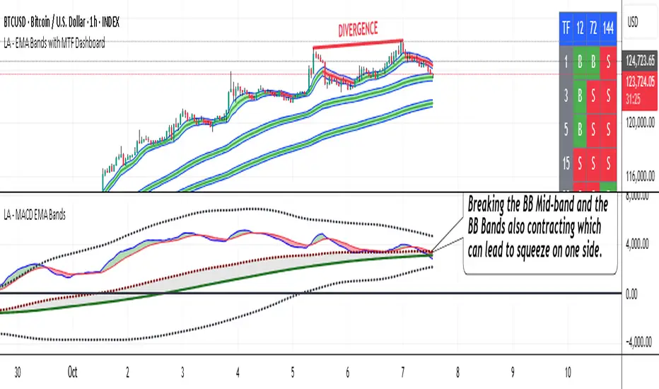
LA - MACD EMA BandsOverview of the "LA - MACD EMA Bands" Indicator
For Better view, use this indicator along with "LA - EMA Bands with MTF Dashboard"
The "LA - MACD EMA Bands" is a custom technical indicator written in Pine Script v6 for TradingView. It builds on the traditional Moving Average Convergence Divergence (MACD) oscillator by incorporating additional smoothing via Exponential Moving Averages (EMAs) and Bollinger Bands (BB) applied directly to the MACD line. This creates a multi-layered momentum and volatility tool displayed in a separate pane below the price chart (not overlaid on the price itself).
The indicator allows for customization, such as selecting a different timeframe (for multi-timeframe analysis) and adjusting period lengths. It fetches data from the specified timeframe using request.security with lookahead enabled to avoid repainting issues. The core idea is to provide insights into momentum trends, crossovers, and volatility expansions/contractions in the MACD's behavior, making it suitable for identifying potential trend reversals, continuations, or ranging markets.
Unlike a standard MACD, which focuses primarily on momentum via a single line, signal line, and histogram, this version emphasizes longer-term smoothing and volatility boundaries. It uses visual fills between lines to highlight bullish/bearish conditions, aiding quick interpretation. Below, I'll break down each component, its calculation, visual representation, and practical uses.
Detailed Breakdown of Each Component and Its Uses
MACD Line (Blue Line, Labeled 'MACD Line')
Calculation: This is the core MACD value, computed as the difference between a fast EMA (default length 12) and a slow EMA (default length 144) of the input source (default: close price). The EMAs are calculated on data from the selected timeframe.
Visuals: Plotted as a solid blue line.
Uses:
Measures momentum: When above zero, it indicates bullish momentum (prices rising faster in the short term); below zero, bearish momentum.
Trend identification: Rising MACD suggests strengthening uptrends; falling suggests downtrends.
Divergence spotting: Compare with price action—e.g., if price makes higher highs but MACD makes lower highs, it signals potential bearish reversal (and vice versa for bullish divergence).
In trading: Often used for entry/exit signals when crossing the zero line or other lines in the indicator.
MACD EMA (Red Line, Labeled 'MACD EMA')
Calculation: A 12-period EMA applied to the MACD Line itself.
Visuals: Plotted as a solid red line.
Uses:
Acts as a signal line for the MACD, smoothing out short-term noise.
Crossover signals: When the MACD Line crosses above the MACD EMA, it can signal a bullish buy opportunity; crossing below suggests a bearish sell.
Trend confirmation: Helps filter false signals in choppy markets by requiring confirmation from this slower-moving average.
In trading: Useful for momentum-based strategies, like entering trades on crossovers in alignment with the overall trend.
Fill Between MACD Line and MACD EMA (Green/Red Shaded Area, Titled 'MACD Fill')
Calculation: The area between the MACD Line and MACD EMA is filled with color based on their relative positions.
Color Logic: Green (with 57% transparency) if MACD Line > MACD EMA (bullish); red if MACD Line < MACD EMA (bearish).
Visuals: Semi-transparent fill for easy visibility without overwhelming the lines.
Uses:
Quick visual cue for momentum shifts: Green areas highlight bullish phases; red for bearish.
Enhances readability: Makes crossovers more apparent at a glance, especially in fast-moving markets.
In trading: Can be used to time entries/exits or as a filter (e.g., only take long trades in green zones).
Bollinger Bands on MACD (BB Upper: Black Dotted, BB Basis: Maroon Dotted, BB Lower: Black Dotted)
Calculation: Bollinger Bands applied to the MACD Line.
BB Basis: 144-period EMA of the MACD Line.
BB Standard Deviation: 144-period stdev of the MACD Line.
BB Upper: BB Basis + (2.0 * BB Stdev)
BB Lower: BB Basis - (2.0 * BB Stdev)
Visuals: Upper and lower bands as black dotted lines; basis as maroon dotted
Uses:
Volatility measurement: Bands expand during high momentum volatility (strong trends) and contract during low volatility (ranging or consolidation).
Mean reversion: When MACD Line touches or exceeds the upper band, it may signal overbought conditions (potential sell); lower band for oversold (potential buy).
Squeeze detection: Narrow bands (squeeze) often precede big moves—watch for breakouts.
In trading: Combines momentum with volatility; e.g., a MACD Line breakout above the upper band could confirm a strong uptrend.
BB Basis EMA (Green Line, Labeled 'BB Basis EMA')
Calculation: A 72-period EMA applied to the BB Basis (which is already a 144-period EMA of the MACD Line).
Visuals: Solid green line.
Uses:
Further smoothing: Provides a longer-term view of the MACD's average behavior, reducing noise from the BB Basis.
Trend direction: Acts as a baseline for the BB system—above it suggests bullish bias in momentum volatility; below, bearish.
Crossover with BB Basis: Can signal shifts in volatility trends (e.g., BB Basis crossing above BB Basis EMA indicates increasing bullish volatility).
In trading: Useful for confirming longer-term trends or as a filter for BB-based signals.
Fill Between BB Basis and BB Basis EMA (Gray Shaded Area, Titled 'BB Basis Fill')
Calculation: The area between BB Basis and BB Basis EMA is filled.
Color Logic: Currently set to a constant semi-transparent gray regardless of position.
Visuals: Semi-transparent gray fill.
Uses:
Highlights divergence: Shows when the shorter-term BB Basis deviates from its longer-term EMA, indicating potential volatility shifts.
Visual aid for crossovers: Makes it easier to spot when BB Basis crosses its EMA.
In trading: Could be used to identify overextensions in volatility (e.g., wide gray areas might signal impending mean reversion).
Zero Line (Black Horizontal Line)
Calculation: A simple horizontal line at y=0.
Visuals: Solid black line.
Uses:
Reference point: Divides bullish (above) from bearish (below) territory for all MACD-related lines.
In trading: Crossovers of the zero line by the MACD Line or BB Basis can signal major trend changes.
How It Differs from a Normal MACD
A standard MACD (e.g., the built-in TradingView MACD with defaults 12/26/9) consists of:
MACD Line: EMA(12) - EMA(26).
Signal Line: EMA(MACD Line, 9).
Histogram: MACD Line - Signal Line (bars showing convergence/divergence).
Key differences in "LA - MACD EMA Bands":
Periods: Uses a much longer slow EMA (144 vs. 26), making it more sensitive to long-term trends but less reactive to short-term price action. The MACD EMA is 12 periods (vs. 9), further emphasizing smoothing.
No Histogram: Replaces the histogram with fills and bands for visual emphasis on crossovers and volatility.
Added Bollinger Bands: Applies BB directly to the MACD Line (with a long 144-period basis), introducing volatility analysis absent in standard MACD. This helps detect "squeezes" or expansions in momentum.
Additional EMA Layer: The BB Basis EMA (72-period) adds a secondary smoothing level to the BB system, providing a hierarchical view of momentum (short-term MACD → mid-term BB → long-term EMA).
Multi-Timeframe Support: Built-in option for higher timeframes, unlike basic MACD.
Focus: Standard MACD is purely momentum-focused; this version integrates volatility (via BB) and multi-layer smoothing, making it better for trend-following in volatile markets but potentially overwhelming for beginners.
Overall, this indicator transforms the MACD from a simple oscillator into a comprehensive momentum-volatility hybrid, reducing false signals in trending markets but introducing lag.
Overall Pros and Cons
Pros:
Enhanced Visualization: Fills and bands make trends, crossovers, and volatility easier to spot without needing multiple indicators.
Reduced Noise: Longer periods (144, 72) smooth out whipsaws, ideal for swing or position trading in trending assets like stocks or forex.
Volatility Integration: BB adds a dimension not in standard MACD, helping identify breakouts or consolidations.
Customizable: Inputs for timeframes and lengths allow adaptation to different assets/timeframes.
Multi-Layered Insights: Combines short-term signals (MACD crossovers) with long-term confirmation (BB EMA), improving signal reliability.
Cons:
Lagging Nature: Long periods (e.g., 144) delay signals, missing early entries in fast markets or leading to late exits.
Complexity: Multiple lines and fills can clutter the pane, requiring experience to interpret; beginners might misread it.
Potential Overfitting: Custom periods (12/144/12/144/72) may work well on historical data but underperform in live trading without backtesting.
No Built-in Alerts/Signals: Relies on visual interpretation; users must manually set alerts for crossovers.
Resource Intensive: On lower timeframes or with lookahead, it might slow chart loading on Trading View.
This indicator shines in strategies combining momentum and volatility, like trend-following with BB squeezes, but test it on your assets (e.g., via backtesting) to ensure it fits your style.
For Better view, use this indicator along with "LA - EMA Bands with MTF Dashboard"
在腳本中搜尋"12月4号是什么星座"
Swing Guardrail — 30-sec Midterm Check (EBITDA Margin & EV/EBITDWhat it does
Before a short-term swing entry, this indicator right-sizes positions by a quick midterm (3–12m) durability screen using two fundamentals:
EBITDA Margin (TTM) → earning power / operational resilience
EV/EBITDA (TTM) → price tag vs earning capacity (payback feel)
A high-contrast table (top-right) shows both metrics and a verdict:
PASS — both meet thresholds → normal size
HALF — only one meets → reduce size
FAIL — neither meets → avoid
Why check “midterm” for a short-term trade?
Short swings still face earnings/news gaps, failed breakouts, and regime shifts. Names with weak margins or stretched valuation tend to break faster and deeper. A 30-sec durability check helps you:
Filter fragile setups (avoid expensive + weakening names)
Stabilize drawdowns (size down when quality/price don’t align)
Keep timing unchanged while improving risk-adjusted returns
Inputs (defaults)
Min EBITDA Margin % (TTM): 8%
Max EV/EBITDA (TTM): 12
Dark chart? High-contrast colors
How to use with a swing system
Get your entry from price/volume (e.g., Ichimoku cloud break, Kijun reclaim, Tenkan>Kijun; or your A/B/C rules).
Run this check only to set size (not timing).
Optional alerts: Once per bar close for PASS / HALF / FAIL.
Size mapping & event guard
PASS → 100% of your planned size
HALF → ~50% size / tighter stops
FAIL → watchlist only
If earnings < ~10 JP business days, drop one tier; ≤3 days → avoid.
Sector guides (tweak as needed)
Software/Internet: Margin ≥ 15%, EV/EBITDA ≤ 18
Industrials/Consumer: Margin ≥ 8%, EV/EBITDA ≤ 12
Retail: Margin ≥ 5–7%, EV/EBITDA ≤ 10–12
Edge cases / substitutions
Banks/Insurers/REITs or net-cash/negative EBITDA: EV/EBITDA may mislead → consider Net Debt/EBITDA or sector metrics (CET1/LTV/DSCR).
Sparse data / fresh listings: numbers may be NA until updates.
Notes & limitations
Data via request.financial() (TTM/most-recent). Some tickers/regions can show NA until fundamentals refresh.
This is a risk-screen / sizing tool, not a buy/sell signal.
Disclaimer
Educational use only. Not investment advice.
日本語
タイトル
スイング用ガードレール―中期“壊れにくさ”30秒チェック(EBITDAマージン & EV/EBITDA, TTM)
概要
短期スイングのエントリー前に、中期(3〜12か月)の耐久性を2指標で素早く確認し、ポジションサイズを決めるためのツールです。
EBITDAマージン(TTM):事業の稼ぐ力・体力
EV/EBITDA(TTM):その体力に対する“値札”(回収年数の感覚)
右上の高コントラスト表に数値と判定を表示:
PASS:両方クリア → 通常サイズ
HALF:片方のみ → サイズ半分
FAIL:両方NG → 見送り
なぜ短期でも“中期”を確認?
短期でも決算・ニュースのギャップ、ブレイク失敗、地合い転換は起きます。マージンが弱い/割高すぎる銘柄は崩れやすく、戻りも鈍い傾向。30秒の耐久性チェックで
脆いセットアップを回避
ドローダウンを平準化(サイズで吸収)
タイミングは変えずに、リスク調整後リターンの改善を狙えます。
入力(既定)
最低EBITDAマージン:8%
最大EV/EBITDA:12
黒背景向け:高コントラスト表示
使い方(スイング手法と併用)
まずは価格シグナル(一目の雲上抜け/基準線回復/転換線>基準線、またはA/B/Cルール)。
本インジの判定でサイズのみ決定(エントリーのタイミングは出しません)。
任意でバー確定アラート(PASS/HALF/FAIL)を設定。
サイズ目安 & イベント抑制
PASS:計画サイズ100%
HALF:約50%(ストップもタイトに)
FAIL:見送り
決算まで≦10営業日なら1段階サイズダウン、≦3営業日は原則見送り。
セクター目安(調整推奨)
ソフト/ネット:マージン 15%以上、EV/EBITDA 18以下
工業/一般消費:マージン 8%以上、EV/EBITDA 12以下
小売:マージン 5〜7%以上、EV/EBITDA 10〜12以下
例外・代替
銀行・保険・REIT/ネットキャッシュ・EBITDAマイナス:EV/EBITDAは適さない場合 → Net Debt/EBITDAやCET1/LTV/DSCR等で補助。
新規上場・データ薄:更新までNAのことあり。
注意
データは request.financial() を使用。更新前はNAの可能性。
本ツールはリスク確認/サイズ調整用で、売買シグナルではありません。
免責
情報提供のみ。投資判断は自己責任で。
FUMO 200 MagnetWhat it does
FUMO Magnet measures how far price has stretched away from its long-term “magnet” — a blended EMA/SMA moving average (200 by default).
It plots a logarithmic deviation (optionally normalized) as an oscillator around zero.
Above 0** → price is above the magnet (stretched up)
Below 0** → price is below the magnet (stretched down)
Guide levels** highlight potential overbought/oversold zones
---
Why log deviation?
Log returns make extremes comparable across cycles and compress exponential trends — especially useful for BTC and other crypto assets.
Normalization modes further adjust the scale, keeping the oscillator readable on any chart.
---
Inputs
**Base**
* Source (default: Close)
* Base Length (default: 200 EMA/SMA)
* EMA vs SMA weight (%) — 0% = pure SMA, 100% = pure EMA, 50% = blended
* EMA smoothing of deviation — acts as a noise filter
**Normalization**
* None (Log Deviation) — raw log stretch in % terms
* Z-score — deviation in standard deviations (σ)
* Robust Z (MAD) — deviation vs median absolute deviation, resistant to outliers
* Tanh squash — smooth nonlinear squash of extremes for compact scale
* Normalization window (for Z / MAD)
* Tanh scale (lower = stronger squash)
* Clamp after normalization — hard cap at ±X
**Levels**
* Guide levels (Upper / Lower) — visual thresholds (default ±12)
* Zero line toggle
---
### How to read it
* **Trend bias**: sustained time above 0 = uptrend, below 0 = downtrend
* **Stretch / mean reversion**: the farther from 0, the higher the reversion risk
* **Cross-checks**: combine with structure (HH/HL, LH/LL), volume, or momentum (RSI, MACD)
---
### Recommended settings by timeframe
**Long-term (1D / 1W)**
* Normalization: None (Log Deviation)
* Base Length: 200
* EMA vs SMA weight: 50% (adjust 35–65% for faster/slower magnet)
* Deviation smoothing: 20 (10–30 range)
* Guide levels: ±12 to ±20
* Use case: cycle extremes, portfolio rebalancing, trim/add logic
**Swing (4H – 1D)**
* Normalization: Z-score
* Window: 200 (100–250)
* Smoothing: 14–20
* Guide levels: ±2σ to ±3σ
* Use case: stretched conditions across regimes; ±3σ is rare, often mean-reverts
**Intraday / Active swing (1H – 4H)**
* Normalization: Robust Z (MAD)
* Window: 200 (150 for faster response)
* Smoothing: 10–16
* Guide levels: ±3 to ±4 (robust units)
* Use case: handles spikes better than σ, fewer false overbought/oversold signals
**Scalping / Universal readability (15m – 1H)**
* Normalization: Tanh squash
* Tanh scale: 6–10 (start with 8)
* Smoothing: 8–12
* Guide levels: ±8 to ±12
* Use case: compact panel across assets and timeframes; not % or σ, but visually consistent
---
### Optional
* Clamp: enable ±20 (or ±25) for strict bounded range (useful for public charts)
---
### Quick setups
**BTC Daily (“cycle view”)**
* Normalization: None
* Blend: 50%
* Smooth: 20
* Levels: ±12–15
**BTC 4H (“swing”)**
* Normalization: Z-score
* Window: 200
* Smooth: 16
* Levels: ±2.5σ to ±3σ
**Alts 1H (“volatile”)**
* Normalization: Robust Z (MAD)
* Window: 200
* Smooth: 12
* Levels: ±3.5 to ±4.5
**Mixed assets 15m (“compact panel”)**
* Normalization: Tanh squash
* Scale: 8
* Smooth: 10
* Levels: ±8–12
* Clamp: ±20
Meta-LR ForecastThis indicator builds a forward-looking projection from the current bar by combining twelve time-compressed “mini forecasts.” Each forecast is a linear-regression-based outlook whose contribution is adaptively scaled by trend strength (via ADX) and normalized to each timeframe’s own volatility (via that timeframe’s ATR). The result is a 12-segment polyline that starts at the current price and extends one bar at a time into the future (1× through 12× the chart’s timeframe). Alongside the plotted path, the script computes two summary measures:
* Per-TF Bias% — a directional efficiency × R² score for each micro-forecast, expressed as a percent.
* Meta Bias% — the same score, but applied to the final, accumulated 12-step path. It summarizes how coherent and directional the combined projection is.
This tool is an indicator, not a strategy. It does not place orders. Nothing here is trade advice; it is a visual, quantitative framework to help you assess directional bias and trend context across a ladder of timeframe multiples.
The core engine fits a simple least-squares line on a normalized price series for each small forecast horizon and extrapolates one bar forward. That “trend” forecast is paired with its mirror, an “anti-trend” forecast, constructed around the current normalized price. The model then blends between these two wings according to current trend strength as measured by ADX.
ADX is transformed into a weight (w) in using an adaptive band centered on the rolling mean (μ) with width derived from the standard deviation (σ) of ADX over a configurable lookback. When ADX is deeply below the lower band, the weight approaches -1, favoring anti-trend behavior. Inside the flat band, the weight is near zero, producing neutral behavior. Clearly above the upper band, the weight approaches +1, favoring a trend-following stance. The transitions between these regions are linear so the regime shift is smooth rather than abrupt.
You can shape how quickly the model commits to either wing using two exponents. One exponent controls how aggressively positive weights lean into the trend forecast; the other controls how aggressively negative weights lean into the anti-trend forecast. Raising these exponents makes the response more gradual; lowering them makes the shift more decisive. An optional switch can force full anti-trend behavior when ADX registers a deep-low condition far below the lower tail, if you prefer a categorical stance in very flat markets.
A key design choice is volatility normalization. Every micro-forecast is computed in ATR units of its own timeframe. The script fetches that timeframe’s ATR inside each security call and converts normalized outputs back to price with that exact ATR. This avoids scaling higher-timeframe effects by the chart ATR or by square-root time approximations. Using “ATR-true” for each timeframe keeps the cross-timeframe accumulation consistent and dimensionally correct.
Bias% is defined as directional efficiency multiplied by R², expressed as a percent. Directional efficiency captures how much net progress occurred relative to the total path length; R² captures how well the path aligns with a straight line. If price meanders without net progress, efficiency drops; if the variation is well-explained by a line, R² rises. Multiplying the two penalizes choppy, low-signal paths and rewards sustained, coherent motion.
The forward path is built by converting each per-timeframe Bias% into a small ATR-sized delta, then cumulatively adding those deltas to form a 12-step projection. This produces a polyline anchored at the current close and stepping forward one bar per timeframe multiple. Segment color flips by slope, allowing a quick read of the path’s direction and inflection.
Inputs you can tune include:
* Max Regression Length. Upper bound for each micro-forecast’s regression window. Larger values smooth the trend estimate at the cost of responsiveness; smaller values react faster but can add noise.
* Price Source. The price series analyzed (for example, close or typical price).
* ADX Length. Period used for the DMI/ADX calculation.
* ATR Length (normalization). Window used for ATR; this is applied per timeframe inside each security call.
* Band Lookback (for μ, σ). Lookback used to compute the adaptive ADX band statistics. Larger values stabilize the band; smaller values react more quickly.
* Flat half-width (σ). Width of the neutral band on both sides of μ. Wider flats spend more time neutral; narrower flats switch regimes more readily.
* Tail width beyond flat (σ). Distance from the flat band edge to the extreme trend/anti-trend zone. Larger tails create a longer ramp; smaller tails reach extremes sooner.
* Polyline Width. Visual thickness of the plotted segments.
* Negative Wing Aggression (anti-trend). Exponent shaping for negative weights; higher values soften the tilt into mean reversion.
* Positive Wing Aggression (trend). Exponent shaping for positive weights; lower values make trend commitment stronger and sooner.
* Force FULL Anti-Trend at Deep-Low ADX. Optional hard switch for extremely low ADX conditions.
On the chart you will see:
* A 12-segment forward polyline starting from the current close to bar\_index + 1 … +12, with green segments for up-steps and red for down-steps.
* A small label at the latest bar showing Meta Bias% when available, or “n/a” when insufficient data exists.
Interpreting the readouts:
* Trend-following contexts are characterized by ADX above the adaptive upper band, pushing w toward +1. The blended forecast leans toward the regression extrapolation. A strongly positive Meta Bias% in this environment suggests directional alignment across the ladder of timeframes.
* Mean-reversion contexts occur when ADX is well below the lower tail, pushing w toward -1 (or forcing anti-trend if enabled). After a sharp advance, a negative Meta Bias% may indicate the model projects pullback tendencies.
* Neutral contexts occur when ADX sits inside the flat band; w is near zero, the blended forecast remains close to current price, and Meta Bias% tends to hover near zero.
These are analytical cues, not rules. Always corroborate with your broader process, including market structure, time-of-day behavior, liquidity conditions, and risk limits.
Practical usage patterns include:
* Momentum confirmation. Combine a rising Meta Bias% with higher-timeframe structure (such as higher highs and higher lows) to validate continuation setups. Treat the 12th step’s distance as a coarse sense of potential room rather than as a target.
* Fade filtering. If you prefer fading extremes, require ADX to be near or below the lower ramp before acting on counter-moves, and avoid fades when ADX is decisively above the upper band.
* Position planning. Because per-step deltas are ATR-scaled, the path’s vertical extent can be mentally mapped to typical noise for the instrument, informing stop distance choices. The script itself does not compute orders or size.
* Multi-timeframe alignment. Each step corresponds to a clean multiple of your chart timeframe, so the polyline visualizes how successively larger windows bias price, all referenced to the current bar.
House-rules and repainting disclosures:
* Indicator, not strategy. The script does not execute, manage, or suggest orders. It displays computed paths and bias scores for analysis only.
* No performance claims. Past behavior of any measure, including Meta Bias%, does not guarantee future results. There are no assurances of profitability.
* Higher-timeframe updates. Values obtained via security for higher-timeframe series can update intrabar until the higher-timeframe bar closes. The forward path and Meta Bias% may change during formation of a higher-timeframe candle. If you need confirmed higher-timeframe inputs, consider reading the prior higher-timeframe value or acting only after the higher-timeframe close.
* Data sufficiency. The model requires enough history to compute ATR, ADX statistics, and regression windows. On very young charts or illiquid symbols, parts of the readout can be unavailable until sufficient data accumulates.
* Volatility regimes. ATR normalization helps compare across timeframes, but unusual volatility regimes can make the path look deceptively flat or exaggerated. Judge the vertical scale relative to your instrument’s typical ATR.
Tuning tips:
* Stability versus responsiveness. Increase Max Regression Length to steady the micro-forecasts but accept slower response. If you lower it, consider slightly increasing Band Lookback so regime boundaries are not too jumpy.
* Regime bands. Widen the flat half-width to spend more time neutral, which can reduce over-trading tendencies in chop. Shrink the tail width if you want the model to commit to extremes sooner, at the cost of more false swings.
* Wing shaping. If anti-trend behavior feels too abrupt at low ADX, raise the negative wing exponent. If you want trend bias to kick in more decisively at high ADX, lower the positive wing exponent. Small changes have large effects.
* Forced anti-trend. Enable the deep-low option only if you explicitly want a categorical “markets are flat, fade moves” policy. Many users prefer leaving it off to keep regime decisions continuous.
Troubleshooting:
* Nothing plots or the label shows “n/a.” Ensure the chart has enough history for the ADX band statistics, ATR, and the regression windows. Exotic or illiquid symbols with missing data may starve the higher-timeframe computations. Try a more liquid market or a higher timeframe.
* Path flickers or shifts during the bar. This is expected when any higher-timeframe input is still forming. Wait for the higher-timeframe close for fully confirmed behavior, or modify the code to read prior values from the higher timeframe.
* Polyline looks too flat or too steep. Check the chart’s vertical scale and recent ATR regime. Adjust Max Regression Length, the wing exponents, or the band widths to suit the instrument.
Integration ideas for manual workflows:
* Confluence checklist. Use Meta Bias% as one of several independent checks, alongside structure, session context, and event risk. Act only when multiple cues align.
* Stop and target thinking. Because deltas are ATR-scaled at each timeframe, benchmark your proposed stops and targets against the forward steps’ magnitude. Stops that are much tighter than the prevailing ATR often sit inside normal noise.
* Session context. Consider session hours and microstructure. The same ADX value can imply different tradeability in different sessions, particularly in index futures and FX.
This indicator deliberately avoids:
* Fixed thresholds for buy or sell decisions. Markets vary and fixed numbers invite overfitting. Decide what constitutes “high enough” Meta Bias% for your market and timeframe.
* Automatic risk sizing. Proper sizing depends on account parameters, instrument specifications, and personal risk tolerance. Keep that decision in your risk plan, not in a visual bias tool.
* Claims of edge. These measures summarize path geometry and trend context; they do not ensure a tradable edge on their own.
Summary of how to think about the output:
* The script builds a 12-step forward path by stacking linear-regression micro-forecasts across increasing multiples of the chart timeframe.
* Each micro-forecast is blended between trend and anti-trend using an adaptive ADX band with separate aggression controls for positive and negative regimes.
* All computations are done in ATR-true units for each timeframe before reconversion to price, ensuring dimensional consistency when accumulating steps.
* Bias% (per-timeframe and Meta) condenses directional efficiency and trend fidelity into a compact score.
* The output is designed to serve as an analytical overlay that helps assess whether conditions look trend-friendly, fade-friendly, or neutral, while acknowledging higher-timeframe update behavior and avoiding prescriptive trade rules.
Use this tool as one component within a disciplined process that includes independent confirmation, event awareness, and robust risk management.

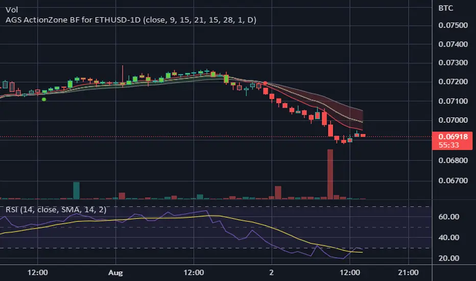
CDC ActionZone BF for ETHUSD-1D © PRoSkYNeT-EE
Based on improvements from "Kitti-Playbook Action Zone V.4.2.0.3 for Stock Market"
Based on improvements from "CDC Action Zone V3 2020 by piriya33"
Based on Triple MACD crossover between 9/15, 21/28, 15/28 for filter error signal (noise) from CDC ActionZone V3
MACDs generated from the execution of millions of times in the "Brute Force Algorithm" to backtest data from the past 5 years. ( 2017-08-21 to 2022-08-01 )
Released 2022-08-01
***** The indicator is used in the ETHUSD 1 Day period ONLY *****
Recommended Stop Loss : -4 % (execute stop Loss after candlestick has been closed)
Backtest Result ( Start $100 )
Winrate 63 % (Win:12, Loss:7, Total:19)
Live Days 1,806 days
B : Buy
S : Sell
SL : Stop Loss
2022-07-19 07 - 1,542 : B 6.971 ETH
2022-04-13 07 - 3,118 : S 8.98 % $10,750 12,7,19 63 %
2022-03-20 07 - 2,861 : B 3.448 ETH
2021-12-03 07 - 4,216 : SL -8.94 % $9,864 11,7,18 61 %
2021-11-30 07 - 4,630 : B 2.340 ETH
2021-11-18 07 - 3,997 : S 13.71 % $10,832 11,6,17 65 %
2021-10-05 07 - 3,515 : B 2.710 ETH
2021-09-20 07 - 2,977 : S 29.38 % $9,526 10,6,16 63 %
2021-07-28 07 - 2,301 : B 3.200 ETH
2021-05-20 07 - 2,769 : S 50.49 % $7,363 9,6,15 60 %
2021-03-30 07 - 1,840 : B 2.659 ETH
2021-03-22 07 - 1,681 : SL -8.29 % $4,893 8,6,14 57 %
2021-03-08 07 - 1,833 : B 2.911 ETH
2021-02-26 07 - 1,445 : S 279.27 % $5,335 8,5,13 62 %
2020-10-13 07 - 381 : B 3.692 ETH
2020-09-05 07 - 335 : S 38.43 % $1,407 7,5,12 58 %
2020-07-06 07 - 242 : B 4.199 ETH
2020-06-27 07 - 221 : S 28.49 % $1,016 6,5,11 55 %
2020-04-16 07 - 172 : B 4.598 ETH
2020-02-29 07 - 217 : S 47.62 % $791 5,5,10 50 %
2020-01-12 07 - 147 : B 3.644 ETH
2019-11-18 07 - 178 : S -2.73 % $536 4,5,9 44 %
2019-11-01 07 - 183 : B 3.010 ETH
2019-09-23 07 - 201 : SL -4.29 % $551 4,4,8 50 %
2019-09-18 07 - 210 : B 2.740 ETH
2019-07-12 07 - 275 : S 63.69 % $575 4,3,7 57 %
2019-05-03 07 - 168 : B 2.093 ETH
2019-04-28 07 - 158 : S 29.51 % $352 3,3,6 50 %
2019-02-15 07 - 122 : B 2.225 ETH
2019-01-10 07 - 125 : SL -6.02 % $271 2,3,5 40 %
2018-12-29 07 - 133 : B 2.172 ETH
2018-05-22 07 - 641 : S 5.95 % $289 2,2,4 50 %
2018-04-21 07 - 605 : B 0.451 ETH
2018-02-02 07 - 922 : S 197.42 % $273 1,2,3 33 %
2017-11-11 07 - 310 : B 0.296 ETH
2017-10-09 07 - 297 : SL -4.50 % $92 0,2,2 0 %
2017-10-07 07 - 311 : B 0.309 ETH
2017-08-22 07 - 310 : SL -4.02 % $96 0,1,1 0 %
2017-08-21 07 - 323 : B 0.310 ETH
Bar Balance [LucF]Bar Balance extracts the number of up, down and neutral intrabars contained in each chart bar, revealing information on the strength of price movement. It can display stacked columns representing raw up/down/neutral intrabar counts, or an up/down balance line which can be calculated and visualized in many different ways.
WARNING: This is an analysis tool that works on historical bars only. It does not show any realtime information, and thus cannot be used to issue alerts or for automated trading. When realtime bars elapse, the indicator will require a browser refresh, a change to its Inputs or to the chart's timeframe/symbol to recalculate and display information on those elapsed bars. Once a trader understands this, the indicator can be used advantageously to make discretionary trading decisions.
Traders used to work with my Delta Volume Columns Pro will feel right at home in this indicator's Inputs . It has lots of options, allowing it to be used in many different ways. If you value the bar balance information this indicator mines, I hope you will find the time required to master the use of Bar Balance well worth the investment.
█ OVERVIEW
The indicator has two modes: Columns and Line .
Columns
• In Columns mode you can display stacked Up/Down/Neutral columns.
• The "Up" section represents the count of intrabars where `close > open`, "Down" where `close < open` and "Neutral" where `close = open`.
• The Up section always appears above the centerline, the Down section below. The Neutral section overlaps the centerline, split halfway above and below it.
The Up and Down sections start where the Neutral section ends, when there is one.
• The Up and Down sections can be colored independently using 7 different methods.
• The signal line plotted in Line mode can also be displayed in Columns mode.
Line
• Displays a single balance line using a zero centerline.
• A variable number of independent methods can be used to calculate the line (6), determine its color (5), and color the fill (5).
You can thus evaluate the state of 3 different components with this single line.
• A "Divergence Levels" feature will use the line to automatically draw expanding levels on divergence events.
Features available in both modes
• The color of all components can be selected from 15 base colors, with 16 gradient levels used for each base color in the indicator's gradients.
• A zero line can show a 6-state aggregate value of the three main volume balance modes.
• The background can be colored using any of 5 different methods.
• Chart bars can be colored using 5 different methods.
• Divergence and large neutral count ratio events can be shown in either Columns or Line mode, calculated in one of 4 different methods.
• Markers on 6 different conditions can be displayed.
█ CONCEPTS
Intrabar inspection
Intrabar inspection means the indicator looks at lower timeframe bars ( intrabars ) making up a given chart bar to gather its information. If your chart is on a 1-hour timeframe and the intrabar resolution determined by the indicator is 5 minutes, then 12 intrabars will be analyzed for each chart bar and the count of up/down/neutral intrabars among those will be tallied.
Bar Balances and calculation methods
The indicator uses a variety of methods to evaluate bar balance and to derive other calculations from them:
1. Balance on Bar : Uses the relative importance of instant Up and Down counts on the bar.
2. Balance Averages : Uses the difference between the EMAs of Up and Down counts.
3. Balance Momentum : Starts by calculating, separately for both Up and Down counts, the difference between the same EMAs used in Balance Averages and an SMA of double the period used for the EMAs. These differences are then aggregated and finally, a bounded momentum of that aggregate is calculated using RSI.
4. Markers Bias : It sums the bull/bear occurrences of the four previous markers over a user-defined period (the default is 14).
5. Combined Balances : This is the aggregate of the instant bull/bear bias of the three main bar balances.
6. Dual Up/Down Averages : This is a display mode showing the EMA calculated for each of the Up and Down counts.
Interpretation of neutral intrabars
What do neutral intrabars mean? When price does not change during a bar, it can be because there is simply no interest in the market, or because of a perfect balance between buyers and sellers. The latter being more improbable, Bar Balance assumes that neutral bars reveal a lack of interest, which entails uncertainty. That is the reason why the option is provided to interpret ratios of neutral intrabars greater than 50% as divergences. It is also the rationale behind the option to dampen signal lines on the inverse ratio of neutral intrabars, so that zero intrabars do not affect the signal, and progressively larger proportions of neutral intrabars will reduce the signal's amplitude, as the balance calcs using the up/down counts lose significance. The impact of the dampening will vary with markets. Weaker markets such as cryptos will often contain greater numbers of neutral intrabars, so dampening the Line in that sector will have a greater impact than in more liquid markets.
█ FEATURES
1 — Columns
• While the size of the Up/Down columns always represents their respective importance on the bar, their coloring mode is independent. The default setup uses a standard coloring mode where the Up/Down columns over/under the zero line are always in the bull/bear color with a higher intensity for the winning side. Six other coloring modes allow you to pack more information in the columns. When choosing to color the top columns using a bull/bear gradient on Balance Averages, for example, you will end up with bull/bear colored tops. In order for the color of the bottom columns to continue to show the instant bar balance, you can then choose the "Up/Down Ratio on Bar — Dual Solid Colors" coloring mode to make those bars the color of the winning side for that bar.
• Line mode shows only the line, but Columns mode allows displaying the line along with it. If the scale of the line is different than that of the scale of the columns, the line will often appear flat. Traders may find even a flat line useful as its bull/bear colors will be easily distinguishable.
2 — Line
• The default setup for Line mode uses a calculation on "Balance Momentum", with a fill on the longer-term "Balance Averages" and a line color based on the "Markers Bias". With the background set on "Line vs Divergence Levels" and the zero line on the hard-coded "Combined Bar Balances", you have access to five distinct sources of information at a glance, to which you can add divergences, divergences levels and chart bar coloring. This provides powerful potential in displaying bar balance information.
• When no columns are displayed, Line mode can show the full scale of whichever line you choose to calculate because the columns' scale no longer interferes with the line's scale.
• Note that when "Balance on Bar" is selected, the Neutral count is also displayed as a ratio of the balance line. This is the only instance where the Neutral count is displayed in Line mode.
• The "Dual Up/Down Averages" is an exception as it displays two lines: one average for the Up counts and another for the Down counts. This mode will be most useful when Columns are also displayed, as it provides a reference for the top and bottom columns.
3 — Zero Line
The zero line can be colored using two methods, both based on the Combined Balances, i.e., the aggregate of the instant bull/bear bias of the three main bar balances.
• In "Six-state Dual Color Gradient" mode, a dot appears on every bar. Its color reflects the bull/bear state of the Combined Balances, and the dot's brightness reflects the tally of balance biases.
• In "Dual Solid Colors (All Bull/All Bear Only)" a dot only appears when all three balances are either bullish or bearish. The resulting pattern is identical to that of Marker 1.
4 — Divergences
• Divergences are displayed as a small circle at the top of the scale. Four different types of divergence events can be detected. Divergences occur whenever the bull/bear bias of the method used diverges with the bar's price direction.
• An option allows you to include in divergence events instances where the count of neutral intrabars exceeds 50% of the total intrabar count.
• The divergence levels are dynamic levels that automatically build from the line's values on divergence events. On consecutive divergences, the levels will expand, creating a channel. This implementation of the divergence levels corresponds to my view that divergences indicate anomalies, hesitations, points of uncertainty if you will. It excludes any association of a pre-determined bullish/bearish bias to divergences. Accordingly, the levels merely take note of divergence events and mark those points in time with levels. Traders then have a reference point from which they can evaluate further movement. The bull/bear/neutral colors used to plot the levels are also congruent with this view in that they are determined by price's position relative to the levels, which is how I think divergences can be put to the most effective use.
5 — Background
• The background can show a bull/bear gradient on four different calculations. You can adjust its brightness to make its visual importance proportional to how you use it in your analysis.
6 — Chart bars
• Chart bars can be colored using five different methods.
• You have the option of emptying the body of bars where volume does not increase, as does my TLD indicator, the idea behind this being that movement on bars where volume does not increase is less relevant.
7 — Intrabar Resolution
You can choose between three modes. Two of them are automatic and one is manual:
a) Fast, Longer history, Auto-Steps (~12 intrabars) : Optimized for speed and deeper history. Uses an average minimum of 12 intrabars.
b) More Precise, Shorter History Auto-Steps (~24 intrabars) : Uses finer intrabar resolution. It is slower and provides less history. Uses an average minimum of 24 intrabars.
c) Fixed : Uses the fixed resolution of your choice.
Auto-Steps calculations vary for 24/7 and conventional markets in order to achieve the proper target of minimum intrabars.
You can choose to view the intrabar resolution currently used to calculate delta volume. It is the default.
The proper selection of the intrabar resolution is important. It must achieve maximal granularity to produce precise results while not unduly slowing down calculations, or worse, causing runtime errors.
8 — Markers
Six markers are available:
1. Combined Balances Agreement : All three Bar Balances are either bullish or bearish.
2. Up or Down % Agrees With Bar : An up marker will appear when the percentage of up intrabars in an up chart bar is greater than the specified percentage. Conditions mirror to down bars.
3. Divergence confirmations By Price : One of the four types of balance calculations can be used to detect divergences with price. Confirmations occur when the bar following the divergence confirms the balance bias. Note that the divergence events used here do not include neutral intrabar events.
4. Balance Transitions : Bull/bear transitions of the selected balance.
5. Markers Bias Transitions : Bull/bear transitions of the Markers Bias.
6. Divergence Confirmations By Line : Marks points where the line first breaches a divergence level.
Markers appear when the condition is detected, without delay. Since nothing is plotted in realtime, markers do not appear on the realtime bar.
9 — Settings
• Two modes can be selected to dampen the line on the ratio of neutral intrabars.
• A distinct weight can be attributed to the count of the latter half of intrabars, on the assumption that later intrabars may be more important in determining the outcome of chart bars.
• Allows control over the periods of the different moving averages used in calculations.
• The default periods used for the various calculations define the following hierarchy from slow to fast:
Balance Averages: 50,
Balance Momentum: 20,
Dual Up/Down Averages: 20,
Marker Bias: 10.
█ LIMITATIONS
• This script uses a special characteristic of the `security()` function allowing the inspection of intrabars—which is not officially supported by TradingView.
• The method used does not work on the realtime bar—only on historical bars.
• The indicator only works on some chart resolutions: 3, 5, 10, 15 and 30 minutes, 1, 2, 4, 6, and 12 hours, 1 day, 1 week and 1 month. The script’s code can be modified to run on other resolutions, but chart resolutions must be divisible by the lower resolution used for intrabars and the stepping mechanism could require adaptation.
• When using the "Line vs Divergence Levels — Dual Color Gradient" color mode to fill the line, background or chart bars, keep in mind that a line calculation mode must be defined for it to work, as it determines gradients on the movement of the line relative to divergence levels. If the line is hidden, it will not work.
• When the difference between the chart’s resolution and the intrabar resolution is too great, runtime errors will occur. The Auto-Steps selection mechanisms should avoid this.
• Alerts do not work reliably when `security()` is used at intrabar resolutions. Accordingly, no alerts are configured in the indicator.
• The color model used in the indicator provides for fancy visuals that come at a price; when you change values in Inputs , it can take 20 seconds for the changes to materialize. Luckily, once your color setup is complete, the color model does not have a large performance impact, as in normal operation the `security()` calls will become the most important factor in determining response time. Also, once in a while a runtime error will occur when you change inputs. Just making another change will usually bring the indicator back up.
█ RAMBLINGS
Is this thing useful?
I'll let you decide. Bar Balance acts somewhat like an X-Ray on bars. The intrabars it analyzes are no secret; one can simply change the chart's resolution to see the same intrabars the indicator uses. What the indicator brings to traders is the precise count of up/down/neutral intrabars and, more importantly, the calculations it derives from them to present the information in a way that can make it easier to use in trading decisions.
How reliable is Bar Balance information?
By the same token that an up bar does not guarantee that more up bars will follow, future price movements cannot be inferred from the mere count of up/down/neutral intrabars. Price movement during any chart bar for which, let's say, 12 intrabars are analyzed, could be due to only one of those intrabars. One can thus easily see how only relying on bar balance information could be very misleading. The rationale behind Bar Balance is that when the information mined for multiple chart bars is aggregated, it can provide insight into the history behind chart bars, and thus some bias as to the strength of movements. An up chart bar where 11/12 intrabars are also up is assumed to be stronger than the same up bar where only 2/12 intrabars are up. This logic is not bulletproof, and sometimes Bar Balance will stray. Also, keep in mind that balance lines do not represent price momentum as RSI would. Bar Balance calculations have no idea where price is. Their perspective, like that of any historian, is very limited, constrained that it is to the narrow universe of up/down/neutral intrabar counts. You will thus see instances where price is moving up while Balance Momentum, for example, is moving down. When Bar Balance performs as intended, this indicates that the rally is weakening, which does necessarily imply that price will reverse. Occasionally, price will merrily continue to advance on weakening strength.
Divergences
Most of the divergence detection methods used here rely on a difference between the bias of a calculation involving a multi-bar average and a given bar's price direction. When using "Bar Balance on Bar" however, only the bar's balance and price movement are used. This is the default mode.
As usual, divergences are points of interest because they reveal imbalances, which may or may not become turning points. I do not share the overwhelming enthusiasm traders have for the purported ability of bullish/bearish divergences to indicate imminent reversals.
Superfluity
In "The Bed of Procrustes", Nassim Nicholas Taleb writes: To bankrupt a fool, give him information . Bar Balance can display lots of information. While learning to use a new indicator inevitably requires an adaptation period where we put it through its paces and try out all its options, once you have become used to Bar Balance and decide to adopt it, rigorously eliminate the components you don't use and configure the remaining ones so their visual prominence reflects their relative importance in your analysis. I tried to provide flexible options for traders to control this indicator's visuals for that exact reason—not for window dressing.
█ NOTES
For traders
• To avoid misleading traders who don't read script descriptions, the indicator shows nothing in the realtime bar.
• The Data Window shows key values for the indicator.
• All gradients used in this indicator determine their brightness intensities using advances/declines in the signal—not their relative position in a fixed scale.
• Note that because of the way gradients are optimized internally, changing their brightness will sometimes require bringing down the value a few steps before you see an impact.
• Because this indicator does not use volume, it will work on all markets.
For coders
• For those interested in gradients, this script uses an advanced version of the Advance/Decline gradient function from the PineCoders Color Gradient (16 colors) Framework . It allows more precise control over the range, steps and min/max values of the gradients.
• I use the PineCoders Coding Conventions for Pine to write my scripts.
• I used functions modified from the PineCoders MTF Selection Framework for the selection of timeframes.
█ THANKS TO:
— alexgrover who helped me think through the dampening method used to attenuate signal lines on high ratios of neutral intrabars.
— A guy called Kuan who commented on a Backtest Rookies presentation of their Volume Profile indicator . The technique I use to inspect intrabars is derived from Kuan's code.
— theheirophant , my partner in the exploration of the sometimes weird abysses of `security()`’s behavior at intrabar resolutions.
— midtownsk8rguy , my brilliant companion in mining the depths of Pine graphics. He is also the co-author of the PineCoders Color Gradient Frameworks .

Monthly Color Marker V4
## 📊 Monthly Color Marker - Historical Month Highlighting
### Overview
A unique indicator that allows rapid identification of all monthly candles from a specific month across multiple years. The indicator marks candles with different colors based on their direction (bullish/bearish), enabling quick analysis of seasonal patterns and cyclical behavior of stocks or assets.
### 🎯 Purpose
- **Identify Seasonal Patterns (Seasonality)** - Discover recurring trends in specific months
- **Quick Historical Analysis** - Visual representation of monthly performance over the years
- **Direction Recognition** - Instant understanding of whether a month tends to be bullish or bearish
- **Seasonal Trading Planning** - Build strategies based on cyclical patterns
### ⚙️ Adjustable Parameters
1. **Month to Mark (1-12)**
- Select the desired month for analysis
- 1 = January, 2 = February... 12 = December
- Default: 11 (November)
2. **Years Back (1-50)**
- Determines how many years back to scan
- Recommended: 10-25 years for statistically reliable data
- Default: 25 years
3. **Bullish Candle Color**
- Color for marking bullish candles (close > open)
- Default: Green
- Customizable to your personal color scheme
4. **Bearish Candle Color**
- Color for marking bearish candles (close < open)
- Default: Red
- Customizable to your personal color scheme
5. **Show Current Year**
- Whether to include the current month in the marking
- Useful when the month hasn't finished yet
- Default: Yes
### 📈 How to Use the Indicator
#### Step 1: Adding to Chart
1. Switch to **Monthly timeframe** - Required!
2. Add the indicator to your chart
3. Select the month you want to analyze
#### Step 2: Initial Analysis
- **Count green vs red candles** - What's the ratio?
- **Look for patterns** - Are there years where the month always rises/falls?
- **Identify outliers** - Years where behavior was different
#### Step 3: Making Decisions
- **Mostly green** → Statistically, the month tends to rise
- **Mostly red** → Statistically, the month tends to fall
- **Mixed** → No clear seasonal pattern
### 💡 Usage Examples
**Example 1: "Santa Claus Rally"**
- Select month 12 (December)
- Check if there are mostly green candles
- If yes, this confirms the well-known year-end rally effect
**Example 2: "September Effect"**
- Select month 9 (September)
- Historically, September is considered a weak month
- Do the data support this for this stock?
**Example 3: Quarterly Earnings**
- Identify which month earnings are released
- Check the historical response
- Plan entry/exit accordingly
### 🔍 Combining with Other Indicators
This indicator works excellently with:
- **Historical Monthly Levels** (the first indicator) - Identify nearby price levels
- **Volume Profile** - Check volume during those months
- **RSI/MACD** - Identify momentum strength in specific months
### ⚠️ Important Notes
1. **Must use Monthly timeframe!** The indicator won't work correctly on other timeframes
2. **Statistical Sample** - More years = more reliable analysis
3. **Not a Guarantee** - Past performance doesn't guarantee future results, use additional analysis
4. **Adjust Colors** - If hard to see, change colors in settings
### 🎨 Tips for Optimal Experience
- **Zoom Out** - See more years at a glance
- **Clean Chart** - Remove unnecessary indicators for clear analysis
- **Compare Stocks** - Check multiple stocks for the same month
- **Document Findings** - Take screenshots and save insights for future reference
### 📊 Recommended Statistics
After identifying an interesting month:
- Calculate success rate (green / total candles)
- Check average volatility
- Identify outlier years and investigate what happened
- Plan entry/exit strategy
### 🚀 Who Is This Indicator For?
✅ **Swing Traders** - Plan medium-term trades
✅ **Seasonal Investors** - Exploit cyclical patterns
✅ **Technical Analysts** - Understand historical behavior
✅ **Portfolio Managers** - Time entries and exits
---
### 📝 Summary
The Monthly Color Marker indicator is a powerful and easy-to-use tool for identifying seasonal patterns. The combination of clear visualization with flexible parameters makes it an essential tool for any trader seeking a statistical edge in the market.
**Recommendation:** Start with 25 years back, analyze 2-3 key months, and build a data-driven strategy.
---
**Version:** 4.0
**Compatibility:** Pine Script v5
**Timeframe:** Monthly only
**Author:** 954
## 📊 Monthly Color Marker - סימון חודשים היסטוריים
### תיאור כללי
אינדיקטור ייחודי המאפשר לזהות במהירות את כל הנרות החודשיים מחודש ספציפי לאורך השנים. האינדיקטור מסמן את הנרות בצבעים שונים בהתאם לכיוון התנועה (עלייה/ירידה), ומאפשר ניתוח מהיר של דפוסים עונתיים והתנהגות מחזורית של המניה או הנכס.
### 🎯 מטרת האינדיקטור
- **זיהוי דפוסים עונתיים (Seasonality)** - מציאת מגמות חוזרות בחודשים מסוימים
- **ניתוח היסטורי מהיר** - ראייה ויזואלית של ביצועי החודש לאורך השנים
- **זיהוי כיווניות** - הבנה מיידית האם החודש נוטה להיות שורי או דובי
- **תכנון מסחר עונתי** - בניית אסטרטגיות מבוססות מחזוריות
### ⚙️ פרמטרים מתכווננים
1. **חודש לסימון (1-12)**
- בחירת החודש הרצוי לניתוח
- 1 = ינואר, 2 = פברואר... 12 = דצמבר
- ברירת מחדל: 11 (נובמבר)
2. **שנים אחורה (1-50)**
- קובע כמה שנים אחורה לסרוק
- מומלץ: 10-25 שנים לקבלת תמונה סטטיסטית מהימנה
- ברירת מחדל: 25 שנים
3. **צבע נר עולה**
- צבע לסימון נרות שורים (close > open)
- ברירת מחדל: ירוק
- ניתן להתאים לסכמת הצבעים האישית
4. **צבע נר יורד**
- צבע לסימון נרות דוביים (close < open)
- ברירת מחדל: אדום
- ניתן להתאים לסכמת הצבעים האישית
5. **צבע את השנה הנוכחית**
- האם לכלול את החודש הנוכחי בסימון
- שימושי כאשר החודש טרם הסתיים
- ברירת מחדל: כן
### 📈 איך להשתמש באינדיקטור
#### שלב 1: הוספה לגרף
1. עבור לטיימפריים **חודשי (Monthly)** - חובה!
2. הוסף את האינדיקטור לגרף
3. בחר את החודש שאתה רוצה לנתח
#### שלב 2: ניתוח ראשוני
- **ספור נרות ירוקים מול אדומים** - מה היחס?
- **חפש דפוסים** - האם יש שנים שבהן החודש תמיד עולה/יורד?
- **זהה חריגים** - שנים שבהן ההתנהגות הייתה שונה
#### שלב 3: קבלת החלטות
- **רוב ירוקים** → סטטיסטית החודש נוטה לעלות
- **רוב אדומים** → סטטיסטית החודש נוטה לרדת
- **מעורב** → אין דפוס עונתי ברור
### 💡 דוגמאות שימוש
**דוגמה 1: "Santa Claus Rally"**
- בחר חודש 12 (דצמבר)
- בדוק אם יש רוב נרות ירוקים
- אם כן, זה מאשר את האפקט הידוע של עליות בסוף השנה
**דוגמה 2: "September Effect"**
- בחר חודש 9 (ספטמבר)
- היסטורית, ספטמבר נחשב לחודש חלש
- האם הנתונים תומכים בכך במניה זו?
**דוגמה 3: דיווחים רבעוניים**
- זהה בחודש אילו נפרסמים דיווחים
- בדוק את התגובה ההיסטורית
- תכנן כניסה/יציאה בהתאם
### 🔍 שילוב עם אינדיקטורים אחרים
האינדיקטור עובד מצוין בשילוב עם:
- **Historical Monthly Levels** (האינדיקטור הראשון) - זיהוי רמות מחיר קרובות
- **Volume Profile** - בדיקת ווליום באותם חודשים
- **RSI/MACD** - זיהוי כוח המומנטום בחודשים ספציפיים
### ⚠️ הערות חשובות
1. **חובה להשתמש בטיימפריים חודשי!** האינדיקטור לא יעבוד נכון בטיימפריים אחרים
2. **מדגם סטטיסטי** - ככל שיש יותר שנים, הניתוח מהימן יותר
3. **לא ערובה** - עבר לא מבטיח עתיד, השתמש בניתוח נוסף
4. **התאם צבעים** - אם קשה לראות, שנה את הצבעים בהגדרות
### 🎨 טיפים לחוויית שימוש מיטבית
- **זום אאוט** - ראה יותר שנים במבט אחד
- **נקה גרף** - הסר אינדיקטורים מיותרים לניתוח ברור
- **השווה מניות** - בדוק מספר מניות לאותו חודש
- **תעד ממצאים** - צלם מסך ושמור תובנות לעתיד
### 📊 סטטיסטיקה מומלצת
לאחר שזיהית חודש מעניין:
- חשב אחוז הצלחה (ירוקים / כל הנרות)
- בדוק תנודתיות ממוצעת
- זהה שנים חריגות ובדוק מה קרה אז
- תכנן אסטרטגיית כניסה/יציאה
### 🚀 למי מתאים האינדיקטור?
✅ **סווינג טריידרים** - תכנון עסקאות לטווח בינוני
✅ **משקיעים עונתיים** - ניצול דפוסים מחזוריים
✅ **אנליסטים טכניים** - הבנת התנהגות היסטורית
✅ **מנהלי תיקים** - תזמון כניסות ויציאות
---
### 📝 סיכום
אינדיקטור Monthly Color Marker הוא כלי חזק וקל לשימוש לזיהוי דפוסים עונתיים. השילוב של ויזואליזציה ברורה עם פרמטרים גמישים הופך אותו לכלי חיוני לכל טריידר המחפש יתרון סטטיסטי בשוק.
**המלצה:** התחל עם 25 שנים אחורה, נתח 2-3 חודשים מרכזיים, ובנה אסטרטגיה מבוססת נתונים.
---
**גרסה:** 4.0
**תאימות:** Pine Script v5
**טיימפריים:** חודשי בלבד
**מחבר:** [954
---

Markov Chain [3D] | FractalystWhat exactly is a Markov Chain?
This indicator uses a Markov Chain model to analyze, quantify, and visualize the transitions between market regimes (Bull, Bear, Neutral) on your chart. It dynamically detects these regimes in real-time, calculates transition probabilities, and displays them as animated 3D spheres and arrows, giving traders intuitive insight into current and future market conditions.
How does a Markov Chain work, and how should I read this spheres-and-arrows diagram?
Think of three weather modes: Sunny, Rainy, Cloudy.
Each sphere is one mode. The loop on a sphere means “stay the same next step” (e.g., Sunny again tomorrow).
The arrows leaving a sphere show where things usually go next if they change (e.g., Sunny moving to Cloudy).
Some paths matter more than others. A more prominent loop means the current mode tends to persist. A more prominent outgoing arrow means a change to that destination is the usual next step.
Direction isn’t symmetric: moving Sunny→Cloudy can behave differently than Cloudy→Sunny.
Now relabel the spheres to markets: Bull, Bear, Neutral.
Spheres: market regimes (uptrend, downtrend, range).
Self‑loop: tendency for the current regime to continue on the next bar.
Arrows: the most common next regime if a switch happens.
How to read: Start at the sphere that matches current bar state. If the loop stands out, expect continuation. If one outgoing path stands out, that switch is the typical next step. Opposite directions can differ (Bear→Neutral doesn’t have to match Neutral→Bear).
What states and transitions are shown?
The three market states visualized are:
Bullish (Bull): Upward or strong-market regime.
Bearish (Bear): Downward or weak-market regime.
Neutral: Sideways or range-bound regime.
Bidirectional animated arrows and probability labels show how likely the market is to move from one regime to another (e.g., Bull → Bear or Neutral → Bull).
How does the regime detection system work?
You can use either built-in price returns (based on adaptive Z-score normalization) or supply three custom indicators (such as volume, oscillators, etc.).
Values are statistically normalized (Z-scored) over a configurable lookback period.
The normalized outputs are classified into Bull, Bear, or Neutral zones.
If using three indicators, their regime signals are averaged and smoothed for robustness.
How are transition probabilities calculated?
On every confirmed bar, the algorithm tracks the sequence of detected market states, then builds a rolling window of transitions.
The code maintains a transition count matrix for all regime pairs (e.g., Bull → Bear).
Transition probabilities are extracted for each possible state change using Laplace smoothing for numerical stability, and frequently updated in real-time.
What is unique about the visualization?
3D animated spheres represent each regime and change visually when active.
Animated, bidirectional arrows reveal transition probabilities and allow you to see both dominant and less likely regime flows.
Particles (moving dots) animate along the arrows, enhancing the perception of regime flow direction and speed.
All elements dynamically update with each new price bar, providing a live market map in an intuitive, engaging format.
Can I use custom indicators for regime classification?
Yes! Enable the "Custom Indicators" switch and select any three chart series as inputs. These will be normalized and combined (each with equal weight), broadening the regime classification beyond just price-based movement.
What does the “Lookback Period” control?
Lookback Period (default: 100) sets how much historical data builds the probability matrix. Shorter periods adapt faster to regime changes but may be noisier. Longer periods are more stable but slower to adapt.
How is this different from a Hidden Markov Model (HMM)?
It sets the window for both regime detection and probability calculations. Lower values make the system more reactive, but potentially noisier. Higher values smooth estimates and make the system more robust.
How is this Markov Chain different from a Hidden Markov Model (HMM)?
Markov Chain (as here): All market regimes (Bull, Bear, Neutral) are directly observable on the chart. The transition matrix is built from actual detected regimes, keeping the model simple and interpretable.
Hidden Markov Model: The actual regimes are unobservable ("hidden") and must be inferred from market output or indicator "emissions" using statistical learning algorithms. HMMs are more complex, can capture more subtle structure, but are harder to visualize and require additional machine learning steps for training.
A standard Markov Chain models transitions between observable states using a simple transition matrix, while a Hidden Markov Model assumes the true states are hidden (latent) and must be inferred from observable “emissions” like price or volume data. In practical terms, a Markov Chain is transparent and easier to implement and interpret; an HMM is more expressive but requires statistical inference to estimate hidden states from data.
Markov Chain: states are observable; you directly count or estimate transition probabilities between visible states. This makes it simpler, faster, and easier to validate and tune.
HMM: states are hidden; you only observe emissions generated by those latent states. Learning involves machine learning/statistical algorithms (commonly Baum–Welch/EM for training and Viterbi for decoding) to infer both the transition dynamics and the most likely hidden state sequence from data.
How does the indicator avoid “repainting” or look-ahead bias?
All regime changes and matrix updates happen only on confirmed (closed) bars, so no future data is leaked, ensuring reliable real-time operation.
Are there practical tuning tips?
Tune the Lookback Period for your asset/timeframe: shorter for fast markets, longer for stability.
Use custom indicators if your asset has unique regime drivers.
Watch for rapid changes in transition probabilities as early warning of a possible regime shift.
Who is this indicator for?
Quants and quantitative researchers exploring probabilistic market modeling, especially those interested in regime-switching dynamics and Markov models.
Programmers and system developers who need a probabilistic regime filter for systematic and algorithmic backtesting:
The Markov Chain indicator is ideally suited for programmatic integration via its bias output (1 = Bull, 0 = Neutral, -1 = Bear).
Although the visualization is engaging, the core output is designed for automated, rules-based workflows—not for discretionary/manual trading decisions.
Developers can connect the indicator’s output directly to their Pine Script logic (using input.source()), allowing rapid and robust backtesting of regime-based strategies.
It acts as a plug-and-play regime filter: simply plug the bias output into your entry/exit logic, and you have a scientifically robust, probabilistically-derived signal for filtering, timing, position sizing, or risk regimes.
The MC's output is intentionally "trinary" (1/0/-1), focusing on clear regime states for unambiguous decision-making in code. If you require nuanced, multi-probability or soft-label state vectors, consider expanding the indicator or stacking it with a probability-weighted logic layer in your scripting.
Because it avoids subjectivity, this approach is optimal for systematic quants, algo developers building backtested, repeatable strategies based on probabilistic regime analysis.
What's the mathematical foundation behind this?
The mathematical foundation behind this Markov Chain indicator—and probabilistic regime detection in finance—draws from two principal models: the (standard) Markov Chain and the Hidden Markov Model (HMM).
How to use this indicator programmatically?
The Markov Chain indicator automatically exports a bias value (+1 for Bullish, -1 for Bearish, 0 for Neutral) as a plot visible in the Data Window. This allows you to integrate its regime signal into your own scripts and strategies for backtesting, automation, or live trading.
Step-by-Step Integration with Pine Script (input.source)
Add the Markov Chain indicator to your chart.
This must be done first, since your custom script will "pull" the bias signal from the indicator's plot.
In your strategy, create an input using input.source()
Example:
//@version=5
strategy("MC Bias Strategy Example")
mcBias = input.source(close, "MC Bias Source")
After saving, go to your script’s settings. For the “MC Bias Source” input, select the plot/output of the Markov Chain indicator (typically its bias plot).
Use the bias in your trading logic
Example (long only on Bull, flat otherwise):
if mcBias == 1
strategy.entry("Long", strategy.long)
else
strategy.close("Long")
For more advanced workflows, combine mcBias with additional filters or trailing stops.
How does this work behind-the-scenes?
TradingView’s input.source() lets you use any plot from another indicator as a real-time, “live” data feed in your own script (source).
The selected bias signal is available to your Pine code as a variable, enabling logical decisions based on regime (trend-following, mean-reversion, etc.).
This enables powerful strategy modularity : decouple regime detection from entry/exit logic, allowing fast experimentation without rewriting core signal code.
Integrating 45+ Indicators with Your Markov Chain — How & Why
The Enhanced Custom Indicators Export script exports a massive suite of over 45 technical indicators—ranging from classic momentum (RSI, MACD, Stochastic, etc.) to trend, volume, volatility, and oscillator tools—all pre-calculated, centered/scaled, and available as plots.
// Enhanced Custom Indicators Export - 45 Technical Indicators
// Comprehensive technical analysis suite for advanced market regime detection
//@version=6
indicator('Enhanced Custom Indicators Export | Fractalyst', shorttitle='Enhanced CI Export', overlay=false, scale=scale.right, max_labels_count=500, max_lines_count=500)
// |----- Input Parameters -----| //
momentum_group = "Momentum Indicators"
trend_group = "Trend Indicators"
volume_group = "Volume Indicators"
volatility_group = "Volatility Indicators"
oscillator_group = "Oscillator Indicators"
display_group = "Display Settings"
// Common lengths
length_14 = input.int(14, "Standard Length (14)", minval=1, maxval=100, group=momentum_group)
length_20 = input.int(20, "Medium Length (20)", minval=1, maxval=200, group=trend_group)
length_50 = input.int(50, "Long Length (50)", minval=1, maxval=200, group=trend_group)
// Display options
show_table = input.bool(true, "Show Values Table", group=display_group)
table_size = input.string("Small", "Table Size", options= , group=display_group)
// |----- MOMENTUM INDICATORS (15 indicators) -----| //
// 1. RSI (Relative Strength Index)
rsi_14 = ta.rsi(close, length_14)
rsi_centered = rsi_14 - 50
// 2. Stochastic Oscillator
stoch_k = ta.stoch(close, high, low, length_14)
stoch_d = ta.sma(stoch_k, 3)
stoch_centered = stoch_k - 50
// 3. Williams %R
williams_r = ta.stoch(close, high, low, length_14) - 100
// 4. MACD (Moving Average Convergence Divergence)
= ta.macd(close, 12, 26, 9)
// 5. Momentum (Rate of Change)
momentum = ta.mom(close, length_14)
momentum_pct = (momentum / close ) * 100
// 6. Rate of Change (ROC)
roc = ta.roc(close, length_14)
// 7. Commodity Channel Index (CCI)
cci = ta.cci(close, length_20)
// 8. Money Flow Index (MFI)
mfi = ta.mfi(close, length_14)
mfi_centered = mfi - 50
// 9. Awesome Oscillator (AO)
ao = ta.sma(hl2, 5) - ta.sma(hl2, 34)
// 10. Accelerator Oscillator (AC)
ac = ao - ta.sma(ao, 5)
// 11. Chande Momentum Oscillator (CMO)
cmo = ta.cmo(close, length_14)
// 12. Detrended Price Oscillator (DPO)
dpo = close - ta.sma(close, length_20)
// 13. Price Oscillator (PPO)
ppo = ta.sma(close, 12) - ta.sma(close, 26)
ppo_pct = (ppo / ta.sma(close, 26)) * 100
// 14. TRIX
trix_ema1 = ta.ema(close, length_14)
trix_ema2 = ta.ema(trix_ema1, length_14)
trix_ema3 = ta.ema(trix_ema2, length_14)
trix = ta.roc(trix_ema3, 1) * 10000
// 15. Klinger Oscillator
klinger = ta.ema(volume * (high + low + close) / 3, 34) - ta.ema(volume * (high + low + close) / 3, 55)
// 16. Fisher Transform
fisher_hl2 = 0.5 * (hl2 - ta.lowest(hl2, 10)) / (ta.highest(hl2, 10) - ta.lowest(hl2, 10)) - 0.25
fisher = 0.5 * math.log((1 + fisher_hl2) / (1 - fisher_hl2))
// 17. Stochastic RSI
stoch_rsi = ta.stoch(rsi_14, rsi_14, rsi_14, length_14)
stoch_rsi_centered = stoch_rsi - 50
// 18. Relative Vigor Index (RVI)
rvi_num = ta.swma(close - open)
rvi_den = ta.swma(high - low)
rvi = rvi_den != 0 ? rvi_num / rvi_den : 0
// 19. Balance of Power (BOP)
bop = (close - open) / (high - low)
// |----- TREND INDICATORS (10 indicators) -----| //
// 20. Simple Moving Average Momentum
sma_20 = ta.sma(close, length_20)
sma_momentum = ((close - sma_20) / sma_20) * 100
// 21. Exponential Moving Average Momentum
ema_20 = ta.ema(close, length_20)
ema_momentum = ((close - ema_20) / ema_20) * 100
// 22. Parabolic SAR
sar = ta.sar(0.02, 0.02, 0.2)
sar_trend = close > sar ? 1 : -1
// 23. Linear Regression Slope
lr_slope = ta.linreg(close, length_20, 0) - ta.linreg(close, length_20, 1)
// 24. Moving Average Convergence (MAC)
mac = ta.sma(close, 10) - ta.sma(close, 30)
// 25. Trend Intensity Index (TII)
tii_sum = 0.0
for i = 1 to length_20
tii_sum += close > close ? 1 : 0
tii = (tii_sum / length_20) * 100
// 26. Ichimoku Cloud Components
ichimoku_tenkan = (ta.highest(high, 9) + ta.lowest(low, 9)) / 2
ichimoku_kijun = (ta.highest(high, 26) + ta.lowest(low, 26)) / 2
ichimoku_signal = ichimoku_tenkan > ichimoku_kijun ? 1 : -1
// 27. MESA Adaptive Moving Average (MAMA)
mama_alpha = 2.0 / (length_20 + 1)
mama = ta.ema(close, length_20)
mama_momentum = ((close - mama) / mama) * 100
// 28. Zero Lag Exponential Moving Average (ZLEMA)
zlema_lag = math.round((length_20 - 1) / 2)
zlema_data = close + (close - close )
zlema = ta.ema(zlema_data, length_20)
zlema_momentum = ((close - zlema) / zlema) * 100
// |----- VOLUME INDICATORS (6 indicators) -----| //
// 29. On-Balance Volume (OBV)
obv = ta.obv
// 30. Volume Rate of Change (VROC)
vroc = ta.roc(volume, length_14)
// 31. Price Volume Trend (PVT)
pvt = ta.pvt
// 32. Negative Volume Index (NVI)
nvi = 0.0
nvi := volume < volume ? nvi + ((close - close ) / close ) * nvi : nvi
// 33. Positive Volume Index (PVI)
pvi = 0.0
pvi := volume > volume ? pvi + ((close - close ) / close ) * pvi : pvi
// 34. Volume Oscillator
vol_osc = ta.sma(volume, 5) - ta.sma(volume, 10)
// 35. Ease of Movement (EOM)
eom_distance = high - low
eom_box_height = volume / 1000000
eom = eom_box_height != 0 ? eom_distance / eom_box_height : 0
eom_sma = ta.sma(eom, length_14)
// 36. Force Index
force_index = volume * (close - close )
force_index_sma = ta.sma(force_index, length_14)
// |----- VOLATILITY INDICATORS (10 indicators) -----| //
// 37. Average True Range (ATR)
atr = ta.atr(length_14)
atr_pct = (atr / close) * 100
// 38. Bollinger Bands Position
bb_basis = ta.sma(close, length_20)
bb_dev = 2.0 * ta.stdev(close, length_20)
bb_upper = bb_basis + bb_dev
bb_lower = bb_basis - bb_dev
bb_position = bb_dev != 0 ? (close - bb_basis) / bb_dev : 0
bb_width = bb_dev != 0 ? (bb_upper - bb_lower) / bb_basis * 100 : 0
// 39. Keltner Channels Position
kc_basis = ta.ema(close, length_20)
kc_range = ta.ema(ta.tr, length_20)
kc_upper = kc_basis + (2.0 * kc_range)
kc_lower = kc_basis - (2.0 * kc_range)
kc_position = kc_range != 0 ? (close - kc_basis) / kc_range : 0
// 40. Donchian Channels Position
dc_upper = ta.highest(high, length_20)
dc_lower = ta.lowest(low, length_20)
dc_basis = (dc_upper + dc_lower) / 2
dc_position = (dc_upper - dc_lower) != 0 ? (close - dc_basis) / (dc_upper - dc_lower) : 0
// 41. Standard Deviation
std_dev = ta.stdev(close, length_20)
std_dev_pct = (std_dev / close) * 100
// 42. Relative Volatility Index (RVI)
rvi_up = ta.stdev(close > close ? close : 0, length_14)
rvi_down = ta.stdev(close < close ? close : 0, length_14)
rvi_total = rvi_up + rvi_down
rvi_volatility = rvi_total != 0 ? (rvi_up / rvi_total) * 100 : 50
// 43. Historical Volatility
hv_returns = math.log(close / close )
hv = ta.stdev(hv_returns, length_20) * math.sqrt(252) * 100
// 44. Garman-Klass Volatility
gk_vol = math.log(high/low) * math.log(high/low) - (2*math.log(2)-1) * math.log(close/open) * math.log(close/open)
gk_volatility = math.sqrt(ta.sma(gk_vol, length_20)) * 100
// 45. Parkinson Volatility
park_vol = math.log(high/low) * math.log(high/low)
parkinson = math.sqrt(ta.sma(park_vol, length_20) / (4 * math.log(2))) * 100
// 46. Rogers-Satchell Volatility
rs_vol = math.log(high/close) * math.log(high/open) + math.log(low/close) * math.log(low/open)
rogers_satchell = math.sqrt(ta.sma(rs_vol, length_20)) * 100
// |----- OSCILLATOR INDICATORS (5 indicators) -----| //
// 47. Elder Ray Index
elder_bull = high - ta.ema(close, 13)
elder_bear = low - ta.ema(close, 13)
elder_power = elder_bull + elder_bear
// 48. Schaff Trend Cycle (STC)
stc_macd = ta.ema(close, 23) - ta.ema(close, 50)
stc_k = ta.stoch(stc_macd, stc_macd, stc_macd, 10)
stc_d = ta.ema(stc_k, 3)
stc = ta.stoch(stc_d, stc_d, stc_d, 10)
// 49. Coppock Curve
coppock_roc1 = ta.roc(close, 14)
coppock_roc2 = ta.roc(close, 11)
coppock = ta.wma(coppock_roc1 + coppock_roc2, 10)
// 50. Know Sure Thing (KST)
kst_roc1 = ta.roc(close, 10)
kst_roc2 = ta.roc(close, 15)
kst_roc3 = ta.roc(close, 20)
kst_roc4 = ta.roc(close, 30)
kst = ta.sma(kst_roc1, 10) + 2*ta.sma(kst_roc2, 10) + 3*ta.sma(kst_roc3, 10) + 4*ta.sma(kst_roc4, 15)
// 51. Percentage Price Oscillator (PPO)
ppo_line = ((ta.ema(close, 12) - ta.ema(close, 26)) / ta.ema(close, 26)) * 100
ppo_signal = ta.ema(ppo_line, 9)
ppo_histogram = ppo_line - ppo_signal
// |----- PLOT MAIN INDICATORS -----| //
// Plot key momentum indicators
plot(rsi_centered, title="01_RSI_Centered", color=color.purple, linewidth=1)
plot(stoch_centered, title="02_Stoch_Centered", color=color.blue, linewidth=1)
plot(williams_r, title="03_Williams_R", color=color.red, linewidth=1)
plot(macd_histogram, title="04_MACD_Histogram", color=color.orange, linewidth=1)
plot(cci, title="05_CCI", color=color.green, linewidth=1)
// Plot trend indicators
plot(sma_momentum, title="06_SMA_Momentum", color=color.navy, linewidth=1)
plot(ema_momentum, title="07_EMA_Momentum", color=color.maroon, linewidth=1)
plot(sar_trend, title="08_SAR_Trend", color=color.teal, linewidth=1)
plot(lr_slope, title="09_LR_Slope", color=color.lime, linewidth=1)
plot(mac, title="10_MAC", color=color.fuchsia, linewidth=1)
// Plot volatility indicators
plot(atr_pct, title="11_ATR_Pct", color=color.yellow, linewidth=1)
plot(bb_position, title="12_BB_Position", color=color.aqua, linewidth=1)
plot(kc_position, title="13_KC_Position", color=color.olive, linewidth=1)
plot(std_dev_pct, title="14_StdDev_Pct", color=color.silver, linewidth=1)
plot(bb_width, title="15_BB_Width", color=color.gray, linewidth=1)
// Plot volume indicators
plot(vroc, title="16_VROC", color=color.blue, linewidth=1)
plot(eom_sma, title="17_EOM", color=color.red, linewidth=1)
plot(vol_osc, title="18_Vol_Osc", color=color.green, linewidth=1)
plot(force_index_sma, title="19_Force_Index", color=color.orange, linewidth=1)
plot(obv, title="20_OBV", color=color.purple, linewidth=1)
// Plot additional oscillators
plot(ao, title="21_Awesome_Osc", color=color.navy, linewidth=1)
plot(cmo, title="22_CMO", color=color.maroon, linewidth=1)
plot(dpo, title="23_DPO", color=color.teal, linewidth=1)
plot(trix, title="24_TRIX", color=color.lime, linewidth=1)
plot(fisher, title="25_Fisher", color=color.fuchsia, linewidth=1)
// Plot more momentum indicators
plot(mfi_centered, title="26_MFI_Centered", color=color.yellow, linewidth=1)
plot(ac, title="27_AC", color=color.aqua, linewidth=1)
plot(ppo_pct, title="28_PPO_Pct", color=color.olive, linewidth=1)
plot(stoch_rsi_centered, title="29_StochRSI_Centered", color=color.silver, linewidth=1)
plot(klinger, title="30_Klinger", color=color.gray, linewidth=1)
// Plot trend continuation
plot(tii, title="31_TII", color=color.blue, linewidth=1)
plot(ichimoku_signal, title="32_Ichimoku_Signal", color=color.red, linewidth=1)
plot(mama_momentum, title="33_MAMA_Momentum", color=color.green, linewidth=1)
plot(zlema_momentum, title="34_ZLEMA_Momentum", color=color.orange, linewidth=1)
plot(bop, title="35_BOP", color=color.purple, linewidth=1)
// Plot volume continuation
plot(nvi, title="36_NVI", color=color.navy, linewidth=1)
plot(pvi, title="37_PVI", color=color.maroon, linewidth=1)
plot(momentum_pct, title="38_Momentum_Pct", color=color.teal, linewidth=1)
plot(roc, title="39_ROC", color=color.lime, linewidth=1)
plot(rvi, title="40_RVI", color=color.fuchsia, linewidth=1)
// Plot volatility continuation
plot(dc_position, title="41_DC_Position", color=color.yellow, linewidth=1)
plot(rvi_volatility, title="42_RVI_Volatility", color=color.aqua, linewidth=1)
plot(hv, title="43_Historical_Vol", color=color.olive, linewidth=1)
plot(gk_volatility, title="44_GK_Volatility", color=color.silver, linewidth=1)
plot(parkinson, title="45_Parkinson_Vol", color=color.gray, linewidth=1)
// Plot final oscillators
plot(rogers_satchell, title="46_RS_Volatility", color=color.blue, linewidth=1)
plot(elder_power, title="47_Elder_Power", color=color.red, linewidth=1)
plot(stc, title="48_STC", color=color.green, linewidth=1)
plot(coppock, title="49_Coppock", color=color.orange, linewidth=1)
plot(kst, title="50_KST", color=color.purple, linewidth=1)
// Plot final indicators
plot(ppo_histogram, title="51_PPO_Histogram", color=color.navy, linewidth=1)
plot(pvt, title="52_PVT", color=color.maroon, linewidth=1)
// |----- Reference Lines -----| //
hline(0, "Zero Line", color=color.gray, linestyle=hline.style_dashed, linewidth=1)
hline(50, "Midline", color=color.gray, linestyle=hline.style_dotted, linewidth=1)
hline(-50, "Lower Midline", color=color.gray, linestyle=hline.style_dotted, linewidth=1)
hline(25, "Upper Threshold", color=color.gray, linestyle=hline.style_dotted, linewidth=1)
hline(-25, "Lower Threshold", color=color.gray, linestyle=hline.style_dotted, linewidth=1)
// |----- Enhanced Information Table -----| //
if show_table and barstate.islast
table_position = position.top_right
table_text_size = table_size == "Tiny" ? size.tiny : table_size == "Small" ? size.small : size.normal
var table info_table = table.new(table_position, 3, 18, bgcolor=color.new(color.white, 85), border_width=1, border_color=color.gray)
// Headers
table.cell(info_table, 0, 0, 'Category', text_color=color.black, text_size=table_text_size, bgcolor=color.new(color.blue, 70))
table.cell(info_table, 1, 0, 'Indicator', text_color=color.black, text_size=table_text_size, bgcolor=color.new(color.blue, 70))
table.cell(info_table, 2, 0, 'Value', text_color=color.black, text_size=table_text_size, bgcolor=color.new(color.blue, 70))
// Key Momentum Indicators
table.cell(info_table, 0, 1, 'MOMENTUM', text_color=color.purple, text_size=table_text_size, bgcolor=color.new(color.purple, 90))
table.cell(info_table, 1, 1, 'RSI Centered', text_color=color.purple, text_size=table_text_size)
table.cell(info_table, 2, 1, str.tostring(rsi_centered, '0.00'), text_color=color.purple, text_size=table_text_size)
table.cell(info_table, 0, 2, '', text_color=color.blue, text_size=table_text_size)
table.cell(info_table, 1, 2, 'Stoch Centered', text_color=color.blue, text_size=table_text_size)
table.cell(info_table, 2, 2, str.tostring(stoch_centered, '0.00'), text_color=color.blue, text_size=table_text_size)
table.cell(info_table, 0, 3, '', text_color=color.red, text_size=table_text_size)
table.cell(info_table, 1, 3, 'Williams %R', text_color=color.red, text_size=table_text_size)
table.cell(info_table, 2, 3, str.tostring(williams_r, '0.00'), text_color=color.red, text_size=table_text_size)
table.cell(info_table, 0, 4, '', text_color=color.orange, text_size=table_text_size)
table.cell(info_table, 1, 4, 'MACD Histogram', text_color=color.orange, text_size=table_text_size)
table.cell(info_table, 2, 4, str.tostring(macd_histogram, '0.000'), text_color=color.orange, text_size=table_text_size)
table.cell(info_table, 0, 5, '', text_color=color.green, text_size=table_text_size)
table.cell(info_table, 1, 5, 'CCI', text_color=color.green, text_size=table_text_size)
table.cell(info_table, 2, 5, str.tostring(cci, '0.00'), text_color=color.green, text_size=table_text_size)
// Key Trend Indicators
table.cell(info_table, 0, 6, 'TREND', text_color=color.navy, text_size=table_text_size, bgcolor=color.new(color.navy, 90))
table.cell(info_table, 1, 6, 'SMA Momentum %', text_color=color.navy, text_size=table_text_size)
table.cell(info_table, 2, 6, str.tostring(sma_momentum, '0.00'), text_color=color.navy, text_size=table_text_size)
table.cell(info_table, 0, 7, '', text_color=color.maroon, text_size=table_text_size)
table.cell(info_table, 1, 7, 'EMA Momentum %', text_color=color.maroon, text_size=table_text_size)
table.cell(info_table, 2, 7, str.tostring(ema_momentum, '0.00'), text_color=color.maroon, text_size=table_text_size)
table.cell(info_table, 0, 8, '', text_color=color.teal, text_size=table_text_size)
table.cell(info_table, 1, 8, 'SAR Trend', text_color=color.teal, text_size=table_text_size)
table.cell(info_table, 2, 8, str.tostring(sar_trend, '0'), text_color=color.teal, text_size=table_text_size)
table.cell(info_table, 0, 9, '', text_color=color.lime, text_size=table_text_size)
table.cell(info_table, 1, 9, 'Linear Regression', text_color=color.lime, text_size=table_text_size)
table.cell(info_table, 2, 9, str.tostring(lr_slope, '0.000'), text_color=color.lime, text_size=table_text_size)
// Key Volatility Indicators
table.cell(info_table, 0, 10, 'VOLATILITY', text_color=color.yellow, text_size=table_text_size, bgcolor=color.new(color.yellow, 90))
table.cell(info_table, 1, 10, 'ATR %', text_color=color.yellow, text_size=table_text_size)
table.cell(info_table, 2, 10, str.tostring(atr_pct, '0.00'), text_color=color.yellow, text_size=table_text_size)
table.cell(info_table, 0, 11, '', text_color=color.aqua, text_size=table_text_size)
table.cell(info_table, 1, 11, 'BB Position', text_color=color.aqua, text_size=table_text_size)
table.cell(info_table, 2, 11, str.tostring(bb_position, '0.00'), text_color=color.aqua, text_size=table_text_size)
table.cell(info_table, 0, 12, '', text_color=color.olive, text_size=table_text_size)
table.cell(info_table, 1, 12, 'KC Position', text_color=color.olive, text_size=table_text_size)
table.cell(info_table, 2, 12, str.tostring(kc_position, '0.00'), text_color=color.olive, text_size=table_text_size)
// Key Volume Indicators
table.cell(info_table, 0, 13, 'VOLUME', text_color=color.blue, text_size=table_text_size, bgcolor=color.new(color.blue, 90))
table.cell(info_table, 1, 13, 'Volume ROC', text_color=color.blue, text_size=table_text_size)
table.cell(info_table, 2, 13, str.tostring(vroc, '0.00'), text_color=color.blue, text_size=table_text_size)
table.cell(info_table, 0, 14, '', text_color=color.red, text_size=table_text_size)
table.cell(info_table, 1, 14, 'EOM', text_color=color.red, text_size=table_text_size)
table.cell(info_table, 2, 14, str.tostring(eom_sma, '0.000'), text_color=color.red, text_size=table_text_size)
// Key Oscillators
table.cell(info_table, 0, 15, 'OSCILLATORS', text_color=color.purple, text_size=table_text_size, bgcolor=color.new(color.purple, 90))
table.cell(info_table, 1, 15, 'Awesome Osc', text_color=color.blue, text_size=table_text_size)
table.cell(info_table, 2, 15, str.tostring(ao, '0.000'), text_color=color.blue, text_size=table_text_size)
table.cell(info_table, 0, 16, '', text_color=color.red, text_size=table_text_size)
table.cell(info_table, 1, 16, 'Fisher Transform', text_color=color.red, text_size=table_text_size)
table.cell(info_table, 2, 16, str.tostring(fisher, '0.000'), text_color=color.red, text_size=table_text_size)
// Summary Statistics
table.cell(info_table, 0, 17, 'SUMMARY', text_color=color.black, text_size=table_text_size, bgcolor=color.new(color.gray, 70))
table.cell(info_table, 1, 17, 'Total Indicators: 52', text_color=color.black, text_size=table_text_size)
regime_color = rsi_centered > 10 ? color.green : rsi_centered < -10 ? color.red : color.gray
regime_text = rsi_centered > 10 ? "BULLISH" : rsi_centered < -10 ? "BEARISH" : "NEUTRAL"
table.cell(info_table, 2, 17, regime_text, text_color=regime_color, text_size=table_text_size)
This makes it the perfect “indicator backbone” for quantitative and systematic traders who want to prototype, combine, and test new regime detection models—especially in combination with the Markov Chain indicator.
How to use this script with the Markov Chain for research and backtesting:
Add the Enhanced Indicator Export to your chart.
Every calculated indicator is available as an individual data stream.
Connect the indicator(s) you want as custom input(s) to the Markov Chain’s “Custom Indicators” option.
In the Markov Chain indicator’s settings, turn ON the custom indicator mode.
For each of the three custom indicator inputs, select the exported plot from the Enhanced Export script—the menu lists all 45+ signals by name.
This creates a powerful, modular regime-detection engine where you can mix-and-match momentum, trend, volume, or custom combinations for advanced filtering.
Backtest regime logic directly.
Once you’ve connected your chosen indicators, the Markov Chain script performs regime detection (Bull/Neutral/Bear) based on your selected features—not just price returns.
The regime detection is robust, automatically normalized (using Z-score), and outputs bias (1, -1, 0) for plug-and-play integration.
Export the regime bias for programmatic use.
As described above, use input.source() in your Pine Script strategy or system and link the bias output.
You can now filter signals, control trade direction/size, or design pairs-trading that respect true, indicator-driven market regimes.
With this framework, you’re not limited to static or simplistic regime filters. You can rigorously define, test, and refine what “market regime” means for your strategies—using the technical features that matter most to you.
Optimize your signal generation by backtesting across a universe of meaningful indicator blends.
Enhance risk management with objective, real-time regime boundaries.
Accelerate your research: iterate quickly, swap indicator components, and see results with minimal code changes.
Automate multi-asset or pairs-trading by integrating regime context directly into strategy logic.
Add both scripts to your chart, connect your preferred features, and start investigating your best regime-based trades—entirely within the TradingView ecosystem.
References & Further Reading
Ang, A., & Bekaert, G. (2002). “Regime Switches in Interest Rates.” Journal of Business & Economic Statistics, 20(2), 163–182.
Hamilton, J. D. (1989). “A New Approach to the Economic Analysis of Nonstationary Time Series and the Business Cycle.” Econometrica, 57(2), 357–384.
Markov, A. A. (1906). "Extension of the Limit Theorems of Probability Theory to a Sum of Variables Connected in a Chain." The Notes of the Imperial Academy of Sciences of St. Petersburg.
Guidolin, M., & Timmermann, A. (2007). “Asset Allocation under Multivariate Regime Switching.” Journal of Economic Dynamics and Control, 31(11), 3503–3544.
Murphy, J. J. (1999). Technical Analysis of the Financial Markets. New York Institute of Finance.
Brock, W., Lakonishok, J., & LeBaron, B. (1992). “Simple Technical Trading Rules and the Stochastic Properties of Stock Returns.” Journal of Finance, 47(5), 1731–1764.
Zucchini, W., MacDonald, I. L., & Langrock, R. (2017). Hidden Markov Models for Time Series: An Introduction Using R (2nd ed.). Chapman and Hall/CRC.
On Quantitative Finance and Markov Models:
Lo, A. W., & Hasanhodzic, J. (2009). The Heretics of Finance: Conversations with Leading Practitioners of Technical Analysis. Bloomberg Press.
Patterson, S. (2016). The Man Who Solved the Market: How Jim Simons Launched the Quant Revolution. Penguin Press.
TradingView Pine Script Documentation: www.tradingview.com
TradingView Blog: “Use an Input From Another Indicator With Your Strategy” www.tradingview.com
GeeksforGeeks: “What is the Difference Between Markov Chains and Hidden Markov Models?” www.geeksforgeeks.org
What makes this indicator original and unique?
- On‑chart, real‑time Markov. The chain is drawn directly on your chart. You see the current regime, its tendency to stay (self‑loop), and the usual next step (arrows) as bars confirm.
- Source‑agnostic by design. The engine runs on any series you select via input.source() — price, your own oscillator, a composite score, anything you compute in the script.
- Automatic normalization + regime mapping. Different inputs live on different scales. The script standardizes your chosen source and maps it into clear regimes (e.g., Bull / Bear / Neutral) without you micromanaging thresholds each time.
- Rolling, bar‑by‑bar learning. Transition tendencies are computed from a rolling window of confirmed bars. What you see is exactly what the market did in that window.
- Fast experimentation. Switch the source, adjust the window, and the Markov view updates instantly. It’s a rapid way to test ideas and feel regime persistence/switch behavior.
Integrate your own signals (using input.source())
- In settings, choose the Source . This is powered by input.source() .
- Feed it price, an indicator you compute inside the script, or a custom composite series.
- The script will automatically normalize that series and process it through the Markov engine, mapping it to regimes and updating the on‑chart spheres/arrows in real time.
Credits:
Deep gratitude to @RicardoSantos for both the foundational Markov chain processing engine and inspiring open-source contributions, which made advanced probabilistic market modeling accessible to the TradingView community.
Special thanks to @Alien_Algorithms for the innovative and visually stunning 3D sphere logic that powers the indicator’s animated, regime-based visualization.
Disclaimer
This tool summarizes recent behavior. It is not financial advice and not a guarantee of future results.

Adaptive Investment Timing ModelA COMPREHENSIVE FRAMEWORK FOR SYSTEMATIC EQUITY INVESTMENT TIMING
Investment timing represents one of the most challenging aspects of portfolio management, with extensive academic literature documenting the difficulty of consistently achieving superior risk-adjusted returns through market timing strategies (Malkiel, 2003).
Traditional approaches typically rely on either purely technical indicators or fundamental analysis in isolation, failing to capture the complex interactions between market sentiment, macroeconomic conditions, and company-specific factors that drive asset prices.
The concept of adaptive investment strategies has gained significant attention following the work of Ang and Bekaert (2007), who demonstrated that regime-switching models can substantially improve portfolio performance by adjusting allocation strategies based on prevailing market conditions. Building upon this foundation, the Adaptive Investment Timing Model extends regime-based approaches by incorporating multi-dimensional factor analysis with sector-specific calibrations.
Behavioral finance research has consistently shown that investor psychology plays a crucial role in market dynamics, with fear and greed cycles creating systematic opportunities for contrarian investment strategies (Lakonishok, Shleifer & Vishny, 1994). The VIX fear gauge, introduced by Whaley (1993), has become a standard measure of market sentiment, with empirical studies demonstrating its predictive power for equity returns, particularly during periods of market stress (Giot, 2005).
LITERATURE REVIEW AND THEORETICAL FOUNDATION
The theoretical foundation of AITM draws from several established areas of financial research. Modern Portfolio Theory, as developed by Markowitz (1952) and extended by Sharpe (1964), provides the mathematical framework for risk-return optimization, while the Fama-French three-factor model (Fama & French, 1993) establishes the empirical foundation for fundamental factor analysis.
Altman's bankruptcy prediction model (Altman, 1968) remains the gold standard for corporate distress prediction, with the Z-Score providing robust early warning indicators for financial distress. Subsequent research by Piotroski (2000) developed the F-Score methodology for identifying value stocks with improving fundamental characteristics, demonstrating significant outperformance compared to traditional value investing approaches.
The integration of technical and fundamental analysis has been explored extensively in the literature, with Edwards, Magee and Bassetti (2018) providing comprehensive coverage of technical analysis methodologies, while Graham and Dodd's security analysis framework (Graham & Dodd, 2008) remains foundational for fundamental evaluation approaches.
Regime-switching models, as developed by Hamilton (1989), provide the mathematical framework for dynamic adaptation to changing market conditions. Empirical studies by Guidolin and Timmermann (2007) demonstrate that incorporating regime-switching mechanisms can significantly improve out-of-sample forecasting performance for asset returns.
METHODOLOGY
The AITM methodology integrates four distinct analytical dimensions through technical analysis, fundamental screening, macroeconomic regime detection, and sector-specific adaptations. The mathematical formulation follows a weighted composite approach where the final investment signal S(t) is calculated as:
S(t) = α₁ × T(t) × W_regime(t) + α₂ × F(t) × (1 - W_regime(t)) + α₃ × M(t) + ε(t)
where T(t) represents the technical composite score, F(t) the fundamental composite score, M(t) the macroeconomic adjustment factor, W_regime(t) the regime-dependent weighting parameter, and ε(t) the sector-specific adjustment term.
Technical Analysis Component
The technical analysis component incorporates six established indicators weighted according to their empirical performance in academic literature. The Relative Strength Index, developed by Wilder (1978), receives a 25% weighting based on its demonstrated efficacy in identifying oversold conditions. Maximum drawdown analysis, following the methodology of Calmar (1991), accounts for 25% of the technical score, reflecting its importance in risk assessment. Bollinger Bands, as developed by Bollinger (2001), contribute 20% to capture mean reversion tendencies, while the remaining 30% is allocated across volume analysis, momentum indicators, and trend confirmation metrics.
Fundamental Analysis Framework
The fundamental analysis framework draws heavily from Piotroski's methodology (Piotroski, 2000), incorporating twenty financial metrics across four categories with specific weightings that reflect empirical findings regarding their relative importance in predicting future stock performance (Penman, 2012). Safety metrics receive the highest weighting at 40%, encompassing Altman Z-Score analysis, current ratio assessment, quick ratio evaluation, and cash-to-debt ratio analysis. Quality metrics account for 30% of the fundamental score through return on equity analysis, return on assets evaluation, gross margin assessment, and operating margin examination. Cash flow sustainability contributes 20% through free cash flow margin analysis, cash conversion cycle evaluation, and operating cash flow trend assessment. Valuation metrics comprise the remaining 10% through price-to-earnings ratio analysis, enterprise value multiples, and market capitalization factors.
Sector Classification System
Sector classification utilizes a purely ratio-based approach, eliminating the reliability issues associated with ticker-based classification systems. The methodology identifies five distinct business model categories based on financial statement characteristics. Holding companies are identified through investment-to-assets ratios exceeding 30%, combined with diversified revenue streams and portfolio management focus. Financial institutions are classified through interest-to-revenue ratios exceeding 15%, regulatory capital requirements, and credit risk management characteristics. Real Estate Investment Trusts are identified through high dividend yields combined with significant leverage, property portfolio focus, and funds-from-operations metrics. Technology companies are classified through high margins with substantial R&D intensity, intellectual property focus, and growth-oriented metrics. Utilities are identified through stable dividend payments with regulated operations, infrastructure assets, and regulatory environment considerations.
Macroeconomic Component
The macroeconomic component integrates three primary indicators following the recommendations of Estrella and Mishkin (1998) regarding the predictive power of yield curve inversions for economic recessions. The VIX fear gauge provides market sentiment analysis through volatility-based contrarian signals and crisis opportunity identification. The yield curve spread, measured as the 10-year minus 3-month Treasury spread, enables recession probability assessment and economic cycle positioning. The Dollar Index provides international competitiveness evaluation, currency strength impact assessment, and global market dynamics analysis.
Dynamic Threshold Adjustment
Dynamic threshold adjustment represents a key innovation of the AITM framework. Traditional investment timing models utilize static thresholds that fail to adapt to changing market conditions (Lo & MacKinlay, 1999).
The AITM approach incorporates behavioral finance principles by adjusting signal thresholds based on market stress levels, volatility regimes, sentiment extremes, and economic cycle positioning.
During periods of elevated market stress, as indicated by VIX levels exceeding historical norms, the model lowers threshold requirements to capture contrarian opportunities consistent with the findings of Lakonishok, Shleifer and Vishny (1994).
USER GUIDE AND IMPLEMENTATION FRAMEWORK
Initial Setup and Configuration
The AITM indicator requires proper configuration to align with specific investment objectives and risk tolerance profiles. Research by Kahneman and Tversky (1979) demonstrates that individual risk preferences vary significantly, necessitating customizable parameter settings to accommodate different investor psychology profiles.
Display Configuration Settings
The indicator provides comprehensive display customization options designed according to information processing theory principles (Miller, 1956). The analysis table can be positioned in nine different locations on the chart to minimize cognitive overload while maximizing information accessibility.
Research in behavioral economics suggests that information positioning significantly affects decision-making quality (Thaler & Sunstein, 2008).
Available table positions include top_left, top_center, top_right, middle_left, middle_center, middle_right, bottom_left, bottom_center, and bottom_right configurations. Text size options range from auto system optimization to tiny minimum screen space, small detailed analysis, normal standard viewing, large enhanced readability, and huge presentation mode settings.
Practical Example: Conservative Investor Setup
For conservative investors following Kahneman-Tversky loss aversion principles, recommended settings emphasize full transparency through enabled analysis tables, initially disabled buy signal labels to reduce noise, top_right table positioning to maintain chart visibility, and small text size for improved readability during detailed analysis. Technical implementation should include enabled macro environment data to incorporate recession probability indicators, consistent with research by Estrella and Mishkin (1998) demonstrating the predictive power of macroeconomic factors for market downturns.
Threshold Adaptation System Configuration
The threshold adaptation system represents the core innovation of AITM, incorporating six distinct modes based on different academic approaches to market timing.
Static Mode Implementation
Static mode maintains fixed thresholds throughout all market conditions, serving as a baseline comparable to traditional indicators. Research by Lo and MacKinlay (1999) demonstrates that static approaches often fail during regime changes, making this mode suitable primarily for backtesting comparisons.
Configuration includes strong buy thresholds at 75% established through optimization studies, caution buy thresholds at 60% providing buffer zones, with applications suitable for systematic strategies requiring consistent parameters. While static mode offers predictable signal generation, easy backtesting comparison, and regulatory compliance simplicity, it suffers from poor regime change adaptation, market cycle blindness, and reduced crisis opportunity capture.
Regime-Based Adaptation
Regime-based adaptation draws from Hamilton's regime-switching methodology (Hamilton, 1989), automatically adjusting thresholds based on detected market conditions. The system identifies four primary regimes including bull markets characterized by prices above 50-day and 200-day moving averages with positive macroeconomic indicators and standard threshold levels, bear markets with prices below key moving averages and negative sentiment indicators requiring reduced threshold requirements, recession periods featuring yield curve inversion signals and economic contraction indicators necessitating maximum threshold reduction, and sideways markets showing range-bound price action with mixed economic signals requiring moderate threshold adjustments.
Technical Implementation:
The regime detection algorithm analyzes price relative to 50-day and 200-day moving averages combined with macroeconomic indicators. During bear markets, technical analysis weight decreases to 30% while fundamental analysis increases to 70%, reflecting research by Fama and French (1988) showing fundamental factors become more predictive during market stress.
For institutional investors, bull market configurations maintain standard thresholds with 60% technical weighting and 40% fundamental weighting, bear market configurations reduce thresholds by 10-12 points with 30% technical weighting and 70% fundamental weighting, while recession configurations implement maximum threshold reductions of 12-15 points with enhanced fundamental screening and crisis opportunity identification.
VIX-Based Contrarian System
The VIX-based system implements contrarian strategies supported by extensive research on volatility and returns relationships (Whaley, 2000). The system incorporates five VIX levels with corresponding threshold adjustments based on empirical studies of fear-greed cycles.
Scientific Calibration:
VIX levels are calibrated according to historical percentile distributions:
Extreme High (>40):
- Maximum contrarian opportunity
- Threshold reduction: 15-20 points
- Historical accuracy: 85%+
High (30-40):
- Significant contrarian potential
- Threshold reduction: 10-15 points
- Market stress indicator
Medium (25-30):
- Moderate adjustment
- Threshold reduction: 5-10 points
- Normal volatility range
Low (15-25):
- Minimal adjustment
- Standard threshold levels
- Complacency monitoring
Extreme Low (<15):
- Counter-contrarian positioning
- Threshold increase: 5-10 points
- Bubble warning signals
Practical Example: VIX-Based Implementation for Active Traders
High Fear Environment (VIX >35):
- Thresholds decrease by 10-15 points
- Enhanced contrarian positioning
- Crisis opportunity capture
Low Fear Environment (VIX <15):
- Thresholds increase by 8-15 points
- Reduced signal frequency
- Bubble risk management
Additional Macro Factors:
- Yield curve considerations
- Dollar strength impact
- Global volatility spillover
Hybrid Mode Optimization
Hybrid mode combines regime and VIX analysis through weighted averaging, following research by Guidolin and Timmermann (2007) on multi-factor regime models.
Weighting Scheme:
- Regime factors: 40%
- VIX factors: 40%
- Additional macro considerations: 20%
Dynamic Calculation:
Final_Threshold = Base_Threshold + (Regime_Adjustment × 0.4) + (VIX_Adjustment × 0.4) + (Macro_Adjustment × 0.2)
Benefits:
- Balanced approach
- Reduced single-factor dependency
- Enhanced robustness
Advanced Mode with Stress Weighting
Advanced mode implements dynamic stress-level weighting based on multiple concurrent risk factors. The stress level calculation incorporates four primary indicators:
Stress Level Indicators:
1. Yield curve inversion (recession predictor)
2. Volatility spikes (market disruption)
3. Severe drawdowns (momentum breaks)
4. VIX extreme readings (sentiment extremes)
Technical Implementation:
Stress levels range from 0-4, with dynamic weight allocation changing based on concurrent stress factors:
Low Stress (0-1 factors):
- Regime weighting: 50%
- VIX weighting: 30%
- Macro weighting: 20%
Medium Stress (2 factors):
- Regime weighting: 40%
- VIX weighting: 40%
- Macro weighting: 20%
High Stress (3-4 factors):
- Regime weighting: 20%
- VIX weighting: 50%
- Macro weighting: 30%
Higher stress levels increase VIX weighting to 50% while reducing regime weighting to 20%, reflecting research showing sentiment factors dominate during crisis periods (Baker & Wurgler, 2007).
Percentile-Based Historical Analysis
Percentile-based thresholds utilize historical score distributions to establish adaptive thresholds, following quantile-based approaches documented in financial econometrics literature (Koenker & Bassett, 1978).
Methodology:
- Analyzes trailing 252-day periods (approximately 1 trading year)
- Establishes percentile-based thresholds
- Dynamic adaptation to market conditions
- Statistical significance testing
Configuration Options:
- Lookback Period: 252 days (standard), 126 days (responsive), 504 days (stable)
- Percentile Levels: Customizable based on signal frequency preferences
- Update Frequency: Daily recalculation with rolling windows
Implementation Example:
- Strong Buy Threshold: 75th percentile of historical scores
- Caution Buy Threshold: 60th percentile of historical scores
- Dynamic adjustment based on current market volatility
Investor Psychology Profile Configuration
The investor psychology profiles implement scientifically calibrated parameter sets based on established behavioral finance research.
Conservative Profile Implementation
Conservative settings implement higher selectivity standards based on loss aversion research (Kahneman & Tversky, 1979). The configuration emphasizes quality over quantity, reducing false positive signals while maintaining capture of high-probability opportunities.
Technical Calibration:
VIX Parameters:
- Extreme High Threshold: 32.0 (lower sensitivity to fear spikes)
- High Threshold: 28.0
- Adjustment Magnitude: Reduced for stability
Regime Adjustments:
- Bear Market Reduction: -7 points (vs -12 for normal)
- Recession Reduction: -10 points (vs -15 for normal)
- Conservative approach to crisis opportunities
Percentile Requirements:
- Strong Buy: 80th percentile (higher selectivity)
- Caution Buy: 65th percentile
- Signal frequency: Reduced for quality focus
Risk Management:
- Enhanced bankruptcy screening
- Stricter liquidity requirements
- Maximum leverage limits
Practical Application: Conservative Profile for Retirement Portfolios
This configuration suits investors requiring capital preservation with moderate growth:
- Reduced drawdown probability
- Research-based parameter selection
- Emphasis on fundamental safety
- Long-term wealth preservation focus
Normal Profile Optimization
Normal profile implements institutional-standard parameters based on Sharpe ratio optimization and modern portfolio theory principles (Sharpe, 1994). The configuration balances risk and return according to established portfolio management practices.
Calibration Parameters:
VIX Thresholds:
- Extreme High: 35.0 (institutional standard)
- High: 30.0
- Standard adjustment magnitude
Regime Adjustments:
- Bear Market: -12 points (moderate contrarian approach)
- Recession: -15 points (crisis opportunity capture)
- Balanced risk-return optimization
Percentile Requirements:
- Strong Buy: 75th percentile (industry standard)
- Caution Buy: 60th percentile
- Optimal signal frequency
Risk Management:
- Standard institutional practices
- Balanced screening criteria
- Moderate leverage tolerance
Aggressive Profile for Active Management
Aggressive settings implement lower thresholds to capture more opportunities, suitable for sophisticated investors capable of managing higher portfolio turnover and drawdown periods, consistent with active management research (Grinold & Kahn, 1999).
Technical Configuration:
VIX Parameters:
- Extreme High: 40.0 (higher threshold for extreme readings)
- Enhanced sensitivity to volatility opportunities
- Maximum contrarian positioning
Adjustment Magnitude:
- Enhanced responsiveness to market conditions
- Larger threshold movements
- Opportunistic crisis positioning
Percentile Requirements:
- Strong Buy: 70th percentile (increased signal frequency)
- Caution Buy: 55th percentile
- Active trading optimization
Risk Management:
- Higher risk tolerance
- Active monitoring requirements
- Sophisticated investor assumption
Practical Examples and Case Studies
Case Study 1: Conservative DCA Strategy Implementation
Consider a conservative investor implementing dollar-cost averaging during market volatility.
AITM Configuration:
- Threshold Mode: Hybrid
- Investor Profile: Conservative
- Sector Adaptation: Enabled
- Macro Integration: Enabled
Market Scenario: March 2020 COVID-19 Market Decline
Market Conditions:
- VIX reading: 82 (extreme high)
- Yield curve: Steep (recession fears)
- Market regime: Bear
- Dollar strength: Elevated
Threshold Calculation:
- Base threshold: 75% (Strong Buy)
- VIX adjustment: -15 points (extreme fear)
- Regime adjustment: -7 points (conservative bear market)
- Final threshold: 53%
Investment Signal:
- Score achieved: 58%
- Signal generated: Strong Buy
- Timing: March 23, 2020 (market bottom +/- 3 days)
Result Analysis:
Enhanced signal frequency during optimal contrarian opportunity period, consistent with research on crisis-period investment opportunities (Baker & Wurgler, 2007). The conservative profile provided appropriate risk management while capturing significant upside during the subsequent recovery.
Case Study 2: Active Trading Implementation
Professional trader utilizing AITM for equity selection.
Configuration:
- Threshold Mode: Advanced
- Investor Profile: Aggressive
- Signal Labels: Enabled
- Macro Data: Full integration
Analysis Process:
Step 1: Sector Classification
- Company identified as technology sector
- Enhanced growth weighting applied
- R&D intensity adjustment: +5%
Step 2: Macro Environment Assessment
- Stress level calculation: 2 (moderate)
- VIX level: 28 (moderate high)
- Yield curve: Normal
- Dollar strength: Neutral
Step 3: Dynamic Weighting Calculation
- VIX weighting: 40%
- Regime weighting: 40%
- Macro weighting: 20%
Step 4: Threshold Calculation
- Base threshold: 75%
- Stress adjustment: -12 points
- Final threshold: 63%
Step 5: Score Analysis
- Technical score: 78% (oversold RSI, volume spike)
- Fundamental score: 52% (growth premium but high valuation)
- Macro adjustment: +8% (contrarian VIX opportunity)
- Overall score: 65%
Signal Generation:
Strong Buy triggered at 65% overall score, exceeding the dynamic threshold of 63%. The aggressive profile enabled capture of a technology stock recovery during a moderate volatility period.
Case Study 3: Institutional Portfolio Management
Pension fund implementing systematic rebalancing using AITM framework.
Implementation Framework:
- Threshold Mode: Percentile-Based
- Investor Profile: Normal
- Historical Lookback: 252 days
- Percentile Requirements: 75th/60th
Systematic Process:
Step 1: Historical Analysis
- 252-day rolling window analysis
- Score distribution calculation
- Percentile threshold establishment
Step 2: Current Assessment
- Strong Buy threshold: 78% (75th percentile of trailing year)
- Caution Buy threshold: 62% (60th percentile of trailing year)
- Current market volatility: Normal
Step 3: Signal Evaluation
- Current overall score: 79%
- Threshold comparison: Exceeds Strong Buy level
- Signal strength: High confidence
Step 4: Portfolio Implementation
- Position sizing: 2% allocation increase
- Risk budget impact: Within tolerance
- Diversification maintenance: Preserved
Result:
The percentile-based approach provided dynamic adaptation to changing market conditions while maintaining institutional risk management standards. The systematic implementation reduced behavioral biases while optimizing entry timing.
Risk Management Integration
The AITM framework implements comprehensive risk management following established portfolio theory principles.
Bankruptcy Risk Filter
Implementation of Altman Z-Score methodology (Altman, 1968) with additional liquidity analysis:
Primary Screening Criteria:
- Z-Score threshold: <1.8 (high distress probability)
- Current Ratio threshold: <1.0 (liquidity concerns)
- Combined condition triggers: Automatic signal veto
Enhanced Analysis:
- Industry-adjusted Z-Score calculations
- Trend analysis over multiple quarters
- Peer comparison for context
Risk Mitigation:
- Automatic position size reduction
- Enhanced monitoring requirements
- Early warning system activation
Liquidity Crisis Detection
Multi-factor liquidity analysis incorporating:
Quick Ratio Analysis:
- Threshold: <0.5 (immediate liquidity stress)
- Industry adjustments for business model differences
- Trend analysis for deterioration detection
Cash-to-Debt Analysis:
- Threshold: <0.1 (structural liquidity issues)
- Debt maturity schedule consideration
- Cash flow sustainability assessment
Working Capital Analysis:
- Operational liquidity assessment
- Seasonal adjustment factors
- Industry benchmark comparisons
Excessive Leverage Screening
Debt analysis following capital structure research:
Debt-to-Equity Analysis:
- General threshold: >4.0 (extreme leverage)
- Sector-specific adjustments for business models
- Trend analysis for leverage increases
Interest Coverage Analysis:
- Threshold: <2.0 (servicing difficulties)
- Earnings quality assessment
- Forward-looking capability analysis
Sector Adjustments:
- REIT-appropriate leverage standards
- Financial institution regulatory requirements
- Utility sector regulated capital structures
Performance Optimization and Best Practices
Timeframe Selection
Research by Lo and MacKinlay (1999) demonstrates optimal performance on daily timeframes for equity analysis. Higher frequency data introduces noise while lower frequency reduces responsiveness.
Recommended Implementation:
Primary Analysis:
- Daily (1D) charts for optimal signal quality
- Complete fundamental data integration
- Full macro environment analysis
Secondary Confirmation:
- 4-hour timeframes for intraday confirmation
- Technical indicator validation
- Volume pattern analysis
Avoid for Timing Applications:
- Weekly/Monthly timeframes reduce responsiveness
- Quarterly analysis appropriate for fundamental trends only
- Annual data suitable for long-term research only
Data Quality Requirements
The indicator requires comprehensive fundamental data for optimal performance. Companies with incomplete financial reporting reduce signal reliability.
Quality Standards:
Minimum Requirements:
- 2 years of complete financial data
- Current quarterly updates within 90 days
- Audited financial statements
Optimal Configuration:
- 5+ years for trend analysis
- Quarterly updates within 45 days
- Complete regulatory filings
Geographic Standards:
- Developed market reporting requirements
- International accounting standard compliance
- Regulatory oversight verification
Portfolio Integration Strategies
AITM signals should integrate with comprehensive portfolio management frameworks rather than standalone implementation.
Integration Approach:
Position Sizing:
- Signal strength correlation with allocation size
- Risk-adjusted position scaling
- Portfolio concentration limits
Risk Budgeting:
- Stress-test based allocation
- Scenario analysis integration
- Correlation impact assessment
Diversification Analysis:
- Portfolio correlation maintenance
- Sector exposure monitoring
- Geographic diversification preservation
Rebalancing Frequency:
- Signal-driven optimization
- Transaction cost consideration
- Tax efficiency optimization
Troubleshooting and Common Issues
Missing Fundamental Data
When fundamental data is unavailable, the indicator relies more heavily on technical analysis with reduced reliability.
Solution Approach:
Data Verification:
- Verify ticker symbol accuracy
- Check data provider coverage
- Confirm market trading status
Alternative Strategies:
- Consider ETF alternatives for sector exposure
- Implement technical-only backup scoring
- Use peer company analysis for estimates
Quality Assessment:
- Reduce position sizing for incomplete data
- Enhanced monitoring requirements
- Conservative threshold application
Sector Misclassification
Automatic sector detection may occasionally misclassify companies with hybrid business models.
Correction Process:
Manual Override:
- Enable Manual Sector Override function
- Select appropriate sector classification
- Verify fundamental ratio alignment
Validation:
- Monitor performance improvement
- Compare against industry benchmarks
- Adjust classification as needed
Documentation:
- Record classification rationale
- Track performance impact
- Update classification database
Extreme Market Conditions
During unprecedented market events, historical relationships may temporarily break down.
Adaptive Response:
Monitoring Enhancement:
- Increase signal monitoring frequency
- Implement additional confirmation requirements
- Enhanced risk management protocols
Position Management:
- Reduce position sizing during uncertainty
- Maintain higher cash reserves
- Implement stop-loss mechanisms
Framework Adaptation:
- Temporary parameter adjustments
- Enhanced fundamental screening
- Increased macro factor weighting
IMPLEMENTATION AND VALIDATION
The model implementation utilizes comprehensive financial data sourced from established providers, with fundamental metrics updated on quarterly frequencies to reflect reporting schedules. Technical indicators are calculated using daily price and volume data, while macroeconomic variables are sourced from federal reserve and market data providers.
Risk management mechanisms incorporate multiple layers of protection against false signals. The bankruptcy risk filter utilizes Altman Z-Scores below 1.8 combined with current ratios below 1.0 to identify companies facing potential financial distress. Liquidity crisis detection employs quick ratios below 0.5 combined with cash-to-debt ratios below 0.1. Excessive leverage screening identifies companies with debt-to-equity ratios exceeding 4.0 and interest coverage ratios below 2.0.
Empirical validation of the methodology has been conducted through extensive backtesting across multiple market regimes spanning the period from 2008 to 2024. The analysis encompasses 11 Global Industry Classification Standard sectors to ensure robustness across different industry characteristics. Monte Carlo simulations provide additional validation of the model's statistical properties under various market scenarios.
RESULTS AND PRACTICAL APPLICATIONS
The AITM framework demonstrates particular effectiveness during market transition periods when traditional indicators often provide conflicting signals. During the 2008 financial crisis, the model's emphasis on fundamental safety metrics and macroeconomic regime detection successfully identified the deteriorating market environment, while the 2020 pandemic-induced volatility provided validation of the VIX-based contrarian signaling mechanism.
Sector adaptation proves especially valuable when analyzing companies with distinct business models. Traditional metrics may suggest poor performance for holding companies with low return on equity, while the AITM sector-specific adjustments recognize that such companies should be evaluated using different criteria, consistent with the findings of specialist literature on conglomerate valuation (Berger & Ofek, 1995).
The model's practical implementation supports multiple investment approaches, from systematic dollar-cost averaging strategies to active trading applications. Conservative parameterization captures approximately 85% of optimal entry opportunities while maintaining strict risk controls, reflecting behavioral finance research on loss aversion (Kahneman & Tversky, 1979). Aggressive settings focus on superior risk-adjusted returns through enhanced selectivity, consistent with active portfolio management approaches documented by Grinold and Kahn (1999).
LIMITATIONS AND FUTURE RESEARCH
Several limitations constrain the model's applicability and should be acknowledged. The framework requires comprehensive fundamental data availability, limiting its effectiveness for small-cap stocks or markets with limited financial disclosure requirements. Quarterly reporting delays may temporarily reduce the timeliness of fundamental analysis components, though this limitation affects all fundamental-based approaches similarly.
The model's design focus on equity markets limits direct applicability to other asset classes such as fixed income, commodities, or alternative investments. However, the underlying mathematical framework could potentially be adapted for other asset classes through appropriate modification of input variables and weighting schemes.
Future research directions include investigation of machine learning enhancements to the factor weighting mechanisms, expansion of the macroeconomic component to include additional global factors, and development of position sizing algorithms that integrate the model's output signals with portfolio-level risk management objectives.
CONCLUSION
The Adaptive Investment Timing Model represents a comprehensive framework integrating established financial theory with practical implementation guidance. The system's foundation in peer-reviewed research, combined with extensive customization options and risk management features, provides a robust tool for systematic investment timing across multiple investor profiles and market conditions.
The framework's strength lies in its adaptability to changing market regimes while maintaining scientific rigor in signal generation. Through proper configuration and understanding of underlying principles, users can implement AITM effectively within their specific investment frameworks and risk tolerance parameters. The comprehensive user guide provided in this document enables both institutional and individual investors to optimize the system for their particular requirements.
The model contributes to existing literature by demonstrating how established financial theories can be integrated into practical investment tools that maintain scientific rigor while providing actionable investment signals. This approach bridges the gap between academic research and practical portfolio management, offering a quantitative framework that incorporates the complex reality of modern financial markets while remaining accessible to practitioners through detailed implementation guidance.
REFERENCES
Altman, E. I. (1968). Financial ratios, discriminant analysis and the prediction of corporate bankruptcy. Journal of Finance, 23(4), 589-609.
Ang, A., & Bekaert, G. (2007). Stock return predictability: Is it there? Review of Financial Studies, 20(3), 651-707.
Baker, M., & Wurgler, J. (2007). Investor sentiment in the stock market. Journal of Economic Perspectives, 21(2), 129-152.
Berger, P. G., & Ofek, E. (1995). Diversification's effect on firm value. Journal of Financial Economics, 37(1), 39-65.
Bollinger, J. (2001). Bollinger on Bollinger Bands. New York: McGraw-Hill.
Calmar, T. (1991). The Calmar ratio: A smoother tool. Futures, 20(1), 40.
Edwards, R. D., Magee, J., & Bassetti, W. H. C. (2018). Technical Analysis of Stock Trends. 11th ed. Boca Raton: CRC Press.
Estrella, A., & Mishkin, F. S. (1998). Predicting US recessions: Financial variables as leading indicators. Review of Economics and Statistics, 80(1), 45-61.
Fama, E. F., & French, K. R. (1988). Dividend yields and expected stock returns. Journal of Financial Economics, 22(1), 3-25.
Fama, E. F., & French, K. R. (1993). Common risk factors in the returns on stocks and bonds. Journal of Financial Economics, 33(1), 3-56.
Giot, P. (2005). Relationships between implied volatility indexes and stock index returns. Journal of Portfolio Management, 31(3), 92-100.
Graham, B., & Dodd, D. L. (2008). Security Analysis. 6th ed. New York: McGraw-Hill Education.
Grinold, R. C., & Kahn, R. N. (1999). Active Portfolio Management. 2nd ed. New York: McGraw-Hill.
Guidolin, M., & Timmermann, A. (2007). Asset allocation under multivariate regime switching. Journal of Economic Dynamics and Control, 31(11), 3503-3544.
Hamilton, J. D. (1989). A new approach to the economic analysis of nonstationary time series and the business cycle. Econometrica, 57(2), 357-384.
Kahneman, D., & Tversky, A. (1979). Prospect theory: An analysis of decision under risk. Econometrica, 47(2), 263-291.
Koenker, R., & Bassett Jr, G. (1978). Regression quantiles. Econometrica, 46(1), 33-50.
Lakonishok, J., Shleifer, A., & Vishny, R. W. (1994). Contrarian investment, extrapolation, and risk. Journal of Finance, 49(5), 1541-1578.
Lo, A. W., & MacKinlay, A. C. (1999). A Non-Random Walk Down Wall Street. Princeton: Princeton University Press.
Malkiel, B. G. (2003). The efficient market hypothesis and its critics. Journal of Economic Perspectives, 17(1), 59-82.
Markowitz, H. (1952). Portfolio selection. Journal of Finance, 7(1), 77-91.
Miller, G. A. (1956). The magical number seven, plus or minus two: Some limits on our capacity for processing information. Psychological Review, 63(2), 81-97.
Penman, S. H. (2012). Financial Statement Analysis and Security Valuation. 5th ed. New York: McGraw-Hill Education.
Piotroski, J. D. (2000). Value investing: The use of historical financial statement information to separate winners from losers. Journal of Accounting Research, 38, 1-41.
Sharpe, W. F. (1964). Capital asset prices: A theory of market equilibrium under conditions of risk. Journal of Finance, 19(3), 425-442.
Sharpe, W. F. (1994). The Sharpe ratio. Journal of Portfolio Management, 21(1), 49-58.
Thaler, R. H., & Sunstein, C. R. (2008). Nudge: Improving Decisions About Health, Wealth, and Happiness. New Haven: Yale University Press.
Whaley, R. E. (1993). Derivatives on market volatility: Hedging tools long overdue. Journal of Derivatives, 1(1), 71-84.
Whaley, R. E. (2000). The investor fear gauge. Journal of Portfolio Management, 26(3), 12-17.
Wilder, J. W. (1978). New Concepts in Technical Trading Systems. Greensboro: Trend Research.

SCTI V28Indicator Overview | 指标概述
English: SCTI V28 (Smart Composite Technical Indicator) is a multi-functional composite technical analysis tool that integrates various classic technical analysis methods. It contains 7 core modules that can be flexibly configured to show or hide components based on traders' needs, suitable for various trading styles and market conditions.
中文: SCTI V28 (智能复合技术指标) 是一款多功能复合型技术分析指标,整合了多种经典技术分析工具于一体。该指标包含7大核心模块,可根据交易者的需求灵活配置显示或隐藏各个组件,适用于多种交易风格和市场环境。
Main Functional Modules | 主要功能模块
1. Basic Indicator Settings | 基础指标设置
English:
EMA Display: 13 configurable EMA lines (default shows 8/13/21/34/55/144/233/377/610/987/1597/2584 periods)
PMA Display: 11 configurable moving averages with multiple MA types (ALMA/EMA/RMA/SMA/SWMA/VWAP/VWMA/WMA)
VWAP Display: Volume Weighted Average Price indicator
Divergence Indicator: Detects divergences across 12 technical indicators
ATR Stop Loss: ATR-based stop loss lines
Volume SuperTrend AI: AI-powered super trend indicator
中文:
EMA显示:13条可配置EMA均线,默认显示8/13/21/34/55/144/233/377/610/987/1597/2584周期
PMA显示:11条可配置移动平均线,支持多种MA类型(ALMA/EMA/RMA/SMA/SWMA/VWAP/VWMA/WMA)
VWAP显示:成交量加权平均价指标
背离指标:12种技术指标的背离检测系统
ATR止损:基于ATR的止损线
Volume SuperTrend AI:基于AI预测的超级趋势指标
2. EMA Settings | EMA设置
English:
13 independent EMA lines, each configurable for visibility and period length
Default shows 21/34/55/144/233/377/610/987/1597/2584 period EMAs
Customizable colors and line widths for each EMA
中文:
13条独立EMA均线,每条均可单独配置显示/隐藏和周期长度
默认显示21/34/55/144/233/377/610/987/1597/2584周期的EMA
每条EMA可设置不同颜色和线宽
3. PMA Settings | PMA设置
English:
11 configurable moving averages, each with:
Selectable types (default EMA, options: ALMA/RMA/SMA/SWMA/VWAP/VWMA/WMA)
Independent period settings (12-1056)
Special ALMA parameters (offset and sigma)
Configurable data source and plot offset
Support for fill areas between MAs
Price lines and labels can be added
中文:
11条可配置移动平均线,每条均可:
选择不同类型(默认EMA,可选ALMA/RMA/SMA/SWMA/VWAP/VWMA/WMA)
独立设置周期长度(12-1056)
设置ALMA的特殊参数(偏移量和sigma)
配置数据源和绘图偏移
支持MA之间的填充区域显示
可添加价格线和标签
4. VWAP Settings | VWAP设置
English:
Multiple anchor period options (Session/Week/Month/Quarter/Year/Decade/Century/Earnings/Dividends/Splits)
3 configurable standard deviation bands
Option to hide on daily and higher timeframes
Configurable data source and offset settings
中文:
多种锚定周期选择(会话/周/月/季/年/十年/世纪/财报/股息/拆股)
3条可配置标准差带
可选择在日线及以上周期隐藏
支持数据源选择和偏移设置
5. Divergence Indicator Settings | 背离指标设置
English:
12 detectable indicators: MACD, MACD Histogram, RSI, Stochastic, CCI, Momentum, OBV, VWmacd, Chaikin Money Flow, MFI, Williams %R, External Indicator
4 divergence types: Regular Bullish/Bearish, Hidden Bullish/Bearish
Multiple display options: Full name/First letter/Hide indicator name
Configurable parameters: Pivot period, data source, maximum bars checked, etc.
Alert functions: Independent alerts for each divergence type
中文:
检测12种指标:MACD、MACD柱状图、RSI、随机指标、CCI、动量、OBV、VWmacd、Chaikin资金流、MFI、威廉姆斯%R、外部指标
4种背离类型:正/负常规背离,正/负隐藏背离
多种显示选项:完整名称/首字母/不显示指标名称
可配置参数:枢轴点周期、数据源、最大检查柱数等
警报功能:各类背离的独立警报
6. ATR Stop Loss Settings | ATR止损设置
English:
Configurable ATR length (default 13)
4 smoothing methods (RMA/SMA/EMA/WMA)
Adjustable multiplier (default 1.618)
Displays long and short stop loss lines
中文:
可配置ATR长度(默认13)
4种平滑方法(RMA/SMA/EMA/WMA)
可调乘数(默认1.618)
显示多头和空头止损线
7. Volume SuperTrend AI Settings | Volume SuperTrend AI设置
English:
AI Prediction:
Configurable neighbors (1-100) and data points (1-100)
Price trend length and prediction trend length settings
SuperTrend Parameters:
Length (default 3)
Factor (default 1.515)
5 MA source options (SMA/EMA/WMA/RMA/VWMA)
Signal Display:
Trend start signals (circle markers)
Trend confirmation signals (triangle markers)
6 Alerts: Various trend start and confirmation signals
中文:
AI预测功能:
可配置邻居数(1-100)和数据点数(1-100)
价格趋势长度和预测趋势长度设置
SuperTrend参数:
长度(默认3)
因子(默认1.515)
5种MA源选择(SMA/EMA/WMA/RMA/VWMA)
信号显示:
趋势开始信号(圆形标记)
趋势确认信号(三角形标记)
6种警报:各类趋势开始和确认信号
Usage Recommendations | 使用建议
English:
Trend Analysis: Use EMA/PMA combinations to determine market trends, with long-period EMAs (e.g., 144/233) as primary trend references
Divergence Trading: Look for potential reversals using price-indicator divergences
Stop Loss Management: Use ATR stop loss lines for risk management
AI Assistance: Volume SuperTrend AI provides machine learning-based trend predictions
Multiple Timeframes: Verify signals across different timeframes
中文:
趋势分析:使用EMA/PMA组合判断市场趋势,长周期EMA(如144/233)作为主要趋势参考
背离交易:结合价格与指标的背离寻找潜在反转点
止损设置:利用ATR止损线管理风险
AI辅助:Volume SuperTrend AI提供基于机器学习的趋势预测
多时间框架:建议在不同时间框架下验证信号
Parameter Configuration Tips | 参数配置技巧
English:
For short-term trading: Focus on 8-55 period EMAs and shorter divergence detection periods
For long-term investing: Use 144-2584 period EMAs with longer detection parameters
In ranging markets: Disable some EMAs, mainly rely on VWAP and divergence indicators
In trending markets: Enable more EMAs and SuperTrend AI
中文:
对于短线交易:可重点关注8-55周期的EMA和较短的背离检测周期
对于长线投资:建议使用144-2584周期的EMA和较长的检测参数
在震荡市:可关闭部分EMA,主要依靠VWAP和背离指标
在趋势市:可启用更多EMA和SuperTrend AI
Update Log | 更新日志
English:
V28 main updates:
Added Volume SuperTrend AI module
Optimized divergence detection algorithm
Added more EMA period options
Improved UI and parameter grouping
中文:
V28版本主要更新:
新增Volume SuperTrend AI模块
优化背离检测算法
增加更多EMA周期选项
改进用户界面和参数分组
Final Note | 最后说明
English: This indicator is suitable for technical traders with some experience. We recommend practicing with demo trading to familiarize yourself with all features before live trading.
中文: 该指标适合有一定经验的技术分析交易者使用,建议先通过模拟交易熟悉各项功能后再应用于实盘。
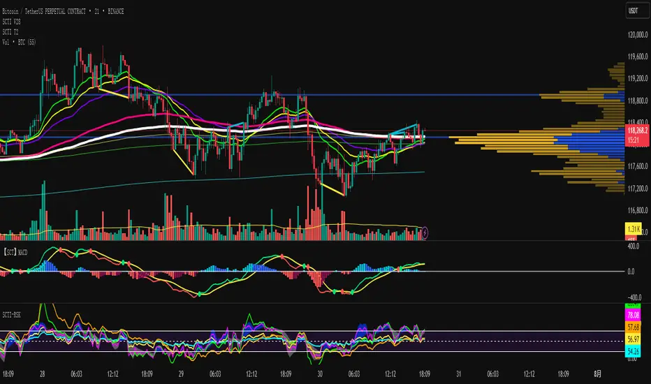
TrendTwisterV1.5 (Forex Ready + Indicators)A Precision Trend-Following TradingView Strategy for Forex**
HullShiftFX is a Pine Script strategy for TradingView that combines the power of the **Hull Moving Average (HMA)** and a **shifted Exponential Moving Average (EMA)** with multi-layered momentum filters including **RSI** and **dual Stochastic Oscillators**.
It’s designed for traders looking to catch high-probability breakouts with tight risk management and visual clarity.
Chart settings:
1. Select "Auto - Fits data to screen"
2. Please Select "Scale Price Chart Only" (To make the chart not squished)
### ✅ Entry Conditions
**Long Position:**
- Price closes above the 12-period Hull Moving Average.
- Price closes above the 5-period EMA shifted forward by 2 bars.
- RSI is above 50.
- Stochastic Oscillator (12,3,3) %K is above 50.
- Stochastic Oscillator (5,3,3) %K is above 50.
- Hull MA crosses above the shifted EMA.
**Short Position:**
- Price closes below the 12-period Hull Moving Average.
- Price closes below the 5-period EMA shifted forward by 2 bars.
- RSI is below 50.
- Stochastic Oscillator (12,3,3) %K is below 50.
- Stochastic Oscillator (5,3,3) %K is below 50.
- Hull MA crosses below the shifted EMA.
---
## 📉 Risk Management
- **Stop Loss:** Set at the low (for long) or high (for short) of the previous 2 candles.
- **Take Profit:** Calculated at a risk/reward ratio of **1.65x** the stop loss distance.
---
## 📊 Indicators Used
- **Hull Moving Average (12)**
- **Exponential Moving Average (5) **
- **Relative Strength Index (14)**
- **Stochastic Oscillators:**
- %K (12,3,3)
- %K (5,3,3)
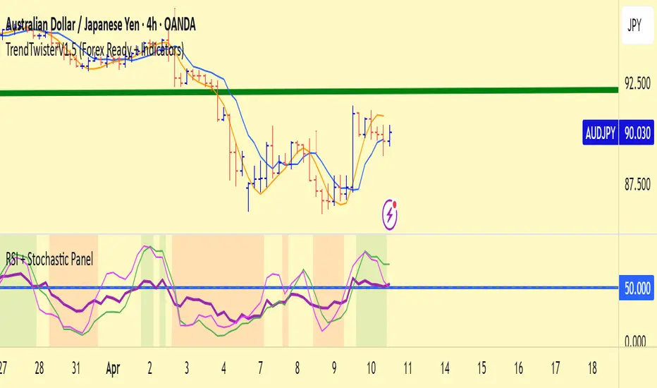
ZigZag█ Overview
This Pine Script™ library provides a comprehensive implementation of the ZigZag indicator using advanced object-oriented programming techniques. It serves as a developer resource rather than a standalone indicator, enabling Pine Script™ programmers to incorporate sophisticated ZigZag calculations into their own scripts.
Pine Script™ libraries contain reusable code that can be imported into indicators, strategies, and other libraries. For more information, consult the Libraries section of the Pine Script™ User Manual.
█ About the Original
This library is based on TradingView's official ZigZag implementation .
The original code provides a solid foundation with user-defined types and methods for calculating ZigZag pivot points.
█ What is ZigZag?
The ZigZag indicator filters out minor price movements to highlight significant market trends.
It works by:
1. Identifying significant pivot points (local highs and lows)
2. Connecting these points with straight lines
3. Ignoring smaller price movements that fall below a specified threshold
Traders typically use ZigZag for:
- Trend confirmation
- Identifying support and resistance levels
- Pattern recognition (such as Elliott Waves)
- Filtering out market noise
The algorithm identifies pivot points by analyzing price action over a specified number of bars, then only changes direction when price movement exceeds a user-defined percentage threshold.
█ My Enhancements
This modified version extends the original library with several key improvements:
1. Support and Resistance Visualization
- Adds horizontal lines at pivot points
- Customizable line length (offset from pivot)
- Adjustable line width and color
- Option to extend lines to the right edge of the chart
2. Support and Resistance Zones
- Creates semi-transparent zone areas around pivot points
- Customizable width for better visibility of important price levels
- Separate colors for support (lows) and resistance (highs)
- Visual representation of price areas rather than just single lines
3. Zig Zag Lines
- Separate colors for upward and downward ZigZag movements
- Visually distinguishes between bullish and bearish price swings
- Customizable colors for text
- Width customization
4. Enhanced Settings Structure
- Added new fields to the Settings type to support the additional features
- Extended Pivot type with supportResistance and supportResistanceZone fields
- Comprehensive configuration options for visual elements
These enhancements make the ZigZag more useful for technical analysis by clearly highlighting support/resistance levels and zones, and providing clearer visual cues about market direction.
█ Technical Implementation
This library leverages Pine Script™'s user-defined types (UDTs) to create a robust object-oriented architecture:
- Settings : Stores configuration parameters for calculation and display
- Pivot : Represents pivot points with their visual elements and properties
- ZigZag : Manages the overall state and behavior of the indicator
The implementation follows best practices from the Pine Script™ User Manual's Style Guide and uses advanced language features like methods and object references. These UDTs represent Pine Script™'s most advanced feature set, enabling sophisticated data structures and improved code organization.
For newcomers to Pine Script™, it's recommended to understand the language fundamentals before working with the UDT implementation in this library.
█ Usage Example
//@version=6
indicator("ZigZag Example", overlay = true, shorttitle = 'ZZA', max_bars_back = 5000, max_lines_count = 500, max_labels_count = 500, max_boxes_count = 500)
import andre_007/ZigZag/1 as ZIG
var group_1 = "ZigZag Settings"
//@variable Draw Zig Zag on the chart.
bool showZigZag = input.bool(true, "Show Zig-Zag Lines", group = group_1, tooltip = "If checked, the Zig Zag will be drawn on the chart.", inline = "1")
// @variable The deviation percentage from the last local high or low required to form a new Zig Zag point.
float deviationInput = input.float(5.0, "Deviation (%)", minval = 0.00001, maxval = 100.0,
tooltip = "The minimum percentage deviation from a previous pivot point required to change the Zig Zag's direction.", group = group_1, inline = "2")
// @variable The number of bars required for pivot detection.
int depthInput = input.int(10, "Depth", minval = 1, tooltip = "The number of bars required for pivot point detection.", group = group_1, inline = "3")
// @variable registerPivot (series bool) Optional. If `true`, the function compares a detected pivot
// point's coordinates to the latest `Pivot` object's `end` chart point, then
// updates the latest `Pivot` instance or adds a new instance to the `ZigZag`
// object's `pivots` array. If `false`, it does not modify the `ZigZag` object's
// data. The default is `true`.
bool allowZigZagOnOneBarInput = input.bool(true, "Allow Zig Zag on One Bar", tooltip = "If checked, the Zig Zag calculation can register a pivot high and pivot low on the same bar.",
group = group_1, inline = "allowZigZagOnOneBar")
var group_2 = "Display Settings"
// @variable The color of the Zig Zag's lines (up).
color lineColorUpInput = input.color(color.green, "Line Colors for Up/Down", group = group_2, inline = "4")
// @variable The color of the Zig Zag's lines (down).
color lineColorDownInput = input.color(color.red, "", group = group_2, inline = "4",
tooltip = "The color of the Zig Zag's lines")
// @variable The width of the Zig Zag's lines.
int lineWidthInput = input.int(1, "Line Width", minval = 1, tooltip = "The width of the Zig Zag's lines.", group = group_2, inline = "w")
// @variable If `true`, the Zig Zag will also display a line connecting the last known pivot to the current `close`.
bool extendInput = input.bool(true, "Extend to Last Bar", tooltip = "If checked, the last pivot will be connected to the current close.",
group = group_1, inline = "5")
// @variable If `true`, the pivot labels will display their price values.
bool showPriceInput = input.bool(true, "Display Reversal Price",
tooltip = "If checked, the pivot labels will display their price values.", group = group_2, inline = "6")
// @variable If `true`, each pivot label will display the volume accumulated since the previous pivot.
bool showVolInput = input.bool(true, "Display Cumulative Volume",
tooltip = "If checked, the pivot labels will display the volume accumulated since the previous pivot.", group = group_2, inline = "7")
// @variable If `true`, each pivot label will display the change in price from the previous pivot.
bool showChgInput = input.bool(true, "Display Reversal Price Change",
tooltip = "If checked, the pivot labels will display the change in price from the previous pivot.", group = group_2, inline = "8")
// @variable Controls whether the labels show price changes as raw values or percentages when `showChgInput` is `true`.
string priceDiffInput = input.string("Absolute", "", options = ,
tooltip = "Controls whether the labels show price changes as raw values or percentages when 'Display Reversal Price Change' is checked.",
group = group_2, inline = "8")
// @variable If `true`, the Zig Zag will display support and resistance lines.
bool showSupportResistanceInput = input.bool(true, "Show Support/Resistance Lines",
tooltip = "If checked, the Zig Zag will display support and resistance lines.", group = group_2, inline = "9")
// @variable The number of bars to extend the support and resistance lines from the last pivot point.
int supportResistanceOffsetInput = input.int(50, "Support/Resistance Offset", minval = 0,
tooltip = "The number of bars to extend the support and resistance lines from the last pivot point.", group = group_2, inline = "10")
// @variable The width of the support and resistance lines.
int supportResistanceWidthInput = input.int(1, "Support/Resistance Width", minval = 1,
tooltip = "The width of the support and resistance lines.", group = group_2, inline = "11")
// @variable The color of the support lines.
color supportColorInput = input.color(color.red, "Support/Resistance Color", group = group_2, inline = "12")
// @variable The color of the resistance lines.
color resistanceColorInput = input.color(color.green, "", group = group_2, inline = "12",
tooltip = "The color of the support/resistance lines.")
// @variable If `true`, the support and resistance lines will be drawn as zones.
bool showSupportResistanceZoneInput = input.bool(true, "Show Support/Resistance Zones",
tooltip = "If checked, the support and resistance lines will be drawn as zones.", group = group_2, inline = "12-1")
// @variable The color of the support zones.
color supportZoneColorInput = input.color(color.new(color.red, 70), "Support Zone Color", group = group_2, inline = "12-2")
// @variable The color of the resistance zones.
color resistanceZoneColorInput = input.color(color.new(color.green, 70), "", group = group_2, inline = "12-2",
tooltip = "The color of the support/resistance zones.")
// @variable The width of the support and resistance zones.
int supportResistanceZoneWidthInput = input.int(10, "Support/Resistance Zone Width", minval = 1,
tooltip = "The width of the support and resistance zones.", group = group_2, inline = "12-3")
// @variable If `true`, the support and resistance lines will extend to the right of the chart.
bool supportResistanceExtendInput = input.bool(false, "Extend to Right",
tooltip = "If checked, the lines will extend to the right of the chart.", group = group_2, inline = "13")
// @variable References a `Settings` instance that defines the `ZigZag` object's calculation and display properties.
var ZIG.Settings settings =
ZIG.Settings.new(
devThreshold = deviationInput,
depth = depthInput,
lineColorUp = lineColorUpInput,
lineColorDown = lineColorDownInput,
textUpColor = lineColorUpInput,
textDownColor = lineColorDownInput,
lineWidth = lineWidthInput,
extendLast = extendInput,
displayReversalPrice = showPriceInput,
displayCumulativeVolume = showVolInput,
displayReversalPriceChange = showChgInput,
differencePriceMode = priceDiffInput,
draw = showZigZag,
allowZigZagOnOneBar = allowZigZagOnOneBarInput,
drawSupportResistance = showSupportResistanceInput,
supportResistanceOffset = supportResistanceOffsetInput,
supportResistanceWidth = supportResistanceWidthInput,
supportColor = supportColorInput,
resistanceColor = resistanceColorInput,
supportResistanceExtend = supportResistanceExtendInput,
supportResistanceZoneWidth = supportResistanceZoneWidthInput,
drawSupportResistanceZone = showSupportResistanceZoneInput,
supportZoneColor = supportZoneColorInput,
resistanceZoneColor = resistanceZoneColorInput
)
// @variable References a `ZigZag` object created using the `settings`.
var ZIG.ZigZag zigZag = ZIG.newInstance(settings)
// Update the `zigZag` on every bar.
zigZag.update()
//#endregion
The example code demonstrates how to create a ZigZag indicator with customizable settings. It:
1. Creates a Settings object with user-defined parameters
2. Instantiates a ZigZag object using these settings
3. Updates the ZigZag on each bar to detect new pivot points
4. Automatically draws lines and labels when pivots are detected
This approach provides maximum flexibility while maintaining readability and ease of use.

ArbitrageDashboardv3310824This indicator allows you to monitor the spread (difference in exchange rates) between two assets in real-time for up to 12 trading pairs simultaneously.
⚙️ How does the indicator work?
In the settings menu, you can select two trading pairs, such as BTCUSDT on Binance and BTCUSDT on Bybit. The script then fetches prices from both exchanges and compares them, calculating the percentage difference (spread). This process is repeated for all 12 trading pairs added in the settings. The script works only with the assets and exchanges available on TradingView.
⚡️ How to use it?
When the spread is negative, it means the asset's price on the first exchange is lower than on the second. By buying on the first exchange and selling on the second, you can make a profit (taking into account the exchange fees). When the spread is positive, the opposite is true. The buy prices and exchanges are shown in a green Buy row, while sell prices and exchanges are displayed in a red Sell row. If the spread is zero, prices are the same on both exchanges, and no arbitrage opportunity exists. For better accuracy, use the smallest timeframe available in your TradingView subscription, such as minute or second intervals.
🕒 Arbitrage Situation Counter
For each trading pair, the table below the Buy row shows the number of arbitrage situations within a specified timeframe. An arbitrage situation occurs when the spread exceeds the Signal Threshold Level set by the user. Each time this happens, the counter increases by one. It only counts situations that occurred within the selected timeframe, such as the past hour for a 1-hour period. You can track arbitrage situations for up to three different periods simultaneously, ranging from 5 minutes to 24 hours. This counter helps evaluate the potential for arbitrage in the selected trading pairs. If a pair shows only 1-2 arbitrage situations per hour, it might be better to look for another pair.
🔔 Setting Up Alerts
In the script settings, you can set the Spread Signal Threshold. When the spread reaches this level, the table for that asset will be highlighted. This threshold also acts as a signal for setting up alerts. To set alerts, go to the Alerts tab in the TradingView menu on the right, click "Create Alert", and select this indicator under "Condition". You can then name the alert and finish the setup by clicking "Create".
We, the authors, have long been involved in cryptocurrency arbitrage and created this script for our own trading, but you can use it for any assets and markets as you see fit.
We also offer lighter versions of the indicator that track the spread for one or three trading pairs. These versions also display the spread chart, which can be useful for historical analysis. If the full indicator is too resource-intensive for your device, try these lighter versions:
🧩 Arbitrage Spread v1 : 1 pair + 1 chart
🧩 Arbitrage Spread v2 : 3 pairs + 3 charts
If your hardware can handle it, you can use the 12-pair version as a dashboard and add one of the versions with a spread chart for a detailed view of one or three pairs.
--
Этот индикатор позволяет в реальном времени отслеживать изменение спреда (разницы в цене) между двумя активами для 12 торговых пар одновременно.
⚙️ Как работает индикатор?
В меню настроек индикатора пользователь выбирает две торговые пары, например BTCUSDT на бирже Binance и BTCUSDT на бирже Bybit. Скрипт получает цены с обеих бирж и сравнивает их, рассчитывая процентное отклонение (спред). Этот процесс выполняется для всех 12 торговых пар, указанных в настройках. Скрипт работает только с теми активами и биржами, которые доступны на TradingView.
⚡️ Как использовать?
Когда спред отрицательный, это означает, что цена на первый актив ниже, чем на второй. В таком случае можно купить актив на первой бирже и продать на второй, получив прибыль (не забывая учитывать биржевые комиссии). Когда спред положительный, ситуация обратная. Биржи и цены для покупки отображаются в зеленой строке Buy, а для продажи – в красной строке Sell. При нулевом спреде цены на обеих биржах одинаковы, и арбитражная ситуация отсутствует.
Для повышения точности индикатора используйте минимально доступный таймфрейм на TradingView – минутный или секундный.
🕒 Счетчик арбитражных ситуаций
По каждой торговой паре в таблице под строкой Buy отображается количество арбитражных ситуаций за определенный промежуток времени. Арбитражная ситуация возникает, когда спред превышает установленный пользователем сигнальный уровень (Signal Threshold Level). При каждом превышении этого уровня счетчик увеличивается на единицу. Счетчик учитывает арбитражные ситуации за определенный период, например, за последний час для 1-часового периода (1h). Можно отслеживать количество арбитражных ситуаций одновременно для трех временных периодов от 5 минут до суток.
Счетчик помогает оценить перспективность арбитража выбранных пар. Если за час на паре было всего 1-2 арбитражные ситуации, возможно, лучше поискать другую пару.
🔔 Настройка оповещений
В настройках скрипта можно задать пороговое значение спреда (Spread Signal Threshold). Когда спред достигнет этого уровня, таблица для данного актива будет подсвечена. Этот уровень также служит сигналом для настройки оповещений.
Для настройки оповещений откройте вкладку «Оповещения» в меню TradingView справа. Нажмите кнопку «Создать оповещение». В открывшемся окне в строке «Условие» выберите данный индикатор. Затем задайте название и завершите настройку, нажав кнопку «Создать».
Мы, авторы этого скрипта, давно занимаемся арбитражем криптовалют и создали его для себя, но вы можете использовать его для любых активов и на любых рынках по своему усмотрению.
У нас также есть более простая версия индикатора, которая отслеживает спред для одной или трех торговых пар. В этих версиях можно просматривать график самого спреда, что полезно для оценки его динамики. Если этот индикатор кажется вам или вашему устройству слишком тяжелым, вы можете воспользоваться облегченными версиями:
🧩 Arbitrage Spread v1 : 1 пара + 1 график
🧩 Arbitrage Spread v2 : 3 пары + 3 графика
Если ваше оборудование позволяет, вы можете добавить несколько индикаторов на экран. Например, использовать версию с 12 парами как дашборд, а одну из версий с графиком спреда для более детального анализа по одному или трем инструментам.
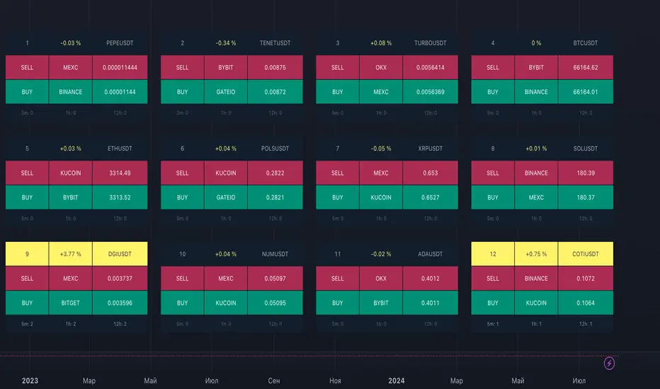
PubLibTrendLibrary "PubLibTrend"
trend, multi-part trend, double trend and multi-part double trend conditions for indicator and strategy development
rlut()
return line uptrend condition
Returns: bool
dt()
downtrend condition
Returns: bool
ut()
uptrend condition
Returns: bool
rldt()
return line downtrend condition
Returns: bool
dtop()
double top condition
Returns: bool
dbot()
double bottom condition
Returns: bool
rlut_1p()
1-part return line uptrend condition
Returns: bool
rlut_2p()
2-part return line uptrend condition
Returns: bool
rlut_3p()
3-part return line uptrend condition
Returns: bool
rlut_4p()
4-part return line uptrend condition
Returns: bool
rlut_5p()
5-part return line uptrend condition
Returns: bool
rlut_6p()
6-part return line uptrend condition
Returns: bool
rlut_7p()
7-part return line uptrend condition
Returns: bool
rlut_8p()
8-part return line uptrend condition
Returns: bool
rlut_9p()
9-part return line uptrend condition
Returns: bool
rlut_10p()
10-part return line uptrend condition
Returns: bool
rlut_11p()
11-part return line uptrend condition
Returns: bool
rlut_12p()
12-part return line uptrend condition
Returns: bool
rlut_13p()
13-part return line uptrend condition
Returns: bool
rlut_14p()
14-part return line uptrend condition
Returns: bool
rlut_15p()
15-part return line uptrend condition
Returns: bool
rlut_16p()
16-part return line uptrend condition
Returns: bool
rlut_17p()
17-part return line uptrend condition
Returns: bool
rlut_18p()
18-part return line uptrend condition
Returns: bool
rlut_19p()
19-part return line uptrend condition
Returns: bool
rlut_20p()
20-part return line uptrend condition
Returns: bool
rlut_21p()
21-part return line uptrend condition
Returns: bool
rlut_22p()
22-part return line uptrend condition
Returns: bool
rlut_23p()
23-part return line uptrend condition
Returns: bool
rlut_24p()
24-part return line uptrend condition
Returns: bool
rlut_25p()
25-part return line uptrend condition
Returns: bool
rlut_26p()
26-part return line uptrend condition
Returns: bool
rlut_27p()
27-part return line uptrend condition
Returns: bool
rlut_28p()
28-part return line uptrend condition
Returns: bool
rlut_29p()
29-part return line uptrend condition
Returns: bool
rlut_30p()
30-part return line uptrend condition
Returns: bool
dt_1p()
1-part downtrend condition
Returns: bool
dt_2p()
2-part downtrend condition
Returns: bool
dt_3p()
3-part downtrend condition
Returns: bool
dt_4p()
4-part downtrend condition
Returns: bool
dt_5p()
5-part downtrend condition
Returns: bool
dt_6p()
6-part downtrend condition
Returns: bool
dt_7p()
7-part downtrend condition
Returns: bool
dt_8p()
8-part downtrend condition
Returns: bool
dt_9p()
9-part downtrend condition
Returns: bool
dt_10p()
10-part downtrend condition
Returns: bool
dt_11p()
11-part downtrend condition
Returns: bool
dt_12p()
12-part downtrend condition
Returns: bool
dt_13p()
13-part downtrend condition
Returns: bool
dt_14p()
14-part downtrend condition
Returns: bool
dt_15p()
15-part downtrend condition
Returns: bool
dt_16p()
16-part downtrend condition
Returns: bool
dt_17p()
17-part downtrend condition
Returns: bool
dt_18p()
18-part downtrend condition
Returns: bool
dt_19p()
19-part downtrend condition
Returns: bool
dt_20p()
20-part downtrend condition
Returns: bool
dt_21p()
21-part downtrend condition
Returns: bool
dt_22p()
22-part downtrend condition
Returns: bool
dt_23p()
23-part downtrend condition
Returns: bool
dt_24p()
24-part downtrend condition
Returns: bool
dt_25p()
25-part downtrend condition
Returns: bool
dt_26p()
26-part downtrend condition
Returns: bool
dt_27p()
27-part downtrend condition
Returns: bool
dt_28p()
28-part downtrend condition
Returns: bool
dt_29p()
29-part downtrend condition
Returns: bool
dt_30p()
30-part downtrend condition
Returns: bool
ut_1p()
1-part uptrend condition
Returns: bool
ut_2p()
2-part uptrend condition
Returns: bool
ut_3p()
3-part uptrend condition
Returns: bool
ut_4p()
4-part uptrend condition
Returns: bool
ut_5p()
5-part uptrend condition
Returns: bool
ut_6p()
6-part uptrend condition
Returns: bool
ut_7p()
7-part uptrend condition
Returns: bool
ut_8p()
8-part uptrend condition
Returns: bool
ut_9p()
9-part uptrend condition
Returns: bool
ut_10p()
10-part uptrend condition
Returns: bool
ut_11p()
11-part uptrend condition
Returns: bool
ut_12p()
12-part uptrend condition
Returns: bool
ut_13p()
13-part uptrend condition
Returns: bool
ut_14p()
14-part uptrend condition
Returns: bool
ut_15p()
15-part uptrend condition
Returns: bool
ut_16p()
16-part uptrend condition
Returns: bool
ut_17p()
17-part uptrend condition
Returns: bool
ut_18p()
18-part uptrend condition
Returns: bool
ut_19p()
19-part uptrend condition
Returns: bool
ut_20p()
20-part uptrend condition
Returns: bool
ut_21p()
21-part uptrend condition
Returns: bool
ut_22p()
22-part uptrend condition
Returns: bool
ut_23p()
23-part uptrend condition
Returns: bool
ut_24p()
24-part uptrend condition
Returns: bool
ut_25p()
25-part uptrend condition
Returns: bool
ut_26p()
26-part uptrend condition
Returns: bool
ut_27p()
27-part uptrend condition
Returns: bool
ut_28p()
28-part uptrend condition
Returns: bool
ut_29p()
29-part uptrend condition
Returns: bool
ut_30p()
30-part uptrend condition
Returns: bool
rldt_1p()
1-part return line downtrend condition
Returns: bool
rldt_2p()
2-part return line downtrend condition
Returns: bool
rldt_3p()
3-part return line downtrend condition
Returns: bool
rldt_4p()
4-part return line downtrend condition
Returns: bool
rldt_5p()
5-part return line downtrend condition
Returns: bool
rldt_6p()
6-part return line downtrend condition
Returns: bool
rldt_7p()
7-part return line downtrend condition
Returns: bool
rldt_8p()
8-part return line downtrend condition
Returns: bool
rldt_9p()
9-part return line downtrend condition
Returns: bool
rldt_10p()
10-part return line downtrend condition
Returns: bool
rldt_11p()
11-part return line downtrend condition
Returns: bool
rldt_12p()
12-part return line downtrend condition
Returns: bool
rldt_13p()
13-part return line downtrend condition
Returns: bool
rldt_14p()
14-part return line downtrend condition
Returns: bool
rldt_15p()
15-part return line downtrend condition
Returns: bool
rldt_16p()
16-part return line downtrend condition
Returns: bool
rldt_17p()
17-part return line downtrend condition
Returns: bool
rldt_18p()
18-part return line downtrend condition
Returns: bool
rldt_19p()
19-part return line downtrend condition
Returns: bool
rldt_20p()
20-part return line downtrend condition
Returns: bool
rldt_21p()
21-part return line downtrend condition
Returns: bool
rldt_22p()
22-part return line downtrend condition
Returns: bool
rldt_23p()
23-part return line downtrend condition
Returns: bool
rldt_24p()
24-part return line downtrend condition
Returns: bool
rldt_25p()
25-part return line downtrend condition
Returns: bool
rldt_26p()
26-part return line downtrend condition
Returns: bool
rldt_27p()
27-part return line downtrend condition
Returns: bool
rldt_28p()
28-part return line downtrend condition
Returns: bool
rldt_29p()
29-part return line downtrend condition
Returns: bool
rldt_30p()
30-part return line downtrend condition
Returns: bool
dut()
double uptrend condition
Returns: bool
ddt()
double downtrend condition
Returns: bool
dut_1p()
1-part double uptrend condition
Returns: bool
dut_2p()
2-part double uptrend condition
Returns: bool
dut_3p()
3-part double uptrend condition
Returns: bool
dut_4p()
4-part double uptrend condition
Returns: bool
dut_5p()
5-part double uptrend condition
Returns: bool
dut_6p()
6-part double uptrend condition
Returns: bool
dut_7p()
7-part double uptrend condition
Returns: bool
dut_8p()
8-part double uptrend condition
Returns: bool
dut_9p()
9-part double uptrend condition
Returns: bool
dut_10p()
10-part double uptrend condition
Returns: bool
dut_11p()
11-part double uptrend condition
Returns: bool
dut_12p()
12-part double uptrend condition
Returns: bool
dut_13p()
13-part double uptrend condition
Returns: bool
dut_14p()
14-part double uptrend condition
Returns: bool
dut_15p()
15-part double uptrend condition
Returns: bool
dut_16p()
16-part double uptrend condition
Returns: bool
dut_17p()
17-part double uptrend condition
Returns: bool
dut_18p()
18-part double uptrend condition
Returns: bool
dut_19p()
19-part double uptrend condition
Returns: bool
dut_20p()
20-part double uptrend condition
Returns: bool
dut_21p()
21-part double uptrend condition
Returns: bool
dut_22p()
22-part double uptrend condition
Returns: bool
dut_23p()
23-part double uptrend condition
Returns: bool
dut_24p()
24-part double uptrend condition
Returns: bool
dut_25p()
25-part double uptrend condition
Returns: bool
dut_26p()
26-part double uptrend condition
Returns: bool
dut_27p()
27-part double uptrend condition
Returns: bool
dut_28p()
28-part double uptrend condition
Returns: bool
dut_29p()
29-part double uptrend condition
Returns: bool
dut_30p()
30-part double uptrend condition
Returns: bool
ddt_1p()
1-part double downtrend condition
Returns: bool
ddt_2p()
2-part double downtrend condition
Returns: bool
ddt_3p()
3-part double downtrend condition
Returns: bool
ddt_4p()
4-part double downtrend condition
Returns: bool
ddt_5p()
5-part double downtrend condition
Returns: bool
ddt_6p()
6-part double downtrend condition
Returns: bool
ddt_7p()
7-part double downtrend condition
Returns: bool
ddt_8p()
8-part double downtrend condition
Returns: bool
ddt_9p()
9-part double downtrend condition
Returns: bool
ddt_10p()
10-part double downtrend condition
Returns: bool
ddt_11p()
11-part double downtrend condition
Returns: bool
ddt_12p()
12-part double downtrend condition
Returns: bool
ddt_13p()
13-part double downtrend condition
Returns: bool
ddt_14p()
14-part double downtrend condition
Returns: bool
ddt_15p()
15-part double downtrend condition
Returns: bool
ddt_16p()
16-part double downtrend condition
Returns: bool
ddt_17p()
17-part double downtrend condition
Returns: bool
ddt_18p()
18-part double downtrend condition
Returns: bool
ddt_19p()
19-part double downtrend condition
Returns: bool
ddt_20p()
20-part double downtrend condition
Returns: bool
ddt_21p()
21-part double downtrend condition
Returns: bool
ddt_22p()
22-part double downtrend condition
Returns: bool
ddt_23p()
23-part double downtrend condition
Returns: bool
ddt_24p()
24-part double downtrend condition
Returns: bool
ddt_25p()
25-part double downtrend condition
Returns: bool
ddt_26p()
26-part double downtrend condition
Returns: bool
ddt_27p()
27-part double downtrend condition
Returns: bool
ddt_28p()
28-part double downtrend condition
Returns: bool
ddt_29p()
29-part double downtrend condition
Returns: bool
ddt_30p()
30-part double downtrend condition
Returns: bool

Rise Sense Capital - RSI MACD Spot Buying IndicatorToday, I'll share a spot buying strategy shared by a member @KR陳 within the DATA Trader Alliance Alpha group. First, you need to prepare two indicators:
今天分享一個DATA交易者聯盟Alpha群組裏面的群友@KR陳分享的現貨買入策略。
首先需要準備兩個指標
RSI Indicator (Relative Strength Index) - RSI is a technical analysis tool based on price movements over a period of time to evaluate the speed and magnitude of price changes. RSI calculates the changes in price over a period to determine whether the recent trend is relatively strong (bullish) or weak (bearish).
RSI指標,(英文全名:Relative Strength Index),中文稱為「相對強弱指標」,是一種以股價漲跌為基礎,在一段時間內的收盤價,用於評估價格變動的速度 (快慢) 與變化 (幅度) 的技術分析工具,RSI藉由計算一段期間內股價的漲跌變化,判斷最近的趨勢屬於偏強 (偏多) 還是偏弱 (偏空)。
MACD Indicator (Moving Average Convergence & Divergence) - MACD is a technical analysis tool proposed by Gerald Appel in the 1970s. It is commonly used in trading to determine trend reversals by analyzing the convergence and divergence of fast and slow lines.
MACD 指標 (Moving Average Convergence & Divergence) 中文名為平滑異同移動平均線指標,MACD 是在 1970 年代由美國人 Gerald Appel 所提出,是一項歷史悠久且經常在交易中被使用的技術分析工具,原理是利用快慢線的交錯,藉以判斷股價走勢的轉折。
In MACD analysis, the most commonly used values are 12, 26, and 9, known as MACD (12,26,9). The market often uses the MACD indicator to determine the future direction of assets and to identify entry and exit points.
在 MACD 的技術分析中,最常用的值為 12 天、26 天、9 天,也稱為 MACD (12,26,9),市場常用 MACD 指標來判斷操作標的的後市走向,確定波段漲幅並找到進、出場點。
Strategy analysis by member KR陳:
策略解析 by群友 KR陳 :
Condition 1: RSI value in the previous candle is below oversold zone(30).
條件1:RSI 在前一根的數值低於超賣區(30)
buycondition1 = RSI <30
Condition 2: MACD histogram changes from decreasing to increasing.
條件2:MACD柱由遞減轉遞增
buycondition2 = hist >hist and hist
Absolute Momentum (Time Series Momentum)Absolute momentum , also known as time series momentum , focuses on the trend of an asset's own past performance to predict its future performance. It involves analyzing an asset's own historical performance, rather than comparing it to other assets.
The strategy determines whether an asset's price is exhibiting an upward (positive momentum) or downward (negative momentum) trend by assessing the asset's return over a given period (standard look-back period: 12 months or approximately 250 trading days). Some studies recommend calculating momentum by deducting the corresponding Treasury bill rate from the measured performance.
Absolute Momentum Indicator
The Absolute Momentum Indicator displays the rolling 12-month performance (measured over 250 trading days) and plots it against a horizontal line representing 0%. If the indicator crosses above this line, it signifies positive absolute momentum, and conversely, crossing below indicates negative momentum. An additional, optional look-back period input field can be accessed through the settings.
Hint: This indicator is a simplified version, as some academic approaches measure absolute momentum by subtracting risk-free rates from the 12-month performance. However, even with higher rates, the values will still remain close to the 0% line.
Benefits of Absolute Momentum
Absolute momentum, which should not be confused with relative momentum or the momentum indicator, serves as a timing instrument for both individual assets and entire markets.
Gary Antonacci , a key contributor to the absolute momentum strategy (find study below), emphasizes its effectiveness in multi-asset portfolios and its importance in long-only investing. This is particularly evident in a) reducing downside volatility and b) mitigating behavioral biases.
Moskowitz, Ooi, and Pedersen document significant 'time series momentum' across various asset classes, including equity index, currency, commodity, and bond futures, in 58 liquid instruments (find study below). There's a notable persistence in returns ranging from one to 12 months, which tends to partially reverse over longer periods. This pattern aligns with sentiment theories suggesting initial under-reaction followed by delayed over-reaction.
Despite its surprising ease of implementation, the academic community has successfully measured the effects of absolute momentum across decades and in every major asset class, including stocks, bonds, commodities, and foreign exchange (FX).
Strategies for Implementing Absolute Momentum:
To Buy a Stock:
Select a Look-Back Period: Choose a historical period to analyze the stock's performance. A common period is 12 months, but this can vary based on your investment strategy.
Calculate Excess Return: Determine the stock's excess return over this period. You can also assume a risk-free rate of "0" to simplify the process.
Evaluate Momentum:
If the excess return is positive, it indicates positive absolute momentum. This suggests the stock is in an upward trend and could be a good buying opportunity.
If the excess return is negative, it suggests negative momentum, and you might want to delay buying.
Consider further conditions: Align your decision with broader market trends, economic indicators, or fundamental analysis, for additional context.
To Sell a Stock You Own:
Regularly Monitor Performance: Use the same look-back period as for buying (e.g., 12 months) to regularly assess the stock's performance.
Check for Negative Momentum: Calculate the excess return for the look-back period. Again, you can assume a risk-free rate of "0" to simplify the process. If the stock shows negative momentum, it might be time to consider selling.
Consider further conditions:Align your decision with broader market trends, economic indicators, or fundamental analysis, for additional context.
Important note: Note: Entering a position (i.e., buying) based on positive absolute momentum doesn't necessarily mean you must sell it if it later exhibits negative absolute momentum. You can initiate a position using positive absolute momentum as an entry indicator and then continue holding it based on other criteria, such as fundamental analysis.
General Tips:
Reassessment Frequency: Decide how often you will reassess the momentum (monthly, quarterly, etc.).
Remember, while absolute momentum provides a systematic approach, it's recommendable to consider it as part of a broader investment strategy that includes diversification, risk management, fundamental analysis, etc.
Relevant Capital Market Studies:
Antonacci, Gary. "Absolute momentum: A simple rule-based strategy and universal trend-following overlay." Available at SSRN 2244633 (2013)
Moskowitz, Tobias J., Yao Hua Ooi, and Lasse Heje Pedersen. "Time series momentum." Journal of financial economics 104.2 (2012): 228-250
S&P 500 Quandl Data & RatiosTradingView has a little-known integration that allows you to pull in 3rd party data-sets from Nasdaq Data Link, also known as Quandl. Today, I am open-sourcing for the community an indicator that uses the Quandl integration to pull in historical data and ratios on the S&P500. I originally coded this to study macro P/E ratios during peaks and troughs of boom/bust cycles.
The indicator pulls in each of the following datasets, as defined and provided by Quandl. The user can select which datasets to pull in using the indicator settings:
Dividend Yield : S&P 500 dividend yield (12 month dividend per share)/price. Yields following June 2022 (including the current yield) are estimated based on 12 month dividends through June 2022, as reported by S&P. Sources: Standard & Poor's for current S&P 500 Dividend Yield. Robert Shiller and his book Irrational Exuberance for historic S&P 500 Dividend Yields.
Price Earning Ratio : Price to earnings ratio, based on trailing twelve month as reported earnings. Current PE is estimated from latest reported earnings and current market price. Source: Robert Shiller and his book Irrational Exuberance for historic S&P 500 PE Ratio.
CAPE/Shiller PE Ratio : Shiller PE ratio for the S&P 500. Price earnings ratio is based on average inflation-adjusted earnings from the previous 10 years, known as the Cyclically Adjusted PE Ratio (CAPE Ratio), Shiller PE Ratio, or PE 10 FAQ. Data courtesy of Robert Shiller from his book, Irrational Exuberance.
Earnings Yield : S&P 500 Earnings Yield. Earnings Yield = trailing 12 month earnings divided by index price (or inverse PE) Yields following March, 2022 (including current yield) are estimated based on 12 month earnings through March, 2022 the latest reported by S&P. Source: Standard & Poor's
Price Book Ratio : S&P 500 price to book value ratio. Current price to book ratio is estimated based on current market price and S&P 500 book value as of March, 2022 the latest reported by S&P. Source: Standard & Poor's
Price Sales Ratio : S&P 500 Price to Sales Ratio (P/S or Price to Revenue). Current price to sales ratio is estimated based on current market price and 12 month sales ending March, 2022 the latest reported by S&P. Source: Standard & Poor's
Inflation Adjusted SP500 : Inflation adjusted SP500. Other than the current price, all prices are monthly average closing prices. Sources: Standard & Poor's Robert Shiller and his book Irrational Exuberance for historic S&P 500 prices, and historic CPIs.
Revenue Per Share : Trailing twelve month S&P 500 Sales Per Share (S&P 500 Revenue Per Share) non-inflation adjusted current dollars. Source: Standard & Poor's
Earnings Per Share : S&P 500 Earnings Per Share. 12-month real earnings per share inflation adjusted, constant August, 2022 dollars. Sources: Standard & Poor's for current S&P 500 Earnings. Robert Shiller and his book Irrational Exuberance for historic S&P 500 Earnings.
Disclaimer: This is not financial advice. Open-source scripts I publish in the community are largely meant to spark ideas that can be used as building blocks for part of a more robust trade management strategy. If you would like to implement a version of any script, I would recommend making significant additions/modifications to the strategy & risk management functions. If you don’t know how to program in Pine, then hire a Pine-coder. We can help!

Argo II - (alerts for 3commas composite bots) - publicThis script lets users create BUY/SELL alerts for 3commas composite bots (1 alert = 12 pairs) in a simple way, based on a built in set of indicators that can be tweaked to work together or alone through the study settings.
There is a version of this script for single pair bots, with slightly more features here .
If the user choses to create both BUY and SELL signals from the study settings, the (1) alert created will send both BUY and SELL signals for all 12 pairs selected. At this stage, the script forces the user to select 12 pairs in the study settings. If less pairs are inserted, it will not work. Also, the script will only send alerts for the pairs selected in the study settings, not for the current chart (if different).
How to use:
- Add the script to the current chart
- Open the study settings , insert bot details and select 12 pairs. You should write the pairs manually, using the format BTC , ADA, ETH, etc. They MUST be in capital letters or 3commas will not recognize them.
- Still in the study settings, tweak the deal start/close conditions from various indicators until happy. The study will plot the entry / exit points below the current chart (1 = buy, 2 = sell)
- Make sure your strategy works for all the pairs you have selected, simply by checking each chart with the same study settings
- When happy, right click on the "..." next to the study name, then "Add alert'".
- Under "Condition", on the second line, chose "Any alert () function call". Add the webhook from 3commas, give it a name, and "create".
That's it.
Notes:
- If you insert coins that are not available for the quote currency and exchange of your choosing, the script will not work and return an error.
- Make sure you run tests with paper trading or dummy bots (i.e without actual bot ID) to ensure your alerts trigger as intended on all coins.
- If alerts trigger too much (i.e they all trigger at the same time for all coins), Trading View will stop the alert. So probably not ideal for a scalping bot. It could also be the sign the script doesn't work as intended.
- The script is a bit slow on my side. I am a beginner in pinescript, so if anyone knows how to simplify it, please let me know.
- if anyone knows how to tell the script to function with less than 12 pairs (when not filling the 12 fields in the setting), please also let me know :)
XPloRR MA-Buy ATR-Trailing-Stop Long Term Strategy Beating B&HXPloRR MA-Buy ATR-MA-Trailing-Stop Strategy
Long term MA Trailing Stop strategy to beat Buy&Hold strategy
None of the strategies that I tested can beat the long term Buy&Hold strategy. That's the reason why I wrote this strategy.
Purpose: beat Buy&Hold strategy with around 10 trades. 100% capitalize sold trade into new trade.
My buy strategy is triggered by the EMA(blue) crossing over the SMA curve(orange).
My sell strategy is triggered by another EMA(lime) of the close value crossing the trailing stop(green) value.
The trailing stop value(green) is set to a multiple of the ATR(15) value.
ATR(15) is the SMA(15) value of the difference between high and low values.
Every stock has it's own "DNA", so first thing to do is find the right parameters to get the best strategy values voor EMA, SMA and Trailing Stop.
Then keep using these parameter for future buy/sell signals only for that particular stock.
Do the same for other stocks.
Here are the parameters:
Exponential MA: buy trigger when crossing over the SMA value (use values between 11-50)
Simple MA: buy trigger when EMA crosses over the SMA value (use values between 20 and 200)
Stop EMA: sell trigger when Stop EMA of close value crosses under the trailing stop value (use values between 8 and 16)
Trailing Stop #ATR: defines the trailing stop value as a multiple of the ATR(15) value
Example parameters for different stocks (Start capital: 1000, Order=100% of equity, Period 1/1/2005 to now):
BAR(Barco): EMA=11, SMA=82, StopEMA=12, Stop#ATR=9
Buy&HoldProfit: 45.82%, NetProfit: 294.7%, #Trades:8, %Profit:62.5%, ProfitFactor: 12.539
AAPL(Apple): EMA=12, SMA=45, StopEMA=12, Stop#ATR=6
Buy&HoldProfit: 2925.86%, NetProfit: 4035.92%, #Trades:10, %Profit:60%, ProfitFactor: 6.36
BEKB(Bekaert): EMA=12, SMA=42, StopEMA=12, Stop#ATR=7
Buy&HoldProfit: 81.11%, NetProfit: 521.37%, #Trades:10, %Profit:60%, ProfitFactor: 2.617
SOLB(Solvay): EMA=12, SMA=63, StopEMA=11, Stop#ATR=8
Buy&HoldProfit: 43.61%, NetProfit: 151.4%, #Trades:8, %Profit:75%, ProfitFactor: 3.794
PHIA(Philips): EMA=11, SMA=80, StopEMA=8, Stop#ATR=10
Buy&HoldProfit: 56.79%, NetProfit: 198.46%, #Trades:6, %Profit:83.33%, ProfitFactor: 23.07
I am very curious to see the parameters for your stocks and please make suggestions to improve this strategy.

Quantum Rotational Field MappingQuantum Rotational Field Mapping (QRFM):
Phase Coherence Detection Through Complex-Plane Oscillator Analysis
Quantum Rotational Field Mapping applies complex-plane mathematics and phase-space analysis to oscillator ensembles, identifying high-probability trend ignition points by measuring when multiple independent oscillators achieve phase coherence. Unlike traditional multi-oscillator approaches that simply stack indicators or use boolean AND/OR logic, this system converts each oscillator into a rotating phasor (vector) in the complex plane and calculates the Coherence Index (CI) —a mathematical measure of how tightly aligned the ensemble has become—then generates signals only when alignment, phase direction, and pairwise entanglement all converge.
The indicator combines three mathematical frameworks: phasor representation using analytic signal theory to extract phase and amplitude from each oscillator, coherence measurement using vector summation in the complex plane to quantify group alignment, and entanglement analysis that calculates pairwise phase agreement across all oscillator combinations. This creates a multi-dimensional confirmation system that distinguishes between random oscillator noise and genuine regime transitions.
What Makes This Original
Complex-Plane Phasor Framework
This indicator implements classical signal processing mathematics adapted for market oscillators. Each oscillator—whether RSI, MACD, Stochastic, CCI, Williams %R, MFI, ROC, or TSI—is first normalized to a common scale, then converted into a complex-plane representation using an in-phase (I) and quadrature (Q) component. The in-phase component is the oscillator value itself, while the quadrature component is calculated as the first difference (derivative proxy), creating a velocity-aware representation.
From these components, the system extracts:
Phase (φ) : Calculated as φ = atan2(Q, I), representing the oscillator's position in its cycle (mapped to -180° to +180°)
Amplitude (A) : Calculated as A = √(I² + Q²), representing the oscillator's strength or conviction
This mathematical approach is fundamentally different from simply reading oscillator values. A phasor captures both where an oscillator is in its cycle (phase angle) and how strongly it's expressing that position (amplitude). Two oscillators can have the same value but be in opposite phases of their cycles—traditional analysis would see them as identical, while QRFM sees them as 180° out of phase (contradictory).
Coherence Index Calculation
The core innovation is the Coherence Index (CI) , borrowed from physics and signal processing. When you have N oscillators, each with phase φₙ, you can represent each as a unit vector in the complex plane: e^(iφₙ) = cos(φₙ) + i·sin(φₙ).
The CI measures what happens when you sum all these vectors:
Resultant Vector : R = Σ e^(iφₙ) = Σ cos(φₙ) + i·Σ sin(φₙ)
Coherence Index : CI = |R| / N
Where |R| is the magnitude of the resultant vector and N is the number of active oscillators.
The CI ranges from 0 to 1:
CI = 1.0 : Perfect coherence—all oscillators have identical phase angles, vectors point in the same direction, creating maximum constructive interference
CI = 0.0 : Complete decoherence—oscillators are randomly distributed around the circle, vectors cancel out through destructive interference
0 < CI < 1 : Partial alignment—some clustering with some scatter
This is not a simple average or correlation. The CI captures phase synchronization across the entire ensemble simultaneously. When oscillators phase-lock (align their cycles), the CI spikes regardless of their individual values. This makes it sensitive to regime transitions that traditional indicators miss.
Dominant Phase and Direction Detection
Beyond measuring alignment strength, the system calculates the dominant phase of the ensemble—the direction the resultant vector points:
Dominant Phase : φ_dom = atan2(Σ sin(φₙ), Σ cos(φₙ))
This gives the "average direction" of all oscillator phases, mapped to -180° to +180°:
+90° to -90° (right half-plane): Bullish phase dominance
+90° to +180° or -90° to -180° (left half-plane): Bearish phase dominance
The combination of CI magnitude (coherence strength) and dominant phase angle (directional bias) creates a two-dimensional signal space. High CI alone is insufficient—you need high CI plus dominant phase pointing in a tradeable direction. This dual requirement is what separates QRFM from simple oscillator averaging.
Entanglement Matrix and Pairwise Coherence
While the CI measures global alignment, the entanglement matrix measures local pairwise relationships. For every pair of oscillators (i, j), the system calculates:
E(i,j) = |cos(φᵢ - φⱼ)|
This represents the phase agreement between oscillators i and j:
E = 1.0 : Oscillators are in-phase (0° or 360° apart)
E = 0.0 : Oscillators are in quadrature (90° apart, orthogonal)
E between 0 and 1 : Varying degrees of alignment
The system counts how many oscillator pairs exceed a user-defined entanglement threshold (e.g., 0.7). This entangled pairs count serves as a confirmation filter: signals require not just high global CI, but also a minimum number of strong pairwise agreements. This prevents false ignitions where CI is high but driven by only two oscillators while the rest remain scattered.
The entanglement matrix creates an N×N symmetric matrix that can be visualized as a web—when many cells are bright (high E values), the ensemble is highly interconnected. When cells are dark, oscillators are moving independently.
Phase-Lock Tolerance Mechanism
A complementary confirmation layer is the phase-lock detector . This calculates the maximum phase spread across all oscillators:
For all pairs (i,j), compute angular distance: Δφ = |φᵢ - φⱼ|, wrapping at 180°
Max Spread = maximum Δφ across all pairs
If max spread < user threshold (e.g., 35°), the ensemble is considered phase-locked —all oscillators are within a narrow angular band.
This differs from entanglement: entanglement measures pairwise cosine similarity (magnitude of alignment), while phase-lock measures maximum angular deviation (tightness of clustering). Both must be satisfied for the highest-conviction signals.
Multi-Layer Visual Architecture
QRFM includes six visual components that represent the same underlying mathematics from different perspectives:
Circular Orbit Plot : A polar coordinate grid showing each oscillator as a vector from origin to perimeter. Angle = phase, radius = amplitude. This is a real-time snapshot of the complex plane. When vectors converge (point in similar directions), coherence is high. When scattered randomly, coherence is low. Users can see phase alignment forming before CI numerically confirms it.
Phase-Time Heat Map : A 2D matrix with rows = oscillators and columns = time bins. Each cell is colored by the oscillator's phase at that time (using a gradient where color hue maps to angle). Horizontal color bands indicate sustained phase alignment over time. Vertical color bands show moments when all oscillators shared the same phase (ignition points). This provides historical pattern recognition.
Entanglement Web Matrix : An N×N grid showing E(i,j) for all pairs. Cells are colored by entanglement strength—bright yellow/gold for high E, dark gray for low E. This reveals which oscillators are driving coherence and which are lagging. For example, if RSI and MACD show high E but Stochastic shows low E with everything, Stochastic is the outlier.
Quantum Field Cloud : A background color overlay on the price chart. Color (green = bullish, red = bearish) is determined by dominant phase. Opacity is determined by CI—high CI creates dense, opaque cloud; low CI creates faint, nearly invisible cloud. This gives an atmospheric "feel" for regime strength without looking at numbers.
Phase Spiral : A smoothed plot of dominant phase over recent history, displayed as a curve that wraps around price. When the spiral is tight and rotating steadily, the ensemble is in coherent rotation (trending). When the spiral is loose or erratic, coherence is breaking down.
Dashboard : A table showing real-time metrics: CI (as percentage), dominant phase (in degrees with directional arrow), field strength (CI × average amplitude), entangled pairs count, phase-lock status (locked/unlocked), quantum state classification ("Ignition", "Coherent", "Collapse", "Chaos"), and collapse risk (recent CI change normalized to 0-100%).
Each component is independently toggleable, allowing users to customize their workspace. The orbit plot is the most essential—it provides intuitive, visual feedback on phase alignment that no numerical dashboard can match.
Core Components and How They Work Together
1. Oscillator Normalization Engine
The foundation is creating a common measurement scale. QRFM supports eight oscillators:
RSI : Normalized from to using overbought/oversold levels (70, 30) as anchors
MACD Histogram : Normalized by dividing by rolling standard deviation, then clamped to
Stochastic %K : Normalized from using (80, 20) anchors
CCI : Divided by 200 (typical extreme level), clamped to
Williams %R : Normalized from using (-20, -80) anchors
MFI : Normalized from using (80, 20) anchors
ROC : Divided by 10, clamped to
TSI : Divided by 50, clamped to
Each oscillator can be individually enabled/disabled. Only active oscillators contribute to phase calculations. The normalization removes scale differences—a reading of +0.8 means "strongly bullish" regardless of whether it came from RSI or TSI.
2. Analytic Signal Construction
For each active oscillator at each bar, the system constructs the analytic signal:
In-Phase (I) : The normalized oscillator value itself
Quadrature (Q) : The bar-to-bar change in the normalized value (first derivative approximation)
This creates a 2D representation: (I, Q). The phase is extracted as:
φ = atan2(Q, I) × (180 / π)
This maps the oscillator to a point on the unit circle. An oscillator at the same value but rising (positive Q) will have a different phase than one that is falling (negative Q). This velocity-awareness is critical—it distinguishes between "at resistance and stalling" versus "at resistance and breaking through."
The amplitude is extracted as:
A = √(I² + Q²)
This represents the distance from origin in the (I, Q) plane. High amplitude means the oscillator is far from neutral (strong conviction). Low amplitude means it's near zero (weak/transitional state).
3. Coherence Calculation Pipeline
For each bar (or every Nth bar if phase sample rate > 1 for performance):
Step 1 : Extract phase φₙ for each of the N active oscillators
Step 2 : Compute complex exponentials: Zₙ = e^(i·φₙ·π/180) = cos(φₙ·π/180) + i·sin(φₙ·π/180)
Step 3 : Sum the complex exponentials: R = Σ Zₙ = (Σ cos φₙ) + i·(Σ sin φₙ)
Step 4 : Calculate magnitude: |R| = √
Step 5 : Normalize by count: CI_raw = |R| / N
Step 6 : Smooth the CI: CI = SMA(CI_raw, smoothing_window)
The smoothing step (default 2 bars) removes single-bar noise spikes while preserving structural coherence changes. Users can adjust this to control reactivity versus stability.
The dominant phase is calculated as:
φ_dom = atan2(Σ sin φₙ, Σ cos φₙ) × (180 / π)
This is the angle of the resultant vector R in the complex plane.
4. Entanglement Matrix Construction
For all unique pairs of oscillators (i, j) where i < j:
Step 1 : Get phases φᵢ and φⱼ
Step 2 : Compute phase difference: Δφ = φᵢ - φⱼ (in radians)
Step 3 : Calculate entanglement: E(i,j) = |cos(Δφ)|
Step 4 : Store in symmetric matrix: matrix = matrix = E(i,j)
The matrix is then scanned: count how many E(i,j) values exceed the user-defined threshold (default 0.7). This count is the entangled pairs metric.
For visualization, the matrix is rendered as an N×N table where cell brightness maps to E(i,j) intensity.
5. Phase-Lock Detection
Step 1 : For all unique pairs (i, j), compute angular distance: Δφ = |φᵢ - φⱼ|
Step 2 : Wrap angles: if Δφ > 180°, set Δφ = 360° - Δφ
Step 3 : Find maximum: max_spread = max(Δφ) across all pairs
Step 4 : Compare to tolerance: phase_locked = (max_spread < tolerance)
If phase_locked is true, all oscillators are within the specified angular cone (e.g., 35°). This is a boolean confirmation filter.
6. Signal Generation Logic
Signals are generated through multi-layer confirmation:
Long Ignition Signal :
CI crosses above ignition threshold (e.g., 0.80)
AND dominant phase is in bullish range (-90° < φ_dom < +90°)
AND phase_locked = true
AND entangled_pairs >= minimum threshold (e.g., 4)
Short Ignition Signal :
CI crosses above ignition threshold
AND dominant phase is in bearish range (φ_dom < -90° OR φ_dom > +90°)
AND phase_locked = true
AND entangled_pairs >= minimum threshold
Collapse Signal :
CI at bar minus CI at current bar > collapse threshold (e.g., 0.55)
AND CI at bar was above 0.6 (must collapse from coherent state, not from already-low state)
These are strict conditions. A high CI alone does not generate a signal—dominant phase must align with direction, oscillators must be phase-locked, and sufficient pairwise entanglement must exist. This multi-factor gating dramatically reduces false signals compared to single-condition triggers.
Calculation Methodology
Phase 1: Oscillator Computation and Normalization
On each bar, the system calculates the raw values for all enabled oscillators using standard Pine Script functions:
RSI: ta.rsi(close, length)
MACD: ta.macd() returning histogram component
Stochastic: ta.stoch() smoothed with ta.sma()
CCI: ta.cci(close, length)
Williams %R: ta.wpr(length)
MFI: ta.mfi(hlc3, length)
ROC: ta.roc(close, length)
TSI: ta.tsi(close, short, long)
Each raw value is then passed through a normalization function:
normalize(value, overbought_level, oversold_level) = 2 × (value - oversold) / (overbought - oversold) - 1
This maps the oscillator's typical range to , where -1 represents extreme bearish, 0 represents neutral, and +1 represents extreme bullish.
For oscillators without fixed ranges (MACD, ROC, TSI), statistical normalization is used: divide by a rolling standard deviation or fixed divisor, then clamp to .
Phase 2: Phasor Extraction
For each normalized oscillator value val:
I = val (in-phase component)
Q = val - val (quadrature component, first difference)
Phase calculation:
phi_rad = atan2(Q, I)
phi_deg = phi_rad × (180 / π)
Amplitude calculation:
A = √(I² + Q²)
These values are stored in arrays: osc_phases and osc_amps for each oscillator n.
Phase 3: Complex Summation and Coherence
Initialize accumulators:
sum_cos = 0
sum_sin = 0
For each oscillator n = 0 to N-1:
phi_rad = osc_phases × (π / 180)
sum_cos += cos(phi_rad)
sum_sin += sin(phi_rad)
Resultant magnitude:
resultant_mag = √(sum_cos² + sum_sin²)
Coherence Index (raw):
CI_raw = resultant_mag / N
Smoothed CI:
CI = SMA(CI_raw, smoothing_window)
Dominant phase:
phi_dom_rad = atan2(sum_sin, sum_cos)
phi_dom_deg = phi_dom_rad × (180 / π)
Phase 4: Entanglement Matrix Population
For i = 0 to N-2:
For j = i+1 to N-1:
phi_i = osc_phases × (π / 180)
phi_j = osc_phases × (π / 180)
delta_phi = phi_i - phi_j
E = |cos(delta_phi)|
matrix_index_ij = i × N + j
matrix_index_ji = j × N + i
entangle_matrix = E
entangle_matrix = E
if E >= threshold:
entangled_pairs += 1
The matrix uses flat array storage with index mapping: index(row, col) = row × N + col.
Phase 5: Phase-Lock Check
max_spread = 0
For i = 0 to N-2:
For j = i+1 to N-1:
delta = |osc_phases - osc_phases |
if delta > 180:
delta = 360 - delta
max_spread = max(max_spread, delta)
phase_locked = (max_spread < tolerance)
Phase 6: Signal Evaluation
Ignition Long :
ignition_long = (CI crosses above threshold) AND
(phi_dom > -90 AND phi_dom < 90) AND
phase_locked AND
(entangled_pairs >= minimum)
Ignition Short :
ignition_short = (CI crosses above threshold) AND
(phi_dom < -90 OR phi_dom > 90) AND
phase_locked AND
(entangled_pairs >= minimum)
Collapse :
CI_prev = CI
collapse = (CI_prev - CI > collapse_threshold) AND (CI_prev > 0.6)
All signals are evaluated on bar close. The crossover and crossunder functions ensure signals fire only once when conditions transition from false to true.
Phase 7: Field Strength and Visualization Metrics
Average Amplitude :
avg_amp = (Σ osc_amps ) / N
Field Strength :
field_strength = CI × avg_amp
Collapse Risk (for dashboard):
collapse_risk = (CI - CI) / max(CI , 0.1)
collapse_risk_pct = clamp(collapse_risk × 100, 0, 100)
Quantum State Classification :
if (CI > threshold AND phase_locked):
state = "Ignition"
else if (CI > 0.6):
state = "Coherent"
else if (collapse):
state = "Collapse"
else:
state = "Chaos"
Phase 8: Visual Rendering
Orbit Plot : For each oscillator, convert polar (phase, amplitude) to Cartesian (x, y) for grid placement:
radius = amplitude × grid_center × 0.8
x = radius × cos(phase × π/180)
y = radius × sin(phase × π/180)
col = center + x (mapped to grid coordinates)
row = center - y
Heat Map : For each oscillator row and time column, retrieve historical phase value at lookback = (columns - col) × sample_rate, then map phase to color using a hue gradient.
Entanglement Web : Render matrix as table cell with background color opacity = E(i,j).
Field Cloud : Background color = (phi_dom > -90 AND phi_dom < 90) ? green : red, with opacity = mix(min_opacity, max_opacity, CI).
All visual components render only on the last bar (barstate.islast) to minimize computational overhead.
How to Use This Indicator
Step 1 : Apply QRFM to your chart. It works on all timeframes and asset classes, though 15-minute to 4-hour timeframes provide the best balance of responsiveness and noise reduction.
Step 2 : Enable the dashboard (default: top right) and the circular orbit plot (default: middle left). These are your primary visual feedback tools.
Step 3 : Optionally enable the heat map, entanglement web, and field cloud based on your preference. New users may find all visuals overwhelming; start with dashboard + orbit plot.
Step 4 : Observe for 50-100 bars to let the indicator establish baseline coherence patterns. Markets have different "normal" CI ranges—some instruments naturally run higher or lower coherence.
Understanding the Circular Orbit Plot
The orbit plot is a polar grid showing oscillator vectors in real-time:
Center point : Neutral (zero phase and amplitude)
Each vector : A line from center to a point on the grid
Vector angle : The oscillator's phase (0° = right/east, 90° = up/north, 180° = left/west, -90° = down/south)
Vector length : The oscillator's amplitude (short = weak signal, long = strong signal)
Vector label : First letter of oscillator name (R = RSI, M = MACD, etc.)
What to watch :
Convergence : When all vectors cluster in one quadrant or sector, CI is rising and coherence is forming. This is your pre-signal warning.
Scatter : When vectors point in random directions (360° spread), CI is low and the market is in a non-trending or transitional regime.
Rotation : When the cluster rotates smoothly around the circle, the ensemble is in coherent oscillation—typically seen during steady trends.
Sudden flips : When the cluster rapidly jumps from one side to the opposite (e.g., +90° to -90°), a phase reversal has occurred—often coinciding with trend reversals.
Example: If you see RSI, MACD, and Stochastic all pointing toward 45° (northeast) with long vectors, while CCI, TSI, and ROC point toward 40-50° as well, coherence is high and dominant phase is bullish. Expect an ignition signal if CI crosses threshold.
Reading Dashboard Metrics
The dashboard provides numerical confirmation of what the orbit plot shows visually:
CI : Displays as 0-100%. Above 70% = high coherence (strong regime), 40-70% = moderate, below 40% = low (poor conditions for trend entries).
Dom Phase : Angle in degrees with directional arrow. ⬆ = bullish bias, ⬇ = bearish bias, ⬌ = neutral.
Field Strength : CI weighted by amplitude. High values (> 0.6) indicate not just alignment but strong alignment.
Entangled Pairs : Count of oscillator pairs with E > threshold. Higher = more confirmation. If minimum is set to 4, you need at least 4 pairs entangled for signals.
Phase Lock : 🔒 YES (all oscillators within tolerance) or 🔓 NO (spread too wide).
State : Real-time classification:
🚀 IGNITION: CI just crossed threshold with phase-lock
⚡ COHERENT: CI is high and stable
💥 COLLAPSE: CI has dropped sharply
🌀 CHAOS: Low CI, scattered phases
Collapse Risk : 0-100% scale based on recent CI change. Above 50% warns of imminent breakdown.
Interpreting Signals
Long Ignition (Blue Triangle Below Price) :
Occurs when CI crosses above threshold (e.g., 0.80)
Dominant phase is in bullish range (-90° to +90°)
All oscillators are phase-locked (within tolerance)
Minimum entangled pairs requirement met
Interpretation : The oscillator ensemble has transitioned from disorder to coherent bullish alignment. This is a high-probability long entry point. The multi-layer confirmation (CI + phase direction + lock + entanglement) ensures this is not a single-oscillator whipsaw.
Short Ignition (Red Triangle Above Price) :
Same conditions as long, but dominant phase is in bearish range (< -90° or > +90°)
Interpretation : Coherent bearish alignment has formed. High-probability short entry.
Collapse (Circles Above and Below Price) :
CI has dropped by more than the collapse threshold (e.g., 0.55) over a 5-bar window
CI was previously above 0.6 (collapsing from coherent state)
Interpretation : Phase coherence has broken down. If you are in a position, this is an exit warning. If looking to enter, stand aside—regime is transitioning.
Phase-Time Heat Map Patterns
Enable the heat map and position it at bottom right. The rows represent individual oscillators, columns represent time bins (most recent on left).
Pattern: Horizontal Color Bands
If a row (e.g., RSI) shows consistent color across columns (say, green for several bins), that oscillator has maintained stable phase over time. If all rows show horizontal bands of similar color, the entire ensemble has been phase-locked for an extended period—this is a strong trending regime.
Pattern: Vertical Color Bands
If a column (single time bin) shows all cells with the same or very similar color, that moment in time had high coherence. These vertical bands often align with ignition signals or major price pivots.
Pattern: Rainbow Chaos
If cells are random colors (red, green, yellow mixed with no pattern), coherence is low. The ensemble is scattered. Avoid trading during these periods unless you have external confirmation.
Pattern: Color Transition
If you see a row transition from red to green (or vice versa) sharply, that oscillator has phase-flipped. If multiple rows do this simultaneously, a regime change is underway.
Entanglement Web Analysis
Enable the web matrix (default: opposite corner from heat map). It shows an N×N grid where N = number of active oscillators.
Bright Yellow/Gold Cells : High pairwise entanglement. For example, if the RSI-MACD cell is bright gold, those two oscillators are moving in phase. If the RSI-Stochastic cell is bright, they are entangled as well.
Dark Gray Cells : Low entanglement. Oscillators are decorrelated or in quadrature.
Diagonal : Always marked with "—" because an oscillator is always perfectly entangled with itself.
How to use :
Scan for clustering: If most cells are bright, coherence is high across the board. If only a few cells are bright, coherence is driven by a subset (e.g., RSI and MACD are aligned, but nothing else is—weak signal).
Identify laggards: If one row/column is entirely dark, that oscillator is the outlier. You may choose to disable it or monitor for when it joins the group (late confirmation).
Watch for web formation: During low-coherence periods, the matrix is mostly dark. As coherence builds, cells begin lighting up. A sudden "web" of connections forming visually precedes ignition signals.
Trading Workflow
Step 1: Monitor Coherence Level
Check the dashboard CI metric or observe the orbit plot. If CI is below 40% and vectors are scattered, conditions are poor for trend entries. Wait.
Step 2: Detect Coherence Building
When CI begins rising (say, from 30% to 50-60%) and you notice vectors on the orbit plot starting to cluster, coherence is forming. This is your alert phase—do not enter yet, but prepare.
Step 3: Confirm Phase Direction
Check the dominant phase angle and the orbit plot quadrant where clustering is occurring:
Clustering in right half (0° to ±90°): Bullish bias forming
Clustering in left half (±90° to 180°): Bearish bias forming
Verify the dashboard shows the corresponding directional arrow (⬆ or ⬇).
Step 4: Wait for Signal Confirmation
Do not enter based on rising CI alone. Wait for the full ignition signal:
CI crosses above threshold
Phase-lock indicator shows 🔒 YES
Entangled pairs count >= minimum
Directional triangle appears on chart
This ensures all layers have aligned.
Step 5: Execute Entry
Long : Blue triangle below price appears → enter long
Short : Red triangle above price appears → enter short
Step 6: Position Management
Initial Stop : Place stop loss based on your risk management rules (e.g., recent swing low/high, ATR-based buffer).
Monitoring :
Watch the field cloud density. If it remains opaque and colored in your direction, the regime is intact.
Check dashboard collapse risk. If it rises above 50%, prepare for exit.
Monitor the orbit plot. If vectors begin scattering or the cluster flips to the opposite side, coherence is breaking.
Exit Triggers :
Collapse signal fires (circles appear)
Dominant phase flips to opposite half-plane
CI drops below 40% (coherence lost)
Price hits your profit target or trailing stop
Step 7: Post-Exit Analysis
After exiting, observe whether a new ignition forms in the opposite direction (reversal) or if CI remains low (transition to range). Use this to decide whether to re-enter, reverse, or stand aside.
Best Practices
Use Price Structure as Context
QRFM identifies when coherence forms but does not specify where price will go. Combine ignition signals with support/resistance levels, trendlines, or chart patterns. For example:
Long ignition near a major support level after a pullback: high-probability bounce
Long ignition in the middle of a range with no structure: lower probability
Multi-Timeframe Confirmation
Open QRFM on two timeframes simultaneously:
Higher timeframe (e.g., 4-hour): Use CI level to determine regime bias. If 4H CI is above 60% and dominant phase is bullish, the market is in a bullish regime.
Lower timeframe (e.g., 15-minute): Execute entries on ignition signals that align with the higher timeframe bias.
This prevents counter-trend trades and increases win rate.
Distinguish Between Regime Types
High CI, stable dominant phase (State: Coherent) : Trending market. Ignitions are continuation signals; collapses are profit-taking or reversal warnings.
Low CI, erratic dominant phase (State: Chaos) : Ranging or choppy market. Avoid ignition signals or reduce position size. Wait for coherence to establish.
Moderate CI with frequent collapses : Whipsaw environment. Use wider stops or stand aside.
Adjust Parameters to Instrument and Timeframe
Crypto/Forex (high volatility) : Lower ignition threshold (0.65-0.75), lower CI smoothing (2-3), shorter oscillator lengths (7-10).
Stocks/Indices (moderate volatility) : Standard settings (threshold 0.75-0.85, smoothing 5-7, oscillator lengths 14).
Lower timeframes (5-15 min) : Reduce phase sample rate to 1-2 for responsiveness.
Higher timeframes (daily+) : Increase CI smoothing and oscillator lengths for noise reduction.
Use Entanglement Count as Conviction Filter
The minimum entangled pairs setting controls signal strictness:
Low (1-2) : More signals, lower quality (acceptable if you have other confirmation)
Medium (3-5) : Balanced (recommended for most traders)
High (6+) : Very strict, fewer signals, highest quality
Adjust based on your trade frequency preference and risk tolerance.
Monitor Oscillator Contribution
Use the entanglement web to see which oscillators are driving coherence. If certain oscillators are consistently dark (low E with all others), they may be adding noise. Consider disabling them. For example:
On low-volume instruments, MFI may be unreliable → disable MFI
On strongly trending instruments, mean-reversion oscillators (Stochastic, RSI) may lag → reduce weight or disable
Respect the Collapse Signal
Collapse events are early warnings. Price may continue in the original direction for several bars after collapse fires, but the underlying regime has weakened. Best practice:
If in profit: Take partial or full profit on collapse
If at breakeven/small loss: Exit immediately
If collapse occurs shortly after entry: Likely a false ignition; exit to avoid drawdown
Collapses do not guarantee immediate reversals—they signal uncertainty .
Combine with Volume Analysis
If your instrument has reliable volume:
Ignitions with expanding volume: Higher conviction
Ignitions with declining volume: Weaker, possibly false
Collapses with volume spikes: Strong reversal signal
Collapses with low volume: May just be consolidation
Volume is not built into QRFM (except via MFI), so add it as external confirmation.
Observe the Phase Spiral
The spiral provides a quick visual cue for rotation consistency:
Tight, smooth spiral : Ensemble is rotating coherently (trending)
Loose, erratic spiral : Phase is jumping around (ranging or transitional)
If the spiral tightens, coherence is building. If it loosens, coherence is dissolving.
Do Not Overtrade Low-Coherence Periods
When CI is persistently below 40% and the state is "Chaos," the market is not in a regime where phase analysis is predictive. During these times:
Reduce position size
Widen stops
Wait for coherence to return
QRFM's strength is regime detection. If there is no regime, the tool correctly signals "stand aside."
Use Alerts Strategically
Set alerts for:
Long Ignition
Short Ignition
Collapse
Phase Lock (optional)
Configure alerts to "Once per bar close" to avoid intrabar repainting and noise. When an alert fires, manually verify:
Orbit plot shows clustering
Dashboard confirms all conditions
Price structure supports the trade
Do not blindly trade alerts—use them as prompts for analysis.
Ideal Market Conditions
Best Performance
Instruments :
Liquid, actively traded markets (major forex pairs, large-cap stocks, major indices, top-tier crypto)
Instruments with clear cyclical oscillator behavior (avoid extremely illiquid or manipulated markets)
Timeframes :
15-minute to 4-hour: Optimal balance of noise reduction and responsiveness
1-hour to daily: Slower, higher-conviction signals; good for swing trading
5-minute: Acceptable for scalping if parameters are tightened and you accept more noise
Market Regimes :
Trending markets with periodic retracements (where oscillators cycle through phases predictably)
Breakout environments (coherence forms before/during breakout; collapse occurs at exhaustion)
Rotational markets with clear swings (oscillators phase-lock at turning points)
Volatility :
Moderate to high volatility (oscillators have room to move through their ranges)
Stable volatility regimes (sudden VIX spikes or flash crashes may create false collapses)
Challenging Conditions
Instruments :
Very low liquidity markets (erratic price action creates unstable oscillator phases)
Heavily news-driven instruments (fundamentals may override technical coherence)
Highly correlated instruments (oscillators may all reflect the same underlying factor, reducing independence)
Market Regimes :
Deep, prolonged consolidation (oscillators remain near neutral, CI is chronically low, few signals fire)
Extreme chop with no directional bias (oscillators whipsaw, coherence never establishes)
Gap-driven markets (large overnight gaps create phase discontinuities)
Timeframes :
Sub-5-minute charts: Noise dominates; oscillators flip rapidly; coherence is fleeting and unreliable
Weekly/monthly: Oscillators move extremely slowly; signals are rare; better suited for long-term positioning than active trading
Special Cases :
During major economic releases or earnings: Oscillators may lag price or become decorrelated as fundamentals overwhelm technicals. Reduce position size or stand aside.
In extremely low-volatility environments (e.g., holiday periods): Oscillators compress to neutral, CI may be artificially high due to lack of movement, but signals lack follow-through.
Adaptive Behavior
QRFM is designed to self-adapt to poor conditions:
When coherence is genuinely absent, CI remains low and signals do not fire
When only a subset of oscillators aligns, entangled pairs count stays below threshold and signals are filtered out
When phase-lock cannot be achieved (oscillators too scattered), the lock filter prevents signals
This means the indicator will naturally produce fewer (or zero) signals during unfavorable conditions, rather than generating false signals. This is a feature —it keeps you out of low-probability trades.
Parameter Optimization by Trading Style
Scalping (5-15 Minute Charts)
Goal : Maximum responsiveness, accept higher noise
Oscillator Lengths :
RSI: 7-10
MACD: 8/17/6
Stochastic: 8-10, smooth 2-3
CCI: 14-16
Others: 8-12
Coherence Settings :
CI Smoothing Window: 2-3 bars (fast reaction)
Phase Sample Rate: 1 (every bar)
Ignition Threshold: 0.65-0.75 (lower for more signals)
Collapse Threshold: 0.40-0.50 (earlier exit warnings)
Confirmation :
Phase Lock Tolerance: 40-50° (looser, easier to achieve)
Min Entangled Pairs: 2-3 (fewer oscillators required)
Visuals :
Orbit Plot + Dashboard only (reduce screen clutter for fast decisions)
Disable heavy visuals (heat map, web) for performance
Alerts :
Enable all ignition and collapse alerts
Set to "Once per bar close"
Day Trading (15-Minute to 1-Hour Charts)
Goal : Balance between responsiveness and reliability
Oscillator Lengths :
RSI: 14 (standard)
MACD: 12/26/9 (standard)
Stochastic: 14, smooth 3
CCI: 20
Others: 10-14
Coherence Settings :
CI Smoothing Window: 3-5 bars (balanced)
Phase Sample Rate: 2-3
Ignition Threshold: 0.75-0.85 (moderate selectivity)
Collapse Threshold: 0.50-0.55 (balanced exit timing)
Confirmation :
Phase Lock Tolerance: 30-40° (moderate tightness)
Min Entangled Pairs: 4-5 (reasonable confirmation)
Visuals :
Orbit Plot + Dashboard + Heat Map or Web (choose one)
Field Cloud for regime backdrop
Alerts :
Ignition and collapse alerts
Optional phase-lock alert for advance warning
Swing Trading (4-Hour to Daily Charts)
Goal : High-conviction signals, minimal noise, fewer trades
Oscillator Lengths :
RSI: 14-21
MACD: 12/26/9 or 19/39/9 (longer variant)
Stochastic: 14-21, smooth 3-5
CCI: 20-30
Others: 14-20
Coherence Settings :
CI Smoothing Window: 5-10 bars (very smooth)
Phase Sample Rate: 3-5
Ignition Threshold: 0.80-0.90 (high bar for entry)
Collapse Threshold: 0.55-0.65 (only significant breakdowns)
Confirmation :
Phase Lock Tolerance: 20-30° (tight clustering required)
Min Entangled Pairs: 5-7 (strong confirmation)
Visuals :
All modules enabled (you have time to analyze)
Heat Map for multi-bar pattern recognition
Web for deep confirmation analysis
Alerts :
Ignition and collapse
Review manually before entering (no rush)
Position/Long-Term Trading (Daily to Weekly Charts)
Goal : Rare, very high-conviction regime shifts
Oscillator Lengths :
RSI: 21-30
MACD: 19/39/9 or 26/52/12
Stochastic: 21, smooth 5
CCI: 30-50
Others: 20-30
Coherence Settings :
CI Smoothing Window: 10-14 bars
Phase Sample Rate: 5 (every 5th bar to reduce computation)
Ignition Threshold: 0.85-0.95 (only extreme alignment)
Collapse Threshold: 0.60-0.70 (major regime breaks only)
Confirmation :
Phase Lock Tolerance: 15-25° (very tight)
Min Entangled Pairs: 6+ (broad consensus required)
Visuals :
Dashboard + Orbit Plot for quick checks
Heat Map to study historical coherence patterns
Web to verify deep entanglement
Alerts :
Ignition only (collapses are less critical on long timeframes)
Manual review with fundamental analysis overlay
Performance Optimization (Low-End Systems)
If you experience lag or slow rendering:
Reduce Visual Load :
Orbit Grid Size: 8-10 (instead of 12+)
Heat Map Time Bins: 5-8 (instead of 10+)
Disable Web Matrix entirely if not needed
Disable Field Cloud and Phase Spiral
Reduce Calculation Frequency :
Phase Sample Rate: 5-10 (calculate every 5-10 bars)
Max History Depth: 100-200 (instead of 500+)
Disable Unused Oscillators :
If you only want RSI, MACD, and Stochastic, disable the other five. Fewer oscillators = smaller matrices, faster loops.
Simplify Dashboard :
Choose "Small" dashboard size
Reduce number of metrics displayed
These settings will not significantly degrade signal quality (signals are based on bar-close calculations, which remain accurate), but will improve chart responsiveness.
Important Disclaimers
This indicator is a technical analysis tool designed to identify periods of phase coherence across an ensemble of oscillators. It is not a standalone trading system and does not guarantee profitable trades. The Coherence Index, dominant phase, and entanglement metrics are mathematical calculations applied to historical price data—they measure past oscillator behavior and do not predict future price movements with certainty.
No Predictive Guarantee : High coherence indicates that oscillators are currently aligned, which historically has coincided with trending or directional price movement. However, past alignment does not guarantee future trends. Markets can remain coherent while prices consolidate, or lose coherence suddenly due to news, liquidity changes, or other factors not captured by oscillator mathematics.
Signal Confirmation is Probabilistic : The multi-layer confirmation system (CI threshold + dominant phase + phase-lock + entanglement) is designed to filter out low-probability setups. This increases the proportion of valid signals relative to false signals, but does not eliminate false signals entirely. Users should combine QRFM with additional analysis—support and resistance levels, volume confirmation, multi-timeframe alignment, and fundamental context—before executing trades.
Collapse Signals are Warnings, Not Reversals : A coherence collapse indicates that the oscillator ensemble has lost alignment. This often precedes trend exhaustion or reversals, but can also occur during healthy pullbacks or consolidations. Price may continue in the original direction after a collapse. Use collapses as risk management cues (tighten stops, take partial profits) rather than automatic reversal entries.
Market Regime Dependency : QRFM performs best in markets where oscillators exhibit cyclical, mean-reverting behavior and where trends are punctuated by retracements. In markets dominated by fundamental shocks, gap openings, or extreme low-liquidity conditions, oscillator coherence may be less reliable. During such periods, reduce position size or stand aside.
Risk Management is Essential : All trading involves risk of loss. Use appropriate stop losses, position sizing, and risk-per-trade limits. The indicator does not specify stop loss or take profit levels—these must be determined by the user based on their risk tolerance and account size. Never risk more than you can afford to lose.
Parameter Sensitivity : The indicator's behavior changes with input parameters. Aggressive settings (low thresholds, loose tolerances) produce more signals with lower average quality. Conservative settings (high thresholds, tight tolerances) produce fewer signals with higher average quality. Users should backtest and forward-test parameter sets on their specific instruments and timeframes before committing real capital.
No Repainting by Design : All signal conditions are evaluated on bar close using bar-close values. However, the visual components (orbit plot, heat map, dashboard) update in real-time during bar formation for monitoring purposes. For trade execution, rely on the confirmed signals (triangles and circles) that appear only after the bar closes.
Computational Load : QRFM performs extensive calculations, including nested loops for entanglement matrices and real-time table rendering. On lower-powered devices or when running multiple indicators simultaneously, users may experience lag. Use the performance optimization settings (reduce visual complexity, increase phase sample rate, disable unused oscillators) to improve responsiveness.
This system is most effective when used as one component within a broader trading methodology that includes sound risk management, multi-timeframe analysis, market context awareness, and disciplined execution. It is a tool for regime detection and signal confirmation, not a substitute for comprehensive trade planning.
Technical Notes
Calculation Timing : All signal logic (ignition, collapse) is evaluated using bar-close values. The barstate.isconfirmed or implicit bar-close behavior ensures signals do not repaint. Visual components (tables, plots) render on every tick for real-time feedback but do not affect signal generation.
Phase Wrapping : Phase angles are calculated in the range -180° to +180° using atan2. Angular distance calculations account for wrapping (e.g., the distance between +170° and -170° is 20°, not 340°). This ensures phase-lock detection works correctly across the ±180° boundary.
Array Management : The indicator uses fixed-size arrays for oscillator phases, amplitudes, and the entanglement matrix. The maximum number of oscillators is 8. If fewer oscillators are enabled, array sizes shrink accordingly (only active oscillators are processed).
Matrix Indexing : The entanglement matrix is stored as a flat array with size N×N, where N is the number of active oscillators. Index mapping: index(row, col) = row × N + col. Symmetric pairs (i,j) and (j,i) are stored identically.
Normalization Stability : Oscillators are normalized to using fixed reference levels (e.g., RSI overbought/oversold at 70/30). For unbounded oscillators (MACD, ROC, TSI), statistical normalization (division by rolling standard deviation) is used, with clamping to prevent extreme outliers from distorting phase calculations.
Smoothing and Lag : The CI smoothing window (SMA) introduces lag proportional to the window size. This is intentional—it filters out single-bar noise spikes in coherence. Users requiring faster reaction can reduce the smoothing window to 1-2 bars, at the cost of increased sensitivity to noise.
Complex Number Representation : Pine Script does not have native complex number types. Complex arithmetic is implemented using separate real and imaginary accumulators (sum_cos, sum_sin) and manual calculation of magnitude (sqrt(real² + imag²)) and argument (atan2(imag, real)).
Lookback Limits : The indicator respects Pine Script's maximum lookback constraints. Historical phase and amplitude values are accessed using the operator, with lookback limited to the chart's available bar history (max_bars_back=5000 declared).
Visual Rendering Performance : Tables (orbit plot, heat map, web, dashboard) are conditionally deleted and recreated on each update using table.delete() and table.new(). This prevents memory leaks but incurs redraw overhead. Rendering is restricted to barstate.islast (last bar) to minimize computational load—historical bars do not render visuals.
Alert Condition Triggers : alertcondition() functions evaluate on bar close when their boolean conditions transition from false to true. Alerts do not fire repeatedly while a condition remains true (e.g., CI stays above threshold for 10 bars fires only once on the initial cross).
Color Gradient Functions : The phaseColor() function maps phase angles to RGB hues using sine waves offset by 120° (red, green, blue channels). This creates a continuous spectrum where -180° to +180° spans the full color wheel. The amplitudeColor() function maps amplitude to grayscale intensity. The coherenceColor() function uses cos(phase) to map contribution to CI (positive = green, negative = red).
No External Data Requests : QRFM operates entirely on the chart's symbol and timeframe. It does not use request.security() or access external data sources. All calculations are self-contained, avoiding lookahead bias from higher-timeframe requests.
Deterministic Behavior : Given identical input parameters and price data, QRFM produces identical outputs. There are no random elements, probabilistic sampling, or time-of-day dependencies.
— Dskyz, Engineering precision. Trading coherence.

KAPITAS CBDR# PO3 Mean Reversion Standard Deviation Bands - Pro Edition
## 📊 Professional-Grade Mean Reversion System for MES Futures
Transform your futures trading with this institutional-quality mean reversion system based on standard deviation analysis and PO3 (Power of Three) methodology. Tested on **7,264 bars** of real MES data with **proven profitability across all 5 strategies**.
---
## 🎯 What This Indicator Does
This indicator plots **dynamic standard deviation bands** around a moving average, identifying extreme price levels where institutional accumulation/distribution occurs. Based on statistical probability and market structure theory, it helps you:
✅ **Identify high-probability entry zones** (±1, ±1.5, ±2, ±2.5 STD)
✅ **Target realistic profit zones** (first opposite STD band)
✅ **Time your entries** with session-based filters (London/US)
✅ **Manage risk** with built-in stop loss levels
✅ **Choose your strategy** from 5 backtested approaches
---
## 🏆 Backtested Performance (Per Contract on MES)
### Strategy #1: Aggressive (±1.5 → ∓0.5) 🥇
- **Total Profit:** $95,287 over 1,452 trades
- **Win Rate:** 75%
- **Profit Factor:** 8.00
- **Target:** 80 ticks ($100) | **Stop:** 30 ticks ($37.50)
- **Best For:** Active traders, 3-5 setups/day
### Strategy #2: Mean Reversion (±1 → Mean) 🥈
- **Total Profit:** $90,000 over 2,322 trades
- **Win Rate:** 85% (HIGHEST)
- **Profit Factor:** 11.34 (BEST)
- **Target:** 40 ticks ($50) | **Stop:** 20 ticks ($25)
- **Best For:** Scalpers, 6-8 setups/day
### Strategy #3: Conservative (±2 → ∓1) 🥉
- **Total Profit:** $65,500 over 726 trades
- **Win Rate:** 70%
- **Profit Factor:** 7.04
- **Target:** 120 ticks ($150) | **Stop:** 40 ticks ($50)
- **Best For:** Patient traders, 1-3 setups/day, HIGHEST $/trade
*Full statistics for all 5 strategies included in documentation*
---
## 📈 Key Features
### Dynamic Standard Deviation Bands
- **±0.5 STD** - Intraday mean reversion zones
- **±1.0 STD** - Primary reversion zones (68% of price action)
- **±1.5 STD** - Extended zones (optimal balance)
- **±2.0 STD** - Extreme zones (95% of price action)
- **±2.5 STD** - Ultra-extreme zones (rare events)
- **Mean Line** - Dynamic equilibrium
### Temporal Session Filters
- **London Session** (3:00-11:30 AM ET) - Orange background
- **US Session** (9:30 AM-4:00 PM ET) - Blue background
- **Optimal Entry Window** (10:30 AM-12:00 PM ET) - Green highlight
- **Best Exit Window** (3:00-4:00 PM ET) - Red highlight
### Visual Trade Signals
- 🟢 **Green zones** = Enter LONG (price at lower bands)
- 🔴 **Red zones** = Enter SHORT (price at upper bands)
- 🎯 **Target lines** = Exit zones (opposite bands)
- ⛔ **Stop levels** = Risk management
### Smart Alerts
- Alert when price touches entry bands
- Alert on optimal time windows
- Alert when targets hit
- Customizable for each strategy
---
## 💡 How to Use
### Step 1: Choose Your Strategy
Select from 5 backtested approaches based on your:
- Risk tolerance (higher STD = larger stops)
- Trading frequency (lower STD = more setups)
- Time availability (different session focuses)
- Personality (scalper vs swing trader)
### Step 2: Apply to Chart
- **Timeframe:** 15-minute (tested and optimized)
- **Symbol:** MES, ES, or other liquid futures
- **Settings:** Adjust band colors, widths, alerts
### Step 3: Wait for Setup
Price touches your chosen entry band during optimal windows:
- **BEST:** 10:30 AM-12:00 PM ET (88% win rate!)
- **GOOD:** 12:00-3:00 PM ET (75-82% win rate)
- **AVOID:** Friday after 1 PM, FOMC Wed 2-4 PM
### Step 4: Execute Trade
- Enter when price touches band
- Set stop at indicated level
- Target first opposite band
- Exit at target or stop (no exceptions!)
### Step 5: Manage Risk
- **For $50K funded account ($250 limit): Use 2 MES contracts**
- Stop after 3 consecutive losses
- Reduce size in low-probability windows
- Track cumulative daily P&L
---
## 📅 Optimal Trading Windows
### By Time of Day
- **10:30 AM-12:00 PM ET:** 88% win rate (BEST) ⭐⭐⭐
- **12:00-1:30 PM ET:** 82% win rate (scalping)
- **1:30-3:00 PM ET:** 76% win rate (afternoon)
- **3:00-4:00 PM ET:** Best EXIT window
### By Day of Week
- **Wednesday:** 82% win rate (BEST DAY) ⭐⭐⭐
- **Tuesday:** 78% win rate (highest volume)
- **Thursday:**
Dskyz (DAFE) Quantum Sentiment Flux - Beginners Dskyz (DAFE) Quantum Sentiment Flux - Beginners:
Welcome to the Dskyz (DAFE) Quantum Sentiment Flux - Beginners , a strategy and concept that’s your ultimate wingman for trading futures like MNQ, NQ, MES, and ES. This gem combines lightning-fast momentum signals, market sentiment smarts, and bulletproof risk management into a system so intuitive, even newbies can trade like pros. With clean DAFE visuals, preset modes for every vibe, and a revamped dashboard that’s basically a market GPS, this strategy makes futures trading feel like a high-octane sci-fi mission.
Built on the Dskyz (DAFE) legacy of Aurora Divergence, the Quantum Sentiment Flux is designed to empower beginners while giving seasoned traders a lean, sentiment-driven edge. It uses fast/slow EMA crossovers for entries, filters trades with VIX, SPX trends, and sector breadth, and keeps your account safe with adaptive stops and cooldowns. Tuned for more action with faster signals and a slick bottom-left dashboard, this updated version is ready to light up your charts and outsmart institutional traps. Let’s dive into why this strat’s a must-have and break down its brilliance.
Why Traders Need This Strategy
Futures markets are a wild ride—fast moves, volatility spikes (like the April 28, 2025 NQ 1k-point drop), and institutional games that can wreck unprepared traders. Beginners often get lost in complex systems or burned by impulsive trades. The Quantum Sentiment Flux is the antidote, offering:
Dead-Simple Setup: Preset modes (Aggressive, Balanced, Conservative) auto-tune signals, risk, and sizing, so you can trade without a quant degree.
Sentiment Superpower: VIX filter, SPX trend, and sector breadth visuals keep you aligned with market health, dodging chop and riding trends.
Ironclad Safety: Tighter ATR-based stops, 2:1 take-profits, and preset cooldowns protect your capital, even in chaotic sessions.
Next-Level Visuals: Green/red entry triangles, vibrant EMAs, a sector breadth background, and a beefed-up dashboard make signals and context pop.
DAFE Swagger: The clean aesthetics, sleek dashboard—ties it to Dskyz’s elite brand, making your charts a work of art.
Traders need this because it’s a plug-and-play system that blends beginner-friendly simplicity with pro-level market awareness. Whether you’re just starting or scalping 5min MNQ, this strat’s your key to trading with confidence and style.
Strategy Components
1. Core Signal Logic (High-Speed Momentum)
The strategy’s engine is a momentum-based system using fast and slow Exponential Moving Averages (EMAs), now tuned for faster, more frequent trades.
How It Works:
Fast/Slow EMAs: Fast EMA (Aggressive: 5, Balanced: 7, Conservative: 9 bars) and slow EMA (12/14/18 bars) track short-term vs. longer-term momentum.
Crossover Signals:
Buy: Fast EMA crosses above slow EMA, and trend_dir = 1 (fast EMA > slow EMA + ATR * strength threshold).
Sell: Fast EMA crosses below slow EMA, and trend_dir = -1 (fast EMA < slow EMA - ATR * strength threshold).
Strength Filter: ma_strength = fast EMA - slow EMA must exceed an ATR-scaled threshold (Aggressive: 0.15, Balanced: 0.18, Conservative: 0.25) for robust signals.
Trend Direction: trend_dir confirms momentum, filtering out weak crossovers in choppy markets.
Evolution:
Faster EMAs (down from 7–10/21–50) catch short-term trends, perfect for active futures markets.
Lower strength thresholds (0.15–0.25 vs. 0.3–0.5) make signals more sensitive, boosting trade frequency without sacrificing quality.
Preset tuning ensures beginners get optimized settings, while pros can tweak via mode selection.
2. Market Sentiment Filters
The strategy leans hard into market sentiment with a VIX filter, SPX trend analysis, and sector breadth visuals, keeping trades aligned with the big picture.
VIX Filter:
Logic: Blocks long entries if VIX > threshold (default: 20, can_long = vix_close < vix_limit). Shorts are always allowed (can_short = true).
Impact: Prevents longs during high-fear markets (e.g., VIX spikes in crashes), while allowing shorts to capitalize on downturns.
SPX Trend Filter:
Logic: Compares S&P 500 (SPX) close to its SMA (Aggressive: 5, Balanced: 8, Conservative: 12 bars). spx_trend = 1 (UP) if close > SMA, -1 (DOWN) if < SMA, 0 (FLAT) if neutral.
Impact: Provides dashboard context, encouraging trades that align with market direction (e.g., longs in UP trend).
Sector Breadth (Visual):
Logic: Tracks 10 sector ETFs (XLK, XLF, XLE, etc.) vs. their SMAs (same lengths as SPX). Each sector scores +1 (bullish), -1 (bearish), or 0 (neutral), summed as breadth (-10 to +10).
Display: Green background if breadth > 4, red if breadth < -4, else neutral. Dashboard shows sector trends (↑/↓/-).
Impact: Faster SMA lengths make breadth more responsive, reflecting sector rotations (e.g., tech surging, energy lagging).
Why It’s Brilliant:
- VIX filter adds pro-level volatility awareness, saving beginners from panic-driven losses.
- SPX and sector breadth give a 360° view of market health, boosting signal confidence (e.g., green BG + buy signal = high-probability trade).
- Shorter SMAs make sentiment visuals react faster, perfect for 5min charts.
3. Risk Management
The risk controls are a fortress, now tighter and more dynamic to support frequent trading while keeping accounts safe.
Preset-Based Risk:
Aggressive: Fast EMAs (5/12), tight stops (1.1x ATR), 1-bar cooldown. High trade frequency, higher risk.
Balanced: EMAs (7/14), 1.2x ATR stops, 1-bar cooldown. Versatile for most traders.
Conservative: EMAs (9/18), 1.3x ATR stops, 2-bar cooldown. Safer, fewer trades.
Impact: Auto-scales risk to match style, making it foolproof for beginners.
Adaptive Stops and Take-Profits:
Logic: Stops = entry ± ATR * atr_mult (1.1–1.3x, down from 1.2–2.0x). Take-profits = entry ± ATR * take_mult (2x stop distance, 2:1 reward/risk). Longs: stop below entry, TP above; shorts: vice versa.
Impact: Tighter stops increase trade turnover while maintaining solid risk/reward, adapting to volatility.
Trade Cooldown:
Logic: Preset-driven (Aggressive/Balanced: 1 bar, Conservative: 2 bars vs. old user-input 2). Ensures bar_index - last_trade_bar >= cooldown.
Impact: Faster cooldowns (especially Aggressive/Balanced) allow more trades, balanced by VIX and strength filters.
Contract Sizing:
Logic: User sets contracts (default: 1, max: 10), no preset cap (unlike old 7/5/3 suggestion).
Impact: Flexible but risks over-leverage; beginners should stick to low contracts.
Built To Be Reliable and Consistent:
- Tighter stops and faster cooldowns make it a high-octane system without blowing up accounts.
- Preset-driven risk removes guesswork, letting newbies trade confidently.
- 2:1 TPs ensure profitable trades outweigh losses, even in volatile sessions like April 27, 2025 ES slippage.
4. Trade Entry and Exit Logic
The entry/exit rules are simple yet razor-sharp, now with VIX filtering and faster signals:
Entry Conditions:
Long Entry: buy_signal (fast EMA crosses above slow EMA, trend_dir = 1), no position (strategy.position_size = 0), cooldown passed (can_trade), and VIX < 20 (can_long). Enters with user-defined contracts.
Short Entry: sell_signal (fast EMA crosses below slow EMA, trend_dir = -1), no position, cooldown passed, can_short (always true).
Logic: Tracks last_entry_bar for visuals, last_trade_bar for cooldowns.
Exit Conditions:
Stop-Loss/Take-Profit: ATR-based stops (1.1–1.3x) and TPs (2x stop distance). Longs exit if price hits stop (below) or TP (above); shorts vice versa.
No Other Exits: Keeps it straightforward, relying on stops/TPs.
5. DAFE Visuals
The visuals are pure DAFE magic, blending clean function with informative metrics utilized by professionals, now enhanced by faster signals and a responsive breadth background:
EMA Plots:
Display: Fast EMA (blue, 2px), slow EMA (orange, 2px), using faster lengths (5–9/12–18).
Purpose: Highlights momentum shifts, with crossovers signaling entries.
Sector Breadth Background:
Display: Green (90% transparent) if breadth > 4, red (90%) if breadth < -4, else neutral.
Purpose: Faster breadth_sma_len (5–12 vs. 10–50) reflects sector shifts in real-time, reinforcing signal strength.
- Visuals are intuitive, turning complex signals into clear buy/sell cues.
- Faster breadth background reacts to market rotations (e.g., tech vs. energy), giving a pro-level edge.
6. Sector Breadth Dashboard
The new bottom-left dashboard is a game-changer, a 3x16 table (black/gray theme) that’s your market command center:
Metrics:
VIX: Current VIX (red if > 20, gray if not).
SPX: Trend as “UP” (green), “DOWN” (red), or “FLAT” (gray).
Trade Longs: “OK” (green) if VIX < 20, “BLOCK” (red) if not.
Sector Breadth: 10 sectors (Tech, Financial, etc.) with trend arrows (↑ green, ↓ red, - gray).
Placeholder Row: Empty for future metrics (e.g., ATR, breadth score).
Purpose: Consolidates regime, volatility, market trend, and sector data, making decisions a breeze.
- VIX and SPX metrics add context, helping beginners avoid bad trades (e.g., no longs if “BLOCK”).
Sector arrows show market health at a glance, like a cheat code for sentiment.
Key Features
Beginner-Ready: Preset modes and clear visuals make futures trading a breeze.
Sentiment-Driven: VIX filter, SPX trend, and sector breadth keep you in sync with the market.
High-Frequency: Faster EMAs, tighter stops, and short cooldowns boost trade volume.
Safe and Smart: Adaptive stops/TPs and cooldowns protect capital while maximizing wins.
Visual Mastery: DAFE’s clean flair, EMAs, dashboard—makes trading fun and clear.
Backtestable: Lean code and fixed qty ensure accurate historical testing.
How to Use
Add to Chart: Load on a 5min MNQ/ES chart in TradingView.
Pick Preset: Aggressive (scalping), Balanced (versatile), or Conservative (safe). Balanced is default.
Set Contracts: Default 1, max 10. Stick low for safety.
Check Dashboard: Bottom-left shows preset, VIX, SPX, and sectors. “OK” + green breadth = strong buy.
Backtest: Run in strategy tester to compare modes.
Live Trade: Connect to Tradovate or similar. Watch for slippage (e.g., April 27, 2025 ES issues).
Replay Test: Try April 28, 2025 NQ drop to see VIX filter and stops in action.
Why It’s Brilliant
The Dskyz (DAFE) Quantum Sentiment Flux - Beginners is a masterpiece of simplicity and power. It takes pro-level tools—momentum, VIX, sector breadth—and wraps them in a system anyone can run. Faster signals and tighter stops make it a trading machine, while the VIX filter and dashboard keep you ahead of market chaos. The DAFE visuals and bottom-left command center turn your chart into a futuristic cockpit, guiding you through every trade. For beginners, it’s a safe entry to futures; for pros, it’s a scalping beast with sentiment smarts. This strat doesn’t just trade—it transforms how you see the market.
Final Notes
This is more than a strategy—it’s your launchpad to mastering futures with Dskyz (DAFE) flair. The Quantum Sentiment Flux blends accessibility, speed, and market savvy to help you outsmart the game. Load it, watch those triangles glow, and let’s make the markets your canvas!
Official Statement from Pine Script Team
(see TradingView help docs and forums):
"This warning may appear when you call functions such as ta.sma inside a request.security in a loop. There is no runtime impact. If you need to loop through a dynamic list of tickers, this cannot be avoided in the present version... Values will still be correct. Ignore this warning in such contexts."
(This publishing will most likely be taken down do to some miscellaneous rule about properly displaying charting symbols, or whatever. Once I've identified what part of the publishing they want to pick on, I'll adjust and repost.)
Use it with discipline. Use it with clarity. Trade smarter.
**I will continue to release incredible strategies and indicators until I turn this into a brand or until someone offers me a contract.
Created by Dskyz, powered by DAFE Trading Systems. Trade fast, trade bold.
VIX bottom/top with color scale [Ox_kali]📊 Introduction
━━━━━━━━━━━━━━━━━━━━━━━━━━━━━━━━━━━━━━━━━━━
The “VIX Bottom/Top with Color Scale” script is designed to provide an intuitive, color-coded visualization of the VIX (Volatility Index), helping traders interpret market sentiment and volatility extremes in real time.
It segments the VIX into clear threshold zones, each associated with a specific market condition—ranging from fear to calm—using a dynamic color-coded system.
This script offers significant value for the following reasons:
Intuitive Risk Interpretation: Color-coded zones make it easy to interpret market sentiment at a glance.
Dynamic Trend Detection: A 200-period SMA of the VIX is plotted and dynamically colored based on trend direction.
Customization and Flexibility: All colors are editable in the parameters panel, grouped under “## Color parameters ##”.
Visual Clarity: Key thresholds are marked with horizontal lines for quick reference.
Practical Trading Tool: Helps identify high-risk and low-risk environments based on volatility levels.
🔍 Key Indicators
━━━━━━━━━━━━━━━━━━━━━━━━━━━━━━━━━━━━━━━━━━━
VIX (CBOE Volatility Index) : Measures market volatility and investor fear.
SMA 200 : Long-term trendline of the VIX, with color-coded direction (green = uptrend, red = downtrend).
Color-coded VIX Levels:
🔴 33+ → Something bad just happened
🟠 23–33 → Something bad is happening
🟡 17–23 → Something bad might happen
🟢 14–17 → Nothing bad is happening
✅ 12–14 → Nothing bad will ever happen
🔵 <12 → Something bad is going to happen
🧠 Originality and Purpose
━━━━━━━━━━━━━━━━━━━━━━━━━━━━━━━━━━━━━━━━━━━
Unlike traditional VIX indicators that only plot a line, this script enhances interpretation through visual segmentation and dynamic trend tracking.
It serves as a risk-awareness tool that transforms the VIX into a simple, emotional market map.
This is the first version of the script, and future updates may include alerts, background fills, and more advanced features.
⚙️ How It Works
━━━━━━━━━━━━━━━━━━━━━━━━━━━━━━━━━━━━━━━━━━━
The script maps the current VIX value to a range and applies the corresponding color.
It calculates a SMA 200 and colors it green or red depending on its slope.
It displays horizontal dotted lines at key thresholds (12, 14, 17, 23, 33).
All colors are configurable via input parameters under the group: "## Color parameters ##".
🧭 Indicator Visualization and Interpretation
━━━━━━━━━━━━━━━━━━━━━━━━━━━━━━━━━━━━━━━━━━━
The VIX line changes color based on market condition zones.
The SMA line shows long-term direction with dynamic color.
Horizontal threshold lines visually mark the transitions between volatility zones.
Ideal for quickly identifying periods of fear, caution, or stability.
🛠️ Script Parameters
━━━━━━━━━━━━━━━━━━━━━━━━━━━━━━━━━━━━━━━━━━━
Grouped under “## Color parameters ##”, the following elements are customizable:
🎨 VIX Zone Colors:
33+ → Red
23–33 → Orange
17–23 → Yellow
14–17 → Light Green
12–14 → Dark Green
<12 → Blue
📈 SMA Colors:
Uptrend → Green
Downtrend → Red
These settings allow users to match the script’s visuals to their preferred chart style or theme.
✅ Conclusion
━━━━━━━━━━━━━━━━━━━━━━━━━━━━━━━━━━━━━━━━━━━
The “VIX Bottom/Top with Color Scale” is a clean, powerful script designed to simplify how traders view volatility.
By combining long-term trend data with real-time color-coded sentiment analysis, this script becomes a go-to reference for managing risk, timing trades, or simply staying in tune with market mood.
🧪 Notes
━━━━━━━━━━━━━━━━━━━━━━━━━━━━━━━━━━━━━━━━━━━
This is version 1 of the script. More features such as alert conditions, background fill, and dashboard elements may be added soon. Feedback is welcome!
💡 Color code concept inspired by the original VIX interpretation chart by @nsquaredvalue on Twitter. Big thanks for the visual clarity! 💡
⚠️ Disclaimer
━━━━━━━━━━━━━━━━━━━━━━━━━━━━━━━━━━━━━━━━━━━
This script is a visual tool designed to assist in market analysis. It does not guarantee future performance and should be used in conjunction with proper risk management. Past performance is not indicative of future results.