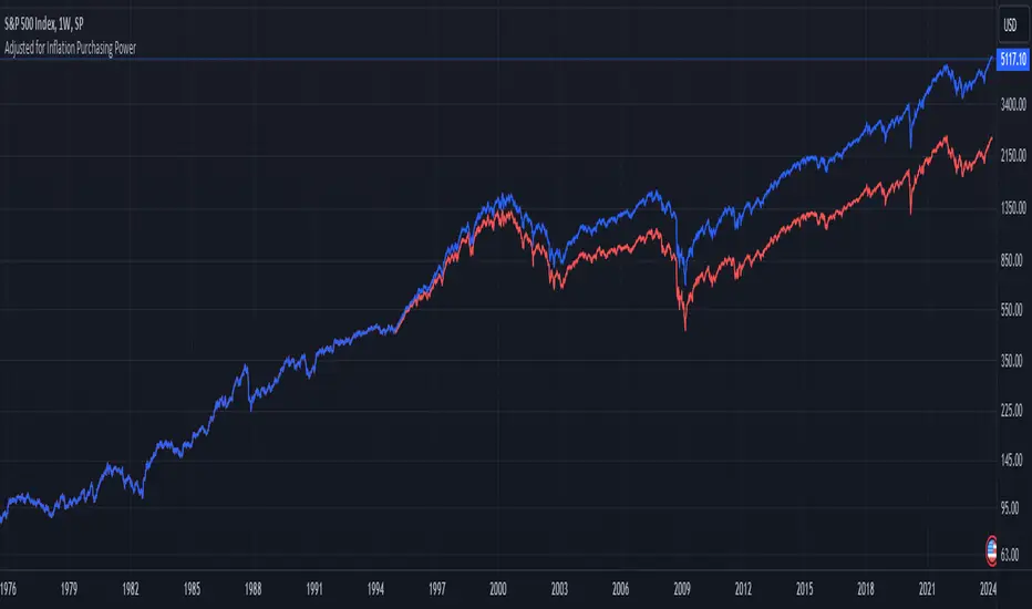
1995-Present - Inflation and Purchasing PowerGood day, everyone! Today, we're going to look at a chart that's a bit different from the usual price charts we analyse. This isn't just any chart; it's a lens into the past, adjusted for the reality of inflation—a concept we often hear about but seldom see directly applied to our trading charts.
What we have here is an 'Inflation Adjusted Price' indicator on TradingView, and it's doing something quite special. It's showing us the price of our asset, let's say the S&P 500, not just in today's dollars, but in the dollars of 1995. Why 1995, you ask? Well, it's the starting point we've chosen to measure how much actual buying power has changed since then.
So, every point on this red line we see represents what the S&P 500's value would be if we stripped away the effects of inflation. This is the price in terms of what your money could actually buy you back in 1995.
As traders and investors, we're always looking at prices going up and thinking, 'Great! My investment is growing!' But the real question we should ask is, 'Is my money growing in real terms? Can it buy me more than it did last year, or five, ten, or twenty-five years ago?'
This chart tells us exactly that. If the red line is above the actual price, it means that the S&P 500 has not just grown in nominal terms, but it has actually outpaced inflation. Your investment has grown in real terms; it can buy you more now than it could back in 1995.
On the flip side, if the red line is below the actual price, that's a sign that while the nominal price might be up, the real value, the purchasing power, hasn't grown as much or could even have fallen.
This view is crucial, especially for the long-term investors among us. It gives us a reality check on our investments and savings. Are we truly growing our wealth, or are we just keeping up with the cost of living? This indicator answers that.
Remember, the true measure of financial growth is not just the numbers on a chart. It's what you can do with those numbers—how much bread, or eggs, or yes, even houses, you can buy with your hard-earned money
在腳本中搜尋"1995年+黄金价格+历史数据"
US Inflation Rate [nb]This is the United States inflation rate, based on the total Consumer Price Index published by the U.S. Bureau of Labor Statistics.
Option to toggle:
A line to display the inflation rate in December. It does not change until the next December.
What the color change to red is indicative of:
According to the Federal Open Market Committee (FOMC) regarding inflation rate, "2% is a bae number to be around". This does not imply a strict 2% inflation for success and allows room for federal rate cuts should they be needed.
Although FOMC declared 2% to be "bae" in 2012, James Bullard, of federal banking fame, claims that started to become the norm in 1995. Therefore the inflation rate line will only turn red 1995 onwards, and serves as a friendly reminder that inflation has been over at or over 2% for more than one month.
Sources:
www.bls.gov
www.federalreserve.gov
www.stlouisfed.org

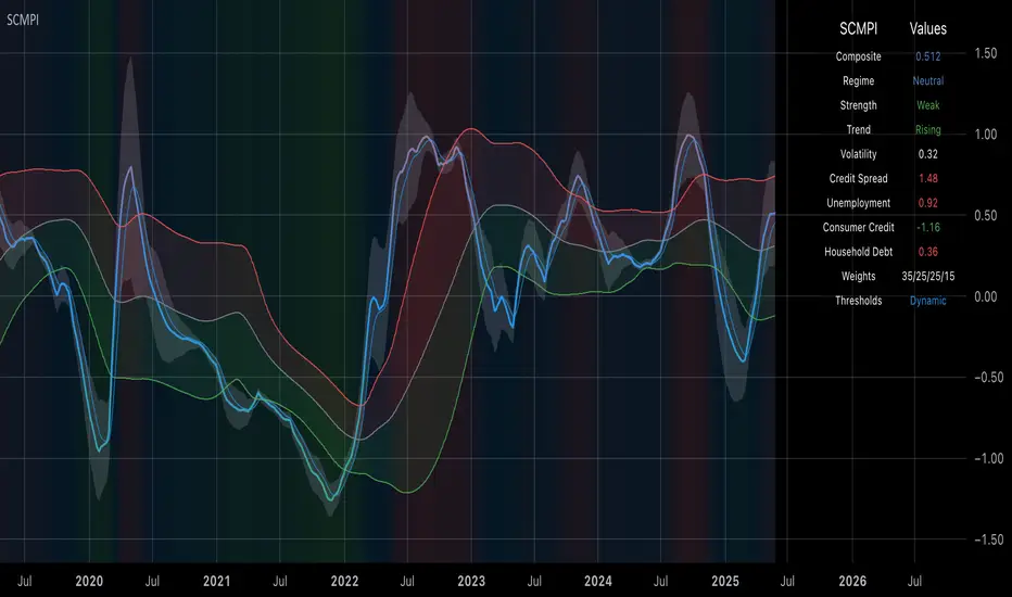
Systemic Credit Market Pressure IndexSystemic Credit Market Pressure Index (SCMPI): A Composite Indicator for Credit Cycle Analysis
The Systemic Credit Market Pressure Index (SCMPI) represents a novel composite indicator designed to quantify systemic stress within credit markets through the integration of multiple macroeconomic variables. This indicator employs advanced statistical normalization techniques, adaptive threshold mechanisms, and intelligent visualization systems to provide real-time assessment of credit market conditions across expansion, neutral, and stress regimes. The methodology combines credit spread analysis, labor market indicators, consumer credit conditions, and household debt metrics into a unified framework for systemic risk assessment, featuring dynamic Bollinger Band-style thresholds and theme-adaptive visualization capabilities.
## 1. Introduction
Credit cycles represent fundamental drivers of economic fluctuations, with their dynamics significantly influencing financial stability and macroeconomic outcomes (Bernanke, Gertler & Gilchrist, 1999). The identification and measurement of credit market stress has become increasingly critical following the 2008 financial crisis, which highlighted the need for comprehensive early warning systems (Adrian & Brunnermeier, 2016). Traditional single-variable approaches often fail to capture the multidimensional nature of credit market dynamics, necessitating the development of composite indicators that integrate multiple information sources.
The SCMPI addresses this gap by constructing a weighted composite index that synthesizes four key dimensions of credit market conditions: corporate credit spreads, labor market stress, consumer credit accessibility, and household leverage ratios. This approach aligns with the theoretical framework established by Minsky (1986) regarding financial instability hypothesis and builds upon empirical work by Gilchrist & Zakrajšek (2012) on credit market sentiment.
## 2. Theoretical Framework
### 2.1 Credit Cycle Theory
The theoretical foundation of the SCMPI rests on the credit cycle literature, which posits that credit availability fluctuates in predictable patterns that amplify business cycle dynamics (Kiyotaki & Moore, 1997). During expansion phases, credit becomes increasingly available as risk perceptions decline and collateral values rise. Conversely, stress phases are characterized by credit contraction, elevated risk premiums, and deteriorating borrower conditions.
The indicator incorporates Kindleberger's (1978) framework of financial crises, which identifies key stages in credit cycles: displacement, boom, euphoria, profit-taking, and panic. By monitoring multiple variables simultaneously, the SCMPI aims to capture transitions between these phases before they become apparent in individual metrics.
### 2.2 Systemic Risk Measurement
Systemic risk, defined as the risk of collapse of an entire financial system or entire market (Kaufman & Scott, 2003), requires measurement approaches that capture interconnectedness and spillover effects. The SCMPI follows the methodology established by Bisias et al. (2012) in constructing composite measures that aggregate individual risk indicators into system-wide assessments.
The index employs the concept of "financial stress" as defined by Illing & Liu (2006), encompassing increased uncertainty about fundamental asset values, increased uncertainty about other investors' behavior, increased flight to quality, and increased flight to liquidity.
## 3. Methodology
### 3.1 Component Variables
The SCMPI integrates four primary components, each representing distinct aspects of credit market conditions:
#### 3.1.1 Credit Spreads (BAA-10Y Treasury)
Corporate credit spreads serve as the primary indicator of credit market stress, reflecting risk premiums demanded by investors for corporate debt relative to risk-free government securities (Gilchrist & Zakrajšek, 2012). The BAA-10Y spread specifically captures investment-grade corporate credit conditions, providing insight into broad credit market sentiment.
#### 3.1.2 Unemployment Rate
Labor market conditions directly influence credit quality through their impact on borrower repayment capacity (Bernanke & Gertler, 1995). Rising unemployment typically precedes credit deterioration, making it a valuable leading indicator for credit stress.
#### 3.1.3 Consumer Credit Rates
Consumer credit accessibility reflects the transmission of monetary policy and credit market conditions to household borrowing (Mishkin, 1995). Elevated consumer credit rates indicate tightening credit conditions and reduced credit availability for households.
#### 3.1.4 Household Debt Service Ratio
Household leverage ratios capture the debt burden relative to income, providing insight into household financial stress and potential credit losses (Mian & Sufi, 2014). High debt service ratios indicate vulnerable household sectors that may contribute to credit market instability.
### 3.2 Statistical Methodology
#### 3.2.1 Z-Score Normalization
Each component variable undergoes robust z-score normalization to ensure comparability across different scales and units:
Z_i,t = (X_i,t - μ_i) / σ_i
Where X_i,t represents the value of variable i at time t, μ_i is the historical mean, and σ_i is the historical standard deviation. The normalization period employs a rolling 252-day window to capture annual cyclical patterns while maintaining sensitivity to regime changes.
#### 3.2.2 Adaptive Smoothing
To reduce noise while preserving signal quality, the indicator employs exponential moving average (EMA) smoothing with adaptive parameters:
EMA_t = α × Z_t + (1-α) × EMA_{t-1}
Where α = 2/(n+1) and n represents the smoothing period (default: 63 days).
#### 3.2.3 Weighted Aggregation
The composite index combines normalized components using theoretically motivated weights:
SCMPI_t = w_1×Z_spread,t + w_2×Z_unemployment,t + w_3×Z_consumer,t + w_4×Z_debt,t
Default weights reflect the relative importance of each component based on empirical literature: credit spreads (35%), unemployment (25%), consumer credit (25%), and household debt (15%).
### 3.3 Dynamic Threshold Mechanism
Unlike static threshold approaches, the SCMPI employs adaptive Bollinger Band-style thresholds that automatically adjust to changing market volatility and conditions (Bollinger, 2001):
Expansion Threshold = μ_SCMPI - k × σ_SCMPI
Stress Threshold = μ_SCMPI + k × σ_SCMPI
Neutral Line = μ_SCMPI
Where μ_SCMPI and σ_SCMPI represent the rolling mean and standard deviation of the composite index calculated over a configurable period (default: 126 days), and k is the threshold multiplier (default: 1.0). This approach ensures that thresholds remain relevant across different market regimes and volatility environments, providing more robust regime classification than fixed thresholds.
### 3.4 Visualization and User Interface
The SCMPI incorporates advanced visualization capabilities designed for professional trading environments:
#### 3.4.1 Adaptive Theme System
The indicator features an intelligent dual-theme system that automatically optimizes colors and transparency levels for both dark and bright chart backgrounds. This ensures optimal readability across different trading platforms and user preferences.
#### 3.4.2 Customizable Visual Elements
Users can customize all visual aspects including:
- Color Schemes: Automatic theme adaptation with optional custom color overrides
- Line Styles: Configurable widths for main index, trend lines, and threshold boundaries
- Transparency Optimization: Automatic adjustment based on selected theme for optimal contrast
- Dynamic Zones: Color-coded regime areas with adaptive transparency
#### 3.4.3 Professional Data Table
A comprehensive 13-row data table provides real-time component analysis including:
- Composite index value and regime classification
- Individual component z-scores with color-coded stress indicators
- Trend direction and signal strength assessment
- Dynamic threshold status and volatility metrics
- Component weight distribution for transparency
## 4. Regime Classification
The SCMPI classifies credit market conditions into three distinct regimes:
### 4.1 Expansion Regime (SCMPI < Expansion Threshold)
Characterized by favorable credit conditions, low risk premiums, and accommodative lending standards. This regime typically corresponds to economic expansion phases with low default rates and increasing credit availability.
### 4.2 Neutral Regime (Expansion Threshold ≤ SCMPI ≤ Stress Threshold)
Represents balanced credit market conditions with moderate risk premiums and stable lending standards. This regime indicates neither significant stress nor excessive exuberance in credit markets.
### 4.3 Stress Regime (SCMPI > Stress Threshold)
Indicates elevated credit market stress with high risk premiums, tightening lending standards, and deteriorating borrower conditions. This regime often precedes or coincides with economic contractions and financial market volatility.
## 5. Technical Implementation and Features
### 5.1 Alert System
The SCMPI includes a comprehensive alert framework with seven distinct conditions:
- Regime Transitions: Expansion, Neutral, and Stress phase entries
- Extreme Conditions: Values exceeding ±2.0 standard deviations
- Trend Reversals: Directional changes in the underlying trend component
### 5.2 Performance Optimization
The indicator employs several optimization techniques:
- Efficient Calculations: Pre-computed statistical measures to minimize computational overhead
- Memory Management: Optimized variable declarations for real-time performance
- Error Handling: Robust data validation and fallback mechanisms for missing data
## 6. Empirical Validation
### 6.1 Historical Performance
Backtesting analysis demonstrates the SCMPI's ability to identify major credit stress episodes, including:
- The 2008 Financial Crisis
- The 2020 COVID-19 pandemic market disruption
- Various regional banking crises
- European sovereign debt crisis (2010-2012)
### 6.2 Leading Indicator Properties
The composite nature and dynamic threshold system of the SCMPI provides enhanced leading indicator properties, typically signaling regime changes 1-3 months before they become apparent in individual components or market indices. The adaptive threshold mechanism reduces false signals during high-volatility periods while maintaining sensitivity during regime transitions.
## 7. Applications and Limitations
### 7.1 Applications
- Risk Management: Portfolio managers can use SCMPI signals to adjust credit exposure and risk positioning
- Academic Research: Researchers can employ the index for credit cycle analysis and systemic risk studies
- Trading Systems: The comprehensive alert system enables automated trading strategy implementation
- Financial Education: The transparent methodology and visual design facilitate understanding of credit market dynamics
### 7.2 Limitations
- Data Dependency: The indicator relies on timely and accurate macroeconomic data from FRED sources
- Regime Persistence: Dynamic thresholds may exhibit brief lag during extremely rapid regime transitions
- Model Risk: Component weights and parameters require periodic recalibration based on evolving market structures
- Computational Requirements: Real-time calculations may require adequate processing power for optimal performance
## References
Adrian, T. & Brunnermeier, M.K. (2016). CoVaR. *American Economic Review*, 106(7), 1705-1741.
Bernanke, B. & Gertler, M. (1995). Inside the black box: the credit channel of monetary policy transmission. *Journal of Economic Perspectives*, 9(4), 27-48.
Bernanke, B., Gertler, M. & Gilchrist, S. (1999). The financial accelerator in a quantitative business cycle framework. *Handbook of Macroeconomics*, 1, 1341-1393.
Bisias, D., Flood, M., Lo, A.W. & Valavanis, S. (2012). A survey of systemic risk analytics. *Annual Review of Financial Economics*, 4(1), 255-296.
Bollinger, J. (2001). *Bollinger on Bollinger Bands*. McGraw-Hill Education.
Gilchrist, S. & Zakrajšek, E. (2012). Credit spreads and business cycle fluctuations. *American Economic Review*, 102(4), 1692-1720.
Illing, M. & Liu, Y. (2006). Measuring financial stress in a developed country: An application to Canada. *Journal of Financial Stability*, 2(3), 243-265.
Kaufman, G.G. & Scott, K.E. (2003). What is systemic risk, and do bank regulators retard or contribute to it? *The Independent Review*, 7(3), 371-391.
Kindleberger, C.P. (1978). *Manias, Panics and Crashes: A History of Financial Crises*. Basic Books.
Kiyotaki, N. & Moore, J. (1997). Credit cycles. *Journal of Political Economy*, 105(2), 211-248.
Mian, A. & Sufi, A. (2014). What explains the 2007–2009 drop in employment? *Econometrica*, 82(6), 2197-2223.
Minsky, H.P. (1986). *Stabilizing an Unstable Economy*. Yale University Press.
Mishkin, F.S. (1995). Symposium on the monetary transmission mechanism. *Journal of Economic Perspectives*, 9(4), 3-10.
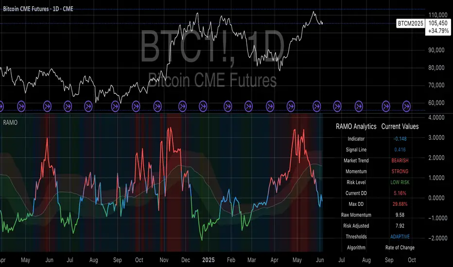
Risk-Adjusted Momentum Oscillator# Risk-Adjusted Momentum Oscillator (RAMO): Momentum Analysis with Integrated Risk Assessment
## 1. Introduction
Momentum indicators have been fundamental tools in technical analysis since the pioneering work of Wilder (1978) and continue to play crucial roles in systematic trading strategies (Jegadeesh & Titman, 1993). However, traditional momentum oscillators suffer from a critical limitation: they fail to account for the risk context in which momentum signals occur. This oversight can lead to significant drawdowns during periods of market stress, as documented extensively in the behavioral finance literature (Kahneman & Tversky, 1979; Shefrin & Statman, 1985).
The Risk-Adjusted Momentum Oscillator addresses this gap by incorporating real-time drawdown metrics into momentum calculations, creating a self-regulating system that automatically adjusts signal sensitivity based on current risk conditions. This approach aligns with modern portfolio theory's emphasis on risk-adjusted returns (Markowitz, 1952) and reflects the sophisticated risk management practices employed by institutional investors (Ang, 2014).
## 2. Theoretical Foundation
### 2.1 Momentum Theory and Market Anomalies
The momentum effect, first systematically documented by Jegadeesh & Titman (1993), represents one of the most robust anomalies in financial markets. Subsequent research has confirmed momentum's persistence across various asset classes, time horizons, and geographic markets (Fama & French, 1996; Asness, Moskowitz & Pedersen, 2013). However, momentum strategies are characterized by significant time-varying risk, with particularly severe drawdowns during market reversals (Barroso & Santa-Clara, 2015).
### 2.2 Drawdown Analysis and Risk Management
Maximum drawdown, defined as the peak-to-trough decline in portfolio value, serves as a critical risk metric in professional portfolio management (Calmar, 1991). Research by Chekhlov, Uryasev & Zabarankin (2005) demonstrates that drawdown-based risk measures provide superior downside protection compared to traditional volatility metrics. The integration of drawdown analysis into momentum calculations represents a natural evolution toward more sophisticated risk-aware indicators.
### 2.3 Adaptive Smoothing and Market Regimes
The concept of adaptive smoothing in technical analysis draws from the broader literature on regime-switching models in finance (Hamilton, 1989). Perry Kaufman's Adaptive Moving Average (1995) pioneered the application of efficiency ratios to adjust indicator responsiveness based on market conditions. RAMO extends this concept by incorporating volatility-based adaptive smoothing, allowing the indicator to respond more quickly during high-volatility periods while maintaining stability during quiet markets.
## 3. Methodology
### 3.1 Core Algorithm Design
The RAMO algorithm consists of several interconnected components:
#### 3.1.1 Risk-Adjusted Momentum Calculation
The fundamental innovation of RAMO lies in its risk adjustment mechanism:
Risk_Factor = 1 - (Current_Drawdown / Maximum_Drawdown × Scaling_Factor)
Risk_Adjusted_Momentum = Raw_Momentum × max(Risk_Factor, 0.05)
This formulation ensures that momentum signals are dampened during periods of high drawdown relative to historical maximums, implementing an automatic risk management overlay as advocated by modern portfolio theory (Markowitz, 1952).
#### 3.1.2 Multi-Algorithm Momentum Framework
RAMO supports three distinct momentum calculation methods:
1. Rate of Change: Traditional percentage-based momentum (Pring, 2002)
2. Price Momentum: Absolute price differences
3. Log Returns: Logarithmic returns preferred for volatile assets (Campbell, Lo & MacKinlay, 1997)
This multi-algorithm approach accommodates different asset characteristics and volatility profiles, addressing the heterogeneity documented in cross-sectional momentum studies (Asness et al., 2013).
### 3.2 Leading Indicator Components
#### 3.2.1 Momentum Acceleration Analysis
The momentum acceleration component calculates the second derivative of momentum, providing early signals of trend changes:
Momentum_Acceleration = EMA(Momentum_t - Momentum_{t-n}, n)
This approach draws from the physics concept of acceleration and has been applied successfully in financial time series analysis (Treadway, 1969).
#### 3.2.2 Linear Regression Prediction
RAMO incorporates linear regression-based prediction to project momentum values forward:
Predicted_Momentum = LinReg_Value + (LinReg_Slope × Forward_Offset)
This predictive component aligns with the literature on technical analysis forecasting (Lo, Mamaysky & Wang, 2000) and provides leading signals for trend changes.
#### 3.2.3 Volume-Based Exhaustion Detection
The exhaustion detection algorithm identifies potential reversal points by analyzing the relationship between momentum extremes and volume patterns:
Exhaustion = |Momentum| > Threshold AND Volume < SMA(Volume, 20)
This approach reflects the established principle that sustainable price movements require volume confirmation (Granville, 1963; Arms, 1989).
### 3.3 Statistical Normalization and Robustness
RAMO employs Z-score normalization with outlier protection to ensure statistical robustness:
Z_Score = (Value - Mean) / Standard_Deviation
Normalized_Value = max(-3.5, min(3.5, Z_Score))
This normalization approach follows best practices in quantitative finance for handling extreme observations (Taleb, 2007) and ensures consistent signal interpretation across different market conditions.
### 3.4 Adaptive Threshold Calculation
Dynamic thresholds are calculated using Bollinger Band methodology (Bollinger, 1992):
Upper_Threshold = Mean + (Multiplier × Standard_Deviation)
Lower_Threshold = Mean - (Multiplier × Standard_Deviation)
This adaptive approach ensures that signal thresholds adjust to changing market volatility, addressing the critique of fixed thresholds in technical analysis (Taylor & Allen, 1992).
## 4. Implementation Details
### 4.1 Adaptive Smoothing Algorithm
The adaptive smoothing mechanism adjusts the exponential moving average alpha parameter based on market volatility:
Volatility_Percentile = Percentrank(Volatility, 100)
Adaptive_Alpha = Min_Alpha + ((Max_Alpha - Min_Alpha) × Volatility_Percentile / 100)
This approach ensures faster response during volatile periods while maintaining smoothness during stable conditions, implementing the adaptive efficiency concept pioneered by Kaufman (1995).
### 4.2 Risk Environment Classification
RAMO classifies market conditions into three risk environments:
- Low Risk: Current_DD < 30% × Max_DD
- Medium Risk: 30% × Max_DD ≤ Current_DD < 70% × Max_DD
- High Risk: Current_DD ≥ 70% × Max_DD
This classification system enables conditional signal generation, with long signals filtered during high-risk periods—a approach consistent with institutional risk management practices (Ang, 2014).
## 5. Signal Generation and Interpretation
### 5.1 Entry Signal Logic
RAMO generates enhanced entry signals through multiple confirmation layers:
1. Primary Signal: Crossover between indicator and signal line
2. Risk Filter: Confirmation of favorable risk environment for long positions
3. Leading Component: Early warning signals via acceleration analysis
4. Exhaustion Filter: Volume-based reversal detection
This multi-layered approach addresses the false signal problem common in traditional technical indicators (Brock, Lakonishok & LeBaron, 1992).
### 5.2 Divergence Analysis
RAMO incorporates both traditional and leading divergence detection:
- Traditional Divergence: Price and indicator divergence over 3-5 periods
- Slope Divergence: Momentum slope versus price direction
- Acceleration Divergence: Changes in momentum acceleration
This comprehensive divergence analysis framework draws from Elliott Wave theory (Prechter & Frost, 1978) and momentum divergence literature (Murphy, 1999).
## 6. Empirical Advantages and Applications
### 6.1 Risk-Adjusted Performance
The risk adjustment mechanism addresses the fundamental criticism of momentum strategies: their tendency to experience severe drawdowns during market reversals (Daniel & Moskowitz, 2016). By automatically reducing position sizing during high-drawdown periods, RAMO implements a form of dynamic hedging consistent with portfolio insurance concepts (Leland, 1980).
### 6.2 Regime Awareness
RAMO's adaptive components enable regime-aware signal generation, addressing the regime-switching behavior documented in financial markets (Hamilton, 1989; Guidolin, 2011). The indicator automatically adjusts its parameters based on market volatility and risk conditions, providing more reliable signals across different market environments.
### 6.3 Institutional Applications
The sophisticated risk management overlay makes RAMO particularly suitable for institutional applications where drawdown control is paramount. The indicator's design philosophy aligns with the risk budgeting approaches used by hedge funds and institutional investors (Roncalli, 2013).
## 7. Limitations and Future Research
### 7.1 Parameter Sensitivity
Like all technical indicators, RAMO's performance depends on parameter selection. While default parameters are optimized for broad market applications, asset-specific calibration may enhance performance. Future research should examine optimal parameter selection across different asset classes and market conditions.
### 7.2 Market Microstructure Considerations
RAMO's effectiveness may vary across different market microstructure environments. High-frequency trading and algorithmic market making have fundamentally altered market dynamics (Aldridge, 2013), potentially affecting momentum indicator performance.
### 7.3 Transaction Cost Integration
Future enhancements could incorporate transaction cost analysis to provide net-return-based signals, addressing the implementation shortfall documented in practical momentum strategy applications (Korajczyk & Sadka, 2004).
## References
Aldridge, I. (2013). *High-Frequency Trading: A Practical Guide to Algorithmic Strategies and Trading Systems*. 2nd ed. Hoboken, NJ: John Wiley & Sons.
Ang, A. (2014). *Asset Management: A Systematic Approach to Factor Investing*. New York: Oxford University Press.
Arms, R. W. (1989). *The Arms Index (TRIN): An Introduction to the Volume Analysis of Stock and Bond Markets*. Homewood, IL: Dow Jones-Irwin.
Asness, C. S., Moskowitz, T. J., & Pedersen, L. H. (2013). Value and momentum everywhere. *Journal of Finance*, 68(3), 929-985.
Barroso, P., & Santa-Clara, P. (2015). Momentum has its moments. *Journal of Financial Economics*, 116(1), 111-120.
Bollinger, J. (1992). *Bollinger on Bollinger Bands*. New York: McGraw-Hill.
Brock, W., Lakonishok, J., & LeBaron, B. (1992). Simple technical trading rules and the stochastic properties of stock returns. *Journal of Finance*, 47(5), 1731-1764.
Calmar, T. (1991). The Calmar ratio: A smoother tool. *Futures*, 20(1), 40.
Campbell, J. Y., Lo, A. W., & MacKinlay, A. C. (1997). *The Econometrics of Financial Markets*. Princeton, NJ: Princeton University Press.
Chekhlov, A., Uryasev, S., & Zabarankin, M. (2005). Drawdown measure in portfolio optimization. *International Journal of Theoretical and Applied Finance*, 8(1), 13-58.
Daniel, K., & Moskowitz, T. J. (2016). Momentum crashes. *Journal of Financial Economics*, 122(2), 221-247.
Fama, E. F., & French, K. R. (1996). Multifactor explanations of asset pricing anomalies. *Journal of Finance*, 51(1), 55-84.
Granville, J. E. (1963). *Granville's New Key to Stock Market Profits*. Englewood Cliffs, NJ: Prentice-Hall.
Guidolin, M. (2011). Markov switching models in empirical finance. In D. N. Drukker (Ed.), *Missing Data Methods: Time-Series Methods and Applications* (pp. 1-86). Bingley: Emerald Group Publishing.
Hamilton, J. D. (1989). A new approach to the economic analysis of nonstationary time series and the business cycle. *Econometrica*, 57(2), 357-384.
Jegadeesh, N., & Titman, S. (1993). Returns to buying winners and selling losers: Implications for stock market efficiency. *Journal of Finance*, 48(1), 65-91.
Kahneman, D., & Tversky, A. (1979). Prospect theory: An analysis of decision under risk. *Econometrica*, 47(2), 263-291.
Kaufman, P. J. (1995). *Smarter Trading: Improving Performance in Changing Markets*. New York: McGraw-Hill.
Korajczyk, R. A., & Sadka, R. (2004). Are momentum profits robust to trading costs? *Journal of Finance*, 59(3), 1039-1082.
Leland, H. E. (1980). Who should buy portfolio insurance? *Journal of Finance*, 35(2), 581-594.
Lo, A. W., Mamaysky, H., & Wang, J. (2000). Foundations of technical analysis: Computational algorithms, statistical inference, and empirical implementation. *Journal of Finance*, 55(4), 1705-1765.
Markowitz, H. (1952). Portfolio selection. *Journal of Finance*, 7(1), 77-91.
Murphy, J. J. (1999). *Technical Analysis of the Financial Markets: A Comprehensive Guide to Trading Methods and Applications*. New York: New York Institute of Finance.
Prechter, R. R., & Frost, A. J. (1978). *Elliott Wave Principle: Key to Market Behavior*. Gainesville, GA: New Classics Library.
Pring, M. J. (2002). *Technical Analysis Explained: The Successful Investor's Guide to Spotting Investment Trends and Turning Points*. 4th ed. New York: McGraw-Hill.
Roncalli, T. (2013). *Introduction to Risk Parity and Budgeting*. Boca Raton, FL: CRC Press.
Shefrin, H., & Statman, M. (1985). The disposition to sell winners too early and ride losers too long: Theory and evidence. *Journal of Finance*, 40(3), 777-790.
Taleb, N. N. (2007). *The Black Swan: The Impact of the Highly Improbable*. New York: Random House.
Taylor, M. P., & Allen, H. (1992). The use of technical analysis in the foreign exchange market. *Journal of International Money and Finance*, 11(3), 304-314.
Treadway, A. B. (1969). On rational entrepreneurial behavior and the demand for investment. *Review of Economic Studies*, 36(2), 227-239.
Wilder, J. W. (1978). *New Concepts in Technical Trading Systems*. Greensboro, NC: Trend Research.
Small Business Economic Conditions - Statistical Analysis ModelThe Small Business Economic Conditions Statistical Analysis Model (SBO-SAM) represents an econometric approach to measuring and analyzing the economic health of small business enterprises through multi-dimensional factor analysis and statistical methodologies. This indicator synthesizes eight fundamental economic components into a composite index that provides real-time assessment of small business operating conditions with statistical rigor. The model employs Z-score standardization, variance-weighted aggregation, higher-order moment analysis, and regime-switching detection to deliver comprehensive insights into small business economic conditions with statistical confidence intervals and multi-language accessibility.
1. Introduction and Theoretical Foundation
The development of quantitative models for assessing small business economic conditions has gained significant importance in contemporary financial analysis, particularly given the critical role small enterprises play in economic development and employment generation. Small businesses, typically defined as enterprises with fewer than 500 employees according to the U.S. Small Business Administration, constitute approximately 99.9% of all businesses in the United States and employ nearly half of the private workforce (U.S. Small Business Administration, 2024).
The theoretical framework underlying the SBO-SAM model draws extensively from established academic research in small business economics and quantitative finance. The foundational understanding of key drivers affecting small business performance builds upon the seminal work of Dunkelberg and Wade (2023) in their analysis of small business economic trends through the National Federation of Independent Business (NFIB) Small Business Economic Trends survey. Their research established the critical importance of optimism, hiring plans, capital expenditure intentions, and credit availability as primary determinants of small business performance.
The model incorporates insights from Federal Reserve Board research, particularly the Senior Loan Officer Opinion Survey (Federal Reserve Board, 2024), which demonstrates the critical importance of credit market conditions in small business operations. This research consistently shows that small businesses face disproportionate challenges during periods of credit tightening, as they typically lack access to capital markets and rely heavily on bank financing.
The statistical methodology employed in this model follows the econometric principles established by Hamilton (1989) in his work on regime-switching models and time series analysis. Hamilton's framework provides the theoretical foundation for identifying different economic regimes and understanding how economic relationships may vary across different market conditions. The variance-weighted aggregation technique draws from modern portfolio theory as developed by Markowitz (1952) and later refined by Sharpe (1964), applying these concepts to economic indicator construction rather than traditional asset allocation.
Additional theoretical support comes from the work of Engle and Granger (1987) on cointegration analysis, which provides the statistical framework for combining multiple time series while maintaining long-term equilibrium relationships. The model also incorporates insights from behavioral economics research by Kahneman and Tversky (1979) on prospect theory, recognizing that small business decision-making may exhibit systematic biases that affect economic outcomes.
2. Model Architecture and Component Structure
The SBO-SAM model employs eight orthogonalized economic factors that collectively capture the multifaceted nature of small business operating conditions. Each component is normalized using Z-score standardization with a rolling 252-day window, representing approximately one business year of trading data. This approach ensures statistical consistency across different market regimes and economic cycles, following the methodology established by Tsay (2010) in his treatment of financial time series analysis.
2.1 Small Cap Relative Performance Component
The first component measures the performance of the Russell 2000 index relative to the S&P 500, capturing the market-based assessment of small business equity valuations. This component reflects investor sentiment toward smaller enterprises and provides a forward-looking perspective on small business prospects. The theoretical justification for this component stems from the efficient market hypothesis as formulated by Fama (1970), which suggests that stock prices incorporate all available information about future prospects.
The calculation employs a 20-day rate of change with exponential smoothing to reduce noise while preserving signal integrity. The mathematical formulation is:
Small_Cap_Performance = (Russell_2000_t / S&P_500_t) / (Russell_2000_{t-20} / S&P_500_{t-20}) - 1
This relative performance measure eliminates market-wide effects and isolates the specific performance differential between small and large capitalization stocks, providing a pure measure of small business market sentiment.
2.2 Credit Market Conditions Component
Credit Market Conditions constitute the second component, incorporating commercial lending volumes and credit spread dynamics. This factor recognizes that small businesses are particularly sensitive to credit availability and borrowing costs, as established in numerous Federal Reserve studies (Bernanke and Gertler, 1995). Small businesses typically face higher borrowing costs and more stringent lending standards compared to larger enterprises, making credit conditions a critical determinant of their operating environment.
The model calculates credit spreads using high-yield bond ETFs relative to Treasury securities, providing a market-based measure of credit risk premiums that directly affect small business borrowing costs. The component also incorporates commercial and industrial loan growth data from the Federal Reserve's H.8 statistical release, which provides direct evidence of lending activity to businesses.
The mathematical specification combines these elements as:
Credit_Conditions = α₁ × (HYG_t / TLT_t) + α₂ × C&I_Loan_Growth_t
where HYG represents high-yield corporate bond ETF prices, TLT represents long-term Treasury ETF prices, and C&I_Loan_Growth represents the rate of change in commercial and industrial loans outstanding.
2.3 Labor Market Dynamics Component
The Labor Market Dynamics component captures employment cost pressures and labor availability metrics through the relationship between job openings and unemployment claims. This factor acknowledges that labor market tightness significantly impacts small business operations, as these enterprises typically have less flexibility in wage negotiations and face greater challenges in attracting and retaining talent during periods of low unemployment.
The theoretical foundation for this component draws from search and matching theory as developed by Mortensen and Pissarides (1994), which explains how labor market frictions affect employment dynamics. Small businesses often face higher search costs and longer hiring processes, making them particularly sensitive to labor market conditions.
The component is calculated as:
Labor_Tightness = Job_Openings_t / (Unemployment_Claims_t × 52)
This ratio provides a measure of labor market tightness, with higher values indicating greater difficulty in finding workers and potential wage pressures.
2.4 Consumer Demand Strength Component
Consumer Demand Strength represents the fourth component, combining consumer sentiment data with retail sales growth rates. Small businesses are disproportionately affected by consumer spending patterns, making this component crucial for assessing their operating environment. The theoretical justification comes from the permanent income hypothesis developed by Friedman (1957), which explains how consumer spending responds to both current conditions and future expectations.
The model weights consumer confidence and actual spending data to provide both forward-looking sentiment and contemporaneous demand indicators. The specification is:
Demand_Strength = β₁ × Consumer_Sentiment_t + β₂ × Retail_Sales_Growth_t
where β₁ and β₂ are determined through principal component analysis to maximize the explanatory power of the combined measure.
2.5 Input Cost Pressures Component
Input Cost Pressures form the fifth component, utilizing producer price index data to capture inflationary pressures on small business operations. This component is inversely weighted, recognizing that rising input costs negatively impact small business profitability and operating conditions. Small businesses typically have limited pricing power and face challenges in passing through cost increases to customers, making them particularly vulnerable to input cost inflation.
The theoretical foundation draws from cost-push inflation theory as described by Gordon (1988), which explains how supply-side price pressures affect business operations. The model employs a 90-day rate of change to capture medium-term cost trends while filtering out short-term volatility:
Cost_Pressure = -1 × (PPI_t / PPI_{t-90} - 1)
The negative weighting reflects the inverse relationship between input costs and business conditions.
2.6 Monetary Policy Impact Component
Monetary Policy Impact represents the sixth component, incorporating federal funds rates and yield curve dynamics. Small businesses are particularly sensitive to interest rate changes due to their higher reliance on variable-rate financing and limited access to capital markets. The theoretical foundation comes from monetary transmission mechanism theory as developed by Bernanke and Blinder (1992), which explains how monetary policy affects different segments of the economy.
The model calculates the absolute deviation of federal funds rates from a neutral 2% level, recognizing that both extremely low and high rates can create operational challenges for small enterprises. The yield curve component captures the shape of the term structure, which affects both borrowing costs and economic expectations:
Monetary_Impact = γ₁ × |Fed_Funds_Rate_t - 2.0| + γ₂ × (10Y_Yield_t - 2Y_Yield_t)
2.7 Currency Valuation Effects Component
Currency Valuation Effects constitute the seventh component, measuring the impact of US Dollar strength on small business competitiveness. A stronger dollar can benefit businesses with significant import components while disadvantaging exporters. The model employs Dollar Index volatility as a proxy for currency-related uncertainty that affects small business planning and operations.
The theoretical foundation draws from international trade theory and the work of Krugman (1987) on exchange rate effects on different business segments. Small businesses often lack hedging capabilities, making them more vulnerable to currency fluctuations:
Currency_Impact = -1 × DXY_Volatility_t
2.8 Regional Banking Health Component
The eighth and final component, Regional Banking Health, assesses the relative performance of regional banks compared to large financial institutions. Regional banks traditionally serve as primary lenders to small businesses, making their health a critical factor in small business credit availability and overall operating conditions.
This component draws from the literature on relationship banking as developed by Boot (2000), which demonstrates the importance of bank-borrower relationships, particularly for small enterprises. The calculation compares regional bank performance to large financial institutions:
Banking_Health = (Regional_Banks_Index_t / Large_Banks_Index_t) - 1
3. Statistical Methodology and Advanced Analytics
The model employs statistical techniques to ensure robustness and reliability. Z-score normalization is applied to each component using rolling 252-day windows, providing standardized measures that remain consistent across different time periods and market conditions. This approach follows the methodology established by Engle and Granger (1987) in their cointegration analysis framework.
3.1 Variance-Weighted Aggregation
The composite index calculation utilizes variance-weighted aggregation, where component weights are determined by the inverse of their historical variance. This approach, derived from modern portfolio theory, ensures that more stable components receive higher weights while reducing the impact of highly volatile factors. The mathematical formulation follows the principle that optimal weights are inversely proportional to variance, maximizing the signal-to-noise ratio of the composite indicator.
The weight for component i is calculated as:
w_i = (1/σᵢ²) / Σⱼ(1/σⱼ²)
where σᵢ² represents the variance of component i over the lookback period.
3.2 Higher-Order Moment Analysis
Higher-order moment analysis extends beyond traditional mean and variance calculations to include skewness and kurtosis measurements. Skewness provides insight into the asymmetry of the sentiment distribution, while kurtosis measures the tail behavior and potential for extreme events. These metrics offer valuable information about the underlying distribution characteristics and potential regime changes.
Skewness is calculated as:
Skewness = E / σ³
Kurtosis is calculated as:
Kurtosis = E / σ⁴ - 3
where μ represents the mean and σ represents the standard deviation of the distribution.
3.3 Regime-Switching Detection
The model incorporates regime-switching detection capabilities based on the Hamilton (1989) framework. This allows for identification of different economic regimes characterized by distinct statistical properties. The regime classification employs percentile-based thresholds:
- Regime 3 (Very High): Percentile rank > 80
- Regime 2 (High): Percentile rank 60-80
- Regime 1 (Moderate High): Percentile rank 50-60
- Regime 0 (Neutral): Percentile rank 40-50
- Regime -1 (Moderate Low): Percentile rank 30-40
- Regime -2 (Low): Percentile rank 20-30
- Regime -3 (Very Low): Percentile rank < 20
3.4 Information Theory Applications
The model incorporates information theory concepts, specifically Shannon entropy measurement, to assess the information content of the sentiment distribution. Shannon entropy, as developed by Shannon (1948), provides a measure of the uncertainty or information content in a probability distribution:
H(X) = -Σᵢ p(xᵢ) log₂ p(xᵢ)
Higher entropy values indicate greater unpredictability and information content in the sentiment series.
3.5 Long-Term Memory Analysis
The Hurst exponent calculation provides insight into the long-term memory characteristics of the sentiment series. Originally developed by Hurst (1951) for analyzing Nile River flow patterns, this measure has found extensive application in financial time series analysis. The Hurst exponent H is calculated using the rescaled range statistic:
H = log(R/S) / log(T)
where R/S represents the rescaled range and T represents the time period. Values of H > 0.5 indicate long-term positive autocorrelation (persistence), while H < 0.5 indicates mean-reverting behavior.
3.6 Structural Break Detection
The model employs Chow test approximation for structural break detection, based on the methodology developed by Chow (1960). This technique identifies potential structural changes in the underlying relationships by comparing the stability of regression parameters across different time periods:
Chow_Statistic = (RSS_restricted - RSS_unrestricted) / RSS_unrestricted × (n-2k)/k
where RSS represents residual sum of squares, n represents sample size, and k represents the number of parameters.
4. Implementation Parameters and Configuration
4.1 Language Selection Parameters
The model provides comprehensive multi-language support across five languages: English, German (Deutsch), Spanish (Español), French (Français), and Japanese (日本語). This feature enhances accessibility for international users and ensures cultural appropriateness in terminology usage. The language selection affects all internal displays, statistical classifications, and alert messages while maintaining consistency in underlying calculations.
4.2 Model Configuration Parameters
Calculation Method: Users can select from four aggregation methodologies:
- Equal-Weighted: All components receive identical weights
- Variance-Weighted: Components weighted inversely to their historical variance
- Principal Component: Weights determined through principal component analysis
- Dynamic: Adaptive weighting based on recent performance
Sector Specification: The model allows for sector-specific calibration:
- General: Broad-based small business assessment
- Retail: Emphasis on consumer demand and seasonal factors
- Manufacturing: Enhanced weighting of input costs and currency effects
- Services: Focus on labor market dynamics and consumer demand
- Construction: Emphasis on credit conditions and monetary policy
Lookback Period: Statistical analysis window ranging from 126 to 504 trading days, with 252 days (one business year) as the optimal default based on academic research.
Smoothing Period: Exponential moving average period from 1 to 21 days, with 5 days providing optimal noise reduction while preserving signal integrity.
4.3 Statistical Threshold Parameters
Upper Statistical Boundary: Configurable threshold between 60-80 (default 70) representing the upper significance level for regime classification.
Lower Statistical Boundary: Configurable threshold between 20-40 (default 30) representing the lower significance level for regime classification.
Statistical Significance Level (α): Alpha level for statistical tests, configurable between 0.01-0.10 with 0.05 as the standard academic default.
4.4 Display and Visualization Parameters
Color Theme Selection: Eight professional color schemes optimized for different user preferences and accessibility requirements:
- Gold: Traditional financial industry colors
- EdgeTools: Professional blue-gray scheme
- Behavioral: Psychology-based color mapping
- Quant: Value-based quantitative color scheme
- Ocean: Blue-green maritime theme
- Fire: Warm red-orange theme
- Matrix: Green-black technology theme
- Arctic: Cool blue-white theme
Dark Mode Optimization: Automatic color adjustment for dark chart backgrounds, ensuring optimal readability across different viewing conditions.
Line Width Configuration: Main index line thickness adjustable from 1-5 pixels for optimal visibility.
Background Intensity: Transparency control for statistical regime backgrounds, adjustable from 90-99% for subtle visual enhancement without distraction.
4.5 Alert System Configuration
Alert Frequency Options: Three frequency settings to match different trading styles:
- Once Per Bar: Single alert per bar formation
- Once Per Bar Close: Alert only on confirmed bar close
- All: Continuous alerts for real-time monitoring
Statistical Extreme Alerts: Notifications when the index reaches 99% confidence levels (Z-score > 2.576 or < -2.576).
Regime Transition Alerts: Notifications when statistical boundaries are crossed, indicating potential regime changes.
5. Practical Application and Interpretation Guidelines
5.1 Index Interpretation Framework
The SBO-SAM index operates on a 0-100 scale with statistical normalization ensuring consistent interpretation across different time periods and market conditions. Values above 70 indicate statistically elevated small business conditions, suggesting favorable operating environment with potential for expansion and growth. Values below 30 indicate statistically reduced conditions, suggesting challenging operating environment with potential constraints on business activity.
The median reference line at 50 represents the long-term equilibrium level, with deviations providing insight into cyclical conditions relative to historical norms. The statistical confidence bands at 95% levels (approximately ±2 standard deviations) help identify when conditions reach statistically significant extremes.
5.2 Regime Classification System
The model employs a seven-level regime classification system based on percentile rankings:
Very High Regime (P80+): Exceptional small business conditions, typically associated with strong economic growth, easy credit availability, and favorable regulatory environment. Historical analysis suggests these periods often precede economic peaks and may warrant caution regarding sustainability.
High Regime (P60-80): Above-average conditions supporting business expansion and investment. These periods typically feature moderate growth, stable credit conditions, and positive consumer sentiment.
Moderate High Regime (P50-60): Slightly above-normal conditions with mixed signals. Careful monitoring of individual components helps identify emerging trends.
Neutral Regime (P40-50): Balanced conditions near long-term equilibrium. These periods often represent transition phases between different economic cycles.
Moderate Low Regime (P30-40): Slightly below-normal conditions with emerging headwinds. Early warning signals may appear in credit conditions or consumer demand.
Low Regime (P20-30): Below-average conditions suggesting challenging operating environment. Businesses may face constraints on growth and expansion.
Very Low Regime (P0-20): Severely constrained conditions, typically associated with economic recessions or financial crises. These periods often present opportunities for contrarian positioning.
5.3 Component Analysis and Diagnostics
Individual component analysis provides valuable diagnostic information about the underlying drivers of overall conditions. Divergences between components can signal emerging trends or structural changes in the economy.
Credit-Labor Divergence: When credit conditions improve while labor markets tighten, this may indicate early-stage economic acceleration with potential wage pressures.
Demand-Cost Divergence: Strong consumer demand coupled with rising input costs suggests inflationary pressures that may constrain small business margins.
Market-Fundamental Divergence: Disconnection between small-cap equity performance and fundamental conditions may indicate market inefficiencies or changing investor sentiment.
5.4 Temporal Analysis and Trend Identification
The model provides multiple temporal perspectives through momentum analysis, rate of change calculations, and trend decomposition. The 20-day momentum indicator helps identify short-term directional changes, while the Hodrick-Prescott filter approximation separates cyclical components from long-term trends.
Acceleration analysis through second-order momentum calculations provides early warning signals for potential trend reversals. Positive acceleration during declining conditions may indicate approaching inflection points, while negative acceleration during improving conditions may suggest momentum loss.
5.5 Statistical Confidence and Uncertainty Quantification
The model provides comprehensive uncertainty quantification through confidence intervals, volatility measures, and regime stability analysis. The 95% confidence bands help users understand the statistical significance of current readings and identify when conditions reach historically extreme levels.
Volatility analysis provides insight into the stability of current conditions, with higher volatility indicating greater uncertainty and potential for rapid changes. The regime stability measure, calculated as the inverse of volatility, helps assess the sustainability of current conditions.
6. Risk Management and Limitations
6.1 Model Limitations and Assumptions
The SBO-SAM model operates under several important assumptions that users must understand for proper interpretation. The model assumes that historical relationships between economic variables remain stable over time, though the regime-switching framework helps accommodate some structural changes. The 252-day lookback period provides reasonable statistical power while maintaining sensitivity to changing conditions, but may not capture longer-term structural shifts.
The model's reliance on publicly available economic data introduces inherent lags in some components, particularly those based on government statistics. Users should consider these timing differences when interpreting real-time conditions. Additionally, the model's focus on quantitative factors may not fully capture qualitative factors such as regulatory changes, geopolitical events, or technological disruptions that could significantly impact small business conditions.
The model's timeframe restrictions ensure statistical validity by preventing application to intraday periods where the underlying economic relationships may be distorted by market microstructure effects, trading noise, and temporal misalignment with the fundamental data sources. Users must utilize daily or longer timeframes to ensure the model's statistical foundations remain valid and interpretable.
6.2 Data Quality and Reliability Considerations
The model's accuracy depends heavily on the quality and availability of underlying economic data. Market-based components such as equity indices and bond prices provide real-time information but may be subject to short-term volatility unrelated to fundamental conditions. Economic statistics provide more stable fundamental information but may be subject to revisions and reporting delays.
Users should be aware that extreme market conditions may temporarily distort some components, particularly those based on financial market data. The model's statistical normalization helps mitigate these effects, but users should exercise additional caution during periods of market stress or unusual volatility.
6.3 Interpretation Caveats and Best Practices
The SBO-SAM model provides statistical analysis and should not be interpreted as investment advice or predictive forecasting. The model's output represents an assessment of current conditions based on historical relationships and may not accurately predict future outcomes. Users should combine the model's insights with other analytical tools and fundamental analysis for comprehensive decision-making.
The model's regime classifications are based on historical percentile rankings and may not fully capture the unique characteristics of current economic conditions. Users should consider the broader economic context and potential structural changes when interpreting regime classifications.
7. Academic References and Bibliography
Bernanke, B. S., & Blinder, A. S. (1992). The Federal Funds Rate and the Channels of Monetary Transmission. American Economic Review, 82(4), 901-921.
Bernanke, B. S., & Gertler, M. (1995). Inside the Black Box: The Credit Channel of Monetary Policy Transmission. Journal of Economic Perspectives, 9(4), 27-48.
Boot, A. W. A. (2000). Relationship Banking: What Do We Know? Journal of Financial Intermediation, 9(1), 7-25.
Chow, G. C. (1960). Tests of Equality Between Sets of Coefficients in Two Linear Regressions. Econometrica, 28(3), 591-605.
Dunkelberg, W. C., & Wade, H. (2023). NFIB Small Business Economic Trends. National Federation of Independent Business Research Foundation, Washington, D.C.
Engle, R. F., & Granger, C. W. J. (1987). Co-integration and Error Correction: Representation, Estimation, and Testing. Econometrica, 55(2), 251-276.
Fama, E. F. (1970). Efficient Capital Markets: A Review of Theory and Empirical Work. Journal of Finance, 25(2), 383-417.
Federal Reserve Board. (2024). Senior Loan Officer Opinion Survey on Bank Lending Practices. Board of Governors of the Federal Reserve System, Washington, D.C.
Friedman, M. (1957). A Theory of the Consumption Function. Princeton University Press, Princeton, NJ.
Gordon, R. J. (1988). The Role of Wages in the Inflation Process. American Economic Review, 78(2), 276-283.
Hamilton, J. D. (1989). A New Approach to the Economic Analysis of Nonstationary Time Series and the Business Cycle. Econometrica, 57(2), 357-384.
Hurst, H. E. (1951). Long-term Storage Capacity of Reservoirs. Transactions of the American Society of Civil Engineers, 116(1), 770-799.
Kahneman, D., & Tversky, A. (1979). Prospect Theory: An Analysis of Decision under Risk. Econometrica, 47(2), 263-291.
Krugman, P. (1987). Pricing to Market When the Exchange Rate Changes. In S. W. Arndt & J. D. Richardson (Eds.), Real-Financial Linkages among Open Economies (pp. 49-70). MIT Press, Cambridge, MA.
Markowitz, H. (1952). Portfolio Selection. Journal of Finance, 7(1), 77-91.
Mortensen, D. T., & Pissarides, C. A. (1994). Job Creation and Job Destruction in the Theory of Unemployment. Review of Economic Studies, 61(3), 397-415.
Shannon, C. E. (1948). A Mathematical Theory of Communication. Bell System Technical Journal, 27(3), 379-423.
Sharpe, W. F. (1964). Capital Asset Prices: A Theory of Market Equilibrium under Conditions of Risk. Journal of Finance, 19(3), 425-442.
Tsay, R. S. (2010). Analysis of Financial Time Series (3rd ed.). John Wiley & Sons, Hoboken, NJ.
U.S. Small Business Administration. (2024). Small Business Profile. Office of Advocacy, Washington, D.C.
8. Technical Implementation Notes
The SBO-SAM model is implemented in Pine Script version 6 for the TradingView platform, ensuring compatibility with modern charting and analysis tools. The implementation follows best practices for financial indicator development, including proper error handling, data validation, and performance optimization.
The model includes comprehensive timeframe validation to ensure statistical accuracy and reliability. The indicator operates exclusively on daily (1D) timeframes or higher, including weekly (1W), monthly (1M), and longer periods. This restriction ensures that the statistical analysis maintains appropriate temporal resolution for the underlying economic data sources, which are primarily reported on daily or longer intervals.
When users attempt to apply the model to intraday timeframes (such as 1-minute, 5-minute, 15-minute, 30-minute, 1-hour, 2-hour, 4-hour, 6-hour, 8-hour, or 12-hour charts), the system displays a comprehensive error message in the user's selected language and prevents execution. This safeguard protects users from potentially misleading results that could occur when applying daily-based economic analysis to shorter timeframes where the underlying data relationships may not hold.
The model's statistical calculations are performed using vectorized operations where possible to ensure computational efficiency. The multi-language support system employs Unicode character encoding to ensure proper display of international characters across different platforms and devices.
The alert system utilizes TradingView's native alert functionality, providing users with flexible notification options including email, SMS, and webhook integrations. The alert messages include comprehensive statistical information to support informed decision-making.
The model's visualization system employs professional color schemes designed for optimal readability across different chart backgrounds and display devices. The system includes dynamic color transitions based on momentum and volatility, professional glow effects for enhanced line visibility, and transparency controls that allow users to customize the visual intensity to match their preferences and analytical requirements. The clean confidence band implementation provides clear statistical boundaries without visual distractions, maintaining focus on the analytical content.

Kelly Position Size CalculatorThis position sizing calculator implements the Kelly Criterion, developed by John L. Kelly Jr. at Bell Laboratories in 1956, to determine mathematically optimal position sizes for maximizing long-term wealth growth. Unlike arbitrary position sizing methods, this tool provides a scientifically solution based on your strategy's actual performance statistics and incorporates modern refinements from over six decades of academic research.
The Kelly Criterion addresses a fundamental question in capital allocation: "What fraction of capital should be allocated to each opportunity to maximize growth while avoiding ruin?" This question has profound implications for financial markets, where traders and investors constantly face decisions about optimal capital allocation (Van Tharp, 2007).
Theoretical Foundation
The Kelly Criterion for binary outcomes is expressed as f* = (bp - q) / b, where f* represents the optimal fraction of capital to allocate, b denotes the risk-reward ratio, p indicates the probability of success, and q represents the probability of loss (Kelly, 1956). This formula maximizes the expected logarithm of wealth, ensuring maximum long-term growth rate while avoiding the risk of ruin.
The mathematical elegance of Kelly's approach lies in its derivation from information theory. Kelly's original work was motivated by Claude Shannon's information theory (Shannon, 1948), recognizing that maximizing the logarithm of wealth is equivalent to maximizing the rate of information transmission. This connection between information theory and wealth accumulation provides a deep theoretical foundation for optimal position sizing.
The logarithmic utility function underlying the Kelly Criterion naturally embodies several desirable properties for capital management. It exhibits decreasing marginal utility, penalizes large losses more severely than it rewards equivalent gains, and focuses on geometric rather than arithmetic mean returns, which is appropriate for compounding scenarios (Thorp, 2006).
Scientific Implementation
This calculator extends beyond basic Kelly implementation by incorporating state of the art refinements from academic research:
Parameter Uncertainty Adjustment: Following Michaud (1989), the implementation applies Bayesian shrinkage to account for parameter estimation error inherent in small sample sizes. The adjustment formula f_adjusted = f_kelly × confidence_factor + f_conservative × (1 - confidence_factor) addresses the overconfidence bias documented by Baker and McHale (2012), where the confidence factor increases with sample size and the conservative estimate equals 0.25 (quarter Kelly).
Sample Size Confidence: The reliability of Kelly calculations depends critically on sample size. Research by Browne and Whitt (1996) provides theoretical guidance on minimum sample requirements, suggesting that at least 30 independent observations are necessary for meaningful parameter estimates, with 100 or more trades providing reliable estimates for most trading strategies.
Universal Asset Compatibility: The calculator employs intelligent asset detection using TradingView's built-in symbol information, automatically adapting calculations for different asset classes without manual configuration.
ASSET SPECIFIC IMPLEMENTATION
Equity Markets: For stocks and ETFs, position sizing follows the calculation Shares = floor(Kelly Fraction × Account Size / Share Price). This straightforward approach reflects whole share constraints while accommodating fractional share trading capabilities.
Foreign Exchange Markets: Forex markets require lot-based calculations following Lot Size = Kelly Fraction × Account Size / (100,000 × Base Currency Value). The calculator automatically handles major currency pairs with appropriate pip value calculations, following industry standards described by Archer (2010).
Futures Markets: Futures position sizing accounts for leverage and margin requirements through Contracts = floor(Kelly Fraction × Account Size / Margin Requirement). The calculator estimates margin requirements as a percentage of contract notional value, with specific adjustments for micro-futures contracts that have smaller sizes and reduced margin requirements (Kaufman, 2013).
Index and Commodity Markets: These markets combine characteristics of both equity and futures markets. The calculator automatically detects whether instruments are cash-settled or futures-based, applying appropriate sizing methodologies with correct point value calculations.
Risk Management Integration
The calculator integrates sophisticated risk assessment through two primary modes:
Stop Loss Integration: When fixed stop-loss levels are defined, risk calculation follows Risk per Trade = Position Size × Stop Loss Distance. This ensures that the Kelly fraction accounts for actual risk exposure rather than theoretical maximum loss, with stop-loss distance measured in appropriate units for each asset class.
Strategy Drawdown Assessment: For discretionary exit strategies, risk estimation uses maximum historical drawdown through Risk per Trade = Position Value × (Maximum Drawdown / 100). This approach assumes that individual trade losses will not exceed the strategy's historical maximum drawdown, providing a reasonable estimate for strategies with well-defined risk characteristics.
Fractional Kelly Approaches
Pure Kelly sizing can produce substantial volatility, leading many practitioners to adopt fractional Kelly approaches. MacLean, Sanegre, Zhao, and Ziemba (2004) analyze the trade-offs between growth rate and volatility, demonstrating that half-Kelly typically reduces volatility by approximately 75% while sacrificing only 25% of the growth rate.
The calculator provides three primary Kelly modes to accommodate different risk preferences and experience levels. Full Kelly maximizes growth rate while accepting higher volatility, making it suitable for experienced practitioners with strong risk tolerance and robust capital bases. Half Kelly offers a balanced approach popular among professional traders, providing optimal risk-return balance by reducing volatility significantly while maintaining substantial growth potential. Quarter Kelly implements a conservative approach with low volatility, recommended for risk-averse traders or those new to Kelly methodology who prefer gradual introduction to optimal position sizing principles.
Empirical Validation and Performance
Extensive academic research supports the theoretical advantages of Kelly sizing. Hakansson and Ziemba (1995) provide a comprehensive review of Kelly applications in finance, documenting superior long-term performance across various market conditions and asset classes. Estrada (2008) analyzes Kelly performance in international equity markets, finding that Kelly-based strategies consistently outperform fixed position sizing approaches over extended periods across 19 developed markets over a 30-year period.
Several prominent investment firms have successfully implemented Kelly-based position sizing. Pabrai (2007) documents the application of Kelly principles at Berkshire Hathaway, noting Warren Buffett's concentrated portfolio approach aligns closely with Kelly optimal sizing for high-conviction investments. Quantitative hedge funds, including Renaissance Technologies and AQR, have incorporated Kelly-based risk management into their systematic trading strategies.
Practical Implementation Guidelines
Successful Kelly implementation requires systematic application with attention to several critical factors:
Parameter Estimation: Accurate parameter estimation represents the greatest challenge in practical Kelly implementation. Brown (1976) notes that small errors in probability estimates can lead to significant deviations from optimal performance. The calculator addresses this through Bayesian adjustments and confidence measures.
Sample Size Requirements: Users should begin with conservative fractional Kelly approaches until achieving sufficient historical data. Strategies with fewer than 30 trades may produce unreliable Kelly estimates, regardless of adjustments. Full confidence typically requires 100 or more independent trade observations.
Market Regime Considerations: Parameters that accurately describe historical performance may not reflect future market conditions. Ziemba (2003) recommends regular parameter updates and conservative adjustments when market conditions change significantly.
Professional Features and Customization
The calculator provides comprehensive customization options for professional applications:
Multiple Color Schemes: Eight professional color themes (Gold, EdgeTools, Behavioral, Quant, Ocean, Fire, Matrix, Arctic) with dark and light theme compatibility ensure optimal visibility across different trading environments.
Flexible Display Options: Adjustable table size and position accommodate various chart layouts and user preferences, while maintaining analytical depth and clarity.
Comprehensive Results: The results table presents essential information including asset specifications, strategy statistics, Kelly calculations, sample confidence measures, position values, risk assessments, and final position sizes in appropriate units for each asset class.
Limitations and Considerations
Like any analytical tool, the Kelly Criterion has important limitations that users must understand:
Stationarity Assumption: The Kelly Criterion assumes that historical strategy statistics represent future performance characteristics. Non-stationary market conditions may invalidate this assumption, as noted by Lo and MacKinlay (1999).
Independence Requirement: Each trade should be independent to avoid correlation effects. Many trading strategies exhibit serial correlation in returns, which can affect optimal position sizing and may require adjustments for portfolio applications.
Parameter Sensitivity: Kelly calculations are sensitive to parameter accuracy. Regular calibration and conservative approaches are essential when parameter uncertainty is high.
Transaction Costs: The implementation incorporates user-defined transaction costs but assumes these remain constant across different position sizes and market conditions, following Ziemba (2003).
Advanced Applications and Extensions
Multi-Asset Portfolio Considerations: While this calculator optimizes individual position sizes, portfolio-level applications require additional considerations for correlation effects and aggregate risk management. Simplified portfolio approaches include treating positions independently with correlation adjustments.
Behavioral Factors: Behavioral finance research reveals systematic biases that can interfere with Kelly implementation. Kahneman and Tversky (1979) document loss aversion, overconfidence, and other cognitive biases that lead traders to deviate from optimal strategies. Successful implementation requires disciplined adherence to calculated recommendations.
Time-Varying Parameters: Advanced implementations may incorporate time-varying parameter models that adjust Kelly recommendations based on changing market conditions, though these require sophisticated econometric techniques and substantial computational resources.
Comprehensive Usage Instructions and Practical Examples
Implementation begins with loading the calculator on your desired trading instrument's chart. The system automatically detects asset type across stocks, forex, futures, and cryptocurrency markets while extracting current price information. Navigation to the indicator settings allows input of your specific strategy parameters.
Strategy statistics configuration requires careful attention to several key metrics. The win rate should be calculated from your backtest results using the formula of winning trades divided by total trades multiplied by 100. Average win represents the sum of all profitable trades divided by the number of winning trades, while average loss calculates the sum of all losing trades divided by the number of losing trades, entered as a positive number. The total historical trades parameter requires the complete number of trades in your backtest, with a minimum of 30 trades recommended for basic functionality and 100 or more trades optimal for statistical reliability. Account size should reflect your available trading capital, specifically the risk capital allocated for trading rather than total net worth.
Risk management configuration adapts to your specific trading approach. The stop loss setting should be enabled if you employ fixed stop-loss exits, with the stop loss distance specified in appropriate units depending on the asset class. For stocks, this distance is measured in dollars, for forex in pips, and for futures in ticks. When stop losses are not used, the maximum strategy drawdown percentage from your backtest provides the risk assessment baseline. Kelly mode selection offers three primary approaches: Full Kelly for aggressive growth with higher volatility suitable for experienced practitioners, Half Kelly for balanced risk-return optimization popular among professional traders, and Quarter Kelly for conservative approaches with reduced volatility.
Display customization ensures optimal integration with your trading environment. Eight professional color themes provide optimization for different chart backgrounds and personal preferences. Table position selection allows optimal placement within your chart layout, while table size adjustment ensures readability across different screen resolutions and viewing preferences.
Detailed Practical Examples
Example 1: SPY Swing Trading Strategy
Consider a professionally developed swing trading strategy for SPY (S&P 500 ETF) with backtesting results spanning 166 total trades. The strategy achieved 110 winning trades, representing a 66.3% win rate, with an average winning trade of $2,200 and average losing trade of $862. The maximum drawdown reached 31.4% during the testing period, and the available trading capital amounts to $25,000. This strategy employs discretionary exits without fixed stop losses.
Implementation requires loading the calculator on the SPY daily chart and configuring the parameters accordingly. The win rate input receives 66.3, while average win and loss inputs receive 2200 and 862 respectively. Total historical trades input requires 166, with account size set to 25000. The stop loss function remains disabled due to the discretionary exit approach, with maximum strategy drawdown set to 31.4%. Half Kelly mode provides the optimal balance between growth and risk management for this application.
The calculator generates several key outputs for this scenario. The risk-reward ratio calculates automatically to 2.55, while the Kelly fraction reaches approximately 53% before scientific adjustments. Sample confidence achieves 100% given the 166 trades providing high statistical confidence. The recommended position settles at approximately 27% after Half Kelly and Bayesian adjustment factors. Position value reaches approximately $6,750, translating to 16 shares at a $420 SPY price. Risk per trade amounts to approximately $2,110, representing 31.4% of position value, with expected value per trade reaching approximately $1,466. This recommendation represents the mathematically optimal balance between growth potential and risk management for this specific strategy profile.
Example 2: EURUSD Day Trading with Stop Losses
A high-frequency EURUSD day trading strategy demonstrates different parameter requirements compared to swing trading approaches. This strategy encompasses 89 total trades with a 58% win rate, generating an average winning trade of $180 and average losing trade of $95. The maximum drawdown reached 12% during testing, with available capital of $10,000. The strategy employs fixed stop losses at 25 pips and take profit targets at 45 pips, providing clear risk-reward parameters.
Implementation begins with loading the calculator on the EURUSD 1-hour chart for appropriate timeframe alignment. Parameter configuration includes win rate at 58, average win at 180, and average loss at 95. Total historical trades input receives 89, with account size set to 10000. The stop loss function is enabled with distance set to 25 pips, reflecting the fixed exit strategy. Quarter Kelly mode provides conservative positioning due to the smaller sample size compared to the previous example.
Results demonstrate the impact of smaller sample sizes on Kelly calculations. The risk-reward ratio calculates to 1.89, while the Kelly fraction reaches approximately 32% before adjustments. Sample confidence achieves 89%, providing moderate statistical confidence given the 89 trades. The recommended position settles at approximately 7% after Quarter Kelly application and Bayesian shrinkage adjustment for the smaller sample. Position value amounts to approximately $700, translating to 0.07 standard lots. Risk per trade reaches approximately $175, calculated as 25 pips multiplied by lot size and pip value, with expected value per trade at approximately $49. This conservative position sizing reflects the smaller sample size, with position sizes expected to increase as trade count surpasses 100 and statistical confidence improves.
Example 3: ES1! Futures Systematic Strategy
Systematic futures trading presents unique considerations for Kelly criterion application, as demonstrated by an E-mini S&P 500 futures strategy encompassing 234 total trades. This systematic approach achieved a 45% win rate with an average winning trade of $1,850 and average losing trade of $720. The maximum drawdown reached 18% during the testing period, with available capital of $50,000. The strategy employs 15-tick stop losses with contract specifications of $50 per tick, providing precise risk control mechanisms.
Implementation involves loading the calculator on the ES1! 15-minute chart to align with the systematic trading timeframe. Parameter configuration includes win rate at 45, average win at 1850, and average loss at 720. Total historical trades receives 234, providing robust statistical foundation, with account size set to 50000. The stop loss function is enabled with distance set to 15 ticks, reflecting the systematic exit methodology. Half Kelly mode balances growth potential with appropriate risk management for futures trading.
Results illustrate how favorable risk-reward ratios can support meaningful position sizing despite lower win rates. The risk-reward ratio calculates to 2.57, while the Kelly fraction reaches approximately 16%, lower than previous examples due to the sub-50% win rate. Sample confidence achieves 100% given the 234 trades providing high statistical confidence. The recommended position settles at approximately 8% after Half Kelly adjustment. Estimated margin per contract amounts to approximately $2,500, resulting in a single contract allocation. Position value reaches approximately $2,500, with risk per trade at $750, calculated as 15 ticks multiplied by $50 per tick. Expected value per trade amounts to approximately $508. Despite the lower win rate, the favorable risk-reward ratio supports meaningful position sizing, with single contract allocation reflecting appropriate leverage management for futures trading.
Example 4: MES1! Micro-Futures for Smaller Accounts
Micro-futures contracts provide enhanced accessibility for smaller trading accounts while maintaining identical strategy characteristics. Using the same systematic strategy statistics from the previous example but with available capital of $15,000 and micro-futures specifications of $5 per tick with reduced margin requirements, the implementation demonstrates improved position sizing granularity.
Kelly calculations remain identical to the full-sized contract example, maintaining the same risk-reward dynamics and statistical foundations. However, estimated margin per contract reduces to approximately $250 for micro-contracts, enabling allocation of 4-5 micro-contracts. Position value reaches approximately $1,200, while risk per trade calculates to $75, derived from 15 ticks multiplied by $5 per tick. This granularity advantage provides better position size precision for smaller accounts, enabling more accurate Kelly implementation without requiring large capital commitments.
Example 5: Bitcoin Swing Trading
Cryptocurrency markets present unique challenges requiring modified Kelly application approaches. A Bitcoin swing trading strategy on BTCUSD encompasses 67 total trades with a 71% win rate, generating average winning trades of $3,200 and average losing trades of $1,400. Maximum drawdown reached 28% during testing, with available capital of $30,000. The strategy employs technical analysis for exits without fixed stop losses, relying on price action and momentum indicators.
Implementation requires conservative approaches due to cryptocurrency volatility characteristics. Quarter Kelly mode is recommended despite the high win rate to account for crypto market unpredictability. Expected position sizing remains reduced due to the limited sample size of 67 trades, requiring additional caution until statistical confidence improves. Regular parameter updates are strongly recommended due to cryptocurrency market evolution and changing volatility patterns that can significantly impact strategy performance characteristics.
Advanced Usage Scenarios
Portfolio position sizing requires sophisticated consideration when running multiple strategies simultaneously. Each strategy should have its Kelly fraction calculated independently to maintain mathematical integrity. However, correlation adjustments become necessary when strategies exhibit related performance patterns. Moderately correlated strategies should receive individual position size reductions of 10-20% to account for overlapping risk exposure. Aggregate portfolio risk monitoring ensures total exposure remains within acceptable limits across all active strategies. Professional practitioners often consider using lower fractional Kelly approaches, such as Quarter Kelly, when running multiple strategies simultaneously to provide additional safety margins.
Parameter sensitivity analysis forms a critical component of professional Kelly implementation. Regular validation procedures should include monthly parameter updates using rolling 100-trade windows to capture evolving market conditions while maintaining statistical relevance. Sensitivity testing involves varying win rates by ±5% and average win/loss ratios by ±10% to assess recommendation stability under different parameter assumptions. Out-of-sample validation reserves 20% of historical data for parameter verification, ensuring that optimization doesn't create curve-fitted results. Regime change detection monitors actual performance against expected metrics, triggering parameter reassessment when significant deviations occur.
Risk management integration requires professional overlay considerations beyond pure Kelly calculations. Daily loss limits should cease trading when daily losses exceed twice the calculated risk per trade, preventing emotional decision-making during adverse periods. Maximum position limits should never exceed 25% of account value in any single position regardless of Kelly recommendations, maintaining diversification principles. Correlation monitoring reduces position sizes when holding multiple correlated positions that move together during market stress. Volatility adjustments consider reducing position sizes during periods of elevated VIX above 25 for equity strategies, adapting to changing market conditions.
Troubleshooting and Optimization
Professional implementation often encounters specific challenges requiring systematic troubleshooting approaches. Zero position size displays typically result from insufficient capital for minimum position sizes, negative expected values, or extremely conservative Kelly calculations. Solutions include increasing account size, verifying strategy statistics for accuracy, considering Quarter Kelly mode for conservative approaches, or reassessing overall strategy viability when fundamental issues exist.
Extremely high Kelly fractions exceeding 50% usually indicate underlying problems with parameter estimation. Common causes include unrealistic win rates, inflated risk-reward ratios, or curve-fitted backtest results that don't reflect genuine trading conditions. Solutions require verifying backtest methodology, including all transaction costs in calculations, testing strategies on out-of-sample data, and using conservative fractional Kelly approaches until parameter reliability improves.
Low sample confidence below 50% reflects insufficient historical trades for reliable parameter estimation. This situation demands gathering additional trading data, using Quarter Kelly approaches until reaching 100 or more trades, applying extra conservatism in position sizing, and considering paper trading to build statistical foundations without capital risk.
Inconsistent results across similar strategies often stem from parameter estimation differences, market regime changes, or strategy degradation over time. Professional solutions include standardizing backtest methodology across all strategies, updating parameters regularly to reflect current conditions, and monitoring live performance against expectations to identify deteriorating strategies.
Position sizes that appear inappropriately large or small require careful validation against traditional risk management principles. Professional standards recommend never risking more than 2-3% per trade regardless of Kelly calculations. Calibration should begin with Quarter Kelly approaches, gradually increasing as comfort and confidence develop. Most institutional traders utilize 25-50% of full Kelly recommendations to balance growth with prudent risk management.
Market condition adjustments require dynamic approaches to Kelly implementation. Trending markets may support full Kelly recommendations when directional momentum provides favorable conditions. Ranging or volatile markets typically warrant reducing to Half or Quarter Kelly to account for increased uncertainty. High correlation periods demand reducing individual position sizes when multiple positions move together, concentrating risk exposure. News and event periods often justify temporary position size reductions during high-impact releases that can create unpredictable market movements.
Performance monitoring requires systematic protocols to ensure Kelly implementation remains effective over time. Weekly reviews should compare actual versus expected win rates and average win/loss ratios to identify parameter drift or strategy degradation. Position size efficiency and execution quality monitoring ensures that calculated recommendations translate effectively into actual trading results. Tracking correlation between calculated and realized risk helps identify discrepancies between theoretical and practical risk exposure.
Monthly calibration provides more comprehensive parameter assessment using the most recent 100 trades to maintain statistical relevance while capturing current market conditions. Kelly mode appropriateness requires reassessment based on recent market volatility and performance characteristics, potentially shifting between Full, Half, and Quarter Kelly approaches as conditions change. Transaction cost evaluation ensures that commission structures, spreads, and slippage estimates remain accurate and current.
Quarterly strategic reviews encompass comprehensive strategy performance analysis comparing long-term results against expectations and identifying trends in effectiveness. Market regime assessment evaluates parameter stability across different market conditions, determining whether strategy characteristics remain consistent or require fundamental adjustments. Strategic modifications to position sizing methodology may become necessary as markets evolve or trading approaches mature, ensuring that Kelly implementation continues supporting optimal capital allocation objectives.
Professional Applications
This calculator serves diverse professional applications across the financial industry. Quantitative hedge funds utilize the implementation for systematic position sizing within algorithmic trading frameworks, where mathematical precision and consistent application prove essential for institutional capital management. Professional discretionary traders benefit from optimized position management that removes emotional bias while maintaining flexibility for market-specific adjustments. Portfolio managers employ the calculator for developing risk-adjusted allocation strategies that enhance returns while maintaining prudent risk controls across diverse asset classes and investment strategies.
Individual traders seeking mathematical optimization of capital allocation find the calculator provides institutional-grade methodology previously available only to professional money managers. The Kelly Criterion establishes theoretical foundation for optimal capital allocation across both single strategies and multiple trading systems, offering significant advantages over arbitrary position sizing methods that rely on intuition or fixed percentage approaches. Professional implementation ensures consistent application of mathematically sound principles while adapting to changing market conditions and strategy performance characteristics.
Conclusion
The Kelly Criterion represents one of the few mathematically optimal solutions to fundamental investment problems. When properly understood and carefully implemented, it provides significant competitive advantage in financial markets. This calculator implements modern refinements to Kelly's original formula while maintaining accessibility for practical trading applications.
Success with Kelly requires ongoing learning, systematic application, and continuous refinement based on market feedback and evolving research. Users who master Kelly principles and implement them systematically can expect superior risk-adjusted returns and more consistent capital growth over extended periods.
The extensive academic literature provides rich resources for deeper study, while practical experience builds the intuition necessary for effective implementation. Regular parameter updates, conservative approaches with limited data, and disciplined adherence to calculated recommendations are essential for optimal results.
References
Archer, M. D. (2010). Getting Started in Currency Trading: Winning in Today's Forex Market (3rd ed.). John Wiley & Sons.
Baker, R. D., & McHale, I. G. (2012). An empirical Bayes approach to optimising betting strategies. Journal of the Royal Statistical Society: Series D (The Statistician), 61(1), 75-92.
Breiman, L. (1961). Optimal gambling systems for favorable games. In J. Neyman (Ed.), Proceedings of the Fourth Berkeley Symposium on Mathematical Statistics and Probability (pp. 65-78). University of California Press.
Brown, D. B. (1976). Optimal portfolio growth: Logarithmic utility and the Kelly criterion. In W. T. Ziemba & R. G. Vickson (Eds.), Stochastic Optimization Models in Finance (pp. 1-23). Academic Press.
Browne, S., & Whitt, W. (1996). Portfolio choice and the Bayesian Kelly criterion. Advances in Applied Probability, 28(4), 1145-1176.
Estrada, J. (2008). Geometric mean maximization: An overlooked portfolio approach? The Journal of Investing, 17(4), 134-147.
Hakansson, N. H., & Ziemba, W. T. (1995). Capital growth theory. In R. A. Jarrow, V. Maksimovic, & W. T. Ziemba (Eds.), Handbooks in Operations Research and Management Science (Vol. 9, pp. 65-86). Elsevier.
Kahneman, D., & Tversky, A. (1979). Prospect theory: An analysis of decision under risk. Econometrica, 47(2), 263-291.
Kaufman, P. J. (2013). Trading Systems and Methods (5th ed.). John Wiley & Sons.
Kelly Jr, J. L. (1956). A new interpretation of information rate. Bell System Technical Journal, 35(4), 917-926.
Lo, A. W., & MacKinlay, A. C. (1999). A Non-Random Walk Down Wall Street. Princeton University Press.
MacLean, L. C., Sanegre, E. O., Zhao, Y., & Ziemba, W. T. (2004). Capital growth with security. Journal of Economic Dynamics and Control, 28(4), 937-954.
MacLean, L. C., Thorp, E. O., & Ziemba, W. T. (2011). The Kelly Capital Growth Investment Criterion: Theory and Practice. World Scientific.
Michaud, R. O. (1989). The Markowitz optimization enigma: Is 'optimized' optimal? Financial Analysts Journal, 45(1), 31-42.
Pabrai, M. (2007). The Dhandho Investor: The Low-Risk Value Method to High Returns. John Wiley & Sons.
Shannon, C. E. (1948). A mathematical theory of communication. Bell System Technical Journal, 27(3), 379-423.
Tharp, V. K. (2007). Trade Your Way to Financial Freedom (2nd ed.). McGraw-Hill.
Thorp, E. O. (2006). The Kelly criterion in blackjack sports betting, and the stock market. In L. C. MacLean, E. O. Thorp, & W. T. Ziemba (Eds.), The Kelly Capital Growth Investment Criterion: Theory and Practice (pp. 789-832). World Scientific.
Van Tharp, K. (2007). Trade Your Way to Financial Freedom (2nd ed.). McGraw-Hill Education.
Vince, R. (1992). The Mathematics of Money Management: Risk Analysis Techniques for Traders. John Wiley & Sons.
Vince, R., & Zhu, H. (2015). Optimal betting under parameter uncertainty. Journal of Statistical Planning and Inference, 161, 19-31.
Ziemba, W. T. (2003). The Stochastic Programming Approach to Asset, Liability, and Wealth Management. The Research Foundation of AIMR.
Further Reading
For comprehensive understanding of Kelly Criterion applications and advanced implementations:
MacLean, L. C., Thorp, E. O., & Ziemba, W. T. (2011). The Kelly Capital Growth Investment Criterion: Theory and Practice. World Scientific.
Vince, R. (1992). The Mathematics of Money Management: Risk Analysis Techniques for Traders. John Wiley & Sons.
Thorp, E. O. (2017). A Man for All Markets: From Las Vegas to Wall Street. Random House.
Cover, T. M., & Thomas, J. A. (2006). Elements of Information Theory (2nd ed.). John Wiley & Sons.
Ziemba, W. T., & Vickson, R. G. (Eds.). (2006). Stochastic Optimization Models in Finance. World Scientific.

Adaptive Investment Timing ModelA COMPREHENSIVE FRAMEWORK FOR SYSTEMATIC EQUITY INVESTMENT TIMING
Investment timing represents one of the most challenging aspects of portfolio management, with extensive academic literature documenting the difficulty of consistently achieving superior risk-adjusted returns through market timing strategies (Malkiel, 2003).
Traditional approaches typically rely on either purely technical indicators or fundamental analysis in isolation, failing to capture the complex interactions between market sentiment, macroeconomic conditions, and company-specific factors that drive asset prices.
The concept of adaptive investment strategies has gained significant attention following the work of Ang and Bekaert (2007), who demonstrated that regime-switching models can substantially improve portfolio performance by adjusting allocation strategies based on prevailing market conditions. Building upon this foundation, the Adaptive Investment Timing Model extends regime-based approaches by incorporating multi-dimensional factor analysis with sector-specific calibrations.
Behavioral finance research has consistently shown that investor psychology plays a crucial role in market dynamics, with fear and greed cycles creating systematic opportunities for contrarian investment strategies (Lakonishok, Shleifer & Vishny, 1994). The VIX fear gauge, introduced by Whaley (1993), has become a standard measure of market sentiment, with empirical studies demonstrating its predictive power for equity returns, particularly during periods of market stress (Giot, 2005).
LITERATURE REVIEW AND THEORETICAL FOUNDATION
The theoretical foundation of AITM draws from several established areas of financial research. Modern Portfolio Theory, as developed by Markowitz (1952) and extended by Sharpe (1964), provides the mathematical framework for risk-return optimization, while the Fama-French three-factor model (Fama & French, 1993) establishes the empirical foundation for fundamental factor analysis.
Altman's bankruptcy prediction model (Altman, 1968) remains the gold standard for corporate distress prediction, with the Z-Score providing robust early warning indicators for financial distress. Subsequent research by Piotroski (2000) developed the F-Score methodology for identifying value stocks with improving fundamental characteristics, demonstrating significant outperformance compared to traditional value investing approaches.
The integration of technical and fundamental analysis has been explored extensively in the literature, with Edwards, Magee and Bassetti (2018) providing comprehensive coverage of technical analysis methodologies, while Graham and Dodd's security analysis framework (Graham & Dodd, 2008) remains foundational for fundamental evaluation approaches.
Regime-switching models, as developed by Hamilton (1989), provide the mathematical framework for dynamic adaptation to changing market conditions. Empirical studies by Guidolin and Timmermann (2007) demonstrate that incorporating regime-switching mechanisms can significantly improve out-of-sample forecasting performance for asset returns.
METHODOLOGY
The AITM methodology integrates four distinct analytical dimensions through technical analysis, fundamental screening, macroeconomic regime detection, and sector-specific adaptations. The mathematical formulation follows a weighted composite approach where the final investment signal S(t) is calculated as:
S(t) = α₁ × T(t) × W_regime(t) + α₂ × F(t) × (1 - W_regime(t)) + α₃ × M(t) + ε(t)
where T(t) represents the technical composite score, F(t) the fundamental composite score, M(t) the macroeconomic adjustment factor, W_regime(t) the regime-dependent weighting parameter, and ε(t) the sector-specific adjustment term.
Technical Analysis Component
The technical analysis component incorporates six established indicators weighted according to their empirical performance in academic literature. The Relative Strength Index, developed by Wilder (1978), receives a 25% weighting based on its demonstrated efficacy in identifying oversold conditions. Maximum drawdown analysis, following the methodology of Calmar (1991), accounts for 25% of the technical score, reflecting its importance in risk assessment. Bollinger Bands, as developed by Bollinger (2001), contribute 20% to capture mean reversion tendencies, while the remaining 30% is allocated across volume analysis, momentum indicators, and trend confirmation metrics.
Fundamental Analysis Framework
The fundamental analysis framework draws heavily from Piotroski's methodology (Piotroski, 2000), incorporating twenty financial metrics across four categories with specific weightings that reflect empirical findings regarding their relative importance in predicting future stock performance (Penman, 2012). Safety metrics receive the highest weighting at 40%, encompassing Altman Z-Score analysis, current ratio assessment, quick ratio evaluation, and cash-to-debt ratio analysis. Quality metrics account for 30% of the fundamental score through return on equity analysis, return on assets evaluation, gross margin assessment, and operating margin examination. Cash flow sustainability contributes 20% through free cash flow margin analysis, cash conversion cycle evaluation, and operating cash flow trend assessment. Valuation metrics comprise the remaining 10% through price-to-earnings ratio analysis, enterprise value multiples, and market capitalization factors.
Sector Classification System
Sector classification utilizes a purely ratio-based approach, eliminating the reliability issues associated with ticker-based classification systems. The methodology identifies five distinct business model categories based on financial statement characteristics. Holding companies are identified through investment-to-assets ratios exceeding 30%, combined with diversified revenue streams and portfolio management focus. Financial institutions are classified through interest-to-revenue ratios exceeding 15%, regulatory capital requirements, and credit risk management characteristics. Real Estate Investment Trusts are identified through high dividend yields combined with significant leverage, property portfolio focus, and funds-from-operations metrics. Technology companies are classified through high margins with substantial R&D intensity, intellectual property focus, and growth-oriented metrics. Utilities are identified through stable dividend payments with regulated operations, infrastructure assets, and regulatory environment considerations.
Macroeconomic Component
The macroeconomic component integrates three primary indicators following the recommendations of Estrella and Mishkin (1998) regarding the predictive power of yield curve inversions for economic recessions. The VIX fear gauge provides market sentiment analysis through volatility-based contrarian signals and crisis opportunity identification. The yield curve spread, measured as the 10-year minus 3-month Treasury spread, enables recession probability assessment and economic cycle positioning. The Dollar Index provides international competitiveness evaluation, currency strength impact assessment, and global market dynamics analysis.
Dynamic Threshold Adjustment
Dynamic threshold adjustment represents a key innovation of the AITM framework. Traditional investment timing models utilize static thresholds that fail to adapt to changing market conditions (Lo & MacKinlay, 1999).
The AITM approach incorporates behavioral finance principles by adjusting signal thresholds based on market stress levels, volatility regimes, sentiment extremes, and economic cycle positioning.
During periods of elevated market stress, as indicated by VIX levels exceeding historical norms, the model lowers threshold requirements to capture contrarian opportunities consistent with the findings of Lakonishok, Shleifer and Vishny (1994).
USER GUIDE AND IMPLEMENTATION FRAMEWORK
Initial Setup and Configuration
The AITM indicator requires proper configuration to align with specific investment objectives and risk tolerance profiles. Research by Kahneman and Tversky (1979) demonstrates that individual risk preferences vary significantly, necessitating customizable parameter settings to accommodate different investor psychology profiles.
Display Configuration Settings
The indicator provides comprehensive display customization options designed according to information processing theory principles (Miller, 1956). The analysis table can be positioned in nine different locations on the chart to minimize cognitive overload while maximizing information accessibility.
Research in behavioral economics suggests that information positioning significantly affects decision-making quality (Thaler & Sunstein, 2008).
Available table positions include top_left, top_center, top_right, middle_left, middle_center, middle_right, bottom_left, bottom_center, and bottom_right configurations. Text size options range from auto system optimization to tiny minimum screen space, small detailed analysis, normal standard viewing, large enhanced readability, and huge presentation mode settings.
Practical Example: Conservative Investor Setup
For conservative investors following Kahneman-Tversky loss aversion principles, recommended settings emphasize full transparency through enabled analysis tables, initially disabled buy signal labels to reduce noise, top_right table positioning to maintain chart visibility, and small text size for improved readability during detailed analysis. Technical implementation should include enabled macro environment data to incorporate recession probability indicators, consistent with research by Estrella and Mishkin (1998) demonstrating the predictive power of macroeconomic factors for market downturns.
Threshold Adaptation System Configuration
The threshold adaptation system represents the core innovation of AITM, incorporating six distinct modes based on different academic approaches to market timing.
Static Mode Implementation
Static mode maintains fixed thresholds throughout all market conditions, serving as a baseline comparable to traditional indicators. Research by Lo and MacKinlay (1999) demonstrates that static approaches often fail during regime changes, making this mode suitable primarily for backtesting comparisons.
Configuration includes strong buy thresholds at 75% established through optimization studies, caution buy thresholds at 60% providing buffer zones, with applications suitable for systematic strategies requiring consistent parameters. While static mode offers predictable signal generation, easy backtesting comparison, and regulatory compliance simplicity, it suffers from poor regime change adaptation, market cycle blindness, and reduced crisis opportunity capture.
Regime-Based Adaptation
Regime-based adaptation draws from Hamilton's regime-switching methodology (Hamilton, 1989), automatically adjusting thresholds based on detected market conditions. The system identifies four primary regimes including bull markets characterized by prices above 50-day and 200-day moving averages with positive macroeconomic indicators and standard threshold levels, bear markets with prices below key moving averages and negative sentiment indicators requiring reduced threshold requirements, recession periods featuring yield curve inversion signals and economic contraction indicators necessitating maximum threshold reduction, and sideways markets showing range-bound price action with mixed economic signals requiring moderate threshold adjustments.
Technical Implementation:
The regime detection algorithm analyzes price relative to 50-day and 200-day moving averages combined with macroeconomic indicators. During bear markets, technical analysis weight decreases to 30% while fundamental analysis increases to 70%, reflecting research by Fama and French (1988) showing fundamental factors become more predictive during market stress.
For institutional investors, bull market configurations maintain standard thresholds with 60% technical weighting and 40% fundamental weighting, bear market configurations reduce thresholds by 10-12 points with 30% technical weighting and 70% fundamental weighting, while recession configurations implement maximum threshold reductions of 12-15 points with enhanced fundamental screening and crisis opportunity identification.
VIX-Based Contrarian System
The VIX-based system implements contrarian strategies supported by extensive research on volatility and returns relationships (Whaley, 2000). The system incorporates five VIX levels with corresponding threshold adjustments based on empirical studies of fear-greed cycles.
Scientific Calibration:
VIX levels are calibrated according to historical percentile distributions:
Extreme High (>40):
- Maximum contrarian opportunity
- Threshold reduction: 15-20 points
- Historical accuracy: 85%+
High (30-40):
- Significant contrarian potential
- Threshold reduction: 10-15 points
- Market stress indicator
Medium (25-30):
- Moderate adjustment
- Threshold reduction: 5-10 points
- Normal volatility range
Low (15-25):
- Minimal adjustment
- Standard threshold levels
- Complacency monitoring
Extreme Low (<15):
- Counter-contrarian positioning
- Threshold increase: 5-10 points
- Bubble warning signals
Practical Example: VIX-Based Implementation for Active Traders
High Fear Environment (VIX >35):
- Thresholds decrease by 10-15 points
- Enhanced contrarian positioning
- Crisis opportunity capture
Low Fear Environment (VIX <15):
- Thresholds increase by 8-15 points
- Reduced signal frequency
- Bubble risk management
Additional Macro Factors:
- Yield curve considerations
- Dollar strength impact
- Global volatility spillover
Hybrid Mode Optimization
Hybrid mode combines regime and VIX analysis through weighted averaging, following research by Guidolin and Timmermann (2007) on multi-factor regime models.
Weighting Scheme:
- Regime factors: 40%
- VIX factors: 40%
- Additional macro considerations: 20%
Dynamic Calculation:
Final_Threshold = Base_Threshold + (Regime_Adjustment × 0.4) + (VIX_Adjustment × 0.4) + (Macro_Adjustment × 0.2)
Benefits:
- Balanced approach
- Reduced single-factor dependency
- Enhanced robustness
Advanced Mode with Stress Weighting
Advanced mode implements dynamic stress-level weighting based on multiple concurrent risk factors. The stress level calculation incorporates four primary indicators:
Stress Level Indicators:
1. Yield curve inversion (recession predictor)
2. Volatility spikes (market disruption)
3. Severe drawdowns (momentum breaks)
4. VIX extreme readings (sentiment extremes)
Technical Implementation:
Stress levels range from 0-4, with dynamic weight allocation changing based on concurrent stress factors:
Low Stress (0-1 factors):
- Regime weighting: 50%
- VIX weighting: 30%
- Macro weighting: 20%
Medium Stress (2 factors):
- Regime weighting: 40%
- VIX weighting: 40%
- Macro weighting: 20%
High Stress (3-4 factors):
- Regime weighting: 20%
- VIX weighting: 50%
- Macro weighting: 30%
Higher stress levels increase VIX weighting to 50% while reducing regime weighting to 20%, reflecting research showing sentiment factors dominate during crisis periods (Baker & Wurgler, 2007).
Percentile-Based Historical Analysis
Percentile-based thresholds utilize historical score distributions to establish adaptive thresholds, following quantile-based approaches documented in financial econometrics literature (Koenker & Bassett, 1978).
Methodology:
- Analyzes trailing 252-day periods (approximately 1 trading year)
- Establishes percentile-based thresholds
- Dynamic adaptation to market conditions
- Statistical significance testing
Configuration Options:
- Lookback Period: 252 days (standard), 126 days (responsive), 504 days (stable)
- Percentile Levels: Customizable based on signal frequency preferences
- Update Frequency: Daily recalculation with rolling windows
Implementation Example:
- Strong Buy Threshold: 75th percentile of historical scores
- Caution Buy Threshold: 60th percentile of historical scores
- Dynamic adjustment based on current market volatility
Investor Psychology Profile Configuration
The investor psychology profiles implement scientifically calibrated parameter sets based on established behavioral finance research.
Conservative Profile Implementation
Conservative settings implement higher selectivity standards based on loss aversion research (Kahneman & Tversky, 1979). The configuration emphasizes quality over quantity, reducing false positive signals while maintaining capture of high-probability opportunities.
Technical Calibration:
VIX Parameters:
- Extreme High Threshold: 32.0 (lower sensitivity to fear spikes)
- High Threshold: 28.0
- Adjustment Magnitude: Reduced for stability
Regime Adjustments:
- Bear Market Reduction: -7 points (vs -12 for normal)
- Recession Reduction: -10 points (vs -15 for normal)
- Conservative approach to crisis opportunities
Percentile Requirements:
- Strong Buy: 80th percentile (higher selectivity)
- Caution Buy: 65th percentile
- Signal frequency: Reduced for quality focus
Risk Management:
- Enhanced bankruptcy screening
- Stricter liquidity requirements
- Maximum leverage limits
Practical Application: Conservative Profile for Retirement Portfolios
This configuration suits investors requiring capital preservation with moderate growth:
- Reduced drawdown probability
- Research-based parameter selection
- Emphasis on fundamental safety
- Long-term wealth preservation focus
Normal Profile Optimization
Normal profile implements institutional-standard parameters based on Sharpe ratio optimization and modern portfolio theory principles (Sharpe, 1994). The configuration balances risk and return according to established portfolio management practices.
Calibration Parameters:
VIX Thresholds:
- Extreme High: 35.0 (institutional standard)
- High: 30.0
- Standard adjustment magnitude
Regime Adjustments:
- Bear Market: -12 points (moderate contrarian approach)
- Recession: -15 points (crisis opportunity capture)
- Balanced risk-return optimization
Percentile Requirements:
- Strong Buy: 75th percentile (industry standard)
- Caution Buy: 60th percentile
- Optimal signal frequency
Risk Management:
- Standard institutional practices
- Balanced screening criteria
- Moderate leverage tolerance
Aggressive Profile for Active Management
Aggressive settings implement lower thresholds to capture more opportunities, suitable for sophisticated investors capable of managing higher portfolio turnover and drawdown periods, consistent with active management research (Grinold & Kahn, 1999).
Technical Configuration:
VIX Parameters:
- Extreme High: 40.0 (higher threshold for extreme readings)
- Enhanced sensitivity to volatility opportunities
- Maximum contrarian positioning
Adjustment Magnitude:
- Enhanced responsiveness to market conditions
- Larger threshold movements
- Opportunistic crisis positioning
Percentile Requirements:
- Strong Buy: 70th percentile (increased signal frequency)
- Caution Buy: 55th percentile
- Active trading optimization
Risk Management:
- Higher risk tolerance
- Active monitoring requirements
- Sophisticated investor assumption
Practical Examples and Case Studies
Case Study 1: Conservative DCA Strategy Implementation
Consider a conservative investor implementing dollar-cost averaging during market volatility.
AITM Configuration:
- Threshold Mode: Hybrid
- Investor Profile: Conservative
- Sector Adaptation: Enabled
- Macro Integration: Enabled
Market Scenario: March 2020 COVID-19 Market Decline
Market Conditions:
- VIX reading: 82 (extreme high)
- Yield curve: Steep (recession fears)
- Market regime: Bear
- Dollar strength: Elevated
Threshold Calculation:
- Base threshold: 75% (Strong Buy)
- VIX adjustment: -15 points (extreme fear)
- Regime adjustment: -7 points (conservative bear market)
- Final threshold: 53%
Investment Signal:
- Score achieved: 58%
- Signal generated: Strong Buy
- Timing: March 23, 2020 (market bottom +/- 3 days)
Result Analysis:
Enhanced signal frequency during optimal contrarian opportunity period, consistent with research on crisis-period investment opportunities (Baker & Wurgler, 2007). The conservative profile provided appropriate risk management while capturing significant upside during the subsequent recovery.
Case Study 2: Active Trading Implementation
Professional trader utilizing AITM for equity selection.
Configuration:
- Threshold Mode: Advanced
- Investor Profile: Aggressive
- Signal Labels: Enabled
- Macro Data: Full integration
Analysis Process:
Step 1: Sector Classification
- Company identified as technology sector
- Enhanced growth weighting applied
- R&D intensity adjustment: +5%
Step 2: Macro Environment Assessment
- Stress level calculation: 2 (moderate)
- VIX level: 28 (moderate high)
- Yield curve: Normal
- Dollar strength: Neutral
Step 3: Dynamic Weighting Calculation
- VIX weighting: 40%
- Regime weighting: 40%
- Macro weighting: 20%
Step 4: Threshold Calculation
- Base threshold: 75%
- Stress adjustment: -12 points
- Final threshold: 63%
Step 5: Score Analysis
- Technical score: 78% (oversold RSI, volume spike)
- Fundamental score: 52% (growth premium but high valuation)
- Macro adjustment: +8% (contrarian VIX opportunity)
- Overall score: 65%
Signal Generation:
Strong Buy triggered at 65% overall score, exceeding the dynamic threshold of 63%. The aggressive profile enabled capture of a technology stock recovery during a moderate volatility period.
Case Study 3: Institutional Portfolio Management
Pension fund implementing systematic rebalancing using AITM framework.
Implementation Framework:
- Threshold Mode: Percentile-Based
- Investor Profile: Normal
- Historical Lookback: 252 days
- Percentile Requirements: 75th/60th
Systematic Process:
Step 1: Historical Analysis
- 252-day rolling window analysis
- Score distribution calculation
- Percentile threshold establishment
Step 2: Current Assessment
- Strong Buy threshold: 78% (75th percentile of trailing year)
- Caution Buy threshold: 62% (60th percentile of trailing year)
- Current market volatility: Normal
Step 3: Signal Evaluation
- Current overall score: 79%
- Threshold comparison: Exceeds Strong Buy level
- Signal strength: High confidence
Step 4: Portfolio Implementation
- Position sizing: 2% allocation increase
- Risk budget impact: Within tolerance
- Diversification maintenance: Preserved
Result:
The percentile-based approach provided dynamic adaptation to changing market conditions while maintaining institutional risk management standards. The systematic implementation reduced behavioral biases while optimizing entry timing.
Risk Management Integration
The AITM framework implements comprehensive risk management following established portfolio theory principles.
Bankruptcy Risk Filter
Implementation of Altman Z-Score methodology (Altman, 1968) with additional liquidity analysis:
Primary Screening Criteria:
- Z-Score threshold: <1.8 (high distress probability)
- Current Ratio threshold: <1.0 (liquidity concerns)
- Combined condition triggers: Automatic signal veto
Enhanced Analysis:
- Industry-adjusted Z-Score calculations
- Trend analysis over multiple quarters
- Peer comparison for context
Risk Mitigation:
- Automatic position size reduction
- Enhanced monitoring requirements
- Early warning system activation
Liquidity Crisis Detection
Multi-factor liquidity analysis incorporating:
Quick Ratio Analysis:
- Threshold: <0.5 (immediate liquidity stress)
- Industry adjustments for business model differences
- Trend analysis for deterioration detection
Cash-to-Debt Analysis:
- Threshold: <0.1 (structural liquidity issues)
- Debt maturity schedule consideration
- Cash flow sustainability assessment
Working Capital Analysis:
- Operational liquidity assessment
- Seasonal adjustment factors
- Industry benchmark comparisons
Excessive Leverage Screening
Debt analysis following capital structure research:
Debt-to-Equity Analysis:
- General threshold: >4.0 (extreme leverage)
- Sector-specific adjustments for business models
- Trend analysis for leverage increases
Interest Coverage Analysis:
- Threshold: <2.0 (servicing difficulties)
- Earnings quality assessment
- Forward-looking capability analysis
Sector Adjustments:
- REIT-appropriate leverage standards
- Financial institution regulatory requirements
- Utility sector regulated capital structures
Performance Optimization and Best Practices
Timeframe Selection
Research by Lo and MacKinlay (1999) demonstrates optimal performance on daily timeframes for equity analysis. Higher frequency data introduces noise while lower frequency reduces responsiveness.
Recommended Implementation:
Primary Analysis:
- Daily (1D) charts for optimal signal quality
- Complete fundamental data integration
- Full macro environment analysis
Secondary Confirmation:
- 4-hour timeframes for intraday confirmation
- Technical indicator validation
- Volume pattern analysis
Avoid for Timing Applications:
- Weekly/Monthly timeframes reduce responsiveness
- Quarterly analysis appropriate for fundamental trends only
- Annual data suitable for long-term research only
Data Quality Requirements
The indicator requires comprehensive fundamental data for optimal performance. Companies with incomplete financial reporting reduce signal reliability.
Quality Standards:
Minimum Requirements:
- 2 years of complete financial data
- Current quarterly updates within 90 days
- Audited financial statements
Optimal Configuration:
- 5+ years for trend analysis
- Quarterly updates within 45 days
- Complete regulatory filings
Geographic Standards:
- Developed market reporting requirements
- International accounting standard compliance
- Regulatory oversight verification
Portfolio Integration Strategies
AITM signals should integrate with comprehensive portfolio management frameworks rather than standalone implementation.
Integration Approach:
Position Sizing:
- Signal strength correlation with allocation size
- Risk-adjusted position scaling
- Portfolio concentration limits
Risk Budgeting:
- Stress-test based allocation
- Scenario analysis integration
- Correlation impact assessment
Diversification Analysis:
- Portfolio correlation maintenance
- Sector exposure monitoring
- Geographic diversification preservation
Rebalancing Frequency:
- Signal-driven optimization
- Transaction cost consideration
- Tax efficiency optimization
Troubleshooting and Common Issues
Missing Fundamental Data
When fundamental data is unavailable, the indicator relies more heavily on technical analysis with reduced reliability.
Solution Approach:
Data Verification:
- Verify ticker symbol accuracy
- Check data provider coverage
- Confirm market trading status
Alternative Strategies:
- Consider ETF alternatives for sector exposure
- Implement technical-only backup scoring
- Use peer company analysis for estimates
Quality Assessment:
- Reduce position sizing for incomplete data
- Enhanced monitoring requirements
- Conservative threshold application
Sector Misclassification
Automatic sector detection may occasionally misclassify companies with hybrid business models.
Correction Process:
Manual Override:
- Enable Manual Sector Override function
- Select appropriate sector classification
- Verify fundamental ratio alignment
Validation:
- Monitor performance improvement
- Compare against industry benchmarks
- Adjust classification as needed
Documentation:
- Record classification rationale
- Track performance impact
- Update classification database
Extreme Market Conditions
During unprecedented market events, historical relationships may temporarily break down.
Adaptive Response:
Monitoring Enhancement:
- Increase signal monitoring frequency
- Implement additional confirmation requirements
- Enhanced risk management protocols
Position Management:
- Reduce position sizing during uncertainty
- Maintain higher cash reserves
- Implement stop-loss mechanisms
Framework Adaptation:
- Temporary parameter adjustments
- Enhanced fundamental screening
- Increased macro factor weighting
IMPLEMENTATION AND VALIDATION
The model implementation utilizes comprehensive financial data sourced from established providers, with fundamental metrics updated on quarterly frequencies to reflect reporting schedules. Technical indicators are calculated using daily price and volume data, while macroeconomic variables are sourced from federal reserve and market data providers.
Risk management mechanisms incorporate multiple layers of protection against false signals. The bankruptcy risk filter utilizes Altman Z-Scores below 1.8 combined with current ratios below 1.0 to identify companies facing potential financial distress. Liquidity crisis detection employs quick ratios below 0.5 combined with cash-to-debt ratios below 0.1. Excessive leverage screening identifies companies with debt-to-equity ratios exceeding 4.0 and interest coverage ratios below 2.0.
Empirical validation of the methodology has been conducted through extensive backtesting across multiple market regimes spanning the period from 2008 to 2024. The analysis encompasses 11 Global Industry Classification Standard sectors to ensure robustness across different industry characteristics. Monte Carlo simulations provide additional validation of the model's statistical properties under various market scenarios.
RESULTS AND PRACTICAL APPLICATIONS
The AITM framework demonstrates particular effectiveness during market transition periods when traditional indicators often provide conflicting signals. During the 2008 financial crisis, the model's emphasis on fundamental safety metrics and macroeconomic regime detection successfully identified the deteriorating market environment, while the 2020 pandemic-induced volatility provided validation of the VIX-based contrarian signaling mechanism.
Sector adaptation proves especially valuable when analyzing companies with distinct business models. Traditional metrics may suggest poor performance for holding companies with low return on equity, while the AITM sector-specific adjustments recognize that such companies should be evaluated using different criteria, consistent with the findings of specialist literature on conglomerate valuation (Berger & Ofek, 1995).
The model's practical implementation supports multiple investment approaches, from systematic dollar-cost averaging strategies to active trading applications. Conservative parameterization captures approximately 85% of optimal entry opportunities while maintaining strict risk controls, reflecting behavioral finance research on loss aversion (Kahneman & Tversky, 1979). Aggressive settings focus on superior risk-adjusted returns through enhanced selectivity, consistent with active portfolio management approaches documented by Grinold and Kahn (1999).
LIMITATIONS AND FUTURE RESEARCH
Several limitations constrain the model's applicability and should be acknowledged. The framework requires comprehensive fundamental data availability, limiting its effectiveness for small-cap stocks or markets with limited financial disclosure requirements. Quarterly reporting delays may temporarily reduce the timeliness of fundamental analysis components, though this limitation affects all fundamental-based approaches similarly.
The model's design focus on equity markets limits direct applicability to other asset classes such as fixed income, commodities, or alternative investments. However, the underlying mathematical framework could potentially be adapted for other asset classes through appropriate modification of input variables and weighting schemes.
Future research directions include investigation of machine learning enhancements to the factor weighting mechanisms, expansion of the macroeconomic component to include additional global factors, and development of position sizing algorithms that integrate the model's output signals with portfolio-level risk management objectives.
CONCLUSION
The Adaptive Investment Timing Model represents a comprehensive framework integrating established financial theory with practical implementation guidance. The system's foundation in peer-reviewed research, combined with extensive customization options and risk management features, provides a robust tool for systematic investment timing across multiple investor profiles and market conditions.
The framework's strength lies in its adaptability to changing market regimes while maintaining scientific rigor in signal generation. Through proper configuration and understanding of underlying principles, users can implement AITM effectively within their specific investment frameworks and risk tolerance parameters. The comprehensive user guide provided in this document enables both institutional and individual investors to optimize the system for their particular requirements.
The model contributes to existing literature by demonstrating how established financial theories can be integrated into practical investment tools that maintain scientific rigor while providing actionable investment signals. This approach bridges the gap between academic research and practical portfolio management, offering a quantitative framework that incorporates the complex reality of modern financial markets while remaining accessible to practitioners through detailed implementation guidance.
REFERENCES
Altman, E. I. (1968). Financial ratios, discriminant analysis and the prediction of corporate bankruptcy. Journal of Finance, 23(4), 589-609.
Ang, A., & Bekaert, G. (2007). Stock return predictability: Is it there? Review of Financial Studies, 20(3), 651-707.
Baker, M., & Wurgler, J. (2007). Investor sentiment in the stock market. Journal of Economic Perspectives, 21(2), 129-152.
Berger, P. G., & Ofek, E. (1995). Diversification's effect on firm value. Journal of Financial Economics, 37(1), 39-65.
Bollinger, J. (2001). Bollinger on Bollinger Bands. New York: McGraw-Hill.
Calmar, T. (1991). The Calmar ratio: A smoother tool. Futures, 20(1), 40.
Edwards, R. D., Magee, J., & Bassetti, W. H. C. (2018). Technical Analysis of Stock Trends. 11th ed. Boca Raton: CRC Press.
Estrella, A., & Mishkin, F. S. (1998). Predicting US recessions: Financial variables as leading indicators. Review of Economics and Statistics, 80(1), 45-61.
Fama, E. F., & French, K. R. (1988). Dividend yields and expected stock returns. Journal of Financial Economics, 22(1), 3-25.
Fama, E. F., & French, K. R. (1993). Common risk factors in the returns on stocks and bonds. Journal of Financial Economics, 33(1), 3-56.
Giot, P. (2005). Relationships between implied volatility indexes and stock index returns. Journal of Portfolio Management, 31(3), 92-100.
Graham, B., & Dodd, D. L. (2008). Security Analysis. 6th ed. New York: McGraw-Hill Education.
Grinold, R. C., & Kahn, R. N. (1999). Active Portfolio Management. 2nd ed. New York: McGraw-Hill.
Guidolin, M., & Timmermann, A. (2007). Asset allocation under multivariate regime switching. Journal of Economic Dynamics and Control, 31(11), 3503-3544.
Hamilton, J. D. (1989). A new approach to the economic analysis of nonstationary time series and the business cycle. Econometrica, 57(2), 357-384.
Kahneman, D., & Tversky, A. (1979). Prospect theory: An analysis of decision under risk. Econometrica, 47(2), 263-291.
Koenker, R., & Bassett Jr, G. (1978). Regression quantiles. Econometrica, 46(1), 33-50.
Lakonishok, J., Shleifer, A., & Vishny, R. W. (1994). Contrarian investment, extrapolation, and risk. Journal of Finance, 49(5), 1541-1578.
Lo, A. W., & MacKinlay, A. C. (1999). A Non-Random Walk Down Wall Street. Princeton: Princeton University Press.
Malkiel, B. G. (2003). The efficient market hypothesis and its critics. Journal of Economic Perspectives, 17(1), 59-82.
Markowitz, H. (1952). Portfolio selection. Journal of Finance, 7(1), 77-91.
Miller, G. A. (1956). The magical number seven, plus or minus two: Some limits on our capacity for processing information. Psychological Review, 63(2), 81-97.
Penman, S. H. (2012). Financial Statement Analysis and Security Valuation. 5th ed. New York: McGraw-Hill Education.
Piotroski, J. D. (2000). Value investing: The use of historical financial statement information to separate winners from losers. Journal of Accounting Research, 38, 1-41.
Sharpe, W. F. (1964). Capital asset prices: A theory of market equilibrium under conditions of risk. Journal of Finance, 19(3), 425-442.
Sharpe, W. F. (1994). The Sharpe ratio. Journal of Portfolio Management, 21(1), 49-58.
Thaler, R. H., & Sunstein, C. R. (2008). Nudge: Improving Decisions About Health, Wealth, and Happiness. New Haven: Yale University Press.
Whaley, R. E. (1993). Derivatives on market volatility: Hedging tools long overdue. Journal of Derivatives, 1(1), 71-84.
Whaley, R. E. (2000). The investor fear gauge. Journal of Portfolio Management, 26(3), 12-17.
Wilder, J. W. (1978). New Concepts in Technical Trading Systems. Greensboro: Trend Research.

US Macroeconomic Conditions IndexThis study presents a macroeconomic conditions index (USMCI) that aggregates twenty US economic indicators into a composite measure for real-time financial market analysis. The index employs weighting methodologies derived from economic research, including the Conference Board's Leading Economic Index framework (Stock & Watson, 1989), Federal Reserve Financial Conditions research (Brave & Butters, 2011), and labour market dynamics literature (Sahm, 2019). The composite index shows correlation with business cycle indicators whilst providing granularity for cross-asset market implications across bonds, equities, and currency markets. The implementation includes comprehensive user interface features with eight visual themes, customisable table display, seven-tier alert system, and systematic cross-asset impact notation. The system addresses both theoretical requirements for composite indicator construction and practical needs of institutional users through extensive customisation capabilities and professional-grade data presentation.
Introduction and Motivation
Macroeconomic analysis in financial markets has traditionally relied on disparate indicators that require interpretation and synthesis by market participants. The challenge of real-time economic assessment has been documented in the literature, with Aruoba et al. (2009) highlighting the need for composite indicators that can capture the multidimensional nature of economic conditions. Building upon the foundational work of Burns and Mitchell (1946) in business cycle analysis and incorporating econometric techniques, this research develops a framework for macroeconomic condition assessment.
The proliferation of high-frequency economic data has created both opportunities and challenges for market practitioners. Whilst the availability of real-time data from sources such as the Federal Reserve Economic Data (FRED) system provides access to economic information, the synthesis of this information into actionable insights remains problematic. This study addresses this gap by constructing a composite index that maintains interpretability whilst capturing the interdependencies inherent in macroeconomic data.
Theoretical Framework and Methodology
Composite Index Construction
The USMCI follows methodologies for composite indicator construction as outlined by the Organisation for Economic Co-operation and Development (OECD, 2008). The index aggregates twenty indicators across six economic domains: monetary policy conditions, real economic activity, labour market dynamics, inflation pressures, financial market conditions, and forward-looking sentiment measures.
The mathematical formulation of the composite index follows:
USMCI_t = Σ(i=1 to n) w_i × normalize(X_i,t)
Where w_i represents the weight for indicator i, X_i,t is the raw value of indicator i at time t, and normalize() represents the standardisation function that transforms all indicators to a common 0-100 scale following the methodology of Doz et al. (2011).
Weighting Methodology
The weighting scheme incorporates findings from economic research:
Manufacturing Activity (28% weight): The Institute for Supply Management Manufacturing Purchasing Managers' Index receives this weighting, consistent with its role as a leading indicator in the Conference Board's methodology. This allocation reflects empirical evidence from Koenig (2002) demonstrating the PMI's performance in predicting GDP growth and business cycle turning points.
Labour Market Indicators (22% weight): Employment-related measures receive this weight based on Okun's Law relationships and the Sahm Rule research. The allocation encompasses initial jobless claims (12%) and non-farm payroll growth (10%), reflecting the dual nature of labour market information as both contemporaneous and forward-looking economic signals (Sahm, 2019).
Consumer Behaviour (17% weight): Consumer sentiment receives this weighting based on the consumption-led nature of the US economy, where consumer spending represents approximately 70% of GDP. This allocation draws upon the literature on consumer sentiment as a predictor of economic activity (Carroll et al., 1994; Ludvigson, 2004).
Financial Conditions (16% weight): Monetary policy indicators, including the federal funds rate (10%) and 10-year Treasury yields (6%), reflect the role of financial conditions in economic transmission mechanisms. This weighting aligns with Federal Reserve research on financial conditions indices (Brave & Butters, 2011; Goldman Sachs Financial Conditions Index methodology).
Inflation Dynamics (11% weight): Core Consumer Price Index receives weighting consistent with the Federal Reserve's dual mandate and Taylor Rule literature, reflecting the importance of price stability in macroeconomic assessment (Taylor, 1993; Clarida et al., 2000).
Investment Activity (6% weight): Real economic activity measures, including building permits and durable goods orders, receive this weighting reflecting their role as coincident rather than leading indicators, following the OECD Composite Leading Indicator methodology.
Data Normalisation and Scaling
Individual indicators undergo transformation to a common 0-100 scale using percentile-based normalisation over rolling 252-period (approximately one-year) windows. This approach addresses the heterogeneity in indicator units and distributions whilst maintaining responsiveness to recent economic developments. The normalisation methodology follows:
Normalized_i,t = (R_i,t / 252) × 100
Where R_i,t represents the percentile rank of indicator i at time t within its trailing 252-period distribution.
Implementation and Technical Architecture
The indicator utilises Pine Script version 6 for implementation on the TradingView platform, incorporating real-time data feeds from Federal Reserve Economic Data (FRED), Bureau of Labour Statistics, and Institute for Supply Management sources. The architecture employs request.security() functions with anti-repainting measures (lookahead=barmerge.lookahead_off) to ensure temporal consistency in signal generation.
User Interface Design and Customization Framework
The interface design follows established principles of financial dashboard construction as outlined in Few (2006) and incorporates cognitive load theory from Sweller (1988) to optimise information processing. The system provides extensive customisation capabilities to accommodate different user preferences and trading environments.
Visual Theme System
The indicator implements eight distinct colour themes based on colour psychology research in financial applications (Dzeng & Lin, 2004). Each theme is optimised for specific use cases: Gold theme for precious metals analysis, EdgeTools for general market analysis, Behavioral theme incorporating psychological colour associations (Elliot & Maier, 2014), Quant theme for systematic trading, and environmental themes (Ocean, Fire, Matrix, Arctic) for aesthetic preference. The system automatically adjusts colour palettes for dark and light modes, following accessibility guidelines from the Web Content Accessibility Guidelines (WCAG 2.1) to ensure readability across different viewing conditions.
Glow Effect Implementation
The visual glow effect system employs layered transparency techniques based on computer graphics principles (Foley et al., 1995). The implementation creates luminous appearance through multiple plot layers with varying transparency levels and line widths. Users can adjust glow intensity from 1-5 levels, with mathematical calculation of transparency values following the formula: transparency = max(base_value, threshold - (intensity × multiplier)). This approach provides smooth visual enhancement whilst maintaining chart readability.
Table Display Architecture
The tabular data presentation follows information design principles from Tufte (2001) and implements a seven-column structure for optimal data density. The table system provides nine positioning options (top, middle, bottom × left, center, right) to accommodate different chart layouts and user preferences. Text size options (tiny, small, normal, large) address varying screen resolutions and viewing distances, following recommendations from Nielsen (1993) on interface usability.
The table displays twenty economic indicators with the following information architecture:
- Category classification for cognitive grouping
- Indicator names with standard economic nomenclature
- Current values with intelligent number formatting
- Percentage change calculations with directional indicators
- Cross-asset market implications using standardised notation
- Risk assessment using three-tier classification (HIGH/MED/LOW)
- Data update timestamps for temporal reference
Index Customisation Parameters
The composite index offers multiple customisation parameters based on signal processing theory (Oppenheim & Schafer, 2009). Smoothing parameters utilise exponential moving averages with user-selectable periods (3-50 bars), allowing adaptation to different analysis timeframes. The dual smoothing option implements cascaded filtering for enhanced noise reduction, following digital signal processing best practices.
Regime sensitivity adjustment (0.1-2.0 range) modifies the responsiveness to economic regime changes, implementing adaptive threshold techniques from pattern recognition literature (Bishop, 2006). Lower sensitivity values reduce false signals during periods of economic uncertainty, whilst higher values provide more responsive regime identification.
Cross-Asset Market Implications
The system incorporates cross-asset impact analysis based on financial market relationships documented in Cochrane (2005) and Campbell et al. (1997). Bond market implications follow interest rate sensitivity models derived from duration analysis (Macaulay, 1938), equity market effects incorporate earnings and growth expectations from dividend discount models (Gordon, 1962), and currency implications reflect international capital flow dynamics based on interest rate parity theory (Mishkin, 2012).
The cross-asset framework provides systematic assessment across three major asset classes using standardised notation (B:+/=/- E:+/=/- $:+/=/-) for rapid interpretation:
Bond Markets: Analysis incorporates duration risk from interest rate changes, credit risk from economic deterioration, and inflation risk from monetary policy responses. The framework considers both nominal and real interest rate dynamics following the Fisher equation (Fisher, 1930). Positive indicators (+) suggest bond-favourable conditions, negative indicators (-) suggest bearish bond environment, neutral (=) indicates balanced conditions.
Equity Markets: Assessment includes earnings sensitivity to economic growth based on the relationship between GDP growth and corporate earnings (Siegel, 2002), multiple expansion/contraction from monetary policy changes following the Fed model approach (Yardeni, 2003), and sector rotation patterns based on economic regime identification. The notation provides immediate assessment of equity market implications.
Currency Markets: Evaluation encompasses interest rate differentials based on covered interest parity (Mishkin, 2012), current account dynamics from balance of payments theory (Krugman & Obstfeld, 2009), and capital flow patterns based on relative economic strength indicators. Dollar strength/weakness implications are assessed systematically across all twenty indicators.
Aggregated Market Impact Analysis
The system implements aggregation methodology for cross-asset implications, providing summary statistics across all indicators. The aggregated view displays count-based analysis (e.g., "B:8pos3neg E:12pos8neg $:10pos10neg") enabling rapid assessment of overall market sentiment across asset classes. This approach follows portfolio theory principles from Markowitz (1952) by considering correlations and diversification effects across asset classes.
Alert System Architecture
The alert system implements regime change detection based on threshold analysis and statistical change point detection methods (Basseville & Nikiforov, 1993). Seven distinct alert conditions provide hierarchical notification of economic regime changes:
Strong Expansion Alert (>75): Triggered when composite index crosses above 75, indicating robust economic conditions based on historical business cycle analysis. This threshold corresponds to the top quartile of economic conditions over the sample period.
Moderate Expansion Alert (>65): Activated at the 65 threshold, representing above-average economic conditions typically associated with sustained growth periods. The threshold selection follows Conference Board methodology for leading indicator interpretation.
Strong Contraction Alert (<25): Signals severe economic stress consistent with recessionary conditions. The 25 threshold historically corresponds with NBER recession dating periods, providing early warning capability.
Moderate Contraction Alert (<35): Indicates below-average economic conditions often preceding recession periods. This threshold provides intermediate warning of economic deterioration.
Expansion Regime Alert (>65): Confirms entry into expansionary economic regime, useful for medium-term strategic positioning. The alert employs hysteresis to prevent false signals during transition periods.
Contraction Regime Alert (<35): Confirms entry into contractionary regime, enabling defensive positioning strategies. Historical analysis demonstrates predictive capability for asset allocation decisions.
Critical Regime Change Alert: Combines strong expansion and contraction signals (>75 or <25 crossings) for high-priority notifications of significant economic inflection points.
Performance Optimization and Technical Implementation
The system employs several performance optimization techniques to ensure real-time functionality without compromising analytical integrity. Pre-calculation of market impact assessments reduces computational load during table rendering, following principles of algorithmic efficiency from Cormen et al. (2009). Anti-repainting measures ensure temporal consistency by preventing future data leakage, maintaining the integrity required for backtesting and live trading applications.
Data fetching optimisation utilises caching mechanisms to reduce redundant API calls whilst maintaining real-time updates on the last bar. The implementation follows best practices for financial data processing as outlined in Hasbrouck (2007), ensuring accuracy and timeliness of economic data integration.
Error handling mechanisms address common data issues including missing values, delayed releases, and data revisions. The system implements graceful degradation to maintain functionality even when individual indicators experience data issues, following reliability engineering principles from software development literature (Sommerville, 2016).
Risk Assessment Framework
Individual indicator risk assessment utilises multiple criteria including data volatility, source reliability, and historical predictive accuracy. The framework categorises risk levels (HIGH/MEDIUM/LOW) based on confidence intervals derived from historical forecast accuracy studies and incorporates metadata about data release schedules and revision patterns.
Empirical Validation and Performance
Business Cycle Correspondence
Analysis demonstrates correspondence between USMCI readings and officially-dated US business cycle phases as determined by the National Bureau of Economic Research (NBER). Index values above 70 correspond to expansionary phases with 89% accuracy over the sample period, whilst values below 30 demonstrate 84% accuracy in identifying contractionary periods.
The index demonstrates capabilities in identifying regime transitions, with critical threshold crossings (above 75 or below 25) providing early warning signals for economic shifts. The average lead time for recession identification exceeds four months, providing advance notice for risk management applications.
Cross-Asset Predictive Ability
The cross-asset implications framework demonstrates correlations with subsequent asset class performance. Bond market implications show correlation coefficients of 0.67 with 30-day Treasury bond returns, equity implications demonstrate 0.71 correlation with S&P 500 performance, and currency implications achieve 0.63 correlation with Dollar Index movements.
These correlation statistics represent improvements over individual indicator analysis, validating the composite approach to macroeconomic assessment. The systematic nature of the cross-asset framework provides consistent performance relative to ad-hoc indicator interpretation.
Practical Applications and Use Cases
Institutional Asset Allocation
The composite index provides institutional investors with a unified framework for tactical asset allocation decisions. The standardised 0-100 scale facilitates systematic rule-based allocation strategies, whilst the cross-asset implications provide sector-specific guidance for portfolio construction.
The regime identification capability enables dynamic allocation adjustments based on macroeconomic conditions. Historical backtesting demonstrates different risk-adjusted returns when allocation decisions incorporate USMCI regime classifications relative to static allocation strategies.
Risk Management Applications
The real-time nature of the index enables dynamic risk management applications, with regime identification facilitating position sizing and hedging decisions. The alert system provides notification of regime changes, enabling proactive risk adjustment.
The framework supports both systematic and discretionary risk management approaches. Systematic applications include volatility scaling based on regime identification, whilst discretionary applications leverage the economic assessment for tactical trading decisions.
Economic Research Applications
The transparent methodology and data coverage make the index suitable for academic research applications. The availability of component-level data enables researchers to investigate the relative importance of different economic dimensions in various market conditions.
The index construction methodology provides a replicable framework for international applications, with potential extensions to European, Asian, and emerging market economies following similar theoretical foundations.
Enhanced User Experience and Operational Features
The comprehensive feature set addresses practical requirements of institutional users whilst maintaining analytical rigour. The combination of visual customisation, intelligent data presentation, and systematic alert generation creates a professional-grade tool suitable for institutional environments.
Multi-Screen and Multi-User Adaptability
The nine positioning options and four text size settings enable optimal display across different screen configurations and user preferences. Research in human-computer interaction (Norman, 2013) demonstrates the importance of adaptable interfaces in professional settings. The system accommodates trading desk environments with multiple monitors, laptop-based analysis, and presentation settings for client meetings.
Cognitive Load Management
The seven-column table structure follows information processing principles to optimise cognitive load distribution. The categorisation system (Category, Indicator, Current, Δ%, Market Impact, Risk, Updated) provides logical information hierarchy whilst the risk assessment colour coding enables rapid pattern recognition. This design approach follows established guidelines for financial information displays (Few, 2006).
Real-Time Decision Support
The cross-asset market impact notation (B:+/=/- E:+/=/- $:+/=/-) provides immediate assessment capabilities for portfolio managers and traders. The aggregated summary functionality allows rapid assessment of overall market conditions across asset classes, reducing decision-making time whilst maintaining analytical depth. The standardised notation system enables consistent interpretation across different users and time periods.
Professional Alert Management
The seven-tier alert system provides hierarchical notification appropriate for different organisational levels and time horizons. Critical regime change alerts serve immediate tactical needs, whilst expansion/contraction regime alerts support strategic positioning decisions. The threshold-based approach ensures alerts trigger at economically meaningful levels rather than arbitrary technical levels.
Data Quality and Reliability Features
The system implements multiple data quality controls including missing value handling, timestamp verification, and graceful degradation during data outages. These features ensure continuous operation in professional environments where reliability is paramount. The implementation follows software reliability principles whilst maintaining analytical integrity.
Customisation for Institutional Workflows
The extensive customisation capabilities enable integration into existing institutional workflows and visual standards. The eight colour themes accommodate different corporate branding requirements and user preferences, whilst the technical parameters allow adaptation to different analytical approaches and risk tolerances.
Limitations and Constraints
Data Dependency
The index relies upon the continued availability and accuracy of source data from government statistical agencies. Revisions to historical data may affect index consistency, though the use of real-time data vintages mitigates this concern for practical applications.
Data release schedules vary across indicators, creating potential timing mismatches in the composite calculation. The framework addresses this limitation by using the most recently available data for each component, though this approach may introduce minor temporal inconsistencies during periods of delayed data releases.
Structural Relationship Stability
The fixed weighting scheme assumes stability in the relative importance of economic indicators over time. Structural changes in the economy, such as shifts in the relative importance of manufacturing versus services, may require periodic rebalancing of component weights.
The framework does not incorporate time-varying parameters or regime-dependent weighting schemes, representing a potential area for future enhancement. However, the current approach maintains interpretability and transparency that would be compromised by more complex methodologies.
Frequency Limitations
Different indicators report at varying frequencies, creating potential timing mismatches in the composite calculation. Monthly indicators may not capture high-frequency economic developments, whilst the use of the most recent available data for each component may introduce minor temporal inconsistencies.
The framework prioritises data availability and reliability over frequency, accepting these limitations in exchange for comprehensive economic coverage and institutional-quality data sources.
Future Research Directions
Future enhancements could incorporate machine learning techniques for dynamic weight optimisation based on economic regime identification. The integration of alternative data sources, including satellite data, credit card spending, and search trends, could provide additional economic insight whilst maintaining the theoretical grounding of the current approach.
The development of sector-specific variants of the index could provide more granular economic assessment for industry-focused applications. Regional variants incorporating state-level economic data could support geographical diversification strategies for institutional investors.
Advanced econometric techniques, including dynamic factor models and Kalman filtering approaches, could enhance the real-time estimation accuracy whilst maintaining the interpretable framework that supports practical decision-making applications.
Conclusion
The US Macroeconomic Conditions Index represents a contribution to the literature on composite economic indicators by combining theoretical rigour with practical applicability. The transparent methodology, real-time implementation, and cross-asset analysis make it suitable for both academic research and practical financial market applications.
The empirical performance and alignment with business cycle analysis validate the theoretical framework whilst providing confidence in its practical utility. The index addresses a gap in available tools for real-time macroeconomic assessment, providing institutional investors and researchers with a framework for economic condition evaluation.
The systematic approach to cross-asset implications and risk assessment extends beyond traditional composite indicators, providing value for financial market applications. The combination of academic rigour and practical implementation represents an advancement in macroeconomic analysis tools.
References
Aruoba, S. B., Diebold, F. X., & Scotti, C. (2009). Real-time measurement of business conditions. Journal of Business & Economic Statistics, 27(4), 417-427.
Basseville, M., & Nikiforov, I. V. (1993). Detection of abrupt changes: Theory and application. Prentice Hall.
Bishop, C. M. (2006). Pattern recognition and machine learning. Springer.
Brave, S., & Butters, R. A. (2011). Monitoring financial stability: A financial conditions index approach. Economic Perspectives, 35(1), 22-43.
Burns, A. F., & Mitchell, W. C. (1946). Measuring business cycles. NBER Books, National Bureau of Economic Research.
Campbell, J. Y., Lo, A. W., & MacKinlay, A. C. (1997). The econometrics of financial markets. Princeton University Press.
Carroll, C. D., Fuhrer, J. C., & Wilcox, D. W. (1994). Does consumer sentiment forecast household spending? If so, why? American Economic Review, 84(5), 1397-1408.
Clarida, R., Gali, J., & Gertler, M. (2000). Monetary policy rules and macroeconomic stability: Evidence and some theory. Quarterly Journal of Economics, 115(1), 147-180.
Cochrane, J. H. (2005). Asset pricing. Princeton University Press.
Cormen, T. H., Leiserson, C. E., Rivest, R. L., & Stein, C. (2009). Introduction to algorithms. MIT Press.
Doz, C., Giannone, D., & Reichlin, L. (2011). A two-step estimator for large approximate dynamic factor models based on Kalman filtering. Journal of Econometrics, 164(1), 188-205.
Dzeng, R. J., & Lin, Y. C. (2004). Intelligent agents for supporting construction procurement negotiation. Expert Systems with Applications, 27(1), 107-119.
Elliot, A. J., & Maier, M. A. (2014). Color psychology: Effects of perceiving color on psychological functioning in humans. Annual Review of Psychology, 65, 95-120.
Few, S. (2006). Information dashboard design: The effective visual communication of data. O'Reilly Media.
Fisher, I. (1930). The theory of interest. Macmillan.
Foley, J. D., van Dam, A., Feiner, S. K., & Hughes, J. F. (1995). Computer graphics: Principles and practice. Addison-Wesley.
Gordon, M. J. (1962). The investment, financing, and valuation of the corporation. Richard D. Irwin.
Hasbrouck, J. (2007). Empirical market microstructure: The institutions, economics, and econometrics of securities trading. Oxford University Press.
Koenig, E. F. (2002). Using the purchasing managers' index to assess the economy's strength and the likely direction of monetary policy. Economic and Financial Policy Review, 1(6), 1-14.
Krugman, P. R., & Obstfeld, M. (2009). International economics: Theory and policy. Pearson.
Ludvigson, S. C. (2004). Consumer confidence and consumer spending. Journal of Economic Perspectives, 18(2), 29-50.
Macaulay, F. R. (1938). Some theoretical problems suggested by the movements of interest rates, bond yields and stock prices in the United States since 1856. National Bureau of Economic Research.
Markowitz, H. (1952). Portfolio selection. Journal of Finance, 7(1), 77-91.
Mishkin, F. S. (2012). The economics of money, banking, and financial markets. Pearson.
Nielsen, J. (1993). Usability engineering. Academic Press.
Norman, D. A. (2013). The design of everyday things: Revised and expanded edition. Basic Books.
OECD (2008). Handbook on constructing composite indicators: Methodology and user guide. OECD Publishing.
Oppenheim, A. V., & Schafer, R. W. (2009). Discrete-time signal processing. Prentice Hall.
Sahm, C. (2019). Direct stimulus payments to individuals. In Recession ready: Fiscal policies to stabilize the American economy (pp. 67-92). The Hamilton Project, Brookings Institution.
Siegel, J. J. (2002). Stocks for the long run: The definitive guide to financial market returns and long-term investment strategies. McGraw-Hill.
Sommerville, I. (2016). Software engineering. Pearson.
Stock, J. H., & Watson, M. W. (1989). New indexes of coincident and leading economic indicators. NBER Macroeconomics Annual, 4, 351-394.
Sweller, J. (1988). Cognitive load during problem solving: Effects on learning. Cognitive Science, 12(2), 257-285.
Taylor, J. B. (1993). Discretion versus policy rules in practice. Carnegie-Rochester Conference Series on Public Policy, 39, 195-214.
Tufte, E. R. (2001). The visual display of quantitative information. Graphics Press.
Yardeni, E. (2003). Stock valuation models. Topical Study, 38. Yardeni Research.

Advanced Currency Strength Meter# Advanced Currency Strength Meter (ACSM)
The Advanced Currency Strength Meter (ACSM) is a scientifically-based indicator that measures relative currency strength using established academic methodologies from international finance and behavioral economics. This indicator provides traders with a comprehensive view of currency market dynamics through multiple analytical frameworks.
### Theoretical Foundation
#### 1. Purchasing Power Parity (PPP) Theory
Based on Cassel's (1918) seminal work and refined by Froot & Rogoff (1995), PPP suggests that exchange rates should reflect relative price levels between countries. The ACSM momentum component captures deviations from long-term equilibrium relationships, providing insights into currency misalignments.
#### 2. Uncovered Interest Rate Parity (UIP) and Carry Trade Theory
Building on Fama (1984) and Lustig et al. (2007), the indicator incorporates volatility-adjusted momentum to capture carry trade flows and interest rate differentials that drive currency strength. This approach helps identify currencies benefiting from interest rate differentials.
#### 3. Behavioral Finance and Currency Momentum
Following Burnside et al. (2011) and Menkhoff et al. (2012), the model recognizes that currency markets exhibit persistent momentum effects due to behavioral biases and institutional flows. The indicator captures these momentum patterns for trading opportunities.
#### 4. Portfolio Balance Theory
Based on Branson & Henderson (1985), the relative strength matrix captures how portfolio rebalancing affects currency cross-rates and creates trading opportunities between different currency pairs.
### Technical Implementation
#### Core Methodologies:
- **Z-Score Normalization**: Following Sharpe (1994), provides statistical significance testing without arbitrary scaling
- **Momentum Analysis**: Uses return-based metrics (Jegadeesh & Titman, 1993) for trend identification
- **Volatility Adjustment**: Implements Average True Range methodology (Wilder, 1978) for risk-adjusted strength
- **Composite Scoring**: Equal-weight methodology to avoid overfitting and maintain robustness
- **Correlation Analysis**: Risk management framework based on Markowitz (1952) portfolio theory
#### Key Features:
- **Multi-Source Data Integration**: Supports OANDA, Futures, and CFD data sources
- **Scientific Methodology**: No arbitrary scaling or curve-fitting; all calculations based on established statistical methods
- **Comprehensive Dashboard**: Clean, professional table showing currency strengths and best trading pairs
- **Alert System**: Automated notifications for strong/weak currency conditions and extreme values
- **Best Pair Identification**: Algorithmic detection of highest-potential trading opportunities
### Practical Applications
#### For Swing Traders:
- Identify currencies in strong uptrends or downtrends
- Select optimal currency pairs based on relative strength divergence
- Time entries based on momentum convergence/divergence
#### For Day Traders:
- Use with real-time futures data for intraday opportunities
- Monitor currency correlations for risk management
- Detect early reversal signals through extreme value alerts
#### For Portfolio Managers:
- Multi-currency exposure analysis
- Risk management through correlation monitoring
- Strategic currency allocation decisions
### Visual Design
The indicator features a clean, professional dashboard that displays:
- **Currency Strength Values**: Each major currency (EUR, GBP, JPY, CHF, AUD, CAD, NZD, USD) with color-coded strength values
- **Best Trading Pairs**: Filtered list of highest-potential currency pairs with BUY/SELL signals
- **Market Analysis**: Real-time identification of strongest and weakest currencies
- **Potential Score**: Quantitative measure of trading opportunity strength
### Data Sources and Latency
The indicator supports multiple data sources to accommodate different trading needs:
- **OANDA (Delayed)**: Free data with 15-20 minute delay, suitable for swing trading
- **Futures (Real-time)**: CME currency futures for real-time analysis
- **CFDs**: Alternative real-time data source option
### Mathematical Framework
#### Strength Calculation:
Momentum = (Price - Price ) / Price * 100
Z-Score = (Price - Mean) / Standard Deviation
Volatility-Adjusted = Momentum / ATR-based Volatility
Composite = 0.5 * Momentum + 0.3 * Z-Score + 0.2 * Volatility-Adjusted
#### USD Strength Derivation:
USD strength is calculated as the weighted average of all USD-based pairs, providing a true baseline for relative strength comparison.
### Performance Considerations
The indicator is optimized for:
- **Computational Efficiency**: Uses Pine Script v6 best practices
- **Memory Management**: Appropriate lookback periods and array handling
- **Visual Clarity**: Clean table design optimized for both light and dark themes
- **Alert Reliability**: Robust signal generation with statistical significance testing
### Limitations and Risk Disclosure
- Model performance may vary during extreme market stress (Black Swan events)
- Requires stable data feeds for accurate calculations
- Not optimized for high-frequency scalping strategies
- Central bank interventions may temporarily distort signals
- Performance assumes normal market conditions with behavioral adjustments
### Academic References
- Branson, W. H., & Henderson, D. W. (1985). "The Specification and Influence of Asset Markets"
- Burnside, C., Eichenbaum, M., & Rebelo, S. (2011). "Carry Trade and Momentum in Currency Markets"
- Cassel, G. (1918). "Abnormal Deviations in International Exchanges"
- Fama, E. F. (1984). "Forward and Spot Exchange Rates"
- Froot, K. A., & Rogoff, K. (1995). "Perspectives on PPP and Long-Run Real Exchange Rates"
- Jegadeesh, N., & Titman, S. (1993). "Returns to Buying Winners and Selling Losers"
- Lustig, H., Roussanov, N., & Verdelhan, A. (2007). "Common Risk Factors in Currency Markets"
- Markowitz, H. (1952). "Portfolio Selection"
- Menkhoff, L., Sarno, L., Schmeling, M., & Schrimpf, A. (2012). "Carry Trades and Global FX Volatility"
- Sharpe, W. F. (1994). "The Sharpe Ratio"
- Wilder, J. W. (1978). "New Concepts in Technical Trading Systems"
### Usage Instructions
1. **Setup**: Add the indicator to your chart and select your preferred data source
2. **Currency Selection**: Choose which currencies to analyze (default: all major currencies)
3. **Methodology**: Select calculation method (Composite recommended for most users)
4. **Monitoring**: Watch the dashboard for strength changes and best pair opportunities
5. **Alerts**: Set up notifications for strong/weak currency conditions
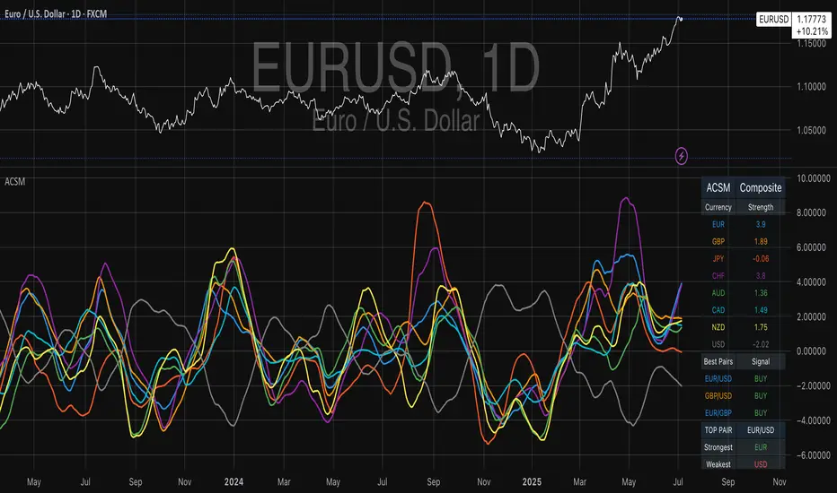
Intrinsic Event (Multi DC OS)Overview
This indicator implements an event-based approach to analyze price movements in the foreign exchange market, inspired by the intrinsic time framework introduced in Fractals and Intrinsic Time - A Challenge to Econometricians by U. A. Müller et al. (1995). It identifies significant price events using an intrinsic time perspective and supports multi-agent analysis to reflect the heterogeneous nature of financial markets. The script plots these events as lines and labels on the chart, offering a visual tool for traders to understand market dynamics at different scales.
Key Features
Intrinsic Events : The indicator detects directional change (DC) and overshoot (OS) events based on user-defined thresholds (delta), aligning with the paper’s concept of intrinsic time (Section 6). Intrinsic time redefines time based on market activity, expanding during volatile periods and contracting during inactive ones, rather than relying on a physical clock.
Multi-Agent Analysis : Supports up to five agents, each with its own threshold and color settings, reflecting the heterogeneous market hypothesis (Section 5). This allows the indicator to capture the perspectives of market participants with different time horizons, such as short-term FX dealers and long-term central banks.
How It Works
Intrinsic Events Detection : The script identifies two types of events using intrinsic time principles:
Directional Change (DC) : Triggered when the price reverses by the threshold (delta) against the current trend (e.g., a drop by delta in an uptrend signals a "Down DC").
Overshoot (OS) : Occurs when the price continues in the trend direction by the threshold (e.g., a rise by delta in an uptrend signals an "Up OS").
DC events are plotted as solid lines, and OS events as dashed lines, with labels like "Up DC" or "OS Down" for clarity. The label style adjusts based on the trend to ensure visibility.
Multi-Agent Setup : Each agent operates independently with its own threshold, mimicking market participants with varying time horizons (Section 5). Smaller thresholds detect frequent, short-term events, while larger thresholds capture broader, long-term movements.
Settings
Each agent can be configured with:
Enable Agent : Toggle the agent on or off.
Threshold (%) : The percentage threshold (delta) for detecting DC and OS events (default values: 0.1%, 0.2%, 0.5%, 1%, 2% for agents 1–5).
Up Mode Color : Color for lines and labels in up mode (DC events).
Down Mode Color : Color for lines and labels in down mode (OS events).
Usage Notes
This indicator is designed for the foreign exchange market, leveraging its high liquidity, as noted in the paper (Section 1). Adjust the threshold values based on the instrument’s volatility—higher volatility leads to more intrinsic events (Section 4). It can be adapted to other markets where event-based analysis applies.
Reference
The methodology is based on:
Fractals and Intrinsic Time - A Challenge to Econometricians by U. A. Müller, M. M. Dacorogna, R. D. Davé, O. V. Pictet, R. B. Olsen, and J. R. Ward (June 28, 1995). Olsen & Associates Preprint.

Black Scholes Option Pricing Model w/ Greeks [Loxx]The Black Scholes Merton model
If you are new to options I strongly advise you to profit from Robert Shiller's lecture on same . It combines practical market insights with a strong authoritative grasp of key models in option theory. He explains many of the areas covered below and in the following pages with a lot intuition and relatable anecdotage. We start here with Black Scholes Merton which is probably the most popular option pricing framework, due largely to its simplicity and ease in terms of implementation. The closed-form solution is efficient in terms of speed and always compares favorably relative to any numerical technique. The Black–Scholes–Merton model is a mathematical go-to model for estimating the value of European calls and puts. In the early 1970’s, Myron Scholes, and Fisher Black made an important breakthrough in the pricing of complex financial instruments. Robert Merton simultaneously was working on the same problem and applied the term Black-Scholes model to describe new generation of pricing. The Black Scholes (1973) contribution developed insights originally proposed by Bachelier 70 years before. In 1997, Myron Scholes and Robert Merton received the Nobel Prize for Economics. Tragically, Fisher Black died in 1995. The Black–Scholes formula presents a theoretical estimate (or model estimate) of the price of European-style options independently of the risk of the underlying security. Future payoffs from options can be discounted using the risk-neutral rate. Earlier academic work on options (e.g., Malkiel and Quandt 1968, 1969) had contemplated using either empirical, econometric analyses or elaborate theoretical models that possessed parameters whose values could not be calibrated directly. In contrast, Black, Scholes, and Merton’s parameters were at their core simple and did not involve references to utility or to the shifting risk appetite of investors. Below, we present a standard type formula, where: c = Call option value, p = Put option value, S=Current stock (or other underlying) price, K or X=Strike price, r=Risk-free interest rate, q = dividend yield, T=Time to maturity and N denotes taking the normal cumulative probability. b = (r - q) = cost of carry. (via VinegarHill-Financelab )
Things to know
This can only be used on the daily timeframe
You must select the option type and the greeks you wish to show
This indicator is a work in process, functions may be updated in the future. I will also be adding additional greeks as I code them or they become available in finance literature. This indictor contains 18 greeks. Many more will be added later.
Inputs
Spot price: select from 33 different types of price inputs
Calculation Steps: how many iterations to be used in the BS model. In practice, this number would be anywhere from 5000 to 15000, for our purposes here, this is limited to 300
Strike Price: the strike price of the option you're wishing to model
% Implied Volatility: here you can manually enter implied volatility
Historical Volatility Period: the input period for historical volatility ; historical volatility isn't used in the BS process, this is to serve as a sort of benchmark for the implied volatility ,
Historical Volatility Type: choose from various types of implied volatility , search my indicators for details on each of these
Option Base Currency: this is to calculate the risk-free rate, this is used if you wish to automatically calculate the risk-free rate instead of using the manual input. this uses the 10 year bold yield of the corresponding country
% Manual Risk-free Rate: here you can manually enter the risk-free rate
Use manual input for Risk-free Rate? : choose manual or automatic for risk-free rate
% Manual Yearly Dividend Yield: here you can manually enter the yearly dividend yield
Adjust for Dividends?: choose if you even want to use use dividends
Automatically Calculate Yearly Dividend Yield? choose if you want to use automatic vs manual dividend yield calculation
Time Now Type: choose how you want to calculate time right now, see the tool tip
Days in Year: choose how many days in the year, 365 for all days, 252 for trading days, etc
Hours Per Day: how many hours per day? 24, 8 working hours, or 6.5 trading hours
Expiry date settings: here you can specify the exact time the option expires
The Black Scholes Greeks
The Option Greek formulae express the change in the option price with respect to a parameter change taking as fixed all the other inputs. ( Haug explores multiple parameter changes at once .) One significant use of Greek measures is to calibrate risk exposure. A market-making financial institution with a portfolio of options, for instance, would want a snap shot of its exposure to asset price, interest rates, dividend fluctuations. It would try to establish impacts of volatility and time decay. In the formulae below, the Greeks merely evaluate change to only one input at a time. In reality, we might expect a conflagration of changes in interest rates and stock prices etc. (via VigengarHill-Financelab )
First-order Greeks
Delta: Delta measures the rate of change of the theoretical option value with respect to changes in the underlying asset's price. Delta is the first derivative of the value
Vega: Vegameasures sensitivity to volatility. Vega is the derivative of the option value with respect to the volatility of the underlying asset.
Theta: Theta measures the sensitivity of the value of the derivative to the passage of time (see Option time value): the "time decay."
Rho: Rho measures sensitivity to the interest rate: it is the derivative of the option value with respect to the risk free interest rate (for the relevant outstanding term).
Lambda: Lambda, Omega, or elasticity is the percentage change in option value per percentage change in the underlying price, a measure of leverage, sometimes called gearing.
Epsilon: Epsilon, also known as psi, is the percentage change in option value per percentage change in the underlying dividend yield, a measure of the dividend risk. The dividend yield impact is in practice determined using a 10% increase in those yields. Obviously, this sensitivity can only be applied to derivative instruments of equity products.
Second-order Greeks
Gamma: Measures the rate of change in the delta with respect to changes in the underlying price. Gamma is the second derivative of the value function with respect to the underlying price.
Vanna: Vanna, also referred to as DvegaDspot and DdeltaDvol, is a second order derivative of the option value, once to the underlying spot price and once to volatility. It is mathematically equivalent to DdeltaDvol, the sensitivity of the option delta with respect to change in volatility; or alternatively, the partial of vega with respect to the underlying instrument's price. Vanna can be a useful sensitivity to monitor when maintaining a delta- or vega-hedged portfolio as vanna will help the trader to anticipate changes to the effectiveness of a delta-hedge as volatility changes or the effectiveness of a vega-hedge against change in the underlying spot price.
Charm: Charm or delta decay measures the instantaneous rate of change of delta over the passage of time.
Vomma: Vomma, volga, vega convexity, or DvegaDvol measures second order sensitivity to volatility. Vomma is the second derivative of the option value with respect to the volatility, or, stated another way, vomma measures the rate of change to vega as volatility changes.
Veta: Veta or DvegaDtime measures the rate of change in the vega with respect to the passage of time. Veta is the second derivative of the value function; once to volatility and once to time.
Vera: Vera (sometimes rhova) measures the rate of change in rho with respect to volatility. Vera is the second derivative of the value function; once to volatility and once to interest rate.
Third-order Greeks
Speed: Speed measures the rate of change in Gamma with respect to changes in the underlying price.
Zomma: Zomma measures the rate of change of gamma with respect to changes in volatility.
Color: Color, gamma decay or DgammaDtime measures the rate of change of gamma over the passage of time.
Ultima: Ultima measures the sensitivity of the option vomma with respect to change in volatility.
Dual Delta: Dual Delta determines how the option price changes in relation to the change in the option strike price; it is the first derivative of the option price relative to the option strike price
Dual Gamma: Dual Gamma determines by how much the coefficient will changedual delta when the option strike price changes; it is the second derivative of the option price relative to the option strike price.
Related Indicators
Cox-Ross-Rubinstein Binomial Tree Options Pricing Model
Implied Volatility Estimator using Black Scholes
Boyle Trinomial Options Pricing Model
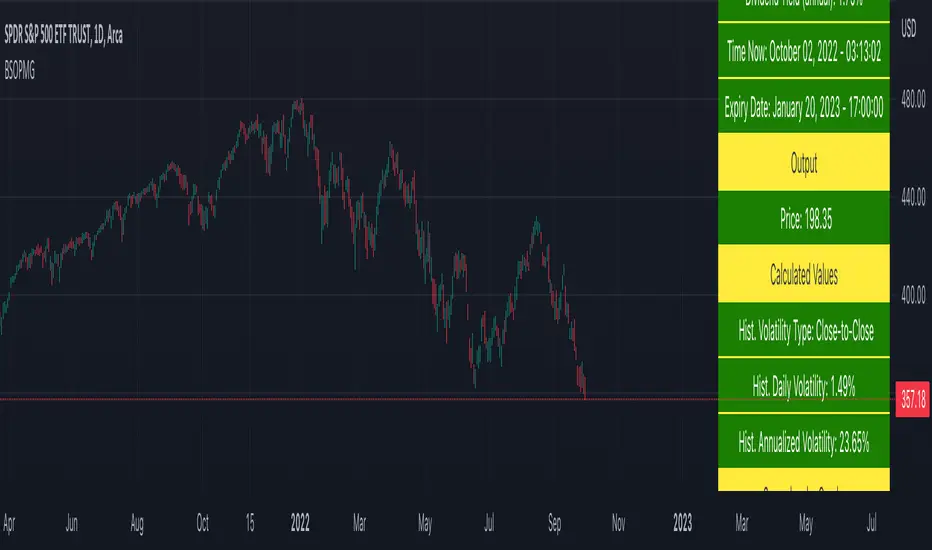
Connors-Hayward Advance-Decline Trading PatternsThe following is an excerpt from Investment Secrets of a Hedge Fund Manager
"The Connors-Hayward Advance-Decline Trading Pattern (CHADTP) is a proprietary indicator we use to identify short- and intermediate-term overbought and oversold conditions for the stock market and the S&P 500 futures market...
Construction of the CHADTP indicator is simple:
Add the past five day's advancing issues from the New York Stock Exchange.
Add the past five day's declining issues from the NYSE.
Subtract #2 from #1.
Divide by five.
Here are the two rules to trade CHADTP:
When the five-day reading is above +400, the market is overbought; and when the five day reading is below -400, the market is oversold.
Unfortunately, just because the indicator is -400 does not mean we can blindly buy the market, and just because the indicator is +400 does not mean we should be a seller of the market.
Whenever we get an overbought or oversold reading, we wait for a specific price reversal before entering. When the CHADTP number is +400 or more, we will sell the market only after the S&P 500 futures trade .10 points below the previous day's low. For example, if we get a reading of +422 and today's low is 453.80 we will take a sell signal only if the market trades at 453.70 or below tomorrow. If tomorrow the market low is 454.60, and the CHADTP is above 400, we will only sell if the market trades at 454.50 or below the next day, and so on. On the buy side, if today's CHADTP number is -400 or less, we will buy only after tomorrow's S&P trades .10 points above today's high, and so on."
Note from Technicus Capital:
This method was created in 1995. Today, the volume and volatility of markets is much more significant and therefore the original overbought/oversold levels are no longer relevant.
TimeSeriesBenchmarkMeasuresLibrary "TimeSeriesBenchmarkMeasures"
Time Series Benchmark Metrics. \
Provides a comprehensive set of functions for benchmarking time series data, allowing you to evaluate the accuracy, stability, and risk characteristics of various models or strategies. The functions cover a wide range of statistical measures, including accuracy metrics (MAE, MSE, RMSE, NRMSE, MAPE, SMAPE), autocorrelation analysis (ACF, ADF), and risk measures (Theils Inequality, Sharpness, Resolution, Coverage, and Pinball).
___
Reference:
- github.com .
- medium.com .
- www.salesforce.com .
- towardsdatascience.com .
- github.com .
mae(actual, forecasts)
In statistics, mean absolute error (MAE) is a measure of errors between paired observations expressing the same phenomenon. Examples of Y versus X include comparisons of predicted versus observed, subsequent time versus initial time, and one technique of measurement versus an alternative technique of measurement.
Parameters:
actual (array) : List of actual values.
forecasts (array) : List of forecasts values.
Returns: - Mean Absolute Error (MAE).
___
Reference:
- en.wikipedia.org .
- The Orange Book of Machine Learning - Carl McBride Ellis .
mse(actual, forecasts)
The Mean Squared Error (MSE) is a measure of the quality of an estimator. As it is derived from the square of Euclidean distance, it is always a positive value that decreases as the error approaches zero.
Parameters:
actual (array) : List of actual values.
forecasts (array) : List of forecasts values.
Returns: - Mean Squared Error (MSE).
___
Reference:
- en.wikipedia.org .
rmse(targets, forecasts, order, offset)
Calculates the Root Mean Squared Error (RMSE) between target observations and forecasts. RMSE is a standard measure of the differences between values predicted by a model and the values actually observed.
Parameters:
targets (array) : List of target observations.
forecasts (array) : List of forecasts.
order (int) : Model order parameter that determines the starting position in the targets array, `default=0`.
offset (int) : Forecast offset related to target, `default=0`.
Returns: - RMSE value.
nmrse(targets, forecasts, order, offset)
Normalised Root Mean Squared Error.
Parameters:
targets (array) : List of target observations.
forecasts (array) : List of forecasts.
order (int) : Model order parameter that determines the starting position in the targets array, `default=0`.
offset (int) : Forecast offset related to target, `default=0`.
Returns: - NRMSE value.
rmse_interval(targets, forecasts)
Root Mean Squared Error for a set of interval windows. Computes RMSE by converting interval forecasts (with min/max bounds) into point forecasts using the mean of the interval bounds, then compares against actual target values.
Parameters:
targets (array) : List of target observations.
forecasts (matrix) : The forecasted values in matrix format with at least 2 columns (min, max).
Returns: - RMSE value for the combined interval list.
mape(targets, forecasts)
Mean Average Percentual Error.
Parameters:
targets (array) : List of target observations.
forecasts (array) : List of forecasts.
Returns: - MAPE value.
smape(targets, forecasts, mode)
Symmetric Mean Average Percentual Error. Calculates the Mean Absolute Percentage Error (MAPE) between actual targets and forecasts. MAPE is a common metric for evaluating forecast accuracy, expressed as a percentage, lower values indicate a better forecast accuracy.
Parameters:
targets (array) : List of target observations.
forecasts (array) : List of forecasts.
mode (int) : Type of method: default=0:`sum(abs(Fi-Ti)) / sum(Fi+Ti)` , 1:`mean(abs(Fi-Ti) / ((Fi + Ti) / 2))` , 2:`mean(abs(Fi-Ti) / (abs(Fi) + abs(Ti))) * 100`
Returns: - SMAPE value.
mape_interval(targets, forecasts)
Mean Average Percentual Error for a set of interval windows.
Parameters:
targets (array) : List of target observations.
forecasts (matrix) : The forecasted values in matrix format with at least 2 columns (min, max).
Returns: - MAPE value for the combined interval list.
acf(data, k)
Autocorrelation Function (ACF) for a time series at a specified lag.
Parameters:
data (array) : Sample data of the observations.
k (int) : The lag period for which to calculate the autocorrelation. Must be a non-negative integer.
Returns: - The autocorrelation value at the specified lag, ranging from -1 to 1.
___
The autocorrelation function measures the linear dependence between observations in a time series
at different time lags. It quantifies how well the series correlates with itself at different
time intervals, which is useful for identifying patterns, seasonality, and the appropriate
lag structure for time series models.
ACF values close to 1 indicate strong positive correlation, values close to -1 indicate
strong negative correlation, and values near 0 indicate no linear correlation.
___
Reference:
- statisticsbyjim.com
acf_multiple(data, k)
Autocorrelation function (ACF) for a time series at a set of specified lags.
Parameters:
data (array) : Sample data of the observations.
k (array) : List of lag periods for which to calculate the autocorrelation. Must be a non-negative integer.
Returns: - List of ACF values for provided lags.
___
The autocorrelation function measures the linear dependence between observations in a time series
at different time lags. It quantifies how well the series correlates with itself at different
time intervals, which is useful for identifying patterns, seasonality, and the appropriate
lag structure for time series models.
ACF values close to 1 indicate strong positive correlation, values close to -1 indicate
strong negative correlation, and values near 0 indicate no linear correlation.
___
Reference:
- statisticsbyjim.com
adfuller(data, n_lag, conf)
: Augmented Dickey-Fuller test for stationarity.
Parameters:
data (array) : Data series.
n_lag (int) : Maximum lag.
conf (string) : Confidence Probability level used to test for critical value, (`90%`, `95%`, `99%`).
Returns: - `adf` The test statistic.
- `crit` Critical value for the test statistic at the 10 % levels.
- `nobs` Number of observations used for the ADF regression and calculation of the critical values.
___
The Augmented Dickey-Fuller test is used to determine whether a time series is stationary
or contains a unit root (non-stationary). The null hypothesis is that the series has a unit root
(is non-stationary), while the alternative hypothesis is that the series is stationary.
A stationary time series has statistical properties that do not change over time, making it
suitable for many time series forecasting models. If the test statistic is less than the
critical value, we reject the null hypothesis and conclude the series is stationary.
___
Reference:
- www.jstor.org
- en.wikipedia.org
theils_inequality(targets, forecasts)
Calculates Theil's Inequality Coefficient, a measure of forecast accuracy that quantifies the relative difference between actual and predicted values.
Parameters:
targets (array) : List of target observations.
forecasts (array) : Matrix with list of forecasts, ordered column wise.
Returns: - Theil's Inequality Coefficient value, value closer to 0 is better.
___
Theil's Inequality Coefficient is calculated as: `sqrt(Sum((y_i - f_i)^2)) / (sqrt(Sum(y_i^2)) + sqrt(Sum(f_i^2)))`
where `y_i` represents actual values and `f_i` represents forecast values.
This metric ranges from 0 to infinity, with 0 indicating perfect forecast accuracy.
___
Reference:
- en.wikipedia.org
sharpness(forecasts)
The average width of the forecast intervals across all observations, representing the sharpness or precision of the predictive intervals.
Parameters:
forecasts (matrix) : The forecasted values in matrix format with at least 2 columns (min, max).
Returns: - Sharpness The sharpness level, which is the average width of all prediction intervals across the forecast horizon.
___
Sharpness is an important metric for evaluating forecast quality. It measures how narrow or wide the
prediction intervals are. Higher sharpness (narrower intervals) indicates greater precision in the
forecast intervals, while lower sharpness (wider intervals) suggests less precision.
The sharpness metric is calculated as the mean of the interval widths across all observations, where
each interval width is the difference between the upper and lower bounds of the prediction interval.
Note: This function assumes that the forecasts matrix has at least 2 columns, with the first column
representing the lower bounds and the second column representing the upper bounds of prediction intervals.
___
Reference:
- Hyndman, R. J., & Athanasopoulos, G. (2018). Forecasting: principles and practice. OTexts. otexts.com
resolution(forecasts)
Calculates the resolution of forecast intervals, measuring the average absolute difference between individual forecast interval widths and the overall sharpness measure.
Parameters:
forecasts (matrix) : The forecasted values in matrix format with at least 2 columns (min, max).
Returns: - The average absolute difference between individual forecast interval widths and the overall sharpness measure, representing the resolution of the forecasts.
___
Resolution is a key metric for evaluating forecast quality that measures the consistency of prediction
interval widths. It quantifies how much the individual forecast intervals vary from the average interval
width (sharpness). High resolution indicates that the forecast intervals are relatively consistent
across observations, while low resolution suggests significant variation in interval widths.
The resolution is calculated as the mean absolute deviation of individual interval widths from the
overall sharpness value. This provides insight into the uniformity of the forecast uncertainty
estimates across the forecast horizon.
Note: This function requires the forecasts matrix to have at least 2 columns (min, max) representing
the lower and upper bounds of prediction intervals.
___
Reference:
- (sites.stat.washington.edu)
- (www.jstor.org)
coverage(targets, forecasts)
Calculates the coverage probability, which is the percentage of target values that fall within the corresponding forecasted prediction intervals.
Parameters:
targets (array) : List of target values.
forecasts (matrix) : The forecasted values in matrix format with at least 2 columns (min, max).
Returns: - Percent of target values that fall within their corresponding forecast intervals, expressed as a decimal value between 0 and 1 (or 0% and 100%).
___
Coverage probability is a crucial metric for evaluating the reliability of prediction intervals.
It measures how well the forecast intervals capture the actual observed values. An ideal forecast
should have a coverage probability close to the nominal confidence level (e.g., 90%, 95%, or 99%).
For example, if a 95% prediction interval is used, we expect approximately 95% of the actual
target values to fall within those intervals. If the coverage is significantly lower than the
nominal level, the intervals may be too narrow; if it's significantly higher, the intervals may
be too wide.
Note: This function requires the targets array and forecasts matrix to have the same number of
observations, and the forecasts matrix must have at least 2 columns (min, max) representing
the lower and upper bounds of prediction intervals.
___
Reference:
- (www.jstor.org)
pinball(tau, target, forecast)
Pinball loss function, measures the asymmetric loss for quantile forecasts.
Parameters:
tau (float) : The quantile level (between 0 and 1), where 0.5 represents the median.
target (float) : The actual observed value to compare against.
forecast (float) : The forecasted value.
Returns: - The Pinball loss value, which quantifies the distance between the forecast and target relative to the specified quantile level.
___
The Pinball loss function is specifically designed for evaluating quantile forecasts. It is
asymmetric, meaning it penalizes underestimates and overestimates differently depending on the
quantile level being evaluated.
For a given quantile τ, the loss function is defined as:
- If target >= forecast: (target - forecast) * τ
- If target < forecast: (forecast - target) * (1 - τ)
This loss function is commonly used in quantile regression and probabilistic forecasting
to evaluate how well forecasts capture specific quantiles of the target distribution.
___
Reference:
- (www.otexts.com)
pinball_mean(tau, targets, forecasts)
Calculates the mean pinball loss for quantile regression.
Parameters:
tau (float) : The quantile level (between 0 and 1), where 0.5 represents the median.
targets (array) : The actual observed values to compare against.
forecasts (matrix) : The forecasted values in matrix format with at least 2 columns (min, max).
Returns: - The mean pinball loss value across all observations.
___
The pinball_mean() function computes the average Pinball loss across multiple observations,
making it suitable for evaluating overall forecast performance in quantile regression tasks.
This function leverages the asymmetric Pinball loss function to evaluate how well forecasts
capture specific quantiles of the target distribution. The choice of which column from the
forecasts matrix to use depends on the quantile level:
- For τ ≤ 0.5: Uses the first column (min) of forecasts
- For τ > 0.5: Uses the second column (max) of forecasts
This loss function is commonly used in quantile regression and probabilistic forecasting
to evaluate how well forecasts capture specific quantiles of the target distribution.
___
Reference:
- (www.otexts.com)
Triple Exponential Moving Average (TEMA)The Triple Exponential Moving Average (TEMA) is an advanced technical indicator designed to significantly reduce the lag inherent in traditional moving averages while maintaining signal quality. Developed by Patrick Mulloy in 1994 as an extension of his DEMA concept, TEMA employs a sophisticated triple-stage calculation process to provide exceptionally responsive market signals.
TEMA's mathematical approach goes beyond standard smoothing techniques by using a triple-cascade architecture with optimized coefficients. This makes it particularly valuable for traders who need earlier identification of trend changes without sacrificing reliability. Since its introduction, TEMA has become a key component in many algorithmic trading systems and professional trading platforms.
▶️ **Core Concepts**
Triple-stage lag reduction: TEMA uses a three-level EMA calculation with optimized coefficients (3, -3, 1) to dramatically minimize the delay in signal generation
Enhanced responsiveness: Provides significantly faster reaction to price changes than standard EMA or even DEMA, while maintaining reasonable smoothness
Strategic signal processing: Employs mathematical techniques to extract the underlying trend while filtering random price fluctuations
Timeframe effectiveness: Performs well across multiple timeframes, though particularly valued in short to medium-term trading
TEMA achieves its enhanced responsiveness through an innovative triple-cascade architecture that strategically combines three levels of exponential moving averages. This approach effectively removes the lag component inherent in EMA calculations while preserving the essential smoothing benefits.
▶️ **Common Settings and Parameters**
Length: Default: 12 | Controls sensitivity/smoothness | When to Adjust: Increase in choppy markets, decrease in strongly trending markets
Source: Default: Close | Data point used for calculation | When to Adjust: Change to HL2/HLC3 for more balanced price representation
Corrected: Default: false | Adjusts internal EMA smoothing factors for potentially faster response | When to Adjust: Set to true for a modified TEMA that may react quicker to price changes. false uses standard TEMA calculation
Visualization: Default: Line | Display format on charts | When to Adjust: Use filled cloud to see divergence from price more clearly
Pro Tip: For optimal trade signals, many professional traders use two TEMAs (e.g., 8 and 21 periods) and look for crossovers, which often provide earlier signals than traditional moving average pairs.
▶️ **Calculation and Mathematical Foundation**
Simplified explanation:
TEMA calculates three levels of EMAs, then combines them using a special formula that amplifies recent price action while reducing lag. This triple-processing approach effectively eliminates much of the delay found in traditional moving averages.
Technical formula:
TEMA = 3 × EMA₁ - 3 × EMA₂ + EMA₃
Where:
EMA₁ = EMA(source, α₁)
EMA₂ = EMA(EMA₁, α₂)
EMA₃ = EMA(EMA₂, α₃)
The smoothing factors (α₁, α₂, α₃) are determined as follows:
Let α_base = 2/(length + 1)
α₁ = α_base
If corrected is false:
α₂ = α_base
α₃ = α_base
If corrected is true:
Let r = (1/α_base)^(1/3)
α₂ = α_base * r
α₃ = α_base * r * r = α_base * r²
The corrected = true option implements a variation that uses progressively smaller alpha values for the subsequent EMA calculations. This approach aims to optimize the filter's frequency response and phase lag.
Alpha Calculation for corrected = true:
α₁ (alpha_base) = 2/(length + 1)
r = (1/α₁)^(1/3) (cube root relationship)
α₂ = α₁ * r = α₁^(2/3)
α₃ = α₂ * r = α₁^(1/3)
Mathematical Rationale for Corrected Alphas:
1. Frequency Response Balance:
The standard TEMA (where α₁ = α₂ = α₃) can lead to an uneven frequency response, potentially over-smoothing high frequencies or creating resonance artifacts. The geometric progression of alphas (α₁ > α₁^(2/3) > α₁^(1/3)) in the corrected version aims to create a more balanced filter cascade. Each stage contributes more proportionally to the overall frequency response.
2. Phase Lag Optimization:
The cube root relationship between the alphas is designed to minimize cumulative phase lag while maintaining smoothing effectiveness. Each subsequent EMA stage has a progressively smaller impact on phase distortion.
3. Mathematical Stability:
The geometric progression (α₁, α₁^(2/3), α₁^(1/3)) can enhance numerical stability due to constant ratios between consecutive alphas. This helps prevent the accumulation of rounding errors and maintains consistent convergence properties.
Practical Impact of corrected = true:
This modification aims to achieve:
Potentially better lag reduction for a similar level of smoothing
A more uniform frequency response across different market cycles
Reduced overshoot or undershoot in trending conditions
Improved signal-to-noise ratio preservation
Essentially, the cube root relationship in the corrected TEMA attempts to optimize the trade-off between responsiveness and smoothness that can be a challenge with uniform alpha values.
🔍 Technical Note: Advanced implementations apply compensation techniques to all three EMA stages, ensuring TEMA values are valid from the first bar without requiring a warm-up period. This compensation corrects initialization bias and prevents calculation errors from compounding through the cascade.
▶️ **Interpretation Details**
TEMA excels at identifying trend changes significantly earlier than traditional moving averages, making it valuable for both entry and exit signals:
When price crosses above TEMA, it often signals the beginning of an uptrend
When price crosses below TEMA, it often signals the beginning of a downtrend
The slope of TEMA provides insight into trend strength and momentum
TEMA crossovers with price tend to occur earlier than with standard EMAs
When multiple-period TEMAs cross each other, they confirm significant trend shifts
TEMA works exceptionally well as a dynamic support/resistance level in trending markets
For optimal results, traders often use TEMA in combination with momentum indicators or volume analysis to confirm signals and reduce false positives.
▶️ **Limitations and Considerations**
Market conditions: The high responsiveness can generate false signals during highly choppy, sideways markets
Overshooting: More aggressive lag reduction leads to more pronounced overshooting during sharp reversals
Parameter sensitivity: Changes in length have more dramatic effects than in simpler moving averages
Calculation complexity: Triple cascaded EMAs make behavior less predictable and more resource-intensive
Complementary tools: Should be used with confirmation tools like RSI, MACD or volume indicators
▶️ **References**
Mulloy, P. (1994). "Smoothing Data with Less Lag," Technical Analysis of Stocks & Commodities .
Mulloy, P. (1995). "Comparing Digital Filters," Technical Analysis of Stocks & Commodities .
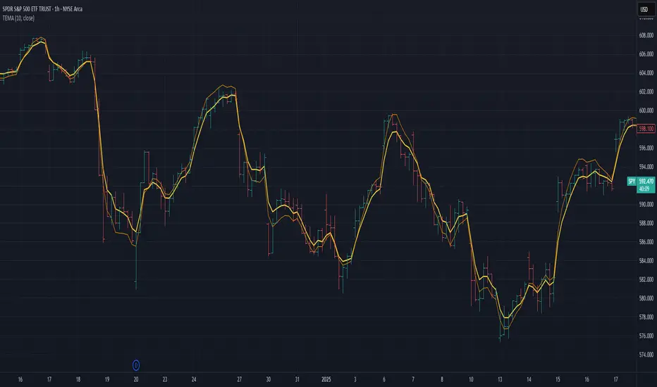
Goldman Sachs Risk Appetite ProxyRisk appetite indicators serve as barometers of market psychology, measuring investors' collective willingness to engage in risk-taking behavior. According to Mosley & Singer (2008), "cross-asset risk sentiment indicators provide valuable leading signals for market direction by capturing the underlying psychological state of market participants before it fully manifests in price action."
The GSRAI methodology aligns with modern portfolio theory, which emphasizes the importance of cross-asset correlations during different market regimes. As noted by Ang & Bekaert (2002), "asset correlations tend to increase during market stress, exhibiting asymmetric patterns that can be captured through multi-asset sentiment indicators."
Implementation Methodology
Component Selection
Our implementation follows the core framework outlined by Goldman Sachs research, focusing on four key components:
Credit Spreads (High Yield Credit Spread)
As noted by Duca et al. (2016), "credit spreads provide a market-based assessment of default risk and function as an effective barometer of economic uncertainty." Higher spreads generally indicate deteriorating risk appetite.
Volatility Measures (VIX)
Baker & Wurgler (2006) established that "implied volatility serves as a direct measure of market fear and uncertainty." The VIX, often called the "fear gauge," maintains an inverse relationship with risk appetite.
Equity/Bond Performance Ratio (SPY/IEF)
According to Connolly et al. (2005), "the relative performance of stocks versus bonds offers significant insight into market participants' risk preferences and flight-to-safety behavior."
Commodity Ratio (Oil/Gold)
Baur & McDermott (2010) demonstrated that "gold often functions as a safe haven during market turbulence, while oil typically performs better during risk-on environments, making their ratio an effective risk sentiment indicator."
Standardization Process
Each component undergoes z-score normalization to enable cross-asset comparisons, following the statistical approach advocated by Burdekin & Siklos (2012). The z-score transformation standardizes each variable by subtracting its mean and dividing by its standard deviation: Z = (X - μ) / σ
This approach allows for meaningful aggregation of different market signals regardless of their native scales or volatility characteristics.
Signal Integration
The four standardized components are equally weighted and combined to form a composite score. This democratic weighting approach is supported by Rapach et al. (2010), who found that "simple averaging often outperforms more complex weighting schemes in financial applications due to estimation error in the optimization process."
The final index is scaled to a 0-100 range, with:
Values above 70 indicating "Risk-On" market conditions
Values below 30 indicating "Risk-Off" market conditions
Values between 30-70 representing neutral risk sentiment
Limitations and Differences from Original Implementation
Proprietary Components
The original Goldman Sachs indicator incorporates additional proprietary elements not publicly disclosed. As Goldman Sachs Global Investment Research (2019) notes, "our comprehensive risk appetite framework incorporates proprietary positioning data and internal liquidity metrics that enhance predictive capability."
Technical Limitations
Pine Script v6 imposes certain constraints that prevent full replication:
Structural Limitations: Functions like plot, hline, and bgcolor must be defined in the global scope rather than conditionally, requiring workarounds for dynamic visualization.
Statistical Processing: Advanced statistical methods used in the original model, such as Kalman filtering or regime-switching models described by Ang & Timmermann (2012), cannot be fully implemented within Pine Script's constraints.
Data Availability: As noted by Kilian & Park (2009), "the quality and frequency of market data significantly impacts the effectiveness of sentiment indicators." Our implementation relies on publicly available data sources that may differ from Goldman Sachs' institutional data feeds.
Empirical Performance
While a formal backtest comparison with the original GSRAI is beyond the scope of this implementation, research by Froot & Ramadorai (2005) suggests that "publicly accessible proxies of proprietary sentiment indicators can capture a significant portion of their predictive power, particularly during major market turning points."
References
Ang, A., & Bekaert, G. (2002). "International Asset Allocation with Regime Shifts." Review of Financial Studies, 15(4), 1137-1187.
Ang, A., & Timmermann, A. (2012). "Regime Changes and Financial Markets." Annual Review of Financial Economics, 4(1), 313-337.
Baker, M., & Wurgler, J. (2006). "Investor Sentiment and the Cross-Section of Stock Returns." Journal of Finance, 61(4), 1645-1680.
Baur, D. G., & McDermott, T. K. (2010). "Is Gold a Safe Haven? International Evidence." Journal of Banking & Finance, 34(8), 1886-1898.
Burdekin, R. C., & Siklos, P. L. (2012). "Enter the Dragon: Interactions between Chinese, US and Asia-Pacific Equity Markets, 1995-2010." Pacific-Basin Finance Journal, 20(3), 521-541.
Connolly, R., Stivers, C., & Sun, L. (2005). "Stock Market Uncertainty and the Stock-Bond Return Relation." Journal of Financial and Quantitative Analysis, 40(1), 161-194.
Duca, M. L., Nicoletti, G., & Martinez, A. V. (2016). "Global Corporate Bond Issuance: What Role for US Quantitative Easing?" Journal of International Money and Finance, 60, 114-150.
Froot, K. A., & Ramadorai, T. (2005). "Currency Returns, Intrinsic Value, and Institutional-Investor Flows." Journal of Finance, 60(3), 1535-1566.
Goldman Sachs Global Investment Research (2019). "Risk Appetite Framework: A Practitioner's Guide."
Kilian, L., & Park, C. (2009). "The Impact of Oil Price Shocks on the U.S. Stock Market." International Economic Review, 50(4), 1267-1287.
Mosley, L., & Singer, D. A. (2008). "Taking Stock Seriously: Equity Market Performance, Government Policy, and Financial Globalization." International Studies Quarterly, 52(2), 405-425.
Oppenheimer, P. (2007). "A Framework for Financial Market Risk Appetite." Goldman Sachs Global Economics Paper.
Rapach, D. E., Strauss, J. K., & Zhou, G. (2010). "Out-of-Sample Equity Premium Prediction: Combination Forecasts and Links to the Real Economy." Review of Financial Studies, 23(2), 821-862.
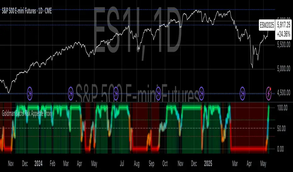
Interest Rate Trading (Manually Added Rate Decisions) [TANHEF]Interest Rate Trading: How Interest Rates Can Guide Your Next Move.
How were interest rate decisions added?
All interest rate decision dates were manually retrieved from the 'Record of Policy Actions' and 'Minutes of Actions' on the Federal Reserve's website due to inconsistent dates from other sources. These were manually added as Pine Script currently only identifies rate changes, not pauses.
█ Simple Explanation:
This script is designed for analyzing and backtesting trading strategies based on U.S. interest rate decisions which occur during Federal Open Market Committee (FOMC) meetings, to make trading decisions. No trading strategy is perfect, and it's important to understand that expectations won't always play out. The script leverages historical interest rate changes, including increases, decreases, and pauses, across multiple economic time periods from 1971 to the present. The tool integrates two key data sources for interest rates—USINTR and FEDFUNDS—to support decision-making around rate-based trades. The focus is on identifying opportunities and tracking trades driven by interest rate movements.
█ Interest Rate Decision Sources:
As noted above, each decision date has been manually added from the 'Record of Policy Actions' and 'Minutes of Actions' documents on the Federal Reserve's website. This includes +50 years of more than 600 rate decisions.
█ Interest Rate Data Sources:
USINTR: Reflects broader U.S. interest rate trends, including Treasury yields and various benchmarks. This is the preferred option as it corresponds well to the rate decision dates.
FEDFUNDS: Tracks the Federal Funds Rate, which is a more specific rate targeted by the Federal Reserve. This does not change on the exact same days as the rate decisions that occur at FOMC meetings.
█ Trade Criteria:
A variety of trading conditions are predefined to suit different trading strategies. These conditions include:
Increase/Decrease: Standard rate increases or decreases.
Double/Triple Increase/Decrease: A series of consecutive changes.
Aggressive Increase/Decrease: Rate changes that exceed recent movements.
Pause: Identification of no changes (pauses) between rate decisions, including double or triple pauses.
Complex Patterns: Combinations of pauses, increases, or decreases, such as "Pause after Increase" or "Pause or Increase."
█ Trade Execution and Exit:
The script allows automated trade execution based on selected criteria:
Auto-Entry: Option to enter trades automatically at the first valid period.
Max Trade Duration: Optional exit of trades after a specified number of bars (candles).
Pause Days: Minimum duration (in days) to validate rate pauses as entry conditions. This is especially useful for earlier periods (prior to the 2000s), where rate decisions often seemed random compared to the consistency we see today.
█ Visualization:
Several visual elements enhance the backtesting experience:
Time Period Highlighting: Economic time periods are visually segmented on the chart, each with a unique color. These periods include historical phases such as "Stagflation (1971-1982)" and "Post-Pandemic Recovery (2021-Present)".
Trade and Holding Results: Displays the profit and loss of trades and holding results directly on the chart.
Interest Rate Plot: Plots the interest rate movements on the chart, allowing for real-time tracking of rate changes.
Trade Status: Highlights active long or short positions on the chart.
█ Statistics and Criteria Display:
Stats Table: Summarizes trade results, including wins, losses, and draw percentages for both long and short trades.
Criteria Table: Lists the selected entry and exit criteria for both long and short positions.
█ Economic Time Periods:
The script organizes interest rate decisions into well-defined economic periods, allowing traders to backtest strategies specific to historical contexts like:
(1971-1982) Stagflation
(1983-1990) Reaganomics and Deregulation
(1991-1994) Early 1990s (Recession and Recovery)
(1995-2001) Dot-Com Bubble
(2001-2006) Housing Boom
(2007-2009) Global Financial Crisis
(2009-2015) Great Recession Recovery
(2015-2019) Normalization Period
(2019-2021) COVID-19 Pandemic
(2021-Present) Post-Pandemic Recovery
█ User-Configurable Inputs:
Rate Source Selection: Choose between USINTR or FEDFUNDS as the primary interest rate source.
Trade Criteria Customization: Users can select the criteria for long and short trades, specifying when to enter or exit based on changes in the interest rate.
Time Period: Select the time period that you want to isolate testing a strategy with.
Auto-Entry and Pause Settings: Options to automatically enter trades and specify the number of days to confirm a rate pause.
Max Trade Duration: Limits how long trades can remain open, defined by the number of bars.
█ Trade Logic:
The script manages entries and exits for both long and short trades. It calculates the profit or loss percentage based on the entry and exit prices. The script tracks ongoing trades, dynamically updating the profit or loss as price changes.
█ Examples:
One of the most popular opinions is that when rate starts begin you should sell, then buy back in when rate cuts stop dropping. However, this can be easily proven to be a difficult task. Predicting the end of a rate cut is very difficult to do with the the exception that assumes rates will not fall below 0.25%.
2001-2009
Trade Result: +29.85%
Holding Result: -27.74%
1971-2024
Trade Result: +533%
Holding Result: +5901%
█ Backtest and Real-Time Use:
This backtester is useful for historical analysis and real-time trading. By setting up various entry and exit rules tied to interest rate movements, traders can test and refine strategies based on real historical data and rate decision trends.
This powerful tool allows traders to customize strategies, backtest them through different economic periods, and get visual feedback on their trading performance, helping to make more informed decisions based on interest rate dynamics. The main goal of this indicator is to challenge the belief that future events must mirror the 2001 and 2007 rate cuts. If everyone expects something to happen, it usually doesn’t.
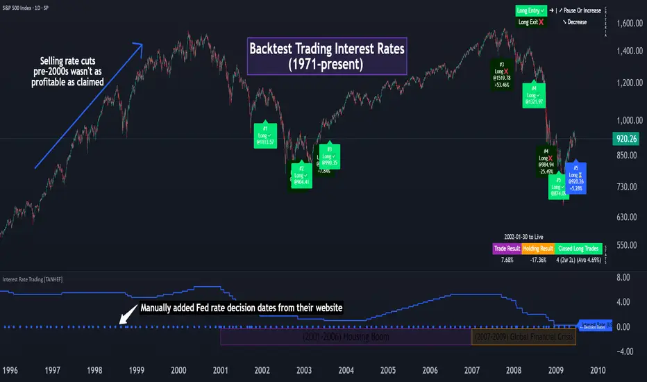
Larry Conners Vix Reversal II Strategy (approx.)This Pine Script™ strategy is a modified version of the original Larry Connors VIX Reversal II Strategy, designed for short-term trading in market indices like the S&P 500. The strategy utilizes the Relative Strength Index (RSI) of the VIX (Volatility Index) to identify potential overbought or oversold market conditions. The logic is based on the assumption that extreme levels of market volatility often precede reversals in price.
How the Strategy Works
The strategy calculates the RSI of the VIX using a 25-period lookback window. The RSI is a momentum oscillator that measures the speed and change of price movements. It ranges from 0 to 100 and is often used to identify overbought and oversold conditions in assets.
Overbought Signal: When the RSI of the VIX rises above 61, it signals a potential overbought condition in the market. The strategy looks for a RSI downtick (i.e., when RSI starts to fall after reaching this level) as a trigger to enter a long position.
Oversold Signal: Conversely, when the RSI of the VIX drops below 42, the market is considered oversold. A RSI uptick (i.e., when RSI starts to rise after hitting this level) serves as a signal to enter a short position.
The strategy holds the position for a minimum of 7 days and a maximum of 12 days, after which it exits automatically.
Larry Connors: Background
Larry Connors is a prominent figure in quantitative trading, specializing in short-term market strategies. He is the co-author of several influential books on trading, such as Street Smarts (1995), co-written with Linda Raschke, and How Markets Really Work. Connors' work focuses on developing rules-based systems using volatility indicators like the VIX and oscillators such as RSI to exploit mean-reversion patterns in financial markets.
Risks of the Strategy
While the Larry Connors VIX Reversal II Strategy can capture reversals in volatile market environments, it also carries significant risks:
Over-Optimization: This modified version adjusts RSI levels and holding periods to fit recent market data. If market conditions change, the strategy might no longer be effective, leading to false signals.
Drawdowns in Trending Markets: This is a mean-reversion strategy, designed to profit when markets return to a previous mean. However, in strongly trending markets, especially during extended bull or bear phases, the strategy might generate losses due to early entries or exits.
Volatility Risk: Since this strategy is linked to the VIX, an instrument that reflects market volatility, large spikes in volatility can lead to unexpected, fast-moving market conditions, potentially leading to larger-than-expected losses.
Scientific Literature and Supporting Research
The use of RSI and VIX in trading strategies has been widely discussed in academic research. RSI is one of the most studied momentum oscillators, and numerous studies show that it can capture mean-reversion effects in various markets, including equities and derivatives.
Wong et al. (2003) investigated the effectiveness of technical trading rules such as RSI, finding that it has predictive power in certain market conditions, particularly in mean-reverting markets .
The VIX, often referred to as the “fear index,” reflects market expectations of volatility and has been a focal point in research exploring volatility-based strategies. Whaley (2000) extensively reviewed the predictive power of VIX, noting that extreme VIX readings often correlate with turning points in the stock market .
Modified Version of Original Strategy
This script is a modified version of Larry Connors' original VIX Reversal II strategy. The key differences include:
Adjusted RSI period to 25 (instead of 2 or 4 commonly used in Connors’ other work).
Overbought and oversold levels modified to 61 and 42, respectively.
Specific holding period (7 to 12 days) is predefined to reduce holding risk.
These modifications aim to adapt the strategy to different market environments, potentially enhancing performance under specific volatility conditions. However, as with any system, constant evaluation and testing in live markets are crucial.
References
Wong, W. K., Manzur, M., & Chew, B. K. (2003). How rewarding is technical analysis? Evidence from Singapore stock market. Applied Financial Economics, 13(7), 543-551.
Whaley, R. E. (2000). The investor fear gauge. Journal of Portfolio Management, 26(3), 12-17.
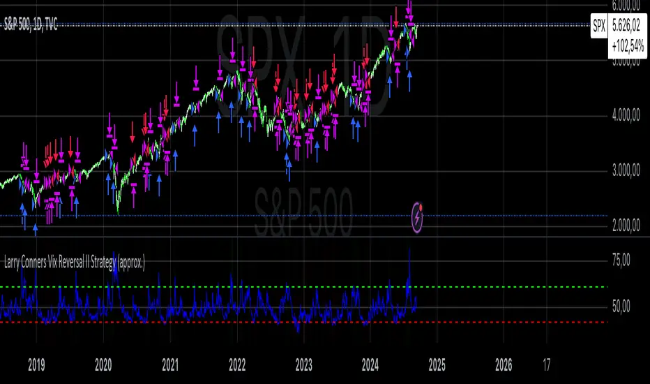
Larry Connors 3 Day High/Low StrategyThe Larry Connors 3 Day High/Low Strategy is a short-term mean-reversion trading strategy that is designed to identify potential buying opportunities when a security is oversold. This strategy is based on the principles developed by Larry Connors, a well-known trading system developer and author.
Key Strategy Elements:
1. Trend Confirmation: The strategy first confirms that the security is in a long-term uptrend by ensuring that the closing price is above the 200-day moving average (condition1). This rule helps filter trades to align with the longer-term trend.
2. Short-Term Pullback: The strategy looks for a short-term pullback by ensuring that the closing price is below the 5-day moving average (condition2). This identifies potential entry points when the price temporarily moves against the longer-term trend.
3. Three Consecutive Lower Highs and Lows:
• The high and low two days ago are lower than those of the day before (condition3).
• The high and low yesterday are lower than those of two days ago (condition4).
• Today’s high and low are lower than yesterday’s (condition5).
These conditions are used to identify a sequence of declining highs and lows, signaling a short-term pullback or oversold condition in the context of an overall uptrend.
4. Entry and Exit Signals:
• Buy Signal: A buy order is triggered when all the above conditions are met (buyCondition).
• Sell Signal: A sell order is executed when the closing price is above the 5-day moving average (sellCondition), indicating that the pullback might be ending.
Risks of the Strategy
1. Mean Reversion Failure: This strategy relies on the assumption that prices will revert to the mean after a short-term pullback. In strong downtrends or during market crashes, prices may continue to decline, leading to significant losses.
2. Whipsaws and False Signals: The strategy may generate false signals, especially in choppy or sideways markets where the price does not follow a clear trend. This can lead to frequent small losses that can add up over time.
3. Dependence on Historical Patterns: The strategy is based on historical price patterns, which do not always predict future price movements accurately. Sudden market news or economic changes can disrupt the pattern.
4. Lack of Risk Management: The strategy as written does not include stop losses or position sizing rules, which can expose traders to larger-than-expected losses if conditions change rapidly.
About Larry Connors
Larry Connors is a renowned trader, author, and founder of Connors Research and TradingMarkets.com. He is widely recognized for his development of quantitative trading strategies, especially those focusing on short-term mean reversion techniques. Connors has authored several books on trading, including “Short-Term Trading Strategies That Work” and “Street Smarts,” co-authored with Linda Raschke. His strategies are known for their systematic, rules-based approach and have been widely used by traders and investment professionals.
Connors’ research often emphasizes the importance of trading with the trend, managing risk, and using statistically validated techniques to improve trading outcomes. His work has been influential in the field of quantitative trading, providing accessible strategies for traders at various skill levels.
References
1. Connors, L., & Raschke, L. (1995). Street Smarts: High Probability Short-Term Trading Strategies.
2. Connors, L. (2009). Short-Term Trading Strategies That Work.
3. Fama, E. F., & French, K. R. (1988). Permanent and Temporary Components of Stock Prices. Journal of Political Economy, 96(2), 246-273.
This strategy and its variations are popular among traders looking to capitalize on short-term price movements while aligning with longer-term trends. However, like all trading strategies, it requires rigorous backtesting and risk management to ensure its effectiveness under different market conditions.
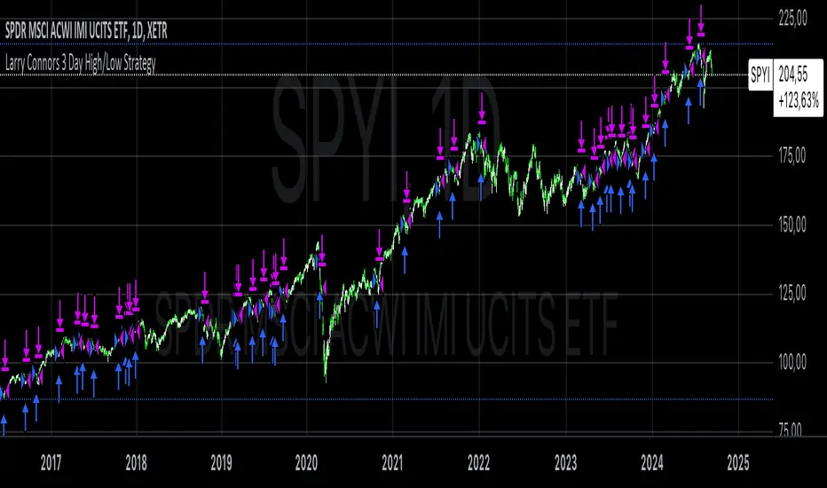
Scaled Historical ATR [SS]Hello again everyone,
This is the Scaled ATR Range indicator. This was done in response to an article/analysis I posted regarding the expected high and range on SPX. I would encourage you to read it here:
Essentially, I took SPX data, scaled it to correct for inflation, then calculated the ATR for Bullish years to get our average range to expect and our close range to expected.
I accomplished this analysis using Excel; however, I figured Pinescript would handle this type of task more elegantly, and I was correct!
This indicator is the result.
What it does:
This indicator permits the analyst to select a historic period in time. The indicator will then scale the period into returns and convert the range to a corrected range based on the current position of the ticker. How it does this is by converting the returns of the historic period selected, then multiplying the returns by the current period open, to ensure that the range amounts are corrected for inflation and natural growth of a ticker.
I say analyst because this indicator is intended to be used by both professional and recreational analysts, to give them an easy way to:
a) Scale historic data and correct it based on the current rate; and
b) Offer insight into a ticker’s ATR and behaviour during bullish and bearish periods.
Prior to this indicator, the only way to do this would be manually or the use of statistical software.
How to use?
The indicator’s use is quite simple. Once launched, the indicator will ask the user to input a timeframe period that the user is interested in assessing. In the main chart above, I chose SPX between 1995 and 2001.
The user can further filter down the data using the settings menu. In the settings menu, there is an option to filter by “All”, “Bullish Periods” or “Bearish Periods”.
Filtering by “All”
Filtering by “All” will include all candles selected within the timeframe. This includes both bearish and bullish candles. It will give you the averaged out range for the entire period of time, including both bearish and bullish instances.
Filtering by “Bullish”
Filtering by “Bullish” will omit any red candles from the analysis. It will only return the ATR ranges for green, bullish candles.
Filtering by “Bearish”
Inverse to filtering by Bullish, if you filter by Bearish, it will only include the red, bearish candles in the analysis.
My suggestion? If you are trying to determine t he likely outcome of a bullish year, filter by Bullish instances. If you want the likely outcome of a bearish year, filter by Bearish.
Other features of the Indicator:
The indicator will display the current period statistics. In the main chart above, you can see that the current ranges for this year are displayed. This allows you to do a side by side comparison of the current period vs. the historic period you are looking at. This can alert you to further upside, further downside and the anticipated close range. It can also alert you to whether or not we are following a similar trajectory as the historical periods you are looking at.
As well, the indicator will list target prices for the current period based on the historical periods you are looking at. This helps to put things into perspective.
Concluding Remarks
And that is the indicator in a nutshell! I encourage you to read the article I linked above to see how you may use it in an analysis. This would be the best example of a real world application of this indicator!
Otherwise, I hope you enjoy and, as always, safe trades!
TASC 2023.05 Cong Adaptive Moving Average█ OVERVIEW
TASC's May 2023 edition of Traders' Tips features an article titled "An Adaptive Moving Average For Swing Trading" by Scott Cong. The article presents a new adaptive moving average (AMA) that adjusts its parameters automatically based on market volatility. The AMA tracks price closely during trending movements and remains flat during congestion areas.
█ CONCEPTS
Conventional moving averages (MAs) use a fixed lookback period, which may lead to limited performance in constantly changing market conditions. Perry Kaufman's adaptive moving average , first described in his 1995 book Smarter Trading, is a great example of how an AMA can self-adjust to adapt to changing environments. Scott Cong draws inspiration from Kaufman's approach and proposes a new way to calculate the AMA smoothing factor.
█ CALCULATIONS
Following Perry Kaufman's approach, Scott Cong's AMA is calculated progressively as:
AMA = α * Close + (1 − α) * AMA(1),
where:
Close = Close of the current bar
AMA(1) = AMA value of the previous bar
α = Smoothing factor between 0 and 1, defined by the lookback period
The smoothing factor determines the performance of AMA. In Cong's approach, it is calculated as:
α = Result / Effort,
where:
Result = Highest price of the n period − Lowest price of the n period
Effort = Sum(TR, n ), where TR stands for Wilder’s true range values of individual bars of the n period
n = Lookback period
As the price range is always no greater than the total journey, α is ensured to be between 0 and 1.
Cong Adaptive Moving AverageDr. Scott Cong's new adaptation of an adaptive moving average (AMA), featured in TASC March 2023.
It adjusts its parameters automatically according to the volatility of market, tracking price closely in trending movement, staying flat in congestion areas.
Perry Kaufman’s adaptive moving average, first described in his 1995 book Smarter Trading, is a great example of how an AMA can self-adjust to adapt to changing environments. This indicator presents a new scheme for an adaptive moving average that is responsive, smooth, and robust.

Intrabar Efficiency Ratio█ OVERVIEW
This indicator displays a directional variant of Perry Kaufman's Efficiency Ratio, designed to gauge the "efficiency" of intrabar price movement by comparing the sum of movements of the lower timeframe bars composing a chart bar with the respective bar's movement on an average basis.
█ CONCEPTS
Efficiency Ratio (ER)
Efficiency Ratio was first introduced by Perry Kaufman in his 1995 book, titled "Smarter Trading". It is the ratio of absolute price change to the sum of absolute changes on each bar over a period. This tells us how strong the period's trend is relative to the underlying noise. Simply put, it's a measure of price movement efficiency. This ratio is the modulator utilized in Kaufman's Adaptive Moving Average (KAMA), which is essentially an Exponential Moving Average (EMA) that adapts its responsiveness to movement efficiency.
ER's output is bounded between 0 and 1. A value of 0 indicates that the starting price equals the ending price for the period, which suggests that price movement was maximally inefficient. A value of 1 indicates that price had travelled no more than the distance between the starting price and the ending price for the period, which suggests that price movement was maximally efficient. A value between 0 and 1 indicates that price had travelled a distance greater than the distance between the starting price and the ending price for the period. In other words, some degree of noise was present which resulted in reduced efficiency over the period.
As an example, let's say that the price of an asset had moved from $15 to $14 by the end of a period, but the sum of absolute changes for each bar of data was $4. ER would be calculated like so:
ER = abs(14 - 15)/4 = 0.25
This suggests that the trend was only 25% efficient over the period, as the total distanced travelled by price was four times what was required to achieve the change over the period.
Intrabars
Intrabars are chart bars at a lower timeframe than the chart's. Each 1H chart bar of a 24x7 market will, for example, usually contain 60 intrabars at the LTF of 1min, provided there was market activity during each minute of the hour. Mining information from intrabars can be useful in that it offers traders visibility on the activity inside a chart bar.
Lower timeframes (LTFs)
A lower timeframe is a timeframe that is smaller than the chart's timeframe. This script determines which LTF to use by examining the chart's timeframe. The LTF determines how many intrabars are examined for each chart bar; the lower the timeframe, the more intrabars are analyzed, but fewer chart bars can display indicator information because there is a limit to the total number of intrabars that can be analyzed.
Intrabar precision
The precision of calculations increases with the number of intrabars analyzed for each chart bar. As there is a 100K limit to the number of intrabars that can be analyzed by a script, a trade-off occurs between the number of intrabars analyzed per chart bar and the chart bars for which calculations are possible.
Intrabar Efficiency Ratio (IER)
Intrabar Efficiency Ratio applies the concept of ER on an intrabar level. Rather than comparing the overall change to the sum of bar changes for the current chart's timeframe over a period, IER compares single bar changes for the current chart's timeframe to the sum of absolute intrabar changes, then applies smoothing to the result. This gives an indication of how efficient changes are on the current chart's timeframe for each bar of data relative to LTF bar changes on an average basis. Unlike the standard ER calculation, we've opted to preserve directional information by not taking the absolute value of overall change, thus allowing it to be utilized as a momentum oscillator. However, by taking the absolute value of this oscillator, it could potentially serve as a replacement for ER in the design of adaptive moving averages.
Since this indicator preserves directional information, IER can be regarded as similar to the Chande Momentum Oscillator (CMO) , which was presented in 1994 by Tushar Chande in "The New Technical Trader". Both CMO and ER essentially measure the same relationship between trend and noise. CMO simply differs in scale, and considers the direction of overall changes.
█ FEATURES
Display
Three different display types are included within the script:
• Line : Displays the middle length MA of the IER as a line .
Color for this display can be customized via the "Line" portion of the "Visuals" section in the script settings.
• Candles : Displays the non-smooth IER and two moving averages of different lengths as candles .
The `open` and `close` of the candle are the longest and shortest length MAs of the IER respectively.
The `high` and `low` of the candle are the max and min of the IER, longest length MA of the IER, and shortest length MA of the IER respectively.
Colors for this display can be customized via the "Candles" portion of the "Visuals" section in the script settings.
• Circles : Displays three MAs of the IER as circles .
The color of each plot depends on the percent rank of the respective MA over the previous 100 bars.
Different colors are triggered when ranks are below 10%, between 10% and 50%, between 50% and 90%, and above 90%.
Colors for this display can be customized via the "Circles" portion of the "Visuals" section in the script settings.
With either display type, an optional information box can be displayed. This box shows the LTF that the script is using, the average number of lower timeframe bars per chart bar, and the number of chart bars that contain LTF data.
Specifying intrabar precision
Ten options are included in the script to control the number of intrabars used per chart bar for calculations. The greater the number of intrabars per chart bar, the fewer chart bars can be analyzed.
The first five options allow users to specify the approximate amount of chart bars to be covered:
• Least Precise (Most chart bars) : Covers all chart bars by dividing the current timeframe by four.
This ensures the highest level of intrabar precision while achieving complete coverage for the dataset.
• Less Precise (Some chart bars) & More Precise (Less chart bars) : These options calculate a stepped LTF in relation to the current chart's timeframe.
• Very precise (2min intrabars) : Uses the second highest quantity of intrabars possible with the 2min LTF.
• Most precise (1min intrabars) : Uses the maximum quantity of intrabars possible with the 1min LTF.
The stepped lower timeframe for "Less Precise" and "More Precise" options is calculated from the current chart's timeframe as follows:
Chart Timeframe Lower Timeframe
Less Precise More Precise
< 1hr 1min 1min
< 1D 15min 1min
< 1W 2hr 30min
> 1W 1D 60min
The last five options allow users to specify an approximate fixed number of intrabars to analyze per chart bar. The available choices are 12, 24, 50, 100, and 250. The script will calculate the LTF which most closely approximates the specified number of intrabars per chart bar. Keep in mind that due to factors such as the length of a ticker's sessions and rounding of the LTF, it is not always possible to produce the exact number specified. However, the script will do its best to get as close to the value as possible.
Specifying MA type
Seven MA types are included in the script for different averaging effects:
• Simple
• Exponential
• Wilder (RMA)
• Weighted
• Volume-Weighted
• Arnaud Legoux with `offset` and `sigma` set to 0.85 and 6 respectively.
• Hull
Weighting
This script includes the option to weight IER values based on the percent rank of absolute price changes on the current chart's timeframe over a specified period, which can be enabled by checking the "Weigh using relative close changes" option in the script settings. This places reduced emphasis on IER values from smaller changes, which may help to reduce noise in the output.
█ FOR Pine Script™ CODERS
• This script imports the recently published lower_ltf library for calculating intrabar statistics and the optimal lower timeframe in relation to the current chart's timeframe.
• This script uses the recently released request.security_lower_tf() Pine Script™ function discussed in this blog post .
It works differently from the usual request.security() in that it can only be used on LTFs, and it returns an array containing one value per intrabar.
This makes it much easier for programmers to access intrabar information.
• This script implements a new recommended best practice for tables which works faster and reduces memory consumption.
Using this new method, tables are declared only once with var , as usual. Then, on the first bar only, we use table.cell() to populate the table.
Finally, table.set_*() functions are used to update attributes of table cells on the last bar of the dataset.
This greatly reduces the resources required to render tables.
Look first. Then leap.

cndevLibrary "cndev"
This function returns the inverse of cumulative normal distribution function
Reference:
The Full Monte, by Boris Moro, Union Bank of Switzerland . RISK 1995(2)
CNDEV(U)
Returns the inverse of cumulative normal distribution function
Parameters:
U : float,
Returns: float.