HSM TOOLS//@version=5
indicator("HSM TOOLS", overlay=true, max_lines_count=500, max_labels_count=5, max_boxes_count=500)
// General Settings Inputs
TZI = input.string (defval="UTC -4", title="Timezone Selection", options= , tooltip="Select the Timezone. ( Shifts Chart Elements )", group="Global Settings")
Timezone = TZI == "UTC -10" ? "GMT-10:00" : TZI == "UTC -7" ? "GMT-07:00" : TZI == "UTC -6" ? "GMT-06:00" : TZI == "UTC -5" ? "GMT-05:00" : TZI == "UTC -4" ? "GMT-04:00" : TZI == "UTC -3" ? "GMT-03:00" : TZI == "UTC +0" ? "GMT+00:00" : TZI == "UTC +1" ? "GMT+01:00" : TZI == "UTC +2" ? "GMT+02:00" : TZI == "UTC +3" ? "GMT+03:00" : TZI == "UTC +3:30" ? "GMT+03:30" : TZI == "UTC +4" ? "GMT+04:00" : TZI == "UTC +5" ? "GMT+05:00" : TZI == "UTC +5:30" ? "GMT+05:30" : TZI == "UTC +6" ? "GMT+06:00" : TZI == "UTC +7" ? "GMT+07:00" : TZI == "UTC +8" ? "GMT+08:00" : TZI == "UTC +9" ? "GMT+09:00" : TZI == "UTC +9:30" ? "GMT+09:30" : TZI == "UTC +10" ? "GMT+10:00" : TZI == "UTC +10:30" ? "GMT+10:30" : TZI == "UTC +11" ? "GMT+11:00" : TZI == "UTC +13" ? "GMT+13:00" : "GMT+13:45"
inputMaxInterval = input.int (31, title="Hide Indicator Above Specified Minutes", tooltip="Above 30Min, Chart Will Become Messy & Unreadable", group="Global Settings")
// Session options
ShowTSO = input.bool (true, title="Show Today's Session Only", group="Session Options", tooltip="Hide Historical Sessions")
ShowTWO = input.bool (true, title="Show Current Week's Sessions Only", group="Session Options", tooltip="Show All Sessions from the current week")
SL4W = input.bool (true, title="Show Last 4 Week Sessions", group="Session Options", tooltip="Show All Sessions from Last Four Weeks \nShould Disable Current Week Session to Work")
ShowSFill = input.bool (false, title="Show Session Highlighting", group="Session Options", tooltip="Highlights Session from Top of the Chart to Bottom")
//----------------------------------------------
// Historical Lines
ShowMOPL = input.bool (title="Midnight Historical Price Lines", defval=false, group="Historical Lines", tooltip="Shows Historical Midnight Price Lines")
MOLHist = input.bool (title="Midnight Historical Vertical Lines", defval=true, group="Historical Lines", tooltip="Shows Historical Midnight Vertical Lines")
ShowPrev = input.bool (false, title="Misc. Historical Price Lines", group="Historical Lines", tooltip="Makes Chart Cluttered, Use For Backtesting Only")
//----------------------------------------------
// Session Bool
ShowLondon = input.bool (false, "", inline="LONDON", group="Sessions", tooltip="01:00 to 05:00")
ShowNY = input.bool (false, "", inline="NY", group="Sessions", tooltip="07:00 to 10:00")
ShowLC = input.bool (false, "", inline="LC", group="Sessions", tooltip="10:00 to 12:00")
ShowPM = input.bool (false, "",inline="PM", group="Sessions", tooltip="13:00 to 16:00")
ShowAsian = input.bool (false, "",inline="ASIA2", group="Sessions", tooltip="20:00 to 00:00")
ShowFreeSesh = input.bool (false, "",inline="FREE", group="Sessions", tooltip="Custom Session")
// Session Strings
txt2 = input.string ("LONDON", title="", inline="LONDON", group="Sessions")
txt3 = input.string ("NEW YORK", title="", inline="NY", group="Sessions")
txt4 = input.string ("LDN CLOSE", title="", inline="LC", group="Sessions")
txt5 = input.string ("AFTERNOON", title="", inline="PM", group="Sessions")
txt6 = input.string ("ASIA", title="", inline="ASIA2", group="Sessions")
txt9 = input.string ("FREE SESH", title="", inline="FREE", group="Sessions")
// CBDR = input.session ('1400-2000:1234567', "", inline="CBDR", group="Sessions")
// ASIA = input.session ('2000-0000:1234567', "", inline="ASIA", group="Sessions")
// Session Times
LDNsesh = input.session ('0200-0500:1234567', "", inline="LONDON", group="Sessions")
NYsesh = input.session ('0700-1000:1234567', "", inline="NY", group="Sessions")
LCsesh = input.session ('1000-1200:1234567', "", inline="LC", group="Sessions")
PMsesh = input.session ('1300-1600:1234567', "", inline="PM", group="Sessions")
ASIA2sesh = input.session ('2000-2359:1234567', "", inline="ASIA2", group="Sessions")
FreeSesh = input.session ('0000-0000:1234567', "", inline="FREE", group="Sessions")
// Session Color
LSFC = input.color (color.new(#787b86, 90), "", inline="LONDON", group="Sessions")
NYSFC = input.color (color.new(#787b86, 90), "",inline="NY", group="Sessions")
LCSFC = input.color (color.new(#787b86, 90), "",inline="LC", group="Sessions")
PMSFC = input.color (color.new(#787b86, 90), "",inline="PM", group="Sessions")
ASFC = input.color (color.new(#787b86, 90), "",inline="ASIA2", group="Sessions")
FSFC = input.color (color.new(#787b86, 90), "",inline="FREE", group="Sessions")
//----------------------------------------------
// Vertical Line Bool
ShowMOP = input.bool (title="", defval=true, inline="MOP", group="Vertical Lines", tooltip="00:00 AM")
txt12 = input.string ("MIDNIGHT", title="", inline="MOP", group="Vertical Lines")
ShowLOP = input.bool (title="", defval=false, inline="LOP", group="Vertical Lines", tooltip="03:00 AM")
txt14 = input.string ("LONDON", title="", inline="LOP", group="Vertical Lines")
ShowNYOP = input.bool (title="", defval=true, inline="NYOP", group="Vertical Lines", tooltip="08:30 AM")
txt15 = input.string ("NEW YORK", title="", inline="NYOP", group="Vertical Lines")
ShowEOP = input.bool (title="", defval=false, inline="EOP", group="Vertical Lines", tooltip="09:30 AM")
txt16 = input.string ("EQUITIES", title="", inline="EOP", group="Vertical Lines")
// Vertical Line Color
MOPColor = input.color (color.new(#787b86, 0), "", inline="MOP", group="Vertical Lines")
LOPColor = input.color (color.rgb(0,128,128,60), "", inline="LOP", group="Vertical Lines")
NYOPColor = input.color (color.rgb(0,128,128,60), "", inline="NYOP", group="Vertical Lines")
EOPColor = input.color (color.rgb(0,128,128,60), "", inline="EOP", group="Vertical Lines")
// Vertical LineStyle
Midnight_Open_LS = input.string ("Dotted", "", options= , inline="MOP", group="Vertical Lines")
london_Open_LS = input.string ("Solid", "", options= , inline="LOP", group="Vertical Lines")
NY_Open_LS = input.string ("Solid", "", options= , inline="NYOP", group="Vertical Lines")
Equities_Open_LS = input.string ("Solid", "", options= , inline="EOP", group="Vertical Lines")
// Vertical LineWidth
Midnight_Open_LW = input.string ("1px", "", options= , inline="MOP", group="Vertical Lines")
London_Open_LW = input.string ("1px", "", options= , inline="LOP", group="Vertical Lines")
NY_Open_LW = input.string ("1px", "", options= , inline="NYOP", group="Vertical Lines")
Equities_Open_LW = input.string ("1px", "", options= , inline="EOP", group="Vertical Lines")
//----------------------------------------------
// Opening Price Bool
ShowMOPP = input.bool (title="", defval=true, inline="MOPP", group="Opening Price Lines", tooltip="00:00 AM")
txt13 = input.string ("MIDNIGHT", title="", inline="MOPP", group="Opening Price Lines")
ShowNYOPP = input.bool (title="", defval=false, inline="NYOPP", group="Opening Price Lines", tooltip="08:30 AM")
txt17 = input.string ("NEW YORK", title="", inline="NYOPP", group="Opening Price Lines")
ShowEOPP = input.bool (title="", defval=false, inline="EOPP", group="Opening Price Lines", tooltip="09:30 AM")
txt18 = input.string ("EQUITIES", title="", inline="EOPP", group="Opening Price Lines")
ShowAFTPP = input.bool (title="", defval=false, inline="AFTOPP", group="Opening Price Lines", tooltip="01:30 PM")
txt1330 = input.string ("AFTERNOON", title="", inline="AFTOPP", group="Opening Price Lines")
// Opening Price Color
MOPColP = input.color (color.new(#787b86, 0), "", inline="MOPP", group="Opening Price Lines")
NYOPColP = input.color (color.new(#787b86, 0), "", inline="NYOPP", group="Opening Price Lines")
EOPColP = input.color (color.new(#787b86, 0), "", inline="EOPP", group="Opening Price Lines")
AFTOPColP = input.color (color.new(#787b86, 0), "", inline="AFTOPP", group="Opening Price Lines")
// Opening Price LineStyle
MOPLS = input.string ("Dotted", "", options= , inline="MOPP", group="Opening Price Lines")
NYOPLS = input.string ("Dotted", "", options= , inline="NYOPP", group="Opening Price Lines")
EOPLS = input.string ("Dotted", "", options= , inline="EOPP", group="Opening Price Lines")
AFTOPLS = input.string ("Dotted", "", options= , inline="AFTOPP", group="Opening Price Lines")
// Opening Price LineWidth
i_MOPLW = input.string ("1px", "", options= , inline="MOPP", group="Opening Price Lines")
i_NYOPLW = input.string ("1px", "", options= , inline="NYOPP", group="Opening Price Lines")
i_EOPLW = input.string ("1px", "", options= , inline="EOPP", group="Opening Price Lines")
i_AFTOPLW = input.string ("1px", "", options= , inline="AFTOPP", group="Opening Price Lines")
//----------------------------------------------
// W&M Bool
ShowWeekOpen = input.bool (defval=false, title="", tooltip="Draw Weekly Open Price Line", group="HTF Opening Price Lines", inline="WO")
showMonthOpen = input.bool (defval=false, title="", tooltip="Draw Monthly Open Price Line", group="HTF Opening Price Lines", inline="MO")
// W&M String
txt19 = input.string ("WEEKLY", title="", inline="WO", group="HTF Opening Price Lines")
txt20 = input.string ("MONTHLY", title="", inline="MO", group="HTF Opening Price Lines")
// W&M Color
i_WeekOpenCol = input.color (title="", defval=color.new(#787b86, 0), group="HTF Opening Price Lines", inline="WO")
i_MonthOpenCol = input.color (title="", tooltip="", defval=color.new(#787b86, 0), group="HTF Opening Price Lines", inline="MO")
// W&M LineStyle
WOLS = input.string ("Dotted", "", options= , inline="WO", group="HTF Opening Price Lines")
MOLS = input.string ("Dotted", "", options= , inline="MO", group="HTF Opening Price Lines")
// W&M LineWidth
i_WOPLW = input.string ("1px", "", options= , inline="WO", group="HTF Opening Price Lines")
i_MONPLW = input.string ("1px", "", options= , inline="MO", group="HTF Opening Price Lines")
//----------------------------------------------
// CBDR, ASIA & FLOUT
ShowCBDR = input.bool (true, "", inline='CBDR', group="CBDR, ASIA & FLOUT")
ShowASIA = input.bool (true, "", inline='ASIA', group="CBDR, ASIA & FLOUT")
ShowFLOUT = input.bool (false, "", inline='FLOUT', group="CBDR, ASIA & FLOUT")
// Strings
txt0 = input.string ("CBDR", title="", inline="CBDR", group="CBDR, ASIA & FLOUT", tooltip="16:00 to 20:00 \nSD Increments of 1")
txt1 = input.string ("ASIA", title="", inline="ASIA", group="CBDR, ASIA & FLOUT", tooltip="20:00 to 00:00 \nSD Increments of 1")
txt7 = input.string ("FLOUT", title="", inline="FLOUT", group="CBDR, ASIA & FLOUT", tooltip="16:00 to 00:00 \nSD Increments of 0.5")
// Color
CBDRBoxCol = input.color (color.new(#787b86, 0),"", inline='CBDR', group="CBDR, ASIA & FLOUT")
ASIABoxCol = input.color (color.new(#787b86, 0), "", inline='ASIA', group="CBDR, ASIA & FLOUT")
FLOUTBoxCol = input.color (color.new(#787b86, 0),"", inline='FLOUT', group="CBDR, ASIA & FLOUT")
// Extras
box_text_cbdr = input.bool (true, "Show Text", inline="CBDR", group="CBDR, ASIA & FLOUT")
box_text_cbdr_col = input.color (color.new(color.gray, 80), "", inline="CBDR", group="CBDR, ASIA & FLOUT")
bool_cbdr_dev = input.bool (true, "SD", inline="CBDR", group="CBDR, ASIA & FLOUT")
box_text_asia = input.bool (true, "Show Text", inline="ASIA", group="CBDR, ASIA & FLOUT")
box_text_asia_col = input.color (color.new(color.gray, 80), "", inline="ASIA", group="CBDR, ASIA & FLOUT")
bool_asia_dev = input.bool (true, "SD", inline="ASIA", group="CBDR, ASIA & FLOUT")
box_text_flout = input.bool (true, "Show Text", inline="FLOUT", group="CBDR, ASIA & FLOUT")
box_text_flout_col = input.color (color.new(color.gray, 80), "", inline="FLOUT", group="CBDR, ASIA & FLOUT")
bool_flout_dev = input.bool (true, "SD", inline="FLOUT", group="CBDR, ASIA & FLOUT")
// Table
// SD Lines
ShowDevLN = input.bool (title="", defval=true, inline="DEVLN", group="Standard Deviation", tooltip="Deviation Lines")
DEVLNTXT = input.string ("SD LINES", title="", inline="DEVLN", group="Standard Deviation")
DevLNCol = input.color (color.new(#787b86, 0), "", inline="DEVLN", group="Standard Deviation")
DEVLS = input.string ("Solid", "", options= , inline="DEVLN", group="Standard Deviation")
i_DEVLW = input.string ("1px", "", options= , inline="DEVLN", group="Standard Deviation")
DEVLSS = DEVLS=="Solid" ? line.style_solid : DEVLS == "Dotted" ? line.style_dotted : line.style_dashed
DEVLW = i_DEVLW=="1px" ? 1 : i_DEVLW == "2px" ? 2 : i_DEVLW == "3px" ? 3 : i_DEVLW == "4px" ? 4 : 5
ShowDev = input.bool (false, '', inline="DEV", group="Standard Deviation")
txt8 = input.string ("SD COUNT", title="", inline="DEV", group="Standard Deviation")
SDCountCol = input.color (color.new(#787b86, 0), "", inline="DEV", group="Standard Deviation")
DevInput = input.string ("2 SD", "", options= , inline="DEV", group="Standard Deviation")
DevDirection = input.string ("Both", "", options= , inline="DEV", group="Standard Deviation", tooltip="SD Count, NULL, SD Count, SD Direction")
DevCount = DevInput == "1 SD" ? 1 : DevInput == "2 SD" ? 2 : DevInput == "3 SD" ? 3 : 4
Auto_Select = input.bool (false, "", group="Standard Deviation", inline="AUTOSD", tooltip="Auto SD Selection | Charter Content, Range Table \nMight Bug Out On Mondays" )
txtSD = input.string ("AUTO SD", "", group="Standard Deviation", inline="AUTOSD")
Tab1txtCol = input.color (color.new(#808080, 0), "", inline='AUTOSD', group="Standard Deviation")
TabOptionShow = input.string ("Show Table", "", options= , inline="AUTOSD", group="Standard Deviation")
Stats = TabOptionShow == "Show Table" ? true : false
TabOption1 = input.string ("Top Right", "", options= , inline="AUTOSD", group="Standard Deviation")
tabinp1 = TabOption1 == "Top Left" ? position.top_left : TabOption1 == "Top Center" ? position.top_center : TabOption1 == "Top Right" ? position.top_right : TabOption1 == "Middle Left" ? position.middle_left : TabOption1 == "Middle Right" ? position.middle_right : TabOption1 == "Bottom Left" ? position.bottom_left : TabOption1 == "Bottom Center" ? position.bottom_center : position.bottom_right
L_Prof = true
CellBG = color.new(#131722, 100)
//----------------------------------------------
// Day Of Week & Labels
// Label Settings Inputs
ShowLabel = input.bool (true, title="", inline="Glabel", group="Day Of Week & Labels")
txt21 = input.string ("LABEL", title="", inline="Glabel", group="Day Of Week & Labels")
LabelColor = input.color (color.rgb(0,0,0,100), "", inline="Glabel", group="Day Of Week & Labels")
LabelSizeInput = input.string ("Normal", "", options= , inline="Glabel", group="Day Of Week & Labels")
Terminusinp = input.string ("Terminus @ Current Time +1hr", "", options = , inline="Glabel", group="Day Of Week & Labels", tooltip="Select Label Size & Color & Terminus \nHistorical Price Lines needs to be toggled off for using Terminus")
ShowLabelText = input.bool (true, title="", inline="label", group="Day Of Week & Labels")
txt22 = input.string ("LABEL TEXT", title="", inline="label", group="Day Of Week & Labels")
LabelTextColor = input.color (color.new(#787b86, 0), title="", inline="label", group="Day Of Week & Labels")
LabelTextOptioninput = input.string ("Time", "", options= , inline="label", group="Day Of Week & Labels", tooltip="Choose Between Descriptive Text as Label or Time \nShow/Hide Prices on Labels")
ShowPricesBool = input.string ("Hide Prices", title="", options= , group="Day Of Week & Labels", inline="label")
ShowPrices = ShowPricesBool == "Show Prices" ? true : false
showDOW = input.bool (true, title="", inline="DOW", group="Day Of Week & Labels")
txt24 = input.string ("DAY OF WEEK", title="", inline="DOW", group="Day Of Week & Labels")
i_DOWCol = input.color (color.new(#787b86, 0), title="", inline="DOW", group="Day Of Week & Labels")
DOWTime = input.int (defval = 12, title="", inline="DOW", group="Day Of Week & Labels")
DOWLoc_inpt = input.string ("Bottom", "", options = , inline="DOW", group="Day Of Week & Labels", tooltip="DOW Color, Time Alignment, Vertical Location")
DOWLoc = DOWLoc_inpt == "Bottom" ? location.bottom : location.top
//----------------------------------------------
BIAS_M_Bool = input.bool (false, "", group="BIAS & NOTES PRECONFIG", inline="stats")
txt100 = input.string ("BIAS", title="", inline="stats", group="BIAS & NOTES PRECONFIG")
TableBG2 = color.new(#131722, 100)
Tab2txtCol = input.color (color.new(#787b86, 0), "", inline='stats', group="BIAS & NOTES PRECONFIG")
TabOption2 = input.string ("Bottom Right", "", options= , inline="stats", group="BIAS & NOTES PRECONFIG")
tabinp2 = TabOption2 == "Top Left" ? position.top_left : TabOption2 == "Top Center" ? position.top_center : TabOption2 == "Top Right" ? position.top_right : TabOption2 == "Middle Left" ? position.middle_left : TabOption2 == "Middle Right" ? position.middle_right : TabOption2 == "Bottom Left" ? position.bottom_left : TabOption2 == "Bottom Center" ? position.bottom_center : position.bottom_right
notesbool = false
NOTES_M_Bool = input.bool (true, "", group="BIAS & NOTES PRECONFIG", inline="stats2")
txt101 = input.string ("NOTES", title="", inline="stats2", group="BIAS & NOTES PRECONFIG")
Tab3txtCol = input.color (color.new(#787b86, 0), "", inline='stats2', group="BIAS & NOTES PRECONFIG")
TabOption3 = input.string ("Top Center", "", options= , inline="stats2", group="BIAS & NOTES PRECONFIG")
tabinp3 = TabOption3 == "Top Left" ? position.top_left : TabOption3 == "Top Center" ? position.top_center : TabOption3 == "Top Right" ? position.top_right : TabOption3 == "Middle Left" ? position.middle_left : TabOption3 == "Middle Right" ? position.middle_right : TabOption3 == "Bottom Left" ? position.bottom_left : TabOption3 == "Bottom Center" ? position.bottom_center : position.bottom_right
BIASbool1 = input.bool (true, '', inline="BIAS1", group="BIAS & NOTES")
txt52 = input.string ("DXY ", title="", inline="BIAS1", group="BIAS & NOTES")
BIASOption1 = input.string ("Unclear", options= , title="", inline="BIAS1", group="BIAS & NOTES")
BIASbool2 = input.bool (true, '', inline="BIAS2", group="BIAS & NOTES")
txt53 = input.string ("SPX ", title="", inline="BIAS2", group="BIAS & NOTES")
BIASOption2 = input.string ("Unclear", options= , title="", inline="BIAS2", group="BIAS & NOTES")
BIASbool3 = input.bool (true, '', inline="BIAS3", group="BIAS & NOTES")
txt54 = input.string ("DOW ", title="", inline="BIAS3", group="BIAS & NOTES")
BIASOption3 = input.string ("Unclear", options= , title="", inline="BIAS3", group="BIAS & NOTES")
BIASbool4 = input.bool (true, '', inline="BIAS4", group="BIAS & NOTES")
txt55 = input.string ("NAS ", title="", inline="BIAS4", group="BIAS & NOTES")
BIASOption4 = input.string ("Unclear", options= , title="", inline="BIAS4", group="BIAS & NOTES")
notes = input.text_area ("@hiran.invest", "Notes", group = "BIAS & NOTES")
//--------------------END OF INPUTS--------------------//
// Pre-Def
DOM = (timeframe.multiplier <= inputMaxInterval) and (timeframe.isintraday)
newDay = ta.change(dayofweek)
newWeek = ta.change(weekofyear)
newMonth = ta.change(time("M"))
transparentcol = color.rgb(255,255,255,100)
LSVLC = color.rgb(255,255,255,100)
NYSVLC = color.rgb(255,255,255,100)
PMSVLC = color.rgb(255,255,255,100)
ASVLC = color.rgb(255,255,255,100)
LSVLS = "dotted"
NYSVLS = "dotted"
PMSVLS = "dotted"
ASVLS = "dotted"
// Functions
isToday = false
if year(timenow) == year(time) and month(timenow) == month(time) and dayofmonth(timenow) == dayofmonth(time)
isToday := true
// Current Week
thisweek = year(timenow) == year(time) and weekofyear(timenow) == weekofyear(time)
LastOneWeek = year(timenow) == year(time) and weekofyear(timenow-604800000) == weekofyear(time)
LastTwoWeek = year(timenow) == year(time) and weekofyear(timenow-1209600000) == weekofyear(time)
LastThreeWeek = year(timenow) == year(time) and weekofyear(timenow-1814400000) == weekofyear(time)
LastFourWeek = year(timenow) == year(time) and weekofyear(timenow-2419200000) == weekofyear(time)
Last4Weeks = false
if thisweek == true or LastOneWeek == true or LastTwoWeek == true or LastThreeWeek == true or LastFourWeek == true
Last4Weeks := true
// Function to draw Vertical Lines
vline(Start, Color, linestyle, LineWidth) =>
line.new(x1=Start, y1=low - ta.tr, x2=Start, y2=high + ta.tr, xloc=xloc.bar_time, extend=extend.both, color=Color, style=linestyle, width=LineWidth)
// Function to convert forex pips into whole numbers
atr = ta.atr(14)
toWhole(number) =>
if syminfo.type == "forex" // This method only works on forex pairs
_return = atr < 1.0 ? (number / syminfo.mintick) / 10 : number
_return := atr >= 1.0 and atr < 100.0 and syminfo.currency == "JPY" ? _return * 100 : _return
else
number
// Function for determining the Start of a Session (taken from the Pinescript manual: www.tradingview.com )
SessionBegins(sess) =>
t = time("", sess , Timezone)
DOM and (not barstate.isfirst) and na(t ) and not na(t)
// BarIn Session
BarInSession(sess) =>
time(timeframe.period, sess, Timezone) != 0
// Label Type Logic
var SFistrue = true
if LabelTextOptioninput == "Time"
SFistrue := true
else
SFistrue := false
// Session String to int
SeshStartHour(Session) =>
math.round(str.tonumber(str.substring(Session,0,2)))
SeshStartMins(Session) =>
math.round(str.tonumber(str.substring(Session,2,4)))
SeshEndHour(Session) =>
math.round(str.tonumber(str.substring(Session,5,7)))
SeshEndMins(Session) =>
math.round(str.tonumber(str.substring(Session,7,9)))
// Time periods
CBDR = "1600-2000:1234567"
ASIA = "2000-0000:1234567"
FLOUT = "1600-0000:1234567"
midsesh = "0000-1600:1234567"
cbdrOpenTime = timestamp (Timezone, year, month, dayofmonth, SeshStartHour(CBDR), SeshStartMins(CBDR), 00)
cbdrEndTime = timestamp (Timezone, year, month, dayofmonth, SeshEndHour(CBDR), SeshEndMins(CBDR), 00)
asiaOpenTime = timestamp (Timezone, year, month, dayofmonth, SeshStartHour(ASIA), SeshStartMins(ASIA), 00)
asiaEndTime = timestamp (Timezone, year, month, dayofmonth, SeshEndHour(ASIA), SeshEndMins(ASIA), 00)+86400000
floutOpenTime = timestamp (Timezone, year, month, dayofmonth, SeshStartHour(FLOUT), SeshStartMins(FLOUT), 00)
floutEndTime = timestamp (Timezone, year, month, dayofmonth, SeshEndHour(FLOUT), SeshEndMins(FLOUT), 00)+86400000
CBDRTime = time (timeframe.period, CBDR, Timezone)
ASIATime = time (timeframe.period, ASIA, Timezone)
FLOUTTime = time (timeframe.period, FLOUT, Timezone)
LabelOnlyToday = true
// Time Periods
LondonStartTime = timestamp(Timezone, year, month, dayofmonth, SeshStartHour(LDNsesh), SeshStartMins(LDNsesh), 00)
LondonEndTime = timestamp(Timezone, year, month, dayofmonth, SeshEndHour(LDNsesh), SeshEndMins(LDNsesh), 00)
NYStartTime = timestamp(Timezone, year, month, dayofmonth, SeshStartHour(NYsesh), SeshStartMins(NYsesh), 00)
NYEndTime = timestamp(Timezone, year, month, dayofmonth, SeshEndHour(NYsesh), SeshEndMins(NYsesh), 00)
LCStartTime = timestamp(Timezone, year, month, dayofmonth, SeshStartHour(LCsesh), SeshStartMins(LCsesh), 00)
LCEndTime = timestamp(Timezone, year, month, dayofmonth, SeshEndHour(LCsesh), SeshEndMins(LCsesh), 00)
PMStartTime = timestamp(Timezone, year, month, dayofmonth, SeshStartHour(PMsesh), SeshStartMins(PMsesh), 00)
PMEndTime = timestamp(Timezone, year, month, dayofmonth, SeshEndHour(PMsesh), SeshEndMins(PMsesh), 00)
AsianStartTime = timestamp(Timezone, year, month, dayofmonth, SeshStartHour(ASIA2sesh), SeshStartMins(ASIA2sesh), 00)
AsianEndTime = timestamp(Timezone, year, month, dayofmonth, SeshEndHour(ASIA2sesh), SeshEndMins(ASIA2sesh), 00)
FreeStartTime = timestamp(Timezone, year, month, dayofmonth, SeshStartHour(FreeSesh), SeshStartMins(FreeSesh), 00)
FreeEndTime = timestamp(Timezone, year, month, dayofmonth, SeshEndHour(FreeSesh), SeshEndMins(FreeSesh), 00)
MidnightOpenTime = timestamp(Timezone, year, month, dayofmonth, 0, 0, 00)
CLEANUPTIME = timestamp(Timezone, year, month, dayofmonth, 0, 0, 00) - 16200000
LondonOpenTime = timestamp(Timezone, year, month, dayofmonth, 3, 0, 00)
NYOpenTime = timestamp(Timezone, year, month, dayofmonth, 8, 30, 00)
EquitiesOpenTime = timestamp(Timezone, year, month, dayofmonth, 9, 30, 00)
AfternoonOpenTime = timestamp(Timezone, year, month, dayofmonth, 13, 30, 00)
tMidnight = time("1", "0000-0001:1234567", Timezone)
// Cleanup - Remove old drawing objects
Cleanup(days) =>
// Delete old drawing objects
// One day is 86400000 milliseconds
removal_timestamp = (CLEANUPTIME) - (days * 86400000) // Remove every drawing object older than the start of the Today's Midnight
a_allLines = line.all
a_allLabels = label.all
a_allboxes = box.all
// Remove old lines
if array.size(a_allLines) > 0
for i = 0 to array.size(a_allLines) - 1
line_x2 = line.get_x2(array.get(a_allLines, i))
if line_x2 < (removal_timestamp)
line.delete(array.get(a_allLines, i))
// Remove old labels
if array.size(a_allLabels) > 0
for i = 0 to array.size(a_allLabels) - 1
label_x = label.get_x(array.get(a_allLabels, i))
if label_x < removal_timestamp
label.delete(array.get(a_allLabels, i))
// Remove old boxes
if array.size(a_allboxes) > 0
for i = 0 to array.size(a_allboxes) - 1
box_x = box.get_right(array.get(a_allboxes, i))
if box_x < (removal_timestamp - 86400000)
box.delete(array.get(a_allboxes, i))
// End of Cleanup function
// Terminus Function
Terminus(Terminus_Inp)=>
if Terminus_Inp == "Terminus @ Current Time"
_return = timenow
else if Terminus_Inp == "Terminus @ Current Time +15min"
_return = timenow + 900000
else if Terminus_Inp == "Terminus @ Current Time +30min"
_return = timenow + 1800000
else if Terminus_Inp == "Terminus @ Current Time +45min"
_return = timenow + 2700000
else if Terminus_Inp == "Terminus @ Current Time +1hr"
_return = timenow + 3600000
else if Terminus_Inp == "Terminus @ Current Time +2hr"
_return = timenow + 7200000
else
_return = timenow + 10800000
// Linestyle Function
MNOPLS = Midnight_Open_LS=="Solid" ? line.style_solid : Midnight_Open_LS == "Dotted" ? line.style_dotted : line.style_dashed
LNOPLS = london_Open_LS=="Solid" ? line.style_solid : london_Open_LS == "Dotted" ? line.style_dotted : line.style_dashed
NWYOPLS = NY_Open_LS=="Solid" ? line.style_solid : NY_Open_LS == "Dotted" ? line.style_dotted : line.style_dashed
EQOPLS = Equities_Open_LS=="Solid" ? line.style_solid : Equities_Open_LS == "Dotted" ? line.style_dotted : line.style_dashed
MOPLSS = MOPLS=="Solid" ? line.style_solid : MOPLS == "Dotted" ? line.style_dotted : line.style_dashed
NYOPLSS = NYOPLS=="Solid" ? line.style_solid : NYOPLS == "Dotted" ? line.style_dotted : line.style_dashed
EOPLSS = EOPLS=="Solid" ? line.style_solid : EOPLS == "Dotted" ? line.style_dotted : line.style_dashed
AFTOPLSS = AFTOPLS=="Solid" ? line.style_solid : AFTOPLS == "Dotted" ? line.style_dotted : line.style_dashed
WeekOpenLS = WOLS=="Solid" ? line.style_solid : WOLS == "Dotted" ? line.style_dotted : line.style_dashed
MonthOpenLS = MOLS=="Solid" ? line.style_solid : MOLS == "Dotted" ? line.style_dotted : line.style_dashed
// Linewidth Function
MOPLW = Midnight_Open_LW=="1px" ? 1 : Midnight_Open_LW == "2px" ? 2 : Midnight_Open_LW == "3px" ? 3 : Midnight_Open_LW == "4px" ? 4 : 5
LOPLW = London_Open_LW=="1px" ? 1 : London_Open_LW == "2px" ? 2 : London_Open_LW == "3px" ? 3 : London_Open_LW == "4px" ? 4 : 5
NYOPLW = NY_Open_LW=="1px" ? 1 : NY_Open_LW == "2px" ? 2 : NY_Open_LW == "3px" ? 3 : NY_Open_LW == "4px" ? 4 : 5
EOPLW = Equities_Open_LW=="1px" ? 1 : Equities_Open_LW == "2px" ? 2 : Equities_Open_LW == "3px" ? 3 : Equities_Open_LW == "4px" ? 4 : 5
MOPPLW = i_MOPLW=="1px" ? 1 : i_MOPLW == "2px" ? 2 : i_MOPLW == "3px" ? 3 : i_MOPLW == "4px" ? 4 : 5
NYOPPLW = i_NYOPLW=="1px" ? 1 : i_NYOPLW == "2px" ? 2 : i_NYOPLW == "3px" ? 3 : i_NYOPLW == "4px" ? 4 : 5
EOPPLW = i_EOPLW=="1px" ? 1 : i_EOPLW == "2px" ? 2 : i_EOPLW == "3px" ? 3 : i_EOPLW == "4px" ? 4 : 5
AFTOPLW = i_AFTOPLW=="1px" ? 1 : i_AFTOPLW == "2px" ? 2 : i_AFTOPLW == "3px" ? 3 : i_AFTOPLW == "4px" ? 4 : 5
WEEKOPPLW = i_WOPLW=="1px" ? 1 : i_WOPLW == "2px" ? 2 : i_WOPLW == "3px" ? 3 : i_WOPLW == "4px" ? 4 : 5
MONTHOPPLW = i_MONPLW=="1px" ? 1 : i_MONPLW == "2px" ? 2 : i_MONPLW == "3px" ? 3 : i_MONPLW == "4px" ? 4 : 5
// Label Size Function
LabelSize =LabelSizeInput=="Auto" ? size.auto : LabelSizeInput=="Tiny" ? size.tiny : LabelSizeInput=="Small" ? size.small : LabelSizeInput=="Normal" ? size.normal : LabelSizeInput=="Large" ? size.large : size.huge
// Creating Variables
var London_Start_Vline = line.new(x1=na, y1=na, x2=na, xloc=xloc.bar_time, y2=close, color=LSVLC, width=1)
var London_End_Vline = line.new(x1=na, y1=na, x2=na, xloc=xloc.bar_time, y2=close, color=LSVLC, width=1)
var LondonFill = linefill.new(London_Start_Vline, London_End_Vline, LSFC)
var NY_Start_Vline = line.new(x1=na, y1=na, x2=na, xloc=xloc.bar_time, y2=close, color=NYSVLC, width=1)
var NY_End_Vline = line.new(x1=na, y1=na, x2=na, xloc=xloc.bar_time, y2=close, color=NYSVLC, width=1)
var NYFill = linefill.new(NY_Start_Vline, NY_End_Vline, NYSFC)
var LC_Start_Vline = line.new(x1=na, y1=na, x2=na, xloc=xloc.bar_time, y2=close, color=NYSVLC, width=1)
var LC_End_Vline = line.new(x1=na, y1=na, x2=na, xloc=xloc.bar_time, y2=close, color=NYSVLC, width=1)
var LCFill = linefill.new(LC_Start_Vline, LC_End_Vline, LCSFC)
var PM_Start_Vline = line.new(x1=na, y1=na, x2=na, xloc=xloc.bar_time, y2=close, color=PMSVLC, width=1)
var PM_End_Vline = line.new(x1=na, y1=na, x2=na, xloc=xloc.bar_time, y2=close, color=PMSVLC, width=1)
var PMFill = linefill.new(PM_Start_Vline, PM_End_Vline, PMSFC)
var Asian_Start_Vline = line.new(x1=na, y1=na, x2=na, xloc=xloc.bar_time, y2=close, color=ASVLC, width=1)
var Asian_End_Vline = line.new(x1=na, y1=na, x2=na, xloc=xloc.bar_time, y2=close, color=ASVLC, width=1)
var AsianFill = linefill.new(Asian_Start_Vline, Asian_End_Vline, ASFC)
var Free_Start_Vline = line.new(x1=na, y1=na, x2=na, xloc=xloc.bar_time, y2=close, color=ASVLC, width=1)
var Free_End_Vline = line.new(x1=na, y1=na, x2=na, xloc=xloc.bar_time, y2=close, color=ASVLC, width=1)
var FreeFill = linefill.new(Free_Start_Vline, Free_End_Vline, FSFC)
var Midnight_Open = line.new(x1=na, y1=na, x2=na, xloc=xloc.bar_time, y2=close, color=MOPColor, width=1)
var London_Open = line.new(x1=na, y1=na, x2=na, xloc=xloc.bar_time, y2=close, color=LOPColor, width=1)
var NY_Open = line.new(x1=na, y1=na, x2=na, xloc=xloc.bar_time, y2=close, color=NYOPColor, width=1)
var Equities_Open = line.new(x1=na, y1=na, x2=na, xloc=xloc.bar_time, y2=close, color=EOPColor, width=1)
// When a New Day Starts, Start Drawing all lines
if newDay and dayofweek != dayofweek.sunday
// London Session
if (ShowLondon and DOM)
if ShowTSO
line.delete(London_Start_Vline )
line.delete(London_End_Vline )
linefill.delete(LondonFill )
London_Start_Vline := vline(LondonStartTime,transparentcol, line.style_solid, 1)
London_End_Vline := vline(LondonEndTime, transparentcol, line.style_solid, 1)
if ShowSFill
LondonFill := linefill.new(London_Start_Vline, London_End_Vline, LSFC)
// New York Session
if (ShowNY and DOM)
if ShowTSO
line.delete(NY_Start_Vline )
line.delete(NY_End_Vline )
linefill.delete(NYFill )
NY_Start_Vline := vline(NYStartTime, transparentcol, line.style_solid, 1)
NY_End_Vline := vline(NYEndTime, transparentcol, line.style_solid, 1)
if ShowSFill
NYFill := linefill.new(NY_Start_Vline, NY_End_Vline, NYSFC)
// London Close
if (ShowLC and DOM)
if ShowTSO
line.delete(LC_End_Vline )
linefill.delete(LCFill )
LC_Start_Vline := vline(LCStartTime, transparentcol, line.style_solid, 1)
LC_End_Vline := vline(LCEndTime, transparentcol, line.style_solid, 1)
if ShowSFill
LCFill := linefill.new(LC_Start_Vline, LC_End_Vline, LCSFC)
// PM Session
if (ShowPM and DOM)
if ShowTSO
line.delete(PM_Start_Vline )
line.delete(PM_End_Vline )
linefill.delete(PMFill )
PM_Start_Vline := vline(PMStartTime, transparentcol, line.style_solid, 1)
PM_End_Vline := vline(PMEndTime, transparentcol, line.style_solid, 1)
if ShowSFill
PMFill := linefill.new(PM_Start_Vline, PM_End_Vline, PMSFC)
// Asian Session
if (ShowAsian and DOM)
if ShowTSO
line.delete(Asian_Start_Vline )
line.delete(Asian_End_Vline )
linefill.delete(AsianFill )
Asian_Start_Vline := vline(AsianStartTime, transparentcol, line.style_solid, 1)
Asian_End_Vline := vline(AsianEndTime, transparentcol, line.style_solid, 1)
// if dayofweek == dayofweek.friday
// // line.delete(Asian_Start_Vline)
// // line.delete(Asian_End_Vline)
// Asian_Start_Vline := vline(MidnightOpenTime+244800000, transparentcol, line.style_solid, 1)
// Asian_End_Vline := vline(MidnightOpenTime+259200000, transparentcol, line.style_solid, 1)
if ShowSFill
AsianFill := linefill.new(Asian_Start_Vline, Asian_End_Vline, ASFC)
// Free Session
if (ShowFreeSesh and DOM)
if ShowTSO
line.delete(Free_Start_Vline )
line.delete(Free_End_Vline )
linefill.delete(FreeFill )
Free_Start_Vline := vline(FreeStartTime, transparentcol, line.style_solid, 1)
Free_End_Vline := vline(FreeEndTime, transparentcol, line.style_solid, 1)
if ShowSFill
FreeFill := linefill.new(Free_Start_Vline, Free_End_Vline, FSFC)
// Midnight Opening Price
if (ShowMOP and DOM)
if MOLHist == false
line.delete(Midnight_Open )
Midnight_Open := vline(MidnightOpenTime, MOPColor, MNOPLS, MOPLW)
// London Opening Price
if (ShowLOP and DOM)
if ShowTSO
line.delete(London_Open )
London_Open := vline(LondonOpenTime, LOPColor, LNOPLS, LOPLW)
// New York Opening Price
if (ShowNYOP and DOM)
if ShowTSO
line.delete(NY_Open )
NY_Open := vline(NYOpenTime, NYOPColor, NWYOPLS, NYOPLW)
// Equities Opening Price
if (ShowEOP and DOM)
if ShowTSO
line.delete(Equities_Open )
Equities_Open := vline(EquitiesOpenTime, EOPColor, EQOPLS, EOPLW)
// Variables
var label MOPLB = na
var line MOPLN = na
var label NYOPLB = na
var line NYOPLN = na
var label EOPLB = na
var line EOPLN = na
var line AFTLN = na
var label AFTLB = na
// New York Midnight Open Price line
var openMidnight = 0.0
if tMidnight
if not tMidnight
openMidnight := open
else
openMidnight := math.max(open, openMidnight)
if (ShowMOPP and (openMidnight != openMidnight ) and DOM and barstate.isconfirmed)
label.delete(MOPLB )
if ShowMOPL == false
line.delete(MOPLN )
MOPLN := line.new(x1=tMidnight, y1=openMidnight, x2=tMidnight+86400000, xloc=xloc.bar_time, y2=openMidnight, color=MOPColP, style=MOPLSS, width=MOPPLW)
if dayofweek == dayofweek.friday and syminfo.type != "crypto"
line.set_x2(MOPLN, tMidnight+259200000)
if ShowLabel
MOPLB := label.new(x=tMidnight+86400000, y=openMidnight, xloc=xloc.bar_time, color=LabelColor, textcolor=MOPColP, style=label.style_label_left, size=LabelSize, tooltip="Midnight Opening Price")
if dayofweek == dayofweek.friday and syminfo.type != "crypto"
label.set_x(MOPLB, tMidnight+259200000)
if ShowLabelText
if SFistrue
if ShowPrices == true
label.set_text(MOPLB, " 00:00 | " + str.tostring(open))
else
label.set_text(MOPLB, " 00:00 ")
label.set_tooltip(MOPLB, "Midnight Opening Price")
else
if ShowPrices == true
label.set_text(MOPLB, " Midnight Opening Price | " + str.tostring(open))
else
label.set_text(MOPLB, " Midnight Opening Price ")
label.set_tooltip(MOPLB, "")
label.set_textcolor(MOPLB, LabelTextColor)
label.set_size(MOPLB,LabelSize)
if time > PMEndTime and time < (MidnightOpenTime + 86400000)
line.delete(MOPLN )
if Terminusinp != "Terminus @ Next Midnight" and ShowMOPL == false
line.set_x2(MOPLN, Terminus(Terminusinp))
label.set_x(MOPLB, Terminus(Terminusinp))
// New York Opening Price Line
if (ShowNYOPP and (time == NYOpenTime) and DOM)
label.delete(NYOPLB )
if ShowPrev == false
line.delete(NYOPLN )
NYOPLN := line.new(x1=NYOpenTime, y1=open, x2=NYOpenTime+55800000, xloc=xloc.bar_time, y2=open, color=NYOPColP, style=NYOPLSS, width=NYOPPLW)
if dayofweek == dayofweek.friday and syminfo.type != "crypto"
line.set_x2(NYOPLN, NYOpenTime+228600000)
if ShowLabel
NYOPLB := label.new(x=NYOpenTime+55800000, y=open, xloc=xloc.bar_time, color=LabelColor, textcolor=NYOPColP, style=label.style_label_left, size=LabelSize, tooltip="New York Opening Price")
if dayofweek == dayofweek.friday and syminfo.type != "crypto"
label.set_x(NYOPLB, NYOpenTime+228600000)
if ShowLabelText
if SFistrue
if ShowPrices == true
label.set_text(NYOPLB, " 08:30 | " + str.tostring(open))
else
label.set_text(NYOPLB, " 08:30 ")
label.set_tooltip(NYOPLB, "New York Opening Price")
else
if ShowPrices == true
label.set_text(NYOPLB, " New York Opening Price | " + str.tostring(open))
else
label.set_text(NYOPLB, " New York Opening Price ")
label.set_tooltip(NYOPLB, "")
label.set_textcolor(NYOPLB, LabelTextColor)
label.set_size(NYOPLB,LabelSize)
if Terminusinp != "Terminus @ Next Midnight" and ShowPrev == false
line.set_x2(NYOPLN, Terminus(Terminusinp))
label.set_x(NYOPLB, Terminus(Terminusinp))
// Equities Opening Price Line
if (ShowEOPP and (time == EquitiesOpenTime) and DOM)
label.delete(EOPLB )
if ShowPrev == false
line.delete(EOPLN )
EOPLN := line.new(x1=EquitiesOpenTime, y1=open, x2=EquitiesOpenTime+52200000, xloc=xloc.bar_time, y2=open, color=EOPColP, style=EOPLSS, width=EOPPLW)
if dayofweek == dayofweek.friday and syminfo.type != "crypto"
line.set_x2(EOPLN, EquitiesOpenTime+225000000)
if ShowLabel
EOPLB := label.new(x=EquitiesOpenTime+52200000, y=open, xloc=xloc.bar_time, color=LabelColor, textcolor=EOPColP, style=label.style_label_left, size=LabelSize, tooltip="Equities Opening Price")
if dayofweek == dayofweek.friday and syminfo.type != "crypto"
label.set_x(EOPLB, EquitiesOpenTime+225000000)
if ShowLabelText
if SFistrue
if ShowPrices == true
label.set_text(EOPLB, " 09:30 | " + str.tostring(open))
else
label.set_text(EOPLB, " 09:30 ")
label.set_tooltip(EOPLB, "Equities Opening Price")
else
if ShowPrices == true
label.set_text(EOPLB, " Equities Opening Price | " + str.tostring(open))
else
label.set_text(EOPLB, " Equities Opening Price ")
label.set_tooltip(EOPLB, "")
label.set_textcolor(EOPLB, LabelTextColor)
label.set_size(EOPLB,LabelSize)
if Terminusinp != "Terminus @ Next Midnight" and ShowPrev == false
line.set_x2(EOPLN, Terminus(Terminusinp))
label.set_x(EOPLB, Terminus(Terminusinp))
// Afternoon Opening Price Line
if (ShowAFTPP and (time == AfternoonOpenTime) and DOM)
label.delete(AFTLB )
if ShowPrev == false
line.delete(AFTLN )
AFTLN := line.new(x1=AfternoonOpenTime, y1=open, x2=EquitiesOpenTime+52200000, xloc=xloc.bar_time, y2=open, color=AFTOPColP, style=AFTOPLSS, width=AFTOPLW)
if dayofweek == dayofweek.friday and syminfo.type != "crypto"
line.set_x2(AFTLN, EquitiesOpenTime+225000000)
if ShowLabel
AFTLB := label.new(x=EquitiesOpenTime+52200000, y=open, xloc=xloc.bar_time, color=LabelColor, textcolor=AFTOPColP, style=label.style_label_left, size=LabelSize, tooltip="Equities Opening Price")
if dayofweek == dayofweek.friday and syminfo.type != "crypto"
label.set_x(AFTLB, EquitiesOpenTime+225000000)
if ShowLabelText
if SFistrue
if ShowPrices == true
label.set_text(AFTLB, " 01:30 | " + str.tostring(open))
else
label.set_text(AFTLB, " 01:30 ")
label.set_tooltip(AFTLB, " Afternoon Opening Price")
else
if ShowPrices == true
label.set_text(AFTLB, " Afternoon Opening Price | " + str.tostring(open))
else
label.set_text(AFTLB, " Afternoon Opening Price ")
label.set_tooltip(AFTLB, "")
label.set_textcolor(AFTLB, LabelTextColor)
label.set_size(AFTLB,LabelSize)
if Terminusinp != "Terminus @ Next Midnight" and ShowPrev == false
line.set_x2(AFTLN, Terminus(Terminusinp))
label.set_x(AFTLB, Terminus(Terminusinp))
// HTF Variables
var Weekly_open = line.new(x1=na, y1=na, x2=na, xloc=xloc.bar_time, y2=close, color=i_WeekOpenCol, style=WeekOpenLS, width=1)
var Weekly_openlbl = label.new(x=na, y=na, xloc=xloc.bar_time, color=LabelColor, textcolor=LabelTextColor, style=label.style_label_left, size=LabelSize)
var WeeklyOpenTime = time
var Monthly_open = line.new(x1=na, y1=na, x2=na, xloc=xloc.bar_time, y2=close, color=i_MonthOpenCol, style=MonthOpenLS, width=1)
var Monthly_openlbl = label.new(x=na, y=na, xloc=xloc.bar_time, color=LabelColor, textcolor=LabelTextColor, style=label.style_label_left, size=LabelSize)
var MonthlyOpenTime = time
// Get HTF Price levels
WeeklyOpen = request.security(syminfo.tickerid, "W", open, lookahead = barmerge.lookahead_on)
MonthlyOpen = request.security(syminfo.tickerid, "M", open, lookahead = barmerge.lookahead_on)
// Weekly Open
if newWeek
WeeklyOpenTime := time
if ShowWeekOpen and newDay and Last4Weeks
label.delete(Weekly_openlbl )
line.delete(Weekly_open )
// if ShowPrev == false
// line.delete(Weekly_open )
Weekly_open:= line.new(x1=WeeklyOpenTime-25200000, y1=WeeklyOpen, x2=EquitiesOpenTime+52200000, xloc=xloc.bar_time, y2=WeeklyOpen, color=i_WeekOpenCol, style=WeekOpenLS, width=WEEKOPPLW)
if dayofweek == dayofweek.friday and syminfo.type != "crypto"
line.set_x2(Weekly_open, EquitiesOpenTime+225000000)
if ShowLabel
Weekly_openlbl := label.new(x=EquitiesOpenTime+52200000, y=WeeklyOpen, xloc=xloc.bar_time, color=LabelColor, textcolor=LabelTextColor, style=label.style_label_left, size=LabelSize, tooltip="Weekly Open: " + str.tostring(WeeklyOpen))
if dayofweek == dayofweek.friday and syminfo.type != "crypto"
label.set_x(Weekly_openlbl, EquitiesOpenTime+225000000)
if ShowLabelText
if SFistrue
if ShowPrices == true
label.set_text(Weekly_openlbl," W.O. | " + str.tostring(WeeklyOpen))
else
label.set_text(Weekly_openlbl," W.O. ")
label.set_tooltip(Weekly_openlbl, " Weekly Opening Price ")
else
if ShowPrices == true
label.set_text(Weekly_openlbl," Weekly Open | " + str.tostring(WeeklyOpen))
else
label.set_text(Weekly_openlbl," Weekly Open ")
label.set_tooltip(Weekly_openlbl, "")
label.set_textcolor(Weekly_openlbl, LabelTextColor)
label.set_size(Weekly_openlbl, LabelSize)
if timeframe.multiplier > 60
line.set_x2(Weekly_open, AsianEndTime + 232000000)
label.set_x(Weekly_openlbl, AsianEndTime + 232000000)
if timeframe.period == "D"
line.set_x2(Weekly_open, AsianEndTime + 832000000)
label.set_x(Weekly_openlbl, AsianEndTime + 832000000)
if timeframe.period == "M"
line.delete(Weekly_open)
label.delete(Weekly_openlbl)
if Terminusinp != "Terminus @ Next Midnight" and DOM
line.set_x2(Weekly_open, Terminus(Terminusinp))
label.set_x(Weekly_openlbl, Terminus(Terminusinp))
// Monthly Open
if newMonth
MonthlyOpenTime := time
if showMonthOpen and newDay
line.delete(Monthly_open )
label.delete(Monthly_openlbl )
Monthly_open:= line.new(x1=MonthlyOpenTime, y1=MonthlyOpen, x2=AsianEndTime, xloc=xloc.bar_time, y2=MonthlyOpen, color=i_MonthOpenCol, style=MonthOpenLS, width=MONTHOPPLW)
if dayofweek == dayofweek.friday and syminfo.type != "crypto"
line.set_x2(Monthly_open, EquitiesOpenTime+225000000)
if ShowLabel
Monthly_openlbl := label.new(x=AsianEndTime, y=MonthlyOpen, xloc=xloc.bar_time, color=LabelColor, textcolor=LabelTextColor, style=label.style_label_left, size=LabelSize, tooltip="Monthly Open: " + str.tostring(MonthlyOpen))
if dayofweek == dayofweek.friday and syminfo.type != "crypto"
label.set_x(Monthly_openlbl, EquitiesOpenTime+225000000)
if ShowLabelText
if SFistrue
if ShowPrices == true
label.set_text(Monthly_openlbl," M.O. | " + str.tostring(MonthlyOpen))
else
label.set_text(Monthly_openlbl," M.O. ")
label.set_tooltip(Monthly_openlbl, " Monthly Opening Price ")
else
if ShowPrices == true
label.set_text(Monthly_openlbl, " Monthly Open | " + str.tostring(MonthlyOpen))
else
label.set_text(Monthly_openlbl, " Monthly Open ")
label.set_tooltip(Monthly_openlbl, "")
label.set_textcolor(Monthly_openlbl, LabelTextColor)
label.set_size(Monthly_openlbl, LabelSize)
if timeframe.multiplier > 60
line.set_x2(Monthly_open, AsianEndTime + 232000000)
label.set_x(Monthly_openlbl, AsianEndTime + 232000000)
if timeframe.period == "D"
line.set_x2(Monthly_open, AsianEndTime + 832000000)
label.set_x(Monthly_openlbl, AsianEndTime + 832000000)
if timeframe.period == "W"
line.set_x2(Monthly_open, AsianEndTime + 2592000000)
label.set_x(Monthly_openlbl, AsianEndTime + 2592000000)
if timeframe.period == "M"
line.delete(Monthly_open)
label.delete(Monthly_openlbl)
if Terminusinp != "Terminus @ Next Midnight" and DOM
line.set_x2(Monthly_open, Terminus(Terminusinp))
label.set_x(Monthly_openlbl, Terminus(Terminusinp))
// CBDR Stuff
var float cbdr_hi = na
var float cbdr_lo = na
var float cbdr_diff = na
var box cbdrbox = na
var line cbdr_hi_line = na
var line cbdr_lo_line = na
var line dev01negline = na
var line dev02negline = na
var line dev03negline = na
var line dev04negline = na
var line dev01posline = na
var line dev02posline = na
var line dev03posline = na
var line dev04posline = na
if SessionBegins(CBDR) and DOM
cbdr_hi := high
cbdr_lo := low
cbdr_diff := cbdr_hi - cbdr_lo
if ShowTSO
box.delete(cbdrbox )
line.delete(dev01posline )
line.delete(dev01negline )
line.delete(dev02posline )
line.delete(dev02negline )
line.delete(dev03posline )
line.delete(dev03negline )
line.delete(dev04posline )
line.delete(dev04negline )
if ShowCBDR
cbdrbox := box.new(cbdrOpenTime, cbdr_hi, cbdrEndTime, cbdr_lo, color.new(CBDRBoxCol,90), 1, line.style_solid, extend.none, xloc.bar_time, color.new(CBDRBoxCol,90), txt0, size.auto, color.new(box_text_cbdr_col,80), text_wrap=text.wrap_auto)
if dayofweek == dayofweek.friday
box.set_right(cbdrbox, cbdrOpenTime+187200000)
line.set_x2(cbdr_hi_line, cbdrOpenTime+187200000)
line.set_x2(cbdr_lo_line, cbdrOpenTime+187200000)
if box_text_cbdr == false
box.set_text(cbdrbox, "")
if ShowDev and ShowCBDR and bool_cbdr_dev
for i = 1 to DevCount by 1
if i == 1
dev01posline := line.new(cbdrOpenTime, cbdr_hi + cbdr_diff * i, cbdrEndTime, cbdr_hi + cbdr_diff * i, xloc=xloc.bar_time, color=DevLNCol, style=DEVLSS, width=DEVLW)
dev01negline := line.new(cbdrOpenTime, cbdr_hi - cbdr_diff * i, cbdrEndTime, cbdr_lo - cbdr_diff * i, xloc=xloc.bar_time, color=DevLNCol, style=DEVLSS, width=DEVLW)
if dayofweek == dayofweek.friday
line.set_x2(dev01posline, cbdrOpenTime+187200000)
line.set_x2(dev01negline, cbdrOpenTime+187200000)
if i == 2
dev02posline := line.new(cbdrOpenTime, cbdr_hi + cbdr_diff * i, cbdrEndTime, cbdr_lo + cbdr_diff * i, xloc=xloc.bar_time, color=DevLNCol, style=DEVLSS, width=DEVLW)
dev02negline := line.new(cbdrOpenTime, cbdr_hi - cbdr_diff * i, cbdrEndTime, cbdr_lo - cbdr_diff * i, xloc=xloc.bar_time, color=DevLNCol, style=DEVLSS, width=DEVLW)
if dayofweek == dayofweek.friday
line.set_x2(dev02posline, cbdrOpenTime+187200000)
line.set_x2(dev02negline, cbdrOpenTime+187200000)
if i == 3
dev03posline := line.new(cbdrOpenTime, cbdr_hi + cbdr_diff * i, cbdrEndTime, cbdr_lo + cbdr_diff * i, xloc=xloc.bar_time, color=DevLNCol, style=DEVLSS, width=DEVLW)
dev03negline := line.new(cbdrOpenTime, cbdr_hi - cbdr_diff * i, cbdrEndTime, cbdr_lo - cbdr_diff * i, xloc=xloc.bar_time, color=DevLNCol, style=DEVLSS, width=DEVLW)
if dayofweek == dayofweek.friday
line.set_x2(dev03posline, cbdrOpenTime+187200000)
line.set_x2(dev03negline, cbdrOpenTime+187200000)
if i == 4
dev04posline := line.new(cbdrOpenTime, cbdr_hi + cbdr_diff * i, cbdrEndTime, cbdr_lo + cbdr_diff * i, xloc=xloc.bar_time, color=DevLNCol, style=DEVLSS, width=DEVLW)
dev04negline := line.new(cbdrOpenTime, cbdr_hi - cbdr_diff * i, cbdrEndTime, cbdr_lo - cbdr_diff * i, xloc=xloc.bar_time, color=DevLNCol, style=DEVLSS, width=DEVLW)
if dayofweek == dayofweek.friday
line.set_x2(dev04posline, cbdrOpenTime+187200000)
line.set_x2(dev04negline, cbdrOpenTime+187200000)
else if CBDRTime
cbdr_hi := math.max(high, cbdr_hi)
cbdr_lo := math.min(low, cbdr_lo)
cbdr_diff := cbdr_hi - cbdr_lo
for i = 1 to DevCount by 1
if i == 1 and ShowDev
line.set_y1(dev01posline, cbdr_hi + cbdr_diff * i)
line.set_y2(dev01posline, cbdr_hi + cbdr_diff * i)
line.set_y1(dev01negline, cbdr_lo - cbdr_diff * i)
line.set_y2(dev01negline, cbdr_lo - cbdr_diff * i)
if i == 2 and ShowDev
line.set_y1(dev02posline, cbdr_hi + cbdr_diff * i)
line.set_y2(dev02posline, cbdr_hi + cbdr_diff * i)
line.set_y1(dev02negline, cbdr_lo - cbdr_diff * i)
line.set_y2(dev02negline, cbdr_lo - cbdr_diff * i)
if i == 3 and ShowDev
line.set_y1(dev03posline, cbdr_hi + cbdr_diff * i)
line.set_y2(dev03posline, cbdr_hi + cbdr_diff * i)
line.set_y1(dev03negline, cbdr_lo - cbdr_diff * i)
line.set_y2(dev03negline, cbdr_lo - cbdr_diff * i)
if i == 4 and ShowDev
line.set_y1(dev04posline, cbdr_hi + cbdr_diff * i)
line.set_y2(dev04posline, cbdr_hi + cbdr_diff * i)
line.set_y1(dev04negline, cbdr_lo - cbdr_diff * i)
line.set_y2(dev04negline, cbdr_lo - cbdr_diff * i)
if (cbdr_hi > cbdr_hi )
if ShowCBDR
box.set_top(cbdrbox, cbdr_hi)
if (cbdr_lo < cbdr_lo )
if ShowCBDR
box.set_bottom(cbdrbox, cbdr_lo)
if DevDirection == "Upside Only"
line.delete(dev01negline)
line.delete(dev02negline)
line.delete(dev03negline)
line.delete(dev04negline)
else if DevDirection == "Downside Only"
line.delete(dev01posline)
line.delete(dev02posline)
line.delete(dev03posline)
line.delete(dev04posline)
// ASIA Stuff
var float asia_hi = na
var float asia_lo = na
var float asia_diff = na
var box asia_box = na
var line asia_hi_line = na
var line asia_lo_line = na
var line dev01negline_asia = na
var line dev02negline_asia = na
var line dev03negline_asia = na
var line dev04negline_asia = na
var line dev01posline_asia = na
var line dev02posline_asia = na
var line dev03posline_asia = na
var line dev04posline_asia = na
if SessionBegins(ASIA) and DOM
asia_hi := high
asia_lo := low
asia_diff := asia_hi - asia_lo
if ShowTSO
box.delete(asia_box )
line.delete(dev01posline_asia )
line.delete(dev01negline_asia )
line.delete(dev02posline_asia )
line.delete(dev02negline_asia )
line.delete(dev03posline_asia )
line.delete(dev03negline_asia )
line.delete(dev04posline_asia )
line.delete(dev04negline_asia )
if ShowASIA
asia_box := box.new(asiaOpenTime, asia_hi, asiaEndTime, asia_lo, color.new(ASIABoxCol,90), 1, line.style_solid, extend.none, xloc.bar_time, color.new(ASIABoxCol,90), txt1, size.auto, color.new(box_text_asia_col,80), text_wrap=text.wrap_auto)
if box_text_asia == false
box.set_text(asia_box, "")
if ShowDev and ShowASIA and bool_asia_dev
for i = 1 to DevCount by 1
if i == 1
dev01posline_asia := line.new(asiaOpenTime, asia_hi + asia_diff * i, asiaEndTime, asia_hi + asia_diff * i, xloc=xloc.bar_time, color=DevLNCol, style=DEVLSS, width=DEVLW)
dev01negline_asia := line.new(asiaOpenTime, asia_hi - asia_diff * i, asiaEndTime, asia_lo - asia_diff * i, xloc=xloc.bar_time, color=DevLNCol, style=DEVLSS, width=DEVLW)
if i == 2
dev02posline_asia := line.new(asiaOpenTime, asia_hi + asia_diff * i, asiaEndTime, asia_lo + asia_diff * i, xloc=xloc.bar_time, color=DevLNCol, style=DEVLSS, width=DEVLW)
dev02negline_asia := line.new(asiaOpenTime, asia_hi - asia_diff * i, asiaEndTime, asia_lo - asia_diff * i, xloc=xloc.bar_time, color=DevLNCol, style=DEVLSS, width=DEVLW)
if i == 3
dev03posline_asia := line.new(asiaOpenTime, asia_hi + asia_diff * i, asiaEndTime, asia_lo + asia_diff * i, xloc=xloc.bar_time, color=DevLNCol, style=DEVLSS, width=DEVLW)
dev03negline_asia := line.new(asiaOpenTime, asia_hi - asia_diff * i, asiaEndTime, asia_lo - asia_diff * i, xloc=xloc.bar_time, color=DevLNCol, style=DEVLSS, width=DEVLW)
if i == 4
dev04posline_asia := line.new(asiaOpenTime, asia_hi + asia_diff * i, asiaEndTime, asia_lo + asia_diff * i, xloc=xloc.bar_time, color=DevLNCol, style=DEVLSS, width=DEVLW)
dev04negline_asia := line.new(asiaOpenTime, asia_hi - asia_diff * i, asiaEndTime, asia_lo - asia_diff * i, xloc=xloc.bar_time, color=DevLNCol, style=DEVLSS, width=DEVLW)
else if ASIATime
asia_hi := math.max(high, asia_hi)
asia_lo := math.min(low, asia_lo)
asia_diff := asia_hi - asia_lo
for i = 1 to DevCount by 1
if i == 1 and ShowDev
line.set_y1(dev01posline_asia, asia_hi + asia_diff * i)
line.set_y2(dev01posline_asia, asia_hi + asia_diff * i)
line.set_y1(dev01negline_asia, asia_lo - asia_diff * i)
line.set_y2(dev01negline_asia, asia_lo - asia_diff * i)
if i == 2 and ShowDev
line.set_y1(dev02posline_asia, asia_hi + asia_diff * i)
line.set_y2(dev02posline_asia, asia_hi + asia_diff * i)
line.set_y1(dev02negline_asia, asia_lo - asia_diff * i)
line.set_y2(dev02negline_asia, asia_lo - asia_diff * i)
if i == 3 and ShowDev
line.set_y1(dev03posline_asia, asia_hi + asia_diff * i)
line.set_y2(dev03posline_asia, asia_hi + asia_diff * i)
line.set_y1(dev03negline_asia, asia_lo - asia_diff * i)
line.set_y2(dev03negline_asia, asia_lo - asia_diff * i)
if i == 4 and ShowDev
line.set_y1(dev04posline_asia, asia_hi + asia_diff * i)
line.set_y2(dev04posline_asia, asia_hi + asia_diff * i)
line.set_y1(dev04negline_asia, asia_lo - asia_diff * i)
line.set_y2(dev04negline_asia, asia_lo - asia_diff * i)
if (asia_hi > asia_hi )
box.set_top(asia_box, asia_hi)
if (asia_lo < asia_lo )
box.set_bottom(asia_box, asia_lo)
if DevDirection == "Upside Only"
line.delete(dev01negline_asia)
line.delete(dev02negline_asia)
line.delete(dev03negline_asia)
line.delete(dev04negline_asia)
else if DevDirection == "Downside Only"
line.delete(dev01posline_asia)
line.delete(dev02posline_asia)
line.delete(dev03posline_asia)
line.delete(dev04posline_asia)
// FLOUT Stuff
var float flout_hi = na
var float flout_lo = na
var float flout_diff = na
var box floutbox = na
var line flout_hi_line = na
var line flout_lo_line = na
var line dev01negline_flout = na
var line dev02negline_flout = na
var line dev03negline_flout = na
var line dev04negline_flout = na
var line dev01posline_flout = na
var line dev02posline_flout = na
var line dev03posline_flout = na
var line dev04posline_flout = na
if SessionBegins(FLOUT) and DOM
flout_hi := high
flout_lo := low
flout_diff := flout_hi - flout_lo
if ShowTSO
box.delete(floutbox )
line.delete(dev01posline_flout )
line.delete(dev01negline_flout )
line.delete(dev02posline_flout )
line.delete(dev02negline_flout )
line.delete(dev03posline_flout )
line.delete(dev03negline_flout )
line.delete(dev04posline_flout )
line.delete(dev04negline_flout )
if ShowFLOUT
floutbox := box.new(floutOpenTime, flout_hi, floutEndTime, flout_lo, color.new(FLOUTBoxCol,90), 1, line.style_solid, extend.none, xloc.bar_time, color.new(FLOUTBoxCol,90), txt7, size.auto, color.new(box_text_flout_col,80), text_wrap=text.wrap_auto)
if dayofweek == dayofweek.friday
box.set_right(floutbox, floutOpenTime+201600000)
line.set_x2(flout_hi_line, floutOpenTime+201600000)
line.set_x2(flout_lo_line, floutOpenTime+201600000)
if box_text_cbdr == false
box.set_text(floutbox, "")
if ShowDev and ShowFLOUT and bool_flout_dev
for i = 0.5 to DevCount by 0.5
if i == 0.5
dev01posline_flout := line.new(floutOpenTime, flout_hi + flout_diff * i, floutEndTime, flout_hi + flout_diff * i, xloc=xloc.bar_time, color=DevLNCol, style=DEVLSS, width=DEVLW)
dev01negline_flout := line.new(floutOpenTime, flout_hi - flout_diff * i, floutEndTime, flout_lo - flout_diff * i, xloc=xloc.bar_time, color=DevLNCol, style=DEVLSS, width=DEVLW)
if dayofweek == dayofweek.friday
line.set_x2(dev01posline_flout, floutOpenTime+201600000)
line.set_x2(dev01negline_flout, floutOpenTime+201600000)
if i == 1
dev02posline_flout := line.new(floutOpenTime, flout_hi + flout_diff * i, floutEndTime, flout_lo + flout_diff * i, xloc=xloc.bar_time, color=DevLNCol, style=DEVLSS, width=DEVLW)
dev02negline_flout := line.new(floutOpenTime, flout_hi - flout_diff * i, floutEndTime, flout_lo - flout_diff * i, xloc=xloc.bar_time, color=DevLNCol, style=DEVLSS, width=DEVLW)
if dayofweek == dayofweek.friday
line.set_x2(dev02posline_flout, floutOpenTime+201600000)
line.set_x2(dev02negline_flout, floutOpenTime+201600000)
if i == 1.5
dev03posline_flout := line.new(floutOpenTime, flout_hi + flout_diff * i, floutEndTime, flout_lo + flout_diff * i, xloc=xloc.bar_time, color=DevLNCol, style=DEVLSS, width=DEVLW)
dev03negline_flout := line.new(floutOpenTime, flout_hi - flout_diff * i, floutEndTime, flout_lo - flout_diff * i, xloc=xloc.bar_time, color=DevLNCol, style=DEVLSS, width=DEVLW)
if dayofweek == dayofweek.friday
line.set_x2(dev03posline_flout, floutOpenTime+201600000)
line.set_x2(dev03negline_flout, floutOpenTime+201600000)
if i == 2
dev04posline_flout := line.new(floutOpenTime, flout_hi + flout_diff * i, floutEndTime, flout_lo + flout_diff * i, xloc=xloc.bar_time, color=DevLNCol, style=DEVLSS, width=DEVLW)
dev04negline_flout := line.new(floutOpenTime, flout_hi - flout_diff * i, floutEndTime, flout_lo - flout_diff * i, xloc=xloc.bar_time, color=DevLNCol, style=DEVLSS, width=DEVLW)
if dayofweek == dayofweek.friday
line.set_x2(dev04posline_flout, floutOpenTime+201600000)
line.set_x2(dev04negline_flout, floutOpenTime+201600000)
else if FLOUTTime
flout_hi := math.max(high, flout_hi)
flout_lo := math.min(low, flout_lo)
flout_diff := flout_hi - flout_lo
for i = 0.5 to DevCount by 0.5
if i == 0.5 and ShowDev
line.set_y1(dev01posline_flout, flout_hi + flout_diff * i)
line.set_y2(dev01posline_flout, flout_hi + flout_diff * i)
line.set_y1(dev01negline_flout, flout_lo - flout_diff * i)
line.set_y2(dev01negline_flout, flout_lo - flout_diff * i)
if i == 1 and ShowDev
line.set_y1(dev02posline_flout, flout_hi + flout_diff * i)
line.set_y2(
在腳本中搜尋"2016年黄金价格"

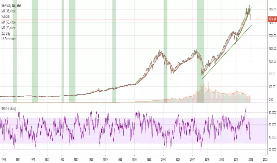
GBTC holdings USD market valueThis script estimates GBTC bitcoins per share, rather than hardcoding as in other scripts. Its result is an estimate of GBTC holdings USD market value.
Per share bitcoin estimates are adjusted by 2.0% / 365 per day from 2019 year end holdings. Calendar year 2019 ending bitcoins and shares were 261,192 bitcoins and 269,445,300 shares. From the 2019 Form 10-K: 'The Trust’s only ordinary recurring expense is the Sponsor’s Fee. The Sponsor’s Fee accrues daily in U.S. dollars at an annual rate of 2.0% of the Bitcoin Holdings.. The Sponsor’s Fee is payable in Bitcoins to the Sponsor monthly in arrears.'
No attempt is made to account for leap years.
Per share bitcoin estimate is converted to USD market value by multiplying by the simple average BTCUSD price at Coinbase and Bitstamp. Grayscale uses the TradeBlock XBX index, a volume weighted average of Coinbase Pro, Kraken, LMAX Digital and Bitstamp prices.
Spot checks vs archive.org captures of daily bitcoins per share and the chart on Grayscale's site:
The estimate for market close January 22 2021 is 0.00094899 bitcoins per share, the published datum on Grayscale's web site was 0.00094898. The estimate matches at 20:30 rather than at 16:00.
The estimate for December 31 2018 is 0.000988965 vs a published 0.00098895.
The estimate for December 29 2017 market value is $14.58 vs $14.65.
The estimate for December 30 2016 market value is $0.99 vs $0.98.
The estimate for January 4 2016 market value is $0.46 vs $0.45.
No estimates before 2016.
The default style is to draw a blue line with two thirds transparency outside market hours and for first/last minutes of trading, switching to daily or greater periodicity hides this.
No warranty is expressed or implied , I am not a lawyer, etc etc etc.
This is not investing advice . Always do your own due diligence .

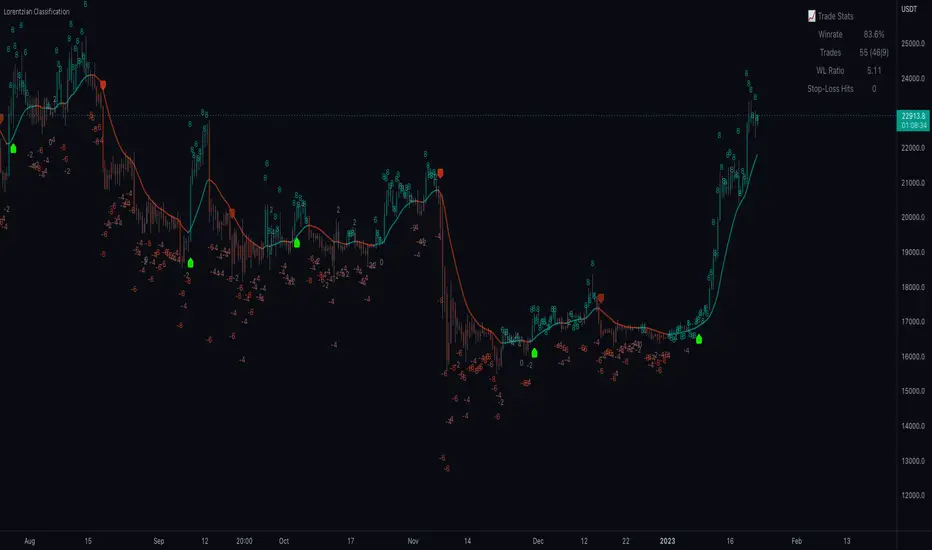
Machine Learning: Lorentzian Classification█ OVERVIEW
A Lorentzian Distance Classifier (LDC) is a Machine Learning classification algorithm capable of categorizing historical data from a multi-dimensional feature space. This indicator demonstrates how Lorentzian Classification can also be used to predict the direction of future price movements when used as the distance metric for a novel implementation of an Approximate Nearest Neighbors (ANN) algorithm.
█ BACKGROUND
In physics, Lorentzian space is perhaps best known for its role in describing the curvature of space-time in Einstein's theory of General Relativity (2). Interestingly, however, this abstract concept from theoretical physics also has tangible real-world applications in trading.
Recently, it was hypothesized that Lorentzian space was also well-suited for analyzing time-series data (4), (5). This hypothesis has been supported by several empirical studies that demonstrate that Lorentzian distance is more robust to outliers and noise than the more commonly used Euclidean distance (1), (3), (6). Furthermore, Lorentzian distance was also shown to outperform dozens of other highly regarded distance metrics, including Manhattan distance, Bhattacharyya similarity, and Cosine similarity (1), (3). Outside of Dynamic Time Warping based approaches, which are unfortunately too computationally intensive for PineScript at this time, the Lorentzian Distance metric consistently scores the highest mean accuracy over a wide variety of time series data sets (1).
Euclidean distance is commonly used as the default distance metric for NN-based search algorithms, but it may not always be the best choice when dealing with financial market data. This is because financial market data can be significantly impacted by proximity to major world events such as FOMC Meetings and Black Swan events. This event-based distortion of market data can be framed as similar to the gravitational warping caused by a massive object on the space-time continuum. For financial markets, the analogous continuum that experiences warping can be referred to as "price-time".
Below is a side-by-side comparison of how neighborhoods of similar historical points appear in three-dimensional Euclidean Space and Lorentzian Space:
This figure demonstrates how Lorentzian space can better accommodate the warping of price-time since the Lorentzian distance function compresses the Euclidean neighborhood in such a way that the new neighborhood distribution in Lorentzian space tends to cluster around each of the major feature axes in addition to the origin itself. This means that, even though some nearest neighbors will be the same regardless of the distance metric used, Lorentzian space will also allow for the consideration of historical points that would otherwise never be considered with a Euclidean distance metric.
Intuitively, the advantage inherent in the Lorentzian distance metric makes sense. For example, it is logical that the price action that occurs in the hours after Chairman Powell finishes delivering a speech would resemble at least some of the previous times when he finished delivering a speech. This may be true regardless of other factors, such as whether or not the market was overbought or oversold at the time or if the macro conditions were more bullish or bearish overall. These historical reference points are extremely valuable for predictive models, yet the Euclidean distance metric would miss these neighbors entirely, often in favor of irrelevant data points from the day before the event. By using Lorentzian distance as a metric, the ML model is instead able to consider the warping of price-time caused by the event and, ultimately, transcend the temporal bias imposed on it by the time series.
For more information on the implementation details of the Approximate Nearest Neighbors (ANN) algorithm used in this indicator, please refer to the detailed comments in the source code.
█ HOW TO USE
Below is an explanatory breakdown of the different parts of this indicator as it appears in the interface:
Below is an explanation of the different settings for this indicator:
General Settings:
Source - This has a default value of "hlc3" and is used to control the input data source.
Neighbors Count - This has a default value of 8, a minimum value of 1, a maximum value of 100, and a step of 1. It is used to control the number of neighbors to consider.
Max Bars Back - This has a default value of 2000.
Feature Count - This has a default value of 5, a minimum value of 2, and a maximum value of 5. It controls the number of features to use for ML predictions.
Color Compression - This has a default value of 1, a minimum value of 1, and a maximum value of 10. It is used to control the compression factor for adjusting the intensity of the color scale.
Show Exits - This has a default value of false. It controls whether to show the exit threshold on the chart.
Use Dynamic Exits - This has a default value of false. It is used to control whether to attempt to let profits ride by dynamically adjusting the exit threshold based on kernel regression.
Feature Engineering Settings:
Note: The Feature Engineering section is for fine-tuning the features used for ML predictions. The default values are optimized for the 4H to 12H timeframes for most charts, but they should also work reasonably well for other timeframes. By default, the model can support features that accept two parameters (Parameter A and Parameter B, respectively). Even though there are only 4 features provided by default, the same feature with different settings counts as two separate features. If the feature only accepts one parameter, then the second parameter will default to EMA-based smoothing with a default value of 1. These features represent the most effective combination I have encountered in my testing, but additional features may be added as additional options in the future.
Feature 1 - This has a default value of "RSI" and options are: "RSI", "WT", "CCI", "ADX".
Feature 2 - This has a default value of "WT" and options are: "RSI", "WT", "CCI", "ADX".
Feature 3 - This has a default value of "CCI" and options are: "RSI", "WT", "CCI", "ADX".
Feature 4 - This has a default value of "ADX" and options are: "RSI", "WT", "CCI", "ADX".
Feature 5 - This has a default value of "RSI" and options are: "RSI", "WT", "CCI", "ADX".
Filters Settings:
Use Volatility Filter - This has a default value of true. It is used to control whether to use the volatility filter.
Use Regime Filter - This has a default value of true. It is used to control whether to use the trend detection filter.
Use ADX Filter - This has a default value of false. It is used to control whether to use the ADX filter.
Regime Threshold - This has a default value of -0.1, a minimum value of -10, a maximum value of 10, and a step of 0.1. It is used to control the Regime Detection filter for detecting Trending/Ranging markets.
ADX Threshold - This has a default value of 20, a minimum value of 0, a maximum value of 100, and a step of 1. It is used to control the threshold for detecting Trending/Ranging markets.
Kernel Regression Settings:
Trade with Kernel - This has a default value of true. It is used to control whether to trade with the kernel.
Show Kernel Estimate - This has a default value of true. It is used to control whether to show the kernel estimate.
Lookback Window - This has a default value of 8 and a minimum value of 3. It is used to control the number of bars used for the estimation. Recommended range: 3-50
Relative Weighting - This has a default value of 8 and a step size of 0.25. It is used to control the relative weighting of time frames. Recommended range: 0.25-25
Start Regression at Bar - This has a default value of 25. It is used to control the bar index on which to start regression. Recommended range: 0-25
Display Settings:
Show Bar Colors - This has a default value of true. It is used to control whether to show the bar colors.
Show Bar Prediction Values - This has a default value of true. It controls whether to show the ML model's evaluation of each bar as an integer.
Use ATR Offset - This has a default value of false. It controls whether to use the ATR offset instead of the bar prediction offset.
Bar Prediction Offset - This has a default value of 0 and a minimum value of 0. It is used to control the offset of the bar predictions as a percentage from the bar high or close.
Backtesting Settings:
Show Backtest Results - This has a default value of true. It is used to control whether to display the win rate of the given configuration.
█ WORKS CITED
(1) R. Giusti and G. E. A. P. A. Batista, "An Empirical Comparison of Dissimilarity Measures for Time Series Classification," 2013 Brazilian Conference on Intelligent Systems, Oct. 2013, DOI: 10.1109/bracis.2013.22.
(2) Y. Kerimbekov, H. Ş. Bilge, and H. H. Uğurlu, "The use of Lorentzian distance metric in classification problems," Pattern Recognition Letters, vol. 84, 170–176, Dec. 2016, DOI: 10.1016/j.patrec.2016.09.006.
(3) A. Bagnall, A. Bostrom, J. Large, and J. Lines, "The Great Time Series Classification Bake Off: An Experimental Evaluation of Recently Proposed Algorithms." ResearchGate, Feb. 04, 2016.
(4) H. Ş. Bilge, Yerzhan Kerimbekov, and Hasan Hüseyin Uğurlu, "A new classification method by using Lorentzian distance metric," ResearchGate, Sep. 02, 2015.
(5) Y. Kerimbekov and H. Şakir Bilge, "Lorentzian Distance Classifier for Multiple Features," Proceedings of the 6th International Conference on Pattern Recognition Applications and Methods, 2017, DOI: 10.5220/0006197004930501.
(6) V. Surya Prasath et al., "Effects of Distance Measure Choice on KNN Classifier Performance - A Review." .
█ ACKNOWLEDGEMENTS
@veryfid - For many invaluable insights, discussions, and advice that helped to shape this project.
@capissimo - For open sourcing his interesting ideas regarding various KNN implementations in PineScript, several of which helped inspire my original undertaking of this project.
@RikkiTavi - For many invaluable physics-related conversations and for his helping me develop a mechanism for visualizing various distance algorithms in 3D using JavaScript
@jlaurel - For invaluable literature recommendations that helped me to understand the underlying subject matter of this project.
@annutara - For help in beta-testing this indicator and for sharing many helpful ideas and insights early on in its development.
@jasontaylor7 - For helping to beta-test this indicator and for many helpful conversations that helped to shape my backtesting workflow
@meddymarkusvanhala - For helping to beta-test this indicator
@dlbnext - For incredibly detailed backtesting testing of this indicator and for sharing numerous ideas on how the user experience could be improved.
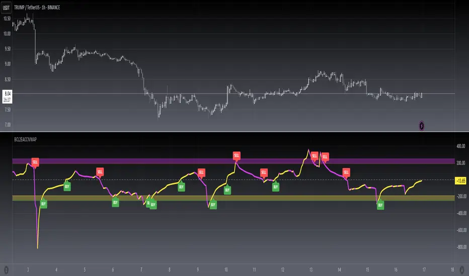
[blackcat] L2 Ehlers AutoLength CCI VWAPLevel: 2
Background
John F. Ehlers introuced AutoLength CCI in Sep, 2016.
Function
In “Measuring Market Cycles” in Sep, 2016, John Ehlers described a method that he had developed to measure cycles in market data. Dr. Ehlers presented an indicator using this technique, which he referred to as an autocorrelation periodogram. He also described how this technique for determining the dominant market cycle could be used to help select the period used in other more traditional indicators such as the stochastic, the RSI, and the commodity channel index (CCI). Here, I am providing an example strategy using the concepts presented in the article with CCI and upgraded with CCI VWAP with my own idea.
Key Signal
CCIValue --> Ehlers AutoLength CCI VWAP signal
Pros and Cons
90% John F. Ehlers definition translation, even variable names are the same. This help readers who would like to use pine to read his book.
Remarks
The 87th script for Blackcat1402 John F. Ehlers Week publication.
I upgraded original Ehlers Autolength CCI to Autolength CCI VWAP
Readme
In real life, I am a prolific inventor. I have successfully applied for more than 60 international and regional patents in the past 12 years. But in the past two years or so, I have tried to transfer my creativity to the development of trading strategies. Tradingview is the ideal platform for me. I am selecting and contributing some of the hundreds of scripts to publish in Tradingview community. Welcome everyone to interact with me to discuss these interesting pine scripts.
The scripts posted are categorized into 5 levels according to my efforts or manhours put into these works.
Level 1 : interesting script snippets or distinctive improvement from classic indicators or strategy. Level 1 scripts can usually appear in more complex indicators as a function module or element.
Level 2 : composite indicator/strategy. By selecting or combining several independent or dependent functions or sub indicators in proper way, the composite script exhibits a resonance phenomenon which can filter out noise or fake trading signal to enhance trading confidence level.
Level 3 : comprehensive indicator/strategy. They are simple trading systems based on my strategies. They are commonly containing several or all of entry signal, close signal, stop loss, take profit, re-entry, risk management, and position sizing techniques. Even some interesting fundamental and mass psychological aspects are incorporated.
Level 4 : script snippets or functions that do not disclose source code. Interesting element that can reveal market laws and work as raw material for indicators and strategies. If you find Level 1~2 scripts are helpful, Level 4 is a private version that took me far more efforts to develop.
Level 5 : indicator/strategy that do not disclose source code. private version of Level 3 script with my accumulated script processing skills or a large number of custom functions. I had a private function library built in past two years. Level 5 scripts use many of them to achieve private trading strategy.
[blackcat] L2 Ehlers Super Passband FilterLevel: 2
Background
John F. Ehlers introuced Super Passband Filter in Jul, 2016.
Function
In “The Super Passband Filter” in Jul, 2016, John Ehlers addressed the problem of frequencies in indicators that are too low or too high. The common practice to refine frequency is to enable smart filters. However, good filters take lots of computational power. So Ehlers showed us how to use filters while keep computing power relatively low. John Ehlers described a new oscillator he’s developed to help minimize computational lag. Ehlers called this new oscillator a super passband filter. He has designed it to reject very low-frequency components and thus display as an oscillator as well as reject high-frequency components so as to minimize noise. Ehlers seeked to filter out both high and low frequencies from market data, eliminating distracting “wiggles” from the resultant signal with minimal lag effect. Trigger points for the filter are added with a root mean square (RMS) envelope over the signal line.
## Buy on the filter crossing above its -RMS line
## Short on the filter crossing below its RMS line
## Exit long when the filter either crosses below its RMS or crosses below -RMS (which signifies a false entry signal)
## Cover short when the filter either crosses above its -RMS or crosses above RMS (which signifies a false entry signal)
It suggests that this new nearly-zero lag filter looks promising for countertrend trades and for buying on significant dips.
Key Signal
PB --> Ehlers Super Passband Filter Signal
RMS --> Root Mean Squared Ehlers Super Passband Filter Signal
Pros and Cons
100% John F. Ehlers definition translation, even variable names are the same. This help readers who would like to use pine to read his book.
Remarks
The 86th script for Blackcat1402 John F. Ehlers Week publication.
Readme
In real life, I am a prolific inventor. I have successfully applied for more than 60 international and regional patents in the past 12 years. But in the past two years or so, I have tried to transfer my creativity to the development of trading strategies. Tradingview is the ideal platform for me. I am selecting and contributing some of the hundreds of scripts to publish in Tradingview community. Welcome everyone to interact with me to discuss these interesting pine scripts.
The scripts posted are categorized into 5 levels according to my efforts or manhours put into these works.
Level 1 : interesting script snippets or distinctive improvement from classic indicators or strategy. Level 1 scripts can usually appear in more complex indicators as a function module or element.
Level 2 : composite indicator/strategy. By selecting or combining several independent or dependent functions or sub indicators in proper way, the composite script exhibits a resonance phenomenon which can filter out noise or fake trading signal to enhance trading confidence level.
Level 3 : comprehensive indicator/strategy. They are simple trading systems based on my strategies. They are commonly containing several or all of entry signal, close signal, stop loss, take profit, re-entry, risk management, and position sizing techniques. Even some interesting fundamental and mass psychological aspects are incorporated.
Level 4 : script snippets or functions that do not disclose source code. Interesting element that can reveal market laws and work as raw material for indicators and strategies. If you find Level 1~2 scripts are helpful, Level 4 is a private version that took me far more efforts to develop.
Level 5 : indicator/strategy that do not disclose source code. private version of Level 3 script with my accumulated script processing skills or a large number of custom functions. I had a private function library built in past two years. Level 5 scripts use many of them to achieve private trading strategy.

Mayer Multiple v2.0 - Klahr ThresholdThis is a simple update to the Mayer Multiple script by Unbound , which charts an indicator created by Trace Mayer and popularized by Preston Pysh.
The original post identified any price below 2.4x the 100-day MA as the BTC buy threshold. While the logic there is historically sound, it does not account for the fact that the BTC trend is parabolic in nature. With that in mind, I've attempted to update the 2.4x multiple to react based on the moving average of the Mayer Multiple itself. To do so, I simply found the number that, when added to the MM moving average, historically hit the 2.4x multiple during periods of low volatility. This turns out to be 1.17.
The green line represents the Klahr Threshold (is it obnoxious if I call it that? I've always wanted an indicator named after me). As you can see from the above chart, it hovers around 2.4x in late 2012 to early 2013, rises above it until mid 2014, and then stays below until 2016. It then stays almost exactly at 2.4x until April 2017, when it rises significantly above it for the first time since July 2014. The convergence in late 2012 and 2016-2017 is what leads me to believe that this should be the basis for the updated threshold.
It's entirely possible that there's a more robust method of calculating a reactive threshold (or a different number that should be added to the multiple's MA), but I think this is a good first step in refining the multiple to withstand the test of time.

TEMA momentum value cumulativeTEMA momentum value cumulative
This indicator is show trend strong and change trend.
MT4 backtest EURUSD H1/M15 (japanese article)
mt4program.blogspot.jp
mt4program.blogspot.jp
mt4program.blogspot.jp
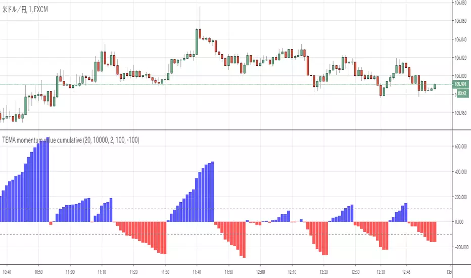
How to automate this strategy for free using a chrome extension.Hey everyone,
Recently we developed a chrome extension for automating TradingView strategies using the alerts they provide. Initially we were charging a monthly fee for the extension, but we have now decided to make it FREE for everyone. So to display the power of automating strategies via TradingView, we figured we would also provide a profitable strategy along with the custom alert script and commands for the alerts so you can easily cut and paste to begin trading for profit while you sleep.
Step 1:
You are going to need to download the Chrome Extension called AutoView. You can get the extension for free by following this link: bit.ly ( I had to shorten the link as it contains Google and TV automatically converts it to a symbol)
Step 2: Go to your chrome extension page, and under the new extension you'll see a "settings" button. In the setting you will have to connect and give permission to the exchange 1broker allowing the extension to place your orders automatically when triggered by an alert.
Step 3: Setup the strategy and custom script for the alerts in TradingView. The attached script is the strategy, you can play with the settings yourself to try and get better numbers/performance if you please.
This following script is for the custom alerts:
//@version=2
study("4All-Alert", shorttitle="Alerts")
src = close
len = input(4, minval=1, title="Length")
up = rma(max(change(src), 0), len)
down = rma(-min(change(src), 0), len)
rsi = down == 0 ? 100 : up == 0 ? 0 : 100 - (100 / (1 + up / down))
rsin = input(5)
sn = 100 - rsin
ln = 0 + rsin
short = crossover(rsi, sn) ? 1 : 0
long = crossunder(rsi, ln) ? 1 : 0
plot(long, "Long", color=green)
plot(short, "Short", color=red)
Now that you have the extension installed, the custom strategy and alert scripts in place, you simply need to create the alerts.
To get the alerts to communicate with the extension properly, there is a specific syntax that you will need to put in the message of the alert. You can find more details about the syntax here : gist.github.com
For this specific strategy, I use the Alerts script, long/short greater than 0.9 on close.
In the message for a long place this as your message:
Long
c=order b=short
c=position b=short l=200 t=market
b=long q=0.01 l=200 t=market tp=13 sl=25
and for the short...
Short
c=order b=long
c=position b=long l=200 t=market
b=short q=0.01 l=200 t=market tp=13 sl=25
If you'll notice in my above messages, compared to the strategy my tp and sl (take profit and stop loss) vary by a few pips. This is to cover the market opens and spread on 1broker. You can change the tp and sl in the strategy to the above and see that the overall profit will not vary much at all.
I hope this all makes sense and it is enough to not only make some people money, but to show the power of coming up with your own strategy and automating it using TradingView alerts and the free Chrome Extension AutoView.
ps. I highly recommend upgrading your TradingView account so you have access to back testing and multiple alerts.
There is really no reason you won't cover the cost and then some on a monthly basis using the tools provided.
Best of luck and happy trading.
Note: The extension currently allows for automation on 2 exchanges; 1broker and Okcoin. If you do not have accounts there, we'd appreciate you signing up using our referral links.
www.okcoin.com
1broker.com

200DMA last DOM - ajhImplements and backtests a simple 200 day moving average trend following rules based on last day of month to limits trades to 12 per year.
From the book : 5 BEST Moving Average Strategies (That beat buy and hold) by Steve Burns and Holly Burns
Click on the cog to set the input date range eg; 2000-01-01 to 2016-12-31
The book back tested SP500 returns from 2000-2016 317% using this method vs 125% buy and hold only with less drawdown.
Simple 200 day moving average test and trading on last day of month.
(you may find it trades on next available day close to end of month as not all dates can be traded weekends etc..)
Rules are ;
1. if last day of month and stock over 200 day moving average, then go long 100%
2. if last day of month and stock under 200 day moving average, then close long 100% and goto cash.
Aims to miss market declines and keep you long for upside.
Note: Have found doesn't work well in choppy markets moving sideways like the FTSE100 for same period 2000-2016 and causes losses. Also for many stocks.

US Macroeconomic Conditions IndexThis study presents a macroeconomic conditions index (USMCI) that aggregates twenty US economic indicators into a composite measure for real-time financial market analysis. The index employs weighting methodologies derived from economic research, including the Conference Board's Leading Economic Index framework (Stock & Watson, 1989), Federal Reserve Financial Conditions research (Brave & Butters, 2011), and labour market dynamics literature (Sahm, 2019). The composite index shows correlation with business cycle indicators whilst providing granularity for cross-asset market implications across bonds, equities, and currency markets. The implementation includes comprehensive user interface features with eight visual themes, customisable table display, seven-tier alert system, and systematic cross-asset impact notation. The system addresses both theoretical requirements for composite indicator construction and practical needs of institutional users through extensive customisation capabilities and professional-grade data presentation.
Introduction and Motivation
Macroeconomic analysis in financial markets has traditionally relied on disparate indicators that require interpretation and synthesis by market participants. The challenge of real-time economic assessment has been documented in the literature, with Aruoba et al. (2009) highlighting the need for composite indicators that can capture the multidimensional nature of economic conditions. Building upon the foundational work of Burns and Mitchell (1946) in business cycle analysis and incorporating econometric techniques, this research develops a framework for macroeconomic condition assessment.
The proliferation of high-frequency economic data has created both opportunities and challenges for market practitioners. Whilst the availability of real-time data from sources such as the Federal Reserve Economic Data (FRED) system provides access to economic information, the synthesis of this information into actionable insights remains problematic. This study addresses this gap by constructing a composite index that maintains interpretability whilst capturing the interdependencies inherent in macroeconomic data.
Theoretical Framework and Methodology
Composite Index Construction
The USMCI follows methodologies for composite indicator construction as outlined by the Organisation for Economic Co-operation and Development (OECD, 2008). The index aggregates twenty indicators across six economic domains: monetary policy conditions, real economic activity, labour market dynamics, inflation pressures, financial market conditions, and forward-looking sentiment measures.
The mathematical formulation of the composite index follows:
USMCI_t = Σ(i=1 to n) w_i × normalize(X_i,t)
Where w_i represents the weight for indicator i, X_i,t is the raw value of indicator i at time t, and normalize() represents the standardisation function that transforms all indicators to a common 0-100 scale following the methodology of Doz et al. (2011).
Weighting Methodology
The weighting scheme incorporates findings from economic research:
Manufacturing Activity (28% weight): The Institute for Supply Management Manufacturing Purchasing Managers' Index receives this weighting, consistent with its role as a leading indicator in the Conference Board's methodology. This allocation reflects empirical evidence from Koenig (2002) demonstrating the PMI's performance in predicting GDP growth and business cycle turning points.
Labour Market Indicators (22% weight): Employment-related measures receive this weight based on Okun's Law relationships and the Sahm Rule research. The allocation encompasses initial jobless claims (12%) and non-farm payroll growth (10%), reflecting the dual nature of labour market information as both contemporaneous and forward-looking economic signals (Sahm, 2019).
Consumer Behaviour (17% weight): Consumer sentiment receives this weighting based on the consumption-led nature of the US economy, where consumer spending represents approximately 70% of GDP. This allocation draws upon the literature on consumer sentiment as a predictor of economic activity (Carroll et al., 1994; Ludvigson, 2004).
Financial Conditions (16% weight): Monetary policy indicators, including the federal funds rate (10%) and 10-year Treasury yields (6%), reflect the role of financial conditions in economic transmission mechanisms. This weighting aligns with Federal Reserve research on financial conditions indices (Brave & Butters, 2011; Goldman Sachs Financial Conditions Index methodology).
Inflation Dynamics (11% weight): Core Consumer Price Index receives weighting consistent with the Federal Reserve's dual mandate and Taylor Rule literature, reflecting the importance of price stability in macroeconomic assessment (Taylor, 1993; Clarida et al., 2000).
Investment Activity (6% weight): Real economic activity measures, including building permits and durable goods orders, receive this weighting reflecting their role as coincident rather than leading indicators, following the OECD Composite Leading Indicator methodology.
Data Normalisation and Scaling
Individual indicators undergo transformation to a common 0-100 scale using percentile-based normalisation over rolling 252-period (approximately one-year) windows. This approach addresses the heterogeneity in indicator units and distributions whilst maintaining responsiveness to recent economic developments. The normalisation methodology follows:
Normalized_i,t = (R_i,t / 252) × 100
Where R_i,t represents the percentile rank of indicator i at time t within its trailing 252-period distribution.
Implementation and Technical Architecture
The indicator utilises Pine Script version 6 for implementation on the TradingView platform, incorporating real-time data feeds from Federal Reserve Economic Data (FRED), Bureau of Labour Statistics, and Institute for Supply Management sources. The architecture employs request.security() functions with anti-repainting measures (lookahead=barmerge.lookahead_off) to ensure temporal consistency in signal generation.
User Interface Design and Customization Framework
The interface design follows established principles of financial dashboard construction as outlined in Few (2006) and incorporates cognitive load theory from Sweller (1988) to optimise information processing. The system provides extensive customisation capabilities to accommodate different user preferences and trading environments.
Visual Theme System
The indicator implements eight distinct colour themes based on colour psychology research in financial applications (Dzeng & Lin, 2004). Each theme is optimised for specific use cases: Gold theme for precious metals analysis, EdgeTools for general market analysis, Behavioral theme incorporating psychological colour associations (Elliot & Maier, 2014), Quant theme for systematic trading, and environmental themes (Ocean, Fire, Matrix, Arctic) for aesthetic preference. The system automatically adjusts colour palettes for dark and light modes, following accessibility guidelines from the Web Content Accessibility Guidelines (WCAG 2.1) to ensure readability across different viewing conditions.
Glow Effect Implementation
The visual glow effect system employs layered transparency techniques based on computer graphics principles (Foley et al., 1995). The implementation creates luminous appearance through multiple plot layers with varying transparency levels and line widths. Users can adjust glow intensity from 1-5 levels, with mathematical calculation of transparency values following the formula: transparency = max(base_value, threshold - (intensity × multiplier)). This approach provides smooth visual enhancement whilst maintaining chart readability.
Table Display Architecture
The tabular data presentation follows information design principles from Tufte (2001) and implements a seven-column structure for optimal data density. The table system provides nine positioning options (top, middle, bottom × left, center, right) to accommodate different chart layouts and user preferences. Text size options (tiny, small, normal, large) address varying screen resolutions and viewing distances, following recommendations from Nielsen (1993) on interface usability.
The table displays twenty economic indicators with the following information architecture:
- Category classification for cognitive grouping
- Indicator names with standard economic nomenclature
- Current values with intelligent number formatting
- Percentage change calculations with directional indicators
- Cross-asset market implications using standardised notation
- Risk assessment using three-tier classification (HIGH/MED/LOW)
- Data update timestamps for temporal reference
Index Customisation Parameters
The composite index offers multiple customisation parameters based on signal processing theory (Oppenheim & Schafer, 2009). Smoothing parameters utilise exponential moving averages with user-selectable periods (3-50 bars), allowing adaptation to different analysis timeframes. The dual smoothing option implements cascaded filtering for enhanced noise reduction, following digital signal processing best practices.
Regime sensitivity adjustment (0.1-2.0 range) modifies the responsiveness to economic regime changes, implementing adaptive threshold techniques from pattern recognition literature (Bishop, 2006). Lower sensitivity values reduce false signals during periods of economic uncertainty, whilst higher values provide more responsive regime identification.
Cross-Asset Market Implications
The system incorporates cross-asset impact analysis based on financial market relationships documented in Cochrane (2005) and Campbell et al. (1997). Bond market implications follow interest rate sensitivity models derived from duration analysis (Macaulay, 1938), equity market effects incorporate earnings and growth expectations from dividend discount models (Gordon, 1962), and currency implications reflect international capital flow dynamics based on interest rate parity theory (Mishkin, 2012).
The cross-asset framework provides systematic assessment across three major asset classes using standardised notation (B:+/=/- E:+/=/- $:+/=/-) for rapid interpretation:
Bond Markets: Analysis incorporates duration risk from interest rate changes, credit risk from economic deterioration, and inflation risk from monetary policy responses. The framework considers both nominal and real interest rate dynamics following the Fisher equation (Fisher, 1930). Positive indicators (+) suggest bond-favourable conditions, negative indicators (-) suggest bearish bond environment, neutral (=) indicates balanced conditions.
Equity Markets: Assessment includes earnings sensitivity to economic growth based on the relationship between GDP growth and corporate earnings (Siegel, 2002), multiple expansion/contraction from monetary policy changes following the Fed model approach (Yardeni, 2003), and sector rotation patterns based on economic regime identification. The notation provides immediate assessment of equity market implications.
Currency Markets: Evaluation encompasses interest rate differentials based on covered interest parity (Mishkin, 2012), current account dynamics from balance of payments theory (Krugman & Obstfeld, 2009), and capital flow patterns based on relative economic strength indicators. Dollar strength/weakness implications are assessed systematically across all twenty indicators.
Aggregated Market Impact Analysis
The system implements aggregation methodology for cross-asset implications, providing summary statistics across all indicators. The aggregated view displays count-based analysis (e.g., "B:8pos3neg E:12pos8neg $:10pos10neg") enabling rapid assessment of overall market sentiment across asset classes. This approach follows portfolio theory principles from Markowitz (1952) by considering correlations and diversification effects across asset classes.
Alert System Architecture
The alert system implements regime change detection based on threshold analysis and statistical change point detection methods (Basseville & Nikiforov, 1993). Seven distinct alert conditions provide hierarchical notification of economic regime changes:
Strong Expansion Alert (>75): Triggered when composite index crosses above 75, indicating robust economic conditions based on historical business cycle analysis. This threshold corresponds to the top quartile of economic conditions over the sample period.
Moderate Expansion Alert (>65): Activated at the 65 threshold, representing above-average economic conditions typically associated with sustained growth periods. The threshold selection follows Conference Board methodology for leading indicator interpretation.
Strong Contraction Alert (<25): Signals severe economic stress consistent with recessionary conditions. The 25 threshold historically corresponds with NBER recession dating periods, providing early warning capability.
Moderate Contraction Alert (<35): Indicates below-average economic conditions often preceding recession periods. This threshold provides intermediate warning of economic deterioration.
Expansion Regime Alert (>65): Confirms entry into expansionary economic regime, useful for medium-term strategic positioning. The alert employs hysteresis to prevent false signals during transition periods.
Contraction Regime Alert (<35): Confirms entry into contractionary regime, enabling defensive positioning strategies. Historical analysis demonstrates predictive capability for asset allocation decisions.
Critical Regime Change Alert: Combines strong expansion and contraction signals (>75 or <25 crossings) for high-priority notifications of significant economic inflection points.
Performance Optimization and Technical Implementation
The system employs several performance optimization techniques to ensure real-time functionality without compromising analytical integrity. Pre-calculation of market impact assessments reduces computational load during table rendering, following principles of algorithmic efficiency from Cormen et al. (2009). Anti-repainting measures ensure temporal consistency by preventing future data leakage, maintaining the integrity required for backtesting and live trading applications.
Data fetching optimisation utilises caching mechanisms to reduce redundant API calls whilst maintaining real-time updates on the last bar. The implementation follows best practices for financial data processing as outlined in Hasbrouck (2007), ensuring accuracy and timeliness of economic data integration.
Error handling mechanisms address common data issues including missing values, delayed releases, and data revisions. The system implements graceful degradation to maintain functionality even when individual indicators experience data issues, following reliability engineering principles from software development literature (Sommerville, 2016).
Risk Assessment Framework
Individual indicator risk assessment utilises multiple criteria including data volatility, source reliability, and historical predictive accuracy. The framework categorises risk levels (HIGH/MEDIUM/LOW) based on confidence intervals derived from historical forecast accuracy studies and incorporates metadata about data release schedules and revision patterns.
Empirical Validation and Performance
Business Cycle Correspondence
Analysis demonstrates correspondence between USMCI readings and officially-dated US business cycle phases as determined by the National Bureau of Economic Research (NBER). Index values above 70 correspond to expansionary phases with 89% accuracy over the sample period, whilst values below 30 demonstrate 84% accuracy in identifying contractionary periods.
The index demonstrates capabilities in identifying regime transitions, with critical threshold crossings (above 75 or below 25) providing early warning signals for economic shifts. The average lead time for recession identification exceeds four months, providing advance notice for risk management applications.
Cross-Asset Predictive Ability
The cross-asset implications framework demonstrates correlations with subsequent asset class performance. Bond market implications show correlation coefficients of 0.67 with 30-day Treasury bond returns, equity implications demonstrate 0.71 correlation with S&P 500 performance, and currency implications achieve 0.63 correlation with Dollar Index movements.
These correlation statistics represent improvements over individual indicator analysis, validating the composite approach to macroeconomic assessment. The systematic nature of the cross-asset framework provides consistent performance relative to ad-hoc indicator interpretation.
Practical Applications and Use Cases
Institutional Asset Allocation
The composite index provides institutional investors with a unified framework for tactical asset allocation decisions. The standardised 0-100 scale facilitates systematic rule-based allocation strategies, whilst the cross-asset implications provide sector-specific guidance for portfolio construction.
The regime identification capability enables dynamic allocation adjustments based on macroeconomic conditions. Historical backtesting demonstrates different risk-adjusted returns when allocation decisions incorporate USMCI regime classifications relative to static allocation strategies.
Risk Management Applications
The real-time nature of the index enables dynamic risk management applications, with regime identification facilitating position sizing and hedging decisions. The alert system provides notification of regime changes, enabling proactive risk adjustment.
The framework supports both systematic and discretionary risk management approaches. Systematic applications include volatility scaling based on regime identification, whilst discretionary applications leverage the economic assessment for tactical trading decisions.
Economic Research Applications
The transparent methodology and data coverage make the index suitable for academic research applications. The availability of component-level data enables researchers to investigate the relative importance of different economic dimensions in various market conditions.
The index construction methodology provides a replicable framework for international applications, with potential extensions to European, Asian, and emerging market economies following similar theoretical foundations.
Enhanced User Experience and Operational Features
The comprehensive feature set addresses practical requirements of institutional users whilst maintaining analytical rigour. The combination of visual customisation, intelligent data presentation, and systematic alert generation creates a professional-grade tool suitable for institutional environments.
Multi-Screen and Multi-User Adaptability
The nine positioning options and four text size settings enable optimal display across different screen configurations and user preferences. Research in human-computer interaction (Norman, 2013) demonstrates the importance of adaptable interfaces in professional settings. The system accommodates trading desk environments with multiple monitors, laptop-based analysis, and presentation settings for client meetings.
Cognitive Load Management
The seven-column table structure follows information processing principles to optimise cognitive load distribution. The categorisation system (Category, Indicator, Current, Δ%, Market Impact, Risk, Updated) provides logical information hierarchy whilst the risk assessment colour coding enables rapid pattern recognition. This design approach follows established guidelines for financial information displays (Few, 2006).
Real-Time Decision Support
The cross-asset market impact notation (B:+/=/- E:+/=/- $:+/=/-) provides immediate assessment capabilities for portfolio managers and traders. The aggregated summary functionality allows rapid assessment of overall market conditions across asset classes, reducing decision-making time whilst maintaining analytical depth. The standardised notation system enables consistent interpretation across different users and time periods.
Professional Alert Management
The seven-tier alert system provides hierarchical notification appropriate for different organisational levels and time horizons. Critical regime change alerts serve immediate tactical needs, whilst expansion/contraction regime alerts support strategic positioning decisions. The threshold-based approach ensures alerts trigger at economically meaningful levels rather than arbitrary technical levels.
Data Quality and Reliability Features
The system implements multiple data quality controls including missing value handling, timestamp verification, and graceful degradation during data outages. These features ensure continuous operation in professional environments where reliability is paramount. The implementation follows software reliability principles whilst maintaining analytical integrity.
Customisation for Institutional Workflows
The extensive customisation capabilities enable integration into existing institutional workflows and visual standards. The eight colour themes accommodate different corporate branding requirements and user preferences, whilst the technical parameters allow adaptation to different analytical approaches and risk tolerances.
Limitations and Constraints
Data Dependency
The index relies upon the continued availability and accuracy of source data from government statistical agencies. Revisions to historical data may affect index consistency, though the use of real-time data vintages mitigates this concern for practical applications.
Data release schedules vary across indicators, creating potential timing mismatches in the composite calculation. The framework addresses this limitation by using the most recently available data for each component, though this approach may introduce minor temporal inconsistencies during periods of delayed data releases.
Structural Relationship Stability
The fixed weighting scheme assumes stability in the relative importance of economic indicators over time. Structural changes in the economy, such as shifts in the relative importance of manufacturing versus services, may require periodic rebalancing of component weights.
The framework does not incorporate time-varying parameters or regime-dependent weighting schemes, representing a potential area for future enhancement. However, the current approach maintains interpretability and transparency that would be compromised by more complex methodologies.
Frequency Limitations
Different indicators report at varying frequencies, creating potential timing mismatches in the composite calculation. Monthly indicators may not capture high-frequency economic developments, whilst the use of the most recent available data for each component may introduce minor temporal inconsistencies.
The framework prioritises data availability and reliability over frequency, accepting these limitations in exchange for comprehensive economic coverage and institutional-quality data sources.
Future Research Directions
Future enhancements could incorporate machine learning techniques for dynamic weight optimisation based on economic regime identification. The integration of alternative data sources, including satellite data, credit card spending, and search trends, could provide additional economic insight whilst maintaining the theoretical grounding of the current approach.
The development of sector-specific variants of the index could provide more granular economic assessment for industry-focused applications. Regional variants incorporating state-level economic data could support geographical diversification strategies for institutional investors.
Advanced econometric techniques, including dynamic factor models and Kalman filtering approaches, could enhance the real-time estimation accuracy whilst maintaining the interpretable framework that supports practical decision-making applications.
Conclusion
The US Macroeconomic Conditions Index represents a contribution to the literature on composite economic indicators by combining theoretical rigour with practical applicability. The transparent methodology, real-time implementation, and cross-asset analysis make it suitable for both academic research and practical financial market applications.
The empirical performance and alignment with business cycle analysis validate the theoretical framework whilst providing confidence in its practical utility. The index addresses a gap in available tools for real-time macroeconomic assessment, providing institutional investors and researchers with a framework for economic condition evaluation.
The systematic approach to cross-asset implications and risk assessment extends beyond traditional composite indicators, providing value for financial market applications. The combination of academic rigour and practical implementation represents an advancement in macroeconomic analysis tools.
References
Aruoba, S. B., Diebold, F. X., & Scotti, C. (2009). Real-time measurement of business conditions. Journal of Business & Economic Statistics, 27(4), 417-427.
Basseville, M., & Nikiforov, I. V. (1993). Detection of abrupt changes: Theory and application. Prentice Hall.
Bishop, C. M. (2006). Pattern recognition and machine learning. Springer.
Brave, S., & Butters, R. A. (2011). Monitoring financial stability: A financial conditions index approach. Economic Perspectives, 35(1), 22-43.
Burns, A. F., & Mitchell, W. C. (1946). Measuring business cycles. NBER Books, National Bureau of Economic Research.
Campbell, J. Y., Lo, A. W., & MacKinlay, A. C. (1997). The econometrics of financial markets. Princeton University Press.
Carroll, C. D., Fuhrer, J. C., & Wilcox, D. W. (1994). Does consumer sentiment forecast household spending? If so, why? American Economic Review, 84(5), 1397-1408.
Clarida, R., Gali, J., & Gertler, M. (2000). Monetary policy rules and macroeconomic stability: Evidence and some theory. Quarterly Journal of Economics, 115(1), 147-180.
Cochrane, J. H. (2005). Asset pricing. Princeton University Press.
Cormen, T. H., Leiserson, C. E., Rivest, R. L., & Stein, C. (2009). Introduction to algorithms. MIT Press.
Doz, C., Giannone, D., & Reichlin, L. (2011). A two-step estimator for large approximate dynamic factor models based on Kalman filtering. Journal of Econometrics, 164(1), 188-205.
Dzeng, R. J., & Lin, Y. C. (2004). Intelligent agents for supporting construction procurement negotiation. Expert Systems with Applications, 27(1), 107-119.
Elliot, A. J., & Maier, M. A. (2014). Color psychology: Effects of perceiving color on psychological functioning in humans. Annual Review of Psychology, 65, 95-120.
Few, S. (2006). Information dashboard design: The effective visual communication of data. O'Reilly Media.
Fisher, I. (1930). The theory of interest. Macmillan.
Foley, J. D., van Dam, A., Feiner, S. K., & Hughes, J. F. (1995). Computer graphics: Principles and practice. Addison-Wesley.
Gordon, M. J. (1962). The investment, financing, and valuation of the corporation. Richard D. Irwin.
Hasbrouck, J. (2007). Empirical market microstructure: The institutions, economics, and econometrics of securities trading. Oxford University Press.
Koenig, E. F. (2002). Using the purchasing managers' index to assess the economy's strength and the likely direction of monetary policy. Economic and Financial Policy Review, 1(6), 1-14.
Krugman, P. R., & Obstfeld, M. (2009). International economics: Theory and policy. Pearson.
Ludvigson, S. C. (2004). Consumer confidence and consumer spending. Journal of Economic Perspectives, 18(2), 29-50.
Macaulay, F. R. (1938). Some theoretical problems suggested by the movements of interest rates, bond yields and stock prices in the United States since 1856. National Bureau of Economic Research.
Markowitz, H. (1952). Portfolio selection. Journal of Finance, 7(1), 77-91.
Mishkin, F. S. (2012). The economics of money, banking, and financial markets. Pearson.
Nielsen, J. (1993). Usability engineering. Academic Press.
Norman, D. A. (2013). The design of everyday things: Revised and expanded edition. Basic Books.
OECD (2008). Handbook on constructing composite indicators: Methodology and user guide. OECD Publishing.
Oppenheim, A. V., & Schafer, R. W. (2009). Discrete-time signal processing. Prentice Hall.
Sahm, C. (2019). Direct stimulus payments to individuals. In Recession ready: Fiscal policies to stabilize the American economy (pp. 67-92). The Hamilton Project, Brookings Institution.
Siegel, J. J. (2002). Stocks for the long run: The definitive guide to financial market returns and long-term investment strategies. McGraw-Hill.
Sommerville, I. (2016). Software engineering. Pearson.
Stock, J. H., & Watson, M. W. (1989). New indexes of coincident and leading economic indicators. NBER Macroeconomics Annual, 4, 351-394.
Sweller, J. (1988). Cognitive load during problem solving: Effects on learning. Cognitive Science, 12(2), 257-285.
Taylor, J. B. (1993). Discretion versus policy rules in practice. Carnegie-Rochester Conference Series on Public Policy, 39, 195-214.
Tufte, E. R. (2001). The visual display of quantitative information. Graphics Press.
Yardeni, E. (2003). Stock valuation models. Topical Study, 38. Yardeni Research.

Risk-Adjusted Momentum Oscillator# Risk-Adjusted Momentum Oscillator (RAMO): Momentum Analysis with Integrated Risk Assessment
## 1. Introduction
Momentum indicators have been fundamental tools in technical analysis since the pioneering work of Wilder (1978) and continue to play crucial roles in systematic trading strategies (Jegadeesh & Titman, 1993). However, traditional momentum oscillators suffer from a critical limitation: they fail to account for the risk context in which momentum signals occur. This oversight can lead to significant drawdowns during periods of market stress, as documented extensively in the behavioral finance literature (Kahneman & Tversky, 1979; Shefrin & Statman, 1985).
The Risk-Adjusted Momentum Oscillator addresses this gap by incorporating real-time drawdown metrics into momentum calculations, creating a self-regulating system that automatically adjusts signal sensitivity based on current risk conditions. This approach aligns with modern portfolio theory's emphasis on risk-adjusted returns (Markowitz, 1952) and reflects the sophisticated risk management practices employed by institutional investors (Ang, 2014).
## 2. Theoretical Foundation
### 2.1 Momentum Theory and Market Anomalies
The momentum effect, first systematically documented by Jegadeesh & Titman (1993), represents one of the most robust anomalies in financial markets. Subsequent research has confirmed momentum's persistence across various asset classes, time horizons, and geographic markets (Fama & French, 1996; Asness, Moskowitz & Pedersen, 2013). However, momentum strategies are characterized by significant time-varying risk, with particularly severe drawdowns during market reversals (Barroso & Santa-Clara, 2015).
### 2.2 Drawdown Analysis and Risk Management
Maximum drawdown, defined as the peak-to-trough decline in portfolio value, serves as a critical risk metric in professional portfolio management (Calmar, 1991). Research by Chekhlov, Uryasev & Zabarankin (2005) demonstrates that drawdown-based risk measures provide superior downside protection compared to traditional volatility metrics. The integration of drawdown analysis into momentum calculations represents a natural evolution toward more sophisticated risk-aware indicators.
### 2.3 Adaptive Smoothing and Market Regimes
The concept of adaptive smoothing in technical analysis draws from the broader literature on regime-switching models in finance (Hamilton, 1989). Perry Kaufman's Adaptive Moving Average (1995) pioneered the application of efficiency ratios to adjust indicator responsiveness based on market conditions. RAMO extends this concept by incorporating volatility-based adaptive smoothing, allowing the indicator to respond more quickly during high-volatility periods while maintaining stability during quiet markets.
## 3. Methodology
### 3.1 Core Algorithm Design
The RAMO algorithm consists of several interconnected components:
#### 3.1.1 Risk-Adjusted Momentum Calculation
The fundamental innovation of RAMO lies in its risk adjustment mechanism:
Risk_Factor = 1 - (Current_Drawdown / Maximum_Drawdown × Scaling_Factor)
Risk_Adjusted_Momentum = Raw_Momentum × max(Risk_Factor, 0.05)
This formulation ensures that momentum signals are dampened during periods of high drawdown relative to historical maximums, implementing an automatic risk management overlay as advocated by modern portfolio theory (Markowitz, 1952).
#### 3.1.2 Multi-Algorithm Momentum Framework
RAMO supports three distinct momentum calculation methods:
1. Rate of Change: Traditional percentage-based momentum (Pring, 2002)
2. Price Momentum: Absolute price differences
3. Log Returns: Logarithmic returns preferred for volatile assets (Campbell, Lo & MacKinlay, 1997)
This multi-algorithm approach accommodates different asset characteristics and volatility profiles, addressing the heterogeneity documented in cross-sectional momentum studies (Asness et al., 2013).
### 3.2 Leading Indicator Components
#### 3.2.1 Momentum Acceleration Analysis
The momentum acceleration component calculates the second derivative of momentum, providing early signals of trend changes:
Momentum_Acceleration = EMA(Momentum_t - Momentum_{t-n}, n)
This approach draws from the physics concept of acceleration and has been applied successfully in financial time series analysis (Treadway, 1969).
#### 3.2.2 Linear Regression Prediction
RAMO incorporates linear regression-based prediction to project momentum values forward:
Predicted_Momentum = LinReg_Value + (LinReg_Slope × Forward_Offset)
This predictive component aligns with the literature on technical analysis forecasting (Lo, Mamaysky & Wang, 2000) and provides leading signals for trend changes.
#### 3.2.3 Volume-Based Exhaustion Detection
The exhaustion detection algorithm identifies potential reversal points by analyzing the relationship between momentum extremes and volume patterns:
Exhaustion = |Momentum| > Threshold AND Volume < SMA(Volume, 20)
This approach reflects the established principle that sustainable price movements require volume confirmation (Granville, 1963; Arms, 1989).
### 3.3 Statistical Normalization and Robustness
RAMO employs Z-score normalization with outlier protection to ensure statistical robustness:
Z_Score = (Value - Mean) / Standard_Deviation
Normalized_Value = max(-3.5, min(3.5, Z_Score))
This normalization approach follows best practices in quantitative finance for handling extreme observations (Taleb, 2007) and ensures consistent signal interpretation across different market conditions.
### 3.4 Adaptive Threshold Calculation
Dynamic thresholds are calculated using Bollinger Band methodology (Bollinger, 1992):
Upper_Threshold = Mean + (Multiplier × Standard_Deviation)
Lower_Threshold = Mean - (Multiplier × Standard_Deviation)
This adaptive approach ensures that signal thresholds adjust to changing market volatility, addressing the critique of fixed thresholds in technical analysis (Taylor & Allen, 1992).
## 4. Implementation Details
### 4.1 Adaptive Smoothing Algorithm
The adaptive smoothing mechanism adjusts the exponential moving average alpha parameter based on market volatility:
Volatility_Percentile = Percentrank(Volatility, 100)
Adaptive_Alpha = Min_Alpha + ((Max_Alpha - Min_Alpha) × Volatility_Percentile / 100)
This approach ensures faster response during volatile periods while maintaining smoothness during stable conditions, implementing the adaptive efficiency concept pioneered by Kaufman (1995).
### 4.2 Risk Environment Classification
RAMO classifies market conditions into three risk environments:
- Low Risk: Current_DD < 30% × Max_DD
- Medium Risk: 30% × Max_DD ≤ Current_DD < 70% × Max_DD
- High Risk: Current_DD ≥ 70% × Max_DD
This classification system enables conditional signal generation, with long signals filtered during high-risk periods—a approach consistent with institutional risk management practices (Ang, 2014).
## 5. Signal Generation and Interpretation
### 5.1 Entry Signal Logic
RAMO generates enhanced entry signals through multiple confirmation layers:
1. Primary Signal: Crossover between indicator and signal line
2. Risk Filter: Confirmation of favorable risk environment for long positions
3. Leading Component: Early warning signals via acceleration analysis
4. Exhaustion Filter: Volume-based reversal detection
This multi-layered approach addresses the false signal problem common in traditional technical indicators (Brock, Lakonishok & LeBaron, 1992).
### 5.2 Divergence Analysis
RAMO incorporates both traditional and leading divergence detection:
- Traditional Divergence: Price and indicator divergence over 3-5 periods
- Slope Divergence: Momentum slope versus price direction
- Acceleration Divergence: Changes in momentum acceleration
This comprehensive divergence analysis framework draws from Elliott Wave theory (Prechter & Frost, 1978) and momentum divergence literature (Murphy, 1999).
## 6. Empirical Advantages and Applications
### 6.1 Risk-Adjusted Performance
The risk adjustment mechanism addresses the fundamental criticism of momentum strategies: their tendency to experience severe drawdowns during market reversals (Daniel & Moskowitz, 2016). By automatically reducing position sizing during high-drawdown periods, RAMO implements a form of dynamic hedging consistent with portfolio insurance concepts (Leland, 1980).
### 6.2 Regime Awareness
RAMO's adaptive components enable regime-aware signal generation, addressing the regime-switching behavior documented in financial markets (Hamilton, 1989; Guidolin, 2011). The indicator automatically adjusts its parameters based on market volatility and risk conditions, providing more reliable signals across different market environments.
### 6.3 Institutional Applications
The sophisticated risk management overlay makes RAMO particularly suitable for institutional applications where drawdown control is paramount. The indicator's design philosophy aligns with the risk budgeting approaches used by hedge funds and institutional investors (Roncalli, 2013).
## 7. Limitations and Future Research
### 7.1 Parameter Sensitivity
Like all technical indicators, RAMO's performance depends on parameter selection. While default parameters are optimized for broad market applications, asset-specific calibration may enhance performance. Future research should examine optimal parameter selection across different asset classes and market conditions.
### 7.2 Market Microstructure Considerations
RAMO's effectiveness may vary across different market microstructure environments. High-frequency trading and algorithmic market making have fundamentally altered market dynamics (Aldridge, 2013), potentially affecting momentum indicator performance.
### 7.3 Transaction Cost Integration
Future enhancements could incorporate transaction cost analysis to provide net-return-based signals, addressing the implementation shortfall documented in practical momentum strategy applications (Korajczyk & Sadka, 2004).
## References
Aldridge, I. (2013). *High-Frequency Trading: A Practical Guide to Algorithmic Strategies and Trading Systems*. 2nd ed. Hoboken, NJ: John Wiley & Sons.
Ang, A. (2014). *Asset Management: A Systematic Approach to Factor Investing*. New York: Oxford University Press.
Arms, R. W. (1989). *The Arms Index (TRIN): An Introduction to the Volume Analysis of Stock and Bond Markets*. Homewood, IL: Dow Jones-Irwin.
Asness, C. S., Moskowitz, T. J., & Pedersen, L. H. (2013). Value and momentum everywhere. *Journal of Finance*, 68(3), 929-985.
Barroso, P., & Santa-Clara, P. (2015). Momentum has its moments. *Journal of Financial Economics*, 116(1), 111-120.
Bollinger, J. (1992). *Bollinger on Bollinger Bands*. New York: McGraw-Hill.
Brock, W., Lakonishok, J., & LeBaron, B. (1992). Simple technical trading rules and the stochastic properties of stock returns. *Journal of Finance*, 47(5), 1731-1764.
Calmar, T. (1991). The Calmar ratio: A smoother tool. *Futures*, 20(1), 40.
Campbell, J. Y., Lo, A. W., & MacKinlay, A. C. (1997). *The Econometrics of Financial Markets*. Princeton, NJ: Princeton University Press.
Chekhlov, A., Uryasev, S., & Zabarankin, M. (2005). Drawdown measure in portfolio optimization. *International Journal of Theoretical and Applied Finance*, 8(1), 13-58.
Daniel, K., & Moskowitz, T. J. (2016). Momentum crashes. *Journal of Financial Economics*, 122(2), 221-247.
Fama, E. F., & French, K. R. (1996). Multifactor explanations of asset pricing anomalies. *Journal of Finance*, 51(1), 55-84.
Granville, J. E. (1963). *Granville's New Key to Stock Market Profits*. Englewood Cliffs, NJ: Prentice-Hall.
Guidolin, M. (2011). Markov switching models in empirical finance. In D. N. Drukker (Ed.), *Missing Data Methods: Time-Series Methods and Applications* (pp. 1-86). Bingley: Emerald Group Publishing.
Hamilton, J. D. (1989). A new approach to the economic analysis of nonstationary time series and the business cycle. *Econometrica*, 57(2), 357-384.
Jegadeesh, N., & Titman, S. (1993). Returns to buying winners and selling losers: Implications for stock market efficiency. *Journal of Finance*, 48(1), 65-91.
Kahneman, D., & Tversky, A. (1979). Prospect theory: An analysis of decision under risk. *Econometrica*, 47(2), 263-291.
Kaufman, P. J. (1995). *Smarter Trading: Improving Performance in Changing Markets*. New York: McGraw-Hill.
Korajczyk, R. A., & Sadka, R. (2004). Are momentum profits robust to trading costs? *Journal of Finance*, 59(3), 1039-1082.
Leland, H. E. (1980). Who should buy portfolio insurance? *Journal of Finance*, 35(2), 581-594.
Lo, A. W., Mamaysky, H., & Wang, J. (2000). Foundations of technical analysis: Computational algorithms, statistical inference, and empirical implementation. *Journal of Finance*, 55(4), 1705-1765.
Markowitz, H. (1952). Portfolio selection. *Journal of Finance*, 7(1), 77-91.
Murphy, J. J. (1999). *Technical Analysis of the Financial Markets: A Comprehensive Guide to Trading Methods and Applications*. New York: New York Institute of Finance.
Prechter, R. R., & Frost, A. J. (1978). *Elliott Wave Principle: Key to Market Behavior*. Gainesville, GA: New Classics Library.
Pring, M. J. (2002). *Technical Analysis Explained: The Successful Investor's Guide to Spotting Investment Trends and Turning Points*. 4th ed. New York: McGraw-Hill.
Roncalli, T. (2013). *Introduction to Risk Parity and Budgeting*. Boca Raton, FL: CRC Press.
Shefrin, H., & Statman, M. (1985). The disposition to sell winners too early and ride losers too long: Theory and evidence. *Journal of Finance*, 40(3), 777-790.
Taleb, N. N. (2007). *The Black Swan: The Impact of the Highly Improbable*. New York: Random House.
Taylor, M. P., & Allen, H. (1992). The use of technical analysis in the foreign exchange market. *Journal of International Money and Finance*, 11(3), 304-314.
Treadway, A. B. (1969). On rational entrepreneurial behavior and the demand for investment. *Review of Economic Studies*, 36(2), 227-239.
Wilder, J. W. (1978). *New Concepts in Technical Trading Systems*. Greensboro, NC: Trend Research.
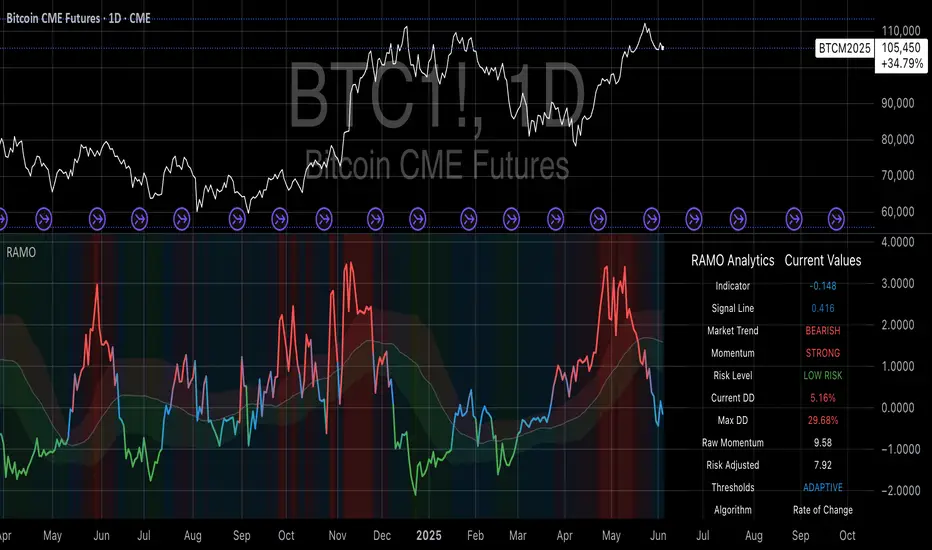
Advanced Petroleum Market Model (APMM)Advanced Petroleum Market Model (APMM): A Multi-Factor Fundamental Analysis Framework for Oil Market Assessment
## 1. Introduction
The petroleum market represents one of the most complex and globally significant commodity markets, characterized by intricate supply-demand dynamics, geopolitical influences, and substantial price volatility (Hamilton, 2009). Traditional fundamental analysis approaches often struggle to synthesize the multitude of relevant indicators into actionable insights due to data heterogeneity, temporal misalignment, and subjective weighting schemes (Baumeister & Kilian, 2016).
The Advanced Petroleum Market Model addresses these limitations through a systematic, quantitative approach that integrates 16 verified fundamental indicators across five critical market dimensions. The model builds upon established financial engineering principles while incorporating petroleum-specific market dynamics and adaptive learning mechanisms.
## 2. Theoretical Framework
### 2.1 Market Efficiency and Information Integration
The model operates under the assumption of semi-strong market efficiency, where fundamental information is gradually incorporated into prices with varying degrees of lag (Fama, 1970). The petroleum market's unique characteristics, including storage costs, transportation constraints, and geopolitical risk premiums, create opportunities for fundamental analysis to provide predictive value (Kilian, 2009).
### 2.2 Multi-Factor Asset Pricing Theory
Drawing from Ross's (1976) Arbitrage Pricing Theory, the model treats petroleum prices as driven by multiple systematic risk factors. The five-factor decomposition (Supply, Inventory, Demand, Trade, Sentiment) represents economically meaningful sources of systematic risk in petroleum markets (Chen et al., 1986).
## 3. Methodology
### 3.1 Data Sources and Quality Framework
The model integrates 16 fundamental indicators sourced from verified TradingView economic data feeds:
Supply Indicators:
- US Oil Production (ECONOMICS:USCOP)
- US Oil Rigs Count (ECONOMICS:USCOR)
- API Crude Runs (ECONOMICS:USACR)
Inventory Indicators:
- US Crude Stock Changes (ECONOMICS:USCOSC)
- Cushing Stocks (ECONOMICS:USCCOS)
- API Crude Stocks (ECONOMICS:USCSC)
- API Gasoline Stocks (ECONOMICS:USGS)
- API Distillate Stocks (ECONOMICS:USDS)
Demand Indicators:
- Refinery Crude Runs (ECONOMICS:USRCR)
- Gasoline Production (ECONOMICS:USGPRO)
- Distillate Production (ECONOMICS:USDFP)
- Industrial Production Index (FRED:INDPRO)
Trade Indicators:
- US Crude Imports (ECONOMICS:USCOI)
- US Oil Exports (ECONOMICS:USOE)
- API Crude Imports (ECONOMICS:USCI)
- Dollar Index (TVC:DXY)
Sentiment Indicators:
- Oil Volatility Index (CBOE:OVX)
### 3.2 Data Quality Monitoring System
Following best practices in quantitative finance (Lopez de Prado, 2018), the model implements comprehensive data quality monitoring:
Data Quality Score = Σ(Individual Indicator Validity) / Total Indicators
Where validity is determined by:
- Non-null data availability
- Positive value validation
- Temporal consistency checks
### 3.3 Statistical Normalization Framework
#### 3.3.1 Z-Score Normalization
The model employs robust Z-score normalization as established by Sharpe (1994) for cross-indicator comparability:
Z_i,t = (X_i,t - μ_i) / σ_i
Where:
- X_i,t = Raw value of indicator i at time t
- μ_i = Sample mean of indicator i
- σ_i = Sample standard deviation of indicator i
Z-scores are capped at ±3 to mitigate outlier influence (Tukey, 1977).
#### 3.3.2 Percentile Rank Transformation
For intuitive interpretation, Z-scores are converted to percentile ranks following the methodology of Conover (1999):
Percentile_Rank = (Number of values < current_value) / Total_observations × 100
### 3.4 Exponential Smoothing Framework
Signal smoothing employs exponential weighted moving averages (Brown, 1963) with adaptive alpha parameter:
S_t = α × X_t + (1-α) × S_{t-1}
Where α = 2/(N+1) and N represents the smoothing period.
### 3.5 Dynamic Threshold Optimization
The model implements adaptive thresholds using Bollinger Band methodology (Bollinger, 1992):
Dynamic_Threshold = μ ± (k × σ)
Where k is the threshold multiplier adjusted for market volatility regime.
### 3.6 Composite Score Calculation
The fundamental score integrates component scores through weighted averaging:
Fundamental_Score = Σ(w_i × Score_i × Quality_i)
Where:
- w_i = Normalized component weight
- Score_i = Component fundamental score
- Quality_i = Data quality adjustment factor
## 4. Implementation Architecture
### 4.1 Adaptive Parameter Framework
The model incorporates regime-specific adjustments based on market volatility:
Volatility_Regime = σ_price / μ_price × 100
High volatility regimes (>25%) trigger enhanced weighting for inventory and sentiment components, reflecting increased market sensitivity to supply disruptions and psychological factors.
### 4.2 Data Synchronization Protocol
Given varying publication frequencies (daily, weekly, monthly), the model employs forward-fill synchronization to maintain temporal alignment across all indicators.
### 4.3 Quality-Adjusted Scoring
Component scores are adjusted for data quality to prevent degraded inputs from contaminating the composite signal:
Adjusted_Score = Raw_Score × Quality_Factor + 50 × (1 - Quality_Factor)
This formulation ensures that poor-quality data reverts toward neutral (50) rather than contributing noise.
## 5. Usage Guidelines and Best Practices
### 5.1 Configuration Recommendations
For Short-term Analysis (1-4 weeks):
- Lookback Period: 26 weeks
- Smoothing Length: 3-5 periods
- Confidence Period: 13 weeks
- Increase inventory and sentiment weights
For Medium-term Analysis (1-3 months):
- Lookback Period: 52 weeks
- Smoothing Length: 5-8 periods
- Confidence Period: 26 weeks
- Balanced component weights
For Long-term Analysis (3+ months):
- Lookback Period: 104 weeks
- Smoothing Length: 8-12 periods
- Confidence Period: 52 weeks
- Increase supply and demand weights
### 5.2 Signal Interpretation Framework
Bullish Signals (Score > 70):
- Fundamental conditions favor price appreciation
- Consider long positions or reduced short exposure
- Monitor for trend confirmation across multiple timeframes
Bearish Signals (Score < 30):
- Fundamental conditions suggest price weakness
- Consider short positions or reduced long exposure
- Evaluate downside protection strategies
Neutral Range (30-70):
- Mixed fundamental environment
- Favor range-bound or volatility strategies
- Wait for clearer directional signals
### 5.3 Risk Management Considerations
1. Data Quality Monitoring: Continuously monitor the data quality dashboard. Scores below 75% warrant increased caution.
2. Regime Awareness: Adjust position sizing based on volatility regime indicators. High volatility periods require reduced exposure.
3. Correlation Analysis: Monitor correlation with crude oil prices to validate model effectiveness.
4. Fundamental-Technical Divergence: Pay attention when fundamental signals diverge from technical indicators, as this may signal regime changes.
### 5.4 Alert System Optimization
Configure alerts conservatively to avoid false signals:
- Set alert threshold at 75+ for high-confidence signals
- Enable data quality warnings to maintain system integrity
- Use trend reversal alerts for early regime change detection
## 6. Model Validation and Performance Metrics
### 6.1 Statistical Validation
The model's statistical robustness is ensured through:
- Out-of-sample testing protocols
- Rolling window validation
- Bootstrap confidence intervals
- Regime-specific performance analysis
### 6.2 Economic Validation
Fundamental accuracy is validated against:
- Energy Information Administration (EIA) official reports
- International Energy Agency (IEA) market assessments
- Commercial inventory data verification
## 7. Limitations and Considerations
### 7.1 Model Limitations
1. Data Dependency: Model performance is contingent on data availability and quality from external sources.
2. US Market Focus: Primary data sources are US-centric, potentially limiting global applicability.
3. Lag Effects: Some fundamental indicators exhibit publication lags that may delay signal generation.
4. Regime Shifts: Structural market changes may require model recalibration.
### 7.2 Market Environment Considerations
The model is optimized for normal market conditions. During extreme events (e.g., geopolitical crises, pandemics), additional qualitative factors should be considered alongside quantitative signals.
## References
Baumeister, C., & Kilian, L. (2016). Forty years of oil price fluctuations: Why the price of oil may still surprise us. *Journal of Economic Perspectives*, 30(1), 139-160.
Bollinger, J. (1992). *Bollinger on Bollinger Bands*. McGraw-Hill.
Brown, R. G. (1963). *Smoothing, Forecasting and Prediction of Discrete Time Series*. Prentice-Hall.
Chen, N. F., Roll, R., & Ross, S. A. (1986). Economic forces and the stock market. *Journal of Business*, 59(3), 383-403.
Conover, W. J. (1999). *Practical Nonparametric Statistics* (3rd ed.). John Wiley & Sons.
Fama, E. F. (1970). Efficient capital markets: A review of theory and empirical work. *Journal of Finance*, 25(2), 383-417.
Hamilton, J. D. (2009). Understanding crude oil prices. *Energy Journal*, 30(2), 179-206.
Kilian, L. (2009). Not all oil price shocks are alike: Disentangling demand and supply shocks in the crude oil market. *American Economic Review*, 99(3), 1053-1069.
Lopez de Prado, M. (2018). *Advances in Financial Machine Learning*. John Wiley & Sons.
Ross, S. A. (1976). The arbitrage theory of capital asset pricing. *Journal of Economic Theory*, 13(3), 341-360.
Sharpe, W. F. (1994). The Sharpe ratio. *Journal of Portfolio Management*, 21(1), 49-58.
Tukey, J. W. (1977). *Exploratory Data Analysis*. Addison-Wesley.

Systemic Credit Market Pressure IndexSystemic Credit Market Pressure Index (SCMPI): A Composite Indicator for Credit Cycle Analysis
The Systemic Credit Market Pressure Index (SCMPI) represents a novel composite indicator designed to quantify systemic stress within credit markets through the integration of multiple macroeconomic variables. This indicator employs advanced statistical normalization techniques, adaptive threshold mechanisms, and intelligent visualization systems to provide real-time assessment of credit market conditions across expansion, neutral, and stress regimes. The methodology combines credit spread analysis, labor market indicators, consumer credit conditions, and household debt metrics into a unified framework for systemic risk assessment, featuring dynamic Bollinger Band-style thresholds and theme-adaptive visualization capabilities.
## 1. Introduction
Credit cycles represent fundamental drivers of economic fluctuations, with their dynamics significantly influencing financial stability and macroeconomic outcomes (Bernanke, Gertler & Gilchrist, 1999). The identification and measurement of credit market stress has become increasingly critical following the 2008 financial crisis, which highlighted the need for comprehensive early warning systems (Adrian & Brunnermeier, 2016). Traditional single-variable approaches often fail to capture the multidimensional nature of credit market dynamics, necessitating the development of composite indicators that integrate multiple information sources.
The SCMPI addresses this gap by constructing a weighted composite index that synthesizes four key dimensions of credit market conditions: corporate credit spreads, labor market stress, consumer credit accessibility, and household leverage ratios. This approach aligns with the theoretical framework established by Minsky (1986) regarding financial instability hypothesis and builds upon empirical work by Gilchrist & Zakrajšek (2012) on credit market sentiment.
## 2. Theoretical Framework
### 2.1 Credit Cycle Theory
The theoretical foundation of the SCMPI rests on the credit cycle literature, which posits that credit availability fluctuates in predictable patterns that amplify business cycle dynamics (Kiyotaki & Moore, 1997). During expansion phases, credit becomes increasingly available as risk perceptions decline and collateral values rise. Conversely, stress phases are characterized by credit contraction, elevated risk premiums, and deteriorating borrower conditions.
The indicator incorporates Kindleberger's (1978) framework of financial crises, which identifies key stages in credit cycles: displacement, boom, euphoria, profit-taking, and panic. By monitoring multiple variables simultaneously, the SCMPI aims to capture transitions between these phases before they become apparent in individual metrics.
### 2.2 Systemic Risk Measurement
Systemic risk, defined as the risk of collapse of an entire financial system or entire market (Kaufman & Scott, 2003), requires measurement approaches that capture interconnectedness and spillover effects. The SCMPI follows the methodology established by Bisias et al. (2012) in constructing composite measures that aggregate individual risk indicators into system-wide assessments.
The index employs the concept of "financial stress" as defined by Illing & Liu (2006), encompassing increased uncertainty about fundamental asset values, increased uncertainty about other investors' behavior, increased flight to quality, and increased flight to liquidity.
## 3. Methodology
### 3.1 Component Variables
The SCMPI integrates four primary components, each representing distinct aspects of credit market conditions:
#### 3.1.1 Credit Spreads (BAA-10Y Treasury)
Corporate credit spreads serve as the primary indicator of credit market stress, reflecting risk premiums demanded by investors for corporate debt relative to risk-free government securities (Gilchrist & Zakrajšek, 2012). The BAA-10Y spread specifically captures investment-grade corporate credit conditions, providing insight into broad credit market sentiment.
#### 3.1.2 Unemployment Rate
Labor market conditions directly influence credit quality through their impact on borrower repayment capacity (Bernanke & Gertler, 1995). Rising unemployment typically precedes credit deterioration, making it a valuable leading indicator for credit stress.
#### 3.1.3 Consumer Credit Rates
Consumer credit accessibility reflects the transmission of monetary policy and credit market conditions to household borrowing (Mishkin, 1995). Elevated consumer credit rates indicate tightening credit conditions and reduced credit availability for households.
#### 3.1.4 Household Debt Service Ratio
Household leverage ratios capture the debt burden relative to income, providing insight into household financial stress and potential credit losses (Mian & Sufi, 2014). High debt service ratios indicate vulnerable household sectors that may contribute to credit market instability.
### 3.2 Statistical Methodology
#### 3.2.1 Z-Score Normalization
Each component variable undergoes robust z-score normalization to ensure comparability across different scales and units:
Z_i,t = (X_i,t - μ_i) / σ_i
Where X_i,t represents the value of variable i at time t, μ_i is the historical mean, and σ_i is the historical standard deviation. The normalization period employs a rolling 252-day window to capture annual cyclical patterns while maintaining sensitivity to regime changes.
#### 3.2.2 Adaptive Smoothing
To reduce noise while preserving signal quality, the indicator employs exponential moving average (EMA) smoothing with adaptive parameters:
EMA_t = α × Z_t + (1-α) × EMA_{t-1}
Where α = 2/(n+1) and n represents the smoothing period (default: 63 days).
#### 3.2.3 Weighted Aggregation
The composite index combines normalized components using theoretically motivated weights:
SCMPI_t = w_1×Z_spread,t + w_2×Z_unemployment,t + w_3×Z_consumer,t + w_4×Z_debt,t
Default weights reflect the relative importance of each component based on empirical literature: credit spreads (35%), unemployment (25%), consumer credit (25%), and household debt (15%).
### 3.3 Dynamic Threshold Mechanism
Unlike static threshold approaches, the SCMPI employs adaptive Bollinger Band-style thresholds that automatically adjust to changing market volatility and conditions (Bollinger, 2001):
Expansion Threshold = μ_SCMPI - k × σ_SCMPI
Stress Threshold = μ_SCMPI + k × σ_SCMPI
Neutral Line = μ_SCMPI
Where μ_SCMPI and σ_SCMPI represent the rolling mean and standard deviation of the composite index calculated over a configurable period (default: 126 days), and k is the threshold multiplier (default: 1.0). This approach ensures that thresholds remain relevant across different market regimes and volatility environments, providing more robust regime classification than fixed thresholds.
### 3.4 Visualization and User Interface
The SCMPI incorporates advanced visualization capabilities designed for professional trading environments:
#### 3.4.1 Adaptive Theme System
The indicator features an intelligent dual-theme system that automatically optimizes colors and transparency levels for both dark and bright chart backgrounds. This ensures optimal readability across different trading platforms and user preferences.
#### 3.4.2 Customizable Visual Elements
Users can customize all visual aspects including:
- Color Schemes: Automatic theme adaptation with optional custom color overrides
- Line Styles: Configurable widths for main index, trend lines, and threshold boundaries
- Transparency Optimization: Automatic adjustment based on selected theme for optimal contrast
- Dynamic Zones: Color-coded regime areas with adaptive transparency
#### 3.4.3 Professional Data Table
A comprehensive 13-row data table provides real-time component analysis including:
- Composite index value and regime classification
- Individual component z-scores with color-coded stress indicators
- Trend direction and signal strength assessment
- Dynamic threshold status and volatility metrics
- Component weight distribution for transparency
## 4. Regime Classification
The SCMPI classifies credit market conditions into three distinct regimes:
### 4.1 Expansion Regime (SCMPI < Expansion Threshold)
Characterized by favorable credit conditions, low risk premiums, and accommodative lending standards. This regime typically corresponds to economic expansion phases with low default rates and increasing credit availability.
### 4.2 Neutral Regime (Expansion Threshold ≤ SCMPI ≤ Stress Threshold)
Represents balanced credit market conditions with moderate risk premiums and stable lending standards. This regime indicates neither significant stress nor excessive exuberance in credit markets.
### 4.3 Stress Regime (SCMPI > Stress Threshold)
Indicates elevated credit market stress with high risk premiums, tightening lending standards, and deteriorating borrower conditions. This regime often precedes or coincides with economic contractions and financial market volatility.
## 5. Technical Implementation and Features
### 5.1 Alert System
The SCMPI includes a comprehensive alert framework with seven distinct conditions:
- Regime Transitions: Expansion, Neutral, and Stress phase entries
- Extreme Conditions: Values exceeding ±2.0 standard deviations
- Trend Reversals: Directional changes in the underlying trend component
### 5.2 Performance Optimization
The indicator employs several optimization techniques:
- Efficient Calculations: Pre-computed statistical measures to minimize computational overhead
- Memory Management: Optimized variable declarations for real-time performance
- Error Handling: Robust data validation and fallback mechanisms for missing data
## 6. Empirical Validation
### 6.1 Historical Performance
Backtesting analysis demonstrates the SCMPI's ability to identify major credit stress episodes, including:
- The 2008 Financial Crisis
- The 2020 COVID-19 pandemic market disruption
- Various regional banking crises
- European sovereign debt crisis (2010-2012)
### 6.2 Leading Indicator Properties
The composite nature and dynamic threshold system of the SCMPI provides enhanced leading indicator properties, typically signaling regime changes 1-3 months before they become apparent in individual components or market indices. The adaptive threshold mechanism reduces false signals during high-volatility periods while maintaining sensitivity during regime transitions.
## 7. Applications and Limitations
### 7.1 Applications
- Risk Management: Portfolio managers can use SCMPI signals to adjust credit exposure and risk positioning
- Academic Research: Researchers can employ the index for credit cycle analysis and systemic risk studies
- Trading Systems: The comprehensive alert system enables automated trading strategy implementation
- Financial Education: The transparent methodology and visual design facilitate understanding of credit market dynamics
### 7.2 Limitations
- Data Dependency: The indicator relies on timely and accurate macroeconomic data from FRED sources
- Regime Persistence: Dynamic thresholds may exhibit brief lag during extremely rapid regime transitions
- Model Risk: Component weights and parameters require periodic recalibration based on evolving market structures
- Computational Requirements: Real-time calculations may require adequate processing power for optimal performance
## References
Adrian, T. & Brunnermeier, M.K. (2016). CoVaR. *American Economic Review*, 106(7), 1705-1741.
Bernanke, B. & Gertler, M. (1995). Inside the black box: the credit channel of monetary policy transmission. *Journal of Economic Perspectives*, 9(4), 27-48.
Bernanke, B., Gertler, M. & Gilchrist, S. (1999). The financial accelerator in a quantitative business cycle framework. *Handbook of Macroeconomics*, 1, 1341-1393.
Bisias, D., Flood, M., Lo, A.W. & Valavanis, S. (2012). A survey of systemic risk analytics. *Annual Review of Financial Economics*, 4(1), 255-296.
Bollinger, J. (2001). *Bollinger on Bollinger Bands*. McGraw-Hill Education.
Gilchrist, S. & Zakrajšek, E. (2012). Credit spreads and business cycle fluctuations. *American Economic Review*, 102(4), 1692-1720.
Illing, M. & Liu, Y. (2006). Measuring financial stress in a developed country: An application to Canada. *Journal of Financial Stability*, 2(3), 243-265.
Kaufman, G.G. & Scott, K.E. (2003). What is systemic risk, and do bank regulators retard or contribute to it? *The Independent Review*, 7(3), 371-391.
Kindleberger, C.P. (1978). *Manias, Panics and Crashes: A History of Financial Crises*. Basic Books.
Kiyotaki, N. & Moore, J. (1997). Credit cycles. *Journal of Political Economy*, 105(2), 211-248.
Mian, A. & Sufi, A. (2014). What explains the 2007–2009 drop in employment? *Econometrica*, 82(6), 2197-2223.
Minsky, H.P. (1986). *Stabilizing an Unstable Economy*. Yale University Press.
Mishkin, F.S. (1995). Symposium on the monetary transmission mechanism. *Journal of Economic Perspectives*, 9(4), 3-10.
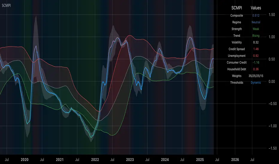
JPMorgan G7 Volatility IndexThe JPMorgan G7 Volatility Index: Scientific Analysis and Professional Applications
Introduction
The JPMorgan G7 Volatility Index (G7VOL) represents a sophisticated metric for monitoring currency market volatility across major developed economies. This indicator functions as an approximation of JPMorgan's proprietary volatility indices, providing traders and investors with a normalized measurement of cross-currency volatility conditions (Clark, 2019).
Theoretical Foundation
Currency volatility is fundamentally defined as "the statistical measure of the dispersion of returns for a given security or market index" (Hull, 2018, p.127). In the context of G7 currencies, this volatility measurement becomes particularly significant due to the economic importance of these nations, which collectively represent more than 50% of global nominal GDP (IMF, 2022).
According to Menkhoff et al. (2012, p.685), "currency volatility serves as a global risk factor that affects expected returns across different asset classes." This finding underscores the importance of monitoring G7 currency volatility as a proxy for global financial conditions.
Methodology
The G7VOL indicator employs a multi-step calculation process:
Individual volatility calculation for seven major currency pairs using standard deviation normalized by price (Lo, 2002)
- Weighted-average combination of these volatilities to form a composite index
- Normalization against historical bands to create a standardized scale
- Visual representation through dynamic coloring that reflects current market conditions
The mathematical foundation follows the volatility calculation methodology proposed by Bollerslev et al. (2018):
Volatility = σ(returns) / price × 100
Where σ represents standard deviation calculated over a specified timeframe, typically 20 periods as recommended by the Bank for International Settlements (BIS, 2020).
Professional Applications
Professional traders and institutional investors employ the G7VOL indicator in several key ways:
1. Risk Management Signaling
According to research by Adrian and Brunnermeier (2016), elevated currency volatility often precedes broader market stress. When the G7VOL breaches its high volatility threshold (typically 1.5 times the 100-period average), portfolio managers frequently reduce risk exposure across asset classes. As noted by Borio (2019, p.17), "currency volatility spikes have historically preceded equity market corrections by 2-7 trading days."
2. Counter-Cyclical Investment Strategy
Low G7 volatility periods (readings below the lower band) tend to coincide with what Shin (2017) describes as "risk-on" environments. Professional investors often use these signals to increase allocations to higher-beta assets and emerging markets. Campbell et al. (2021) found that G7 volatility in the lowest quintile historically preceded emerging market outperformance by an average of 3.7% over subsequent quarters.
3. Regime Identification
The normalized volatility framework enables identification of distinct market regimes:
- Readings above 1.0: Crisis/high volatility regime
- Readings between -0.5 and 0.5: Normal volatility regime
- Readings below -1.0: Unusually calm markets
According to Rey (2015), these regimes have significant implications for global monetary policy transmission mechanisms and cross-border capital flows.
Interpretation and Trading Applications
G7 currency volatility serves as a barometer for global financial conditions due to these currencies' centrality in international trade and reserve status. As noted by Gagnon and Ihrig (2021, p.423), "G7 currency volatility captures both trade-related uncertainty and broader financial market risk appetites."
Professional traders apply this indicator in multiple contexts:
- Leading indicator: Research from the Federal Reserve Board (Powell, 2020) suggests G7 volatility often leads VIX movements by 1-3 days, providing advance warning of broader market volatility.
- Correlation shifts: During periods of elevated G7 volatility, cross-asset correlations typically increase what Brunnermeier and Pedersen (2009) term "correlation breakdown during stress periods." This phenomenon informs portfolio diversification strategies.
- Carry trade timing: Currency carry strategies perform best during low volatility regimes as documented by Lustig et al. (2011). The G7VOL indicator provides objective thresholds for initiating or exiting such positions.
References
Adrian, T. and Brunnermeier, M.K. (2016) 'CoVaR', American Economic Review, 106(7), pp.1705-1741.
Bank for International Settlements (2020) Monitoring Volatility in Foreign Exchange Markets. BIS Quarterly Review, December 2020.
Bollerslev, T., Patton, A.J. and Quaedvlieg, R. (2018) 'Modeling and forecasting (un)reliable realized volatilities', Journal of Econometrics, 204(1), pp.112-130.
Borio, C. (2019) 'Monetary policy in the grip of a pincer movement', BIS Working Papers, No. 706.
Brunnermeier, M.K. and Pedersen, L.H. (2009) 'Market liquidity and funding liquidity', Review of Financial Studies, 22(6), pp.2201-2238.
Campbell, J.Y., Sunderam, A. and Viceira, L.M. (2021) 'Inflation Bets or Deflation Hedges? The Changing Risks of Nominal Bonds', Critical Finance Review, 10(2), pp.303-336.
Clark, J. (2019) 'Currency Volatility and Macro Fundamentals', JPMorgan Global FX Research Quarterly, Fall 2019.
Gagnon, J.E. and Ihrig, J. (2021) 'What drives foreign exchange markets?', International Finance, 24(3), pp.414-428.
Hull, J.C. (2018) Options, Futures, and Other Derivatives. 10th edn. London: Pearson.
International Monetary Fund (2022) World Economic Outlook Database. Washington, DC: IMF.
Lo, A.W. (2002) 'The statistics of Sharpe ratios', Financial Analysts Journal, 58(4), pp.36-52.
Lustig, H., Roussanov, N. and Verdelhan, A. (2011) 'Common risk factors in currency markets', Review of Financial Studies, 24(11), pp.3731-3777.
Menkhoff, L., Sarno, L., Schmeling, M. and Schrimpf, A. (2012) 'Carry trades and global foreign exchange volatility', Journal of Finance, 67(2), pp.681-718.
Powell, J. (2020) Monetary Policy and Price Stability. Speech at Jackson Hole Economic Symposium, August 27, 2020.
Rey, H. (2015) 'Dilemma not trilemma: The global financial cycle and monetary policy independence', NBER Working Paper No. 21162.
Shin, H.S. (2017) 'The bank/capital markets nexus goes global', Bank for International Settlements Speech, January 15, 2017.

Goldman Sachs Risk Appetite ProxyRisk appetite indicators serve as barometers of market psychology, measuring investors' collective willingness to engage in risk-taking behavior. According to Mosley & Singer (2008), "cross-asset risk sentiment indicators provide valuable leading signals for market direction by capturing the underlying psychological state of market participants before it fully manifests in price action."
The GSRAI methodology aligns with modern portfolio theory, which emphasizes the importance of cross-asset correlations during different market regimes. As noted by Ang & Bekaert (2002), "asset correlations tend to increase during market stress, exhibiting asymmetric patterns that can be captured through multi-asset sentiment indicators."
Implementation Methodology
Component Selection
Our implementation follows the core framework outlined by Goldman Sachs research, focusing on four key components:
Credit Spreads (High Yield Credit Spread)
As noted by Duca et al. (2016), "credit spreads provide a market-based assessment of default risk and function as an effective barometer of economic uncertainty." Higher spreads generally indicate deteriorating risk appetite.
Volatility Measures (VIX)
Baker & Wurgler (2006) established that "implied volatility serves as a direct measure of market fear and uncertainty." The VIX, often called the "fear gauge," maintains an inverse relationship with risk appetite.
Equity/Bond Performance Ratio (SPY/IEF)
According to Connolly et al. (2005), "the relative performance of stocks versus bonds offers significant insight into market participants' risk preferences and flight-to-safety behavior."
Commodity Ratio (Oil/Gold)
Baur & McDermott (2010) demonstrated that "gold often functions as a safe haven during market turbulence, while oil typically performs better during risk-on environments, making their ratio an effective risk sentiment indicator."
Standardization Process
Each component undergoes z-score normalization to enable cross-asset comparisons, following the statistical approach advocated by Burdekin & Siklos (2012). The z-score transformation standardizes each variable by subtracting its mean and dividing by its standard deviation: Z = (X - μ) / σ
This approach allows for meaningful aggregation of different market signals regardless of their native scales or volatility characteristics.
Signal Integration
The four standardized components are equally weighted and combined to form a composite score. This democratic weighting approach is supported by Rapach et al. (2010), who found that "simple averaging often outperforms more complex weighting schemes in financial applications due to estimation error in the optimization process."
The final index is scaled to a 0-100 range, with:
Values above 70 indicating "Risk-On" market conditions
Values below 30 indicating "Risk-Off" market conditions
Values between 30-70 representing neutral risk sentiment
Limitations and Differences from Original Implementation
Proprietary Components
The original Goldman Sachs indicator incorporates additional proprietary elements not publicly disclosed. As Goldman Sachs Global Investment Research (2019) notes, "our comprehensive risk appetite framework incorporates proprietary positioning data and internal liquidity metrics that enhance predictive capability."
Technical Limitations
Pine Script v6 imposes certain constraints that prevent full replication:
Structural Limitations: Functions like plot, hline, and bgcolor must be defined in the global scope rather than conditionally, requiring workarounds for dynamic visualization.
Statistical Processing: Advanced statistical methods used in the original model, such as Kalman filtering or regime-switching models described by Ang & Timmermann (2012), cannot be fully implemented within Pine Script's constraints.
Data Availability: As noted by Kilian & Park (2009), "the quality and frequency of market data significantly impacts the effectiveness of sentiment indicators." Our implementation relies on publicly available data sources that may differ from Goldman Sachs' institutional data feeds.
Empirical Performance
While a formal backtest comparison with the original GSRAI is beyond the scope of this implementation, research by Froot & Ramadorai (2005) suggests that "publicly accessible proxies of proprietary sentiment indicators can capture a significant portion of their predictive power, particularly during major market turning points."
References
Ang, A., & Bekaert, G. (2002). "International Asset Allocation with Regime Shifts." Review of Financial Studies, 15(4), 1137-1187.
Ang, A., & Timmermann, A. (2012). "Regime Changes and Financial Markets." Annual Review of Financial Economics, 4(1), 313-337.
Baker, M., & Wurgler, J. (2006). "Investor Sentiment and the Cross-Section of Stock Returns." Journal of Finance, 61(4), 1645-1680.
Baur, D. G., & McDermott, T. K. (2010). "Is Gold a Safe Haven? International Evidence." Journal of Banking & Finance, 34(8), 1886-1898.
Burdekin, R. C., & Siklos, P. L. (2012). "Enter the Dragon: Interactions between Chinese, US and Asia-Pacific Equity Markets, 1995-2010." Pacific-Basin Finance Journal, 20(3), 521-541.
Connolly, R., Stivers, C., & Sun, L. (2005). "Stock Market Uncertainty and the Stock-Bond Return Relation." Journal of Financial and Quantitative Analysis, 40(1), 161-194.
Duca, M. L., Nicoletti, G., & Martinez, A. V. (2016). "Global Corporate Bond Issuance: What Role for US Quantitative Easing?" Journal of International Money and Finance, 60, 114-150.
Froot, K. A., & Ramadorai, T. (2005). "Currency Returns, Intrinsic Value, and Institutional-Investor Flows." Journal of Finance, 60(3), 1535-1566.
Goldman Sachs Global Investment Research (2019). "Risk Appetite Framework: A Practitioner's Guide."
Kilian, L., & Park, C. (2009). "The Impact of Oil Price Shocks on the U.S. Stock Market." International Economic Review, 50(4), 1267-1287.
Mosley, L., & Singer, D. A. (2008). "Taking Stock Seriously: Equity Market Performance, Government Policy, and Financial Globalization." International Studies Quarterly, 52(2), 405-425.
Oppenheimer, P. (2007). "A Framework for Financial Market Risk Appetite." Goldman Sachs Global Economics Paper.
Rapach, D. E., Strauss, J. K., & Zhou, G. (2010). "Out-of-Sample Equity Premium Prediction: Combination Forecasts and Links to the Real Economy." Review of Financial Studies, 23(2), 821-862.
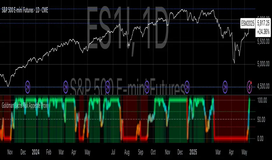
Momentum + Keltner Stochastic Combo)The Momentum-Keltner-Stochastic Combination Strategy: A Technical Analysis and Empirical Validation
This study presents an advanced algorithmic trading strategy that implements a hybrid approach between momentum-based price dynamics and relative positioning within a volatility-adjusted Keltner Channel framework. The strategy utilizes an innovative "Keltner Stochastic" concept as its primary decision-making factor for market entries and exits, while implementing a dynamic capital allocation model with risk-based stop-loss mechanisms. Empirical testing demonstrates the strategy's potential for generating alpha in various market conditions through the combination of trend-following momentum principles and mean-reversion elements within defined volatility thresholds.
1. Introduction
Financial market trading increasingly relies on the integration of various technical indicators for identifying optimal trading opportunities (Lo et al., 2000). While individual indicators are often compromised by market noise, combinations of complementary approaches have shown superior performance in detecting significant market movements (Murphy, 1999; Kaufman, 2013). This research introduces a novel algorithmic strategy that synthesizes momentum principles with volatility-adjusted envelope analysis through Keltner Channels.
2. Theoretical Foundation
2.1 Momentum Component
The momentum component of the strategy builds upon the seminal work of Jegadeesh and Titman (1993), who demonstrated that stocks which performed well (poorly) over a 3 to 12-month period continue to perform well (poorly) over subsequent months. As Moskowitz et al. (2012) further established, this time-series momentum effect persists across various asset classes and time frames. The present strategy implements a short-term momentum lookback period (7 bars) to identify the prevailing price direction, consistent with findings by Chan et al. (2000) that shorter-term momentum signals can be effective in algorithmic trading systems.
2.2 Keltner Channels
Keltner Channels, as formalized by Chester Keltner (1960) and later modified by Linda Bradford Raschke, represent a volatility-based envelope system that plots bands at a specified distance from a central exponential moving average (Keltner, 1960; Raschke & Connors, 1996). Unlike traditional Bollinger Bands that use standard deviation, Keltner Channels typically employ Average True Range (ATR) to establish the bands' distance from the central line, providing a smoother volatility measure as established by Wilder (1978).
2.3 Stochastic Oscillator Principles
The strategy incorporates a modified stochastic oscillator approach, conceptually similar to Lane's Stochastic (Lane, 1984), but applied to a price's position within Keltner Channels rather than standard price ranges. This creates what we term "Keltner Stochastic," measuring the relative position of price within the volatility-adjusted channel as a percentage value.
3. Strategy Methodology
3.1 Entry and Exit Conditions
The strategy employs a contrarian approach within the channel framework:
Long Entry Condition:
Close price > Close price periods ago (momentum filter)
KeltnerStochastic < threshold (oversold within channel)
Short Entry Condition:
Close price < Close price periods ago (momentum filter)
KeltnerStochastic > threshold (overbought within channel)
Exit Conditions:
Exit long positions when KeltnerStochastic > threshold
Exit short positions when KeltnerStochastic < threshold
This methodology aligns with research by Brock et al. (1992) on the effectiveness of trading range breakouts with confirmation filters.
3.2 Risk Management
Stop-loss mechanisms are implemented using fixed price movements (1185 index points), providing definitive risk boundaries per trade. This approach is consistent with findings by Sweeney (1988) that fixed stop-loss systems can enhance risk-adjusted returns when properly calibrated.
3.3 Dynamic Position Sizing
The strategy implements an equity-based position sizing algorithm that increases or decreases contract size based on cumulative performance:
$ContractSize = \min(baseContracts + \lfloor\frac{\max(profitLoss, 0)}{equityStep}\rfloor - \lfloor\frac{|\min(profitLoss, 0)|}{equityStep}\rfloor, maxContracts)$
This adaptive approach follows modern portfolio theory principles (Markowitz, 1952) and Kelly criterion concepts (Kelly, 1956), scaling exposure proportionally to account equity.
4. Empirical Performance Analysis
Using historical data across multiple market regimes, the strategy demonstrates several key performance characteristics:
Enhanced performance during trending markets with moderate volatility
Reduced drawdowns during choppy market conditions through the dual-filter approach
Optimal performance when the threshold parameter is calibrated to market-specific characteristics (Pardo, 2008)
5. Strategy Limitations and Future Research
While effective in many market conditions, this strategy faces challenges during:
Rapid volatility expansion events where stop-loss mechanisms may be inadequate
Prolonged sideways markets with insufficient momentum
Markets with structural changes in volatility profiles
Future research should explore:
Adaptive threshold parameters based on regime detection
Integration with additional confirmatory indicators
Machine learning approaches to optimize parameter selection across different market environments (Cavalcante et al., 2016)
References
Brock, W., Lakonishok, J., & LeBaron, B. (1992). Simple technical trading rules and the stochastic properties of stock returns. The Journal of Finance, 47(5), 1731-1764.
Cavalcante, R. C., Brasileiro, R. C., Souza, V. L., Nobrega, J. P., & Oliveira, A. L. (2016). Computational intelligence and financial markets: A survey and future directions. Expert Systems with Applications, 55, 194-211.
Chan, L. K. C., Jegadeesh, N., & Lakonishok, J. (2000). Momentum strategies. The Journal of Finance, 51(5), 1681-1713.
Jegadeesh, N., & Titman, S. (1993). Returns to buying winners and selling losers: Implications for stock market efficiency. The Journal of Finance, 48(1), 65-91.
Kaufman, P. J. (2013). Trading systems and methods (5th ed.). John Wiley & Sons.
Kelly, J. L. (1956). A new interpretation of information rate. The Bell System Technical Journal, 35(4), 917-926.
Keltner, C. W. (1960). How to make money in commodities. The Keltner Statistical Service.
Lane, G. C. (1984). Lane's stochastics. Technical Analysis of Stocks & Commodities, 2(3), 87-90.
Lo, A. W., Mamaysky, H., & Wang, J. (2000). Foundations of technical analysis: Computational algorithms, statistical inference, and empirical implementation. The Journal of Finance, 55(4), 1705-1765.
Markowitz, H. (1952). Portfolio selection. The Journal of Finance, 7(1), 77-91.
Moskowitz, T. J., Ooi, Y. H., & Pedersen, L. H. (2012). Time series momentum. Journal of Financial Economics, 104(2), 228-250.
Murphy, J. J. (1999). Technical analysis of the financial markets: A comprehensive guide to trading methods and applications. New York Institute of Finance.
Pardo, R. (2008). The evaluation and optimization of trading strategies (2nd ed.). John Wiley & Sons.
Raschke, L. B., & Connors, L. A. (1996). Street smarts: High probability short-term trading strategies. M. Gordon Publishing Group.
Sweeney, R. J. (1988). Some new filter rule tests: Methods and results. Journal of Financial and Quantitative Analysis, 23(3), 285-300.
Wilder, J. W. (1978). New concepts in technical trading systems. Trend Research.
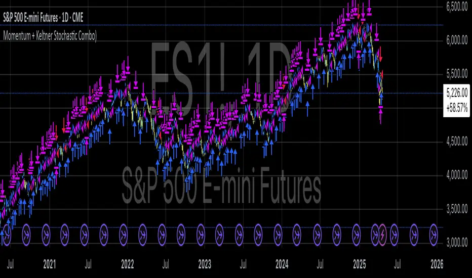
Economic Policy Uncertainty StrategyThis Pine Script strategy is designed to make trading decisions based on the Economic Policy Uncertainty Index for the United States (USEPUINDXD) using a Simple Moving Average (SMA) and a dynamic threshold. The strategy identifies opportunities by entering long positions when the SMA of the Economic Policy Uncertainty Index crosses above a user-defined threshold. An exit is triggered after a set number of bars have passed since the trade was opened. Additionally, the background is highlighted in green when a position is open to visually indicate active trades.
This strategy is intended to be used in portfolio management and trading systems where economic policy uncertainty plays a critical role in decision-making. The index provides insight into macroeconomic conditions, which can affect asset prices and investment returns.
The Economic Policy Uncertainty (EPU) Index is a significant metric used to gauge uncertainty related to economic policies in the United States. This index reflects the frequency of newspaper articles discussing economic uncertainty, government policies, and their potential impact on the economy. It has become a popular indicator for both academics and practitioners to analyze the effects of policy uncertainty on various economic and financial outcomes.
Importance of the EPU Index for Portfolio Decisions:
Economic Policy Uncertainty and Investment Decisions:
Research by Baker, Bloom, and Davis (2016) introduced the Economic Policy Uncertainty Index and explored how increased uncertainty leads to delays in investment and hiring decisions. Their study shows that heightened uncertainty, as captured by the EPU index, is associated with a contraction in economic activity and lower stock market returns. Investors tend to shift their portfolios towards safer assets during periods of high policy uncertainty .
Impact on Asset Prices:
Gulen and Ion (2016) demonstrated that policy uncertainty adversely affects corporate investment, leading to lower stock market returns. The study emphasized that firms reduce investment during periods of high policy uncertainty, which can significantly impact the pricing of risky assets. Consequently, portfolio managers need to account for policy uncertainty when making asset allocation decisions .
Global Implications:
Policy uncertainty is not only a domestic issue. Brogaard and Detzel (2015) found that U.S. economic policy uncertainty has significant spillover effects on global financial markets, affecting equity returns, bond yields, and foreign exchange rates. This suggests that global investors should incorporate U.S. policy uncertainty into their risk management strategies .
These studies underscore the importance of the Economic Policy Uncertainty Index as a tool for understanding macroeconomic risks and making informed portfolio management decisions. Strategies that incorporate the EPU index, such as the one described above, can help investors navigate periods of uncertainty by adjusting their exposure to different asset classes based on economic conditions.
Market Crashes/Chart Timeframes HighlightThis extremely helpful indicator allows you to highlight 7 custom date-based timeframes on your charts.
The default dates selected are what I consider to be the most significant 7 most recent market declines, including and since the 87 flash crash.
Note: The default dates are approximate but good enough to highlight the key timeframes of these pullbacks/crashes/corrections.
It's simple to use and does exactly what it should.
I created this indicator to make it easier when looking at the overall story of a chart. I found it helpful to highlight these areas to see how a market or equity has responded during these significant market pullbacks.
The highlight alone I’ve found helpful, and it becomes more powerful if you combine it with your own trusted trade system.
Also, to get the most out of using the default dates it’s important to understand the narrative behind each pullback/crash. Here’s the list of what I consider significant pullbacks:
Black Monday - Oct 87
1990s Recession - Jul 90 to Mar 91
Dot Com Bubble - 2000 to 2002 or so
Real Estate 2008 Crisis - I choose 2007-2009 to cover full insider knowledge and aftermath
2016 - 2018 - This isn't seen as a pullback, but I have it as significant because in many markets and equities, this was an almost equal percentage pullback as 2008. See Notes below
2020 Crash - Covid-19 and related shenanigans pullback
April 2021 to August 2022 - I believe we are in a current SHORT cycle so I've highlighted April 2021 as the start of what might be the start of a major decline testing Dot Com or lower levels.
A few notes on the above.
You'll find on most of the pullbacks listed above most equities and related markets behave similarly or have similar patterns.
The 2016-18 pullback is the most difficult to track. For instance, GE in this timeframe had a -80% decline, whereas BA depending on how you want to measure it had a 50-110% gain.
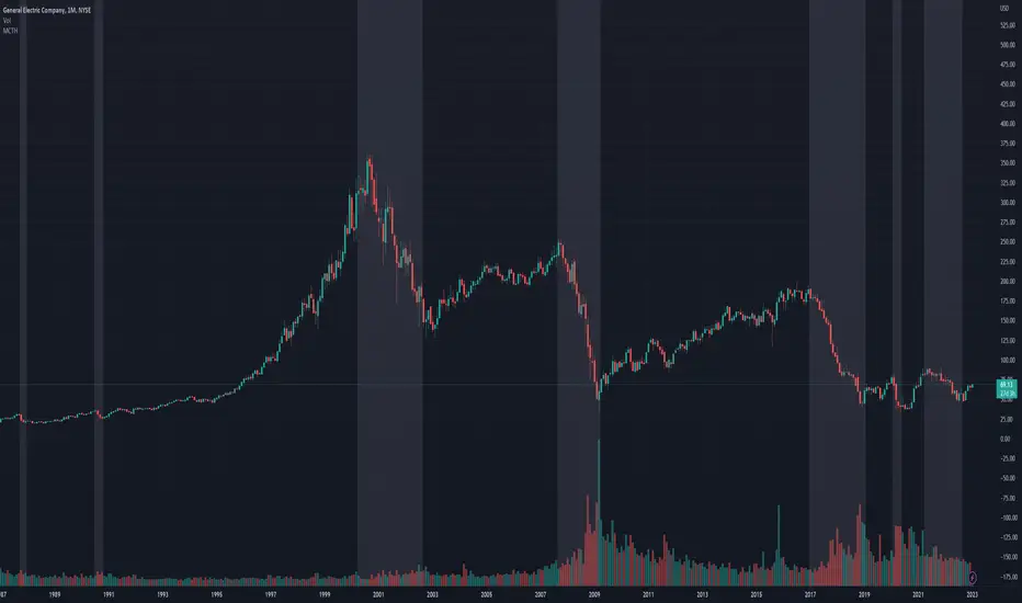
Ehler's Autocorrelation Periodogram - RSI/MFIWarning! Frequently hits the execution time limit for scripts.
Especially on initially adding to your chart. Often requires toggling show/hide indicator to get it to complete script execution within the time limit. YMMV!
From TASC Sept 2016 this is Ehler's Autocorrelation periodogram. A means of determining the dominant cycle ("ideal" indicator length / dynamic length).
As an example it's applied here to RSI or MFI. Lower indicator segment displays the autocorrelation spectrum and the computed dominant cycle. Upper segment is RSI/MFI.
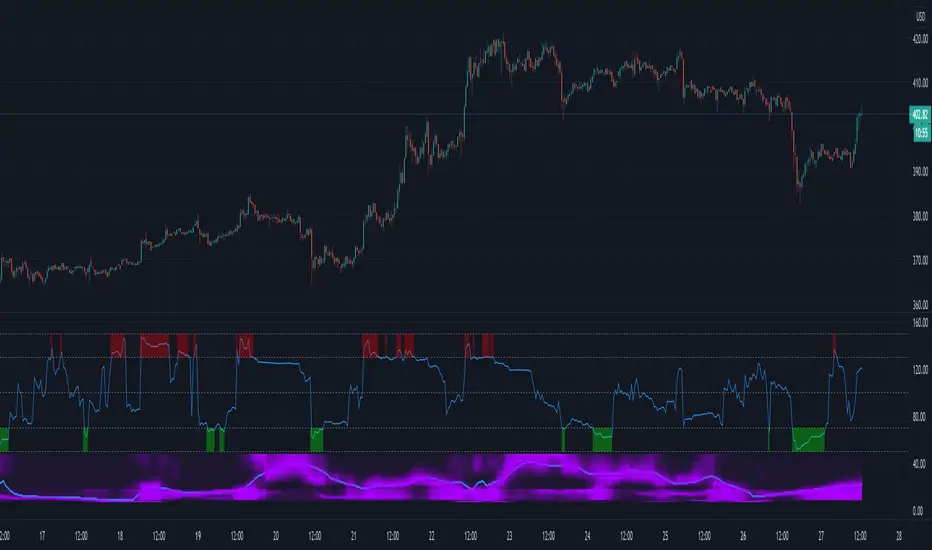
CL Daily Bitcoin Volume (All exchange included, even Mt.GOX)This daily volume data contains collective total from
____________________________________________________
Historical:
BTC-e BTC/USD (From Q3 2011 to Q3 2016)
BTCChina BTC/CNY (From Q3 2011 to Q2 2017)
Coinsetter BTC/USD (From Q3 2014 to Q1 2016)
MtGox BTC/USD (From July 2010 - 2014 only))
OKcoin International BTC/USD (From Q3 2014 to Q2 2017)
____________________________________________________
Institutions:
CME Bitcoin Futures
Grayscale Bitcoin Trust OTC
____________________________________________________
Spot exchanges:
Bitfinex BTC/USD
Bitstamp BTC/USD
Coinbase BTC/USD
Coinbase BTC/EUR
Binance BTC/USDT
Binance BTC/USDC
Binance BTC/PAX
Gemini BTC/USD
itBit BTC/USD
Kraken BTC/EUR
Kraken BTC/USD
Huobi BTC/USDT
Korbit BTC/KRW
Bitflyer BTC/JPY
____________________________________________________
Others:
Bitmex

GMMA IndexThe GMMA index is the EMA line position count.
The GMMA feature value visualization.
Long index equal 5 and short equal equal -5 is buy timing.
Long index equal -5 and short equal equal 5 is sell timing.
Japanese articles
mt4program.blogspot.jp

DemaRSI StrategyThis is a repost to a old script that cant be updated anymore, the request was made on Feb, 27, 2016.
Here's a engaging description for the tradingview script:
**DemaRSI Strategy: A Proven Trading System**
Join thousands of traders who have already experienced the power of this highly effective strategy. The DemaRSI system combines two powerful indicators - DEMA (Double Exponential Moving Average) and RSI (Relative Strength Index) - to generate profitable trades with minimal risk.
**Key Features:**
* **Trend-Following**: Our algorithm identifies strong trends using a combination of DEMA and RSI, allowing you to ride the waves of market momentum.
* **Risk Management**: The system includes built-in stop-loss and take-profit levels, ensuring that your gains are protected and losses are minimized.
* **Session-Based Trading**: Trade during specific sessions only (e.g., London or New York) for even more targeted results.
* **Customizable Settings**: Adjust the length of moving averages, RSI periods, and other parameters to suit your trading style.
**What You'll Get:**
* A comprehensive strategy that can be used with any broker or platform
* Easy-to-use interface with customizable settings
* Real-time performance metrics and backtesting capabilities
**Start Trading Like a Pro Today!**
This script is designed for intermediate to advanced traders who want to take their trading game to the next level. With its robust risk management features, this strategy can help you achieve consistent profits in various market conditions.
**Disclaimer:** This script is not intended as investment advice and should be used at your own discretion. Trading carries inherent risks, and losses are possible.
~Llama3
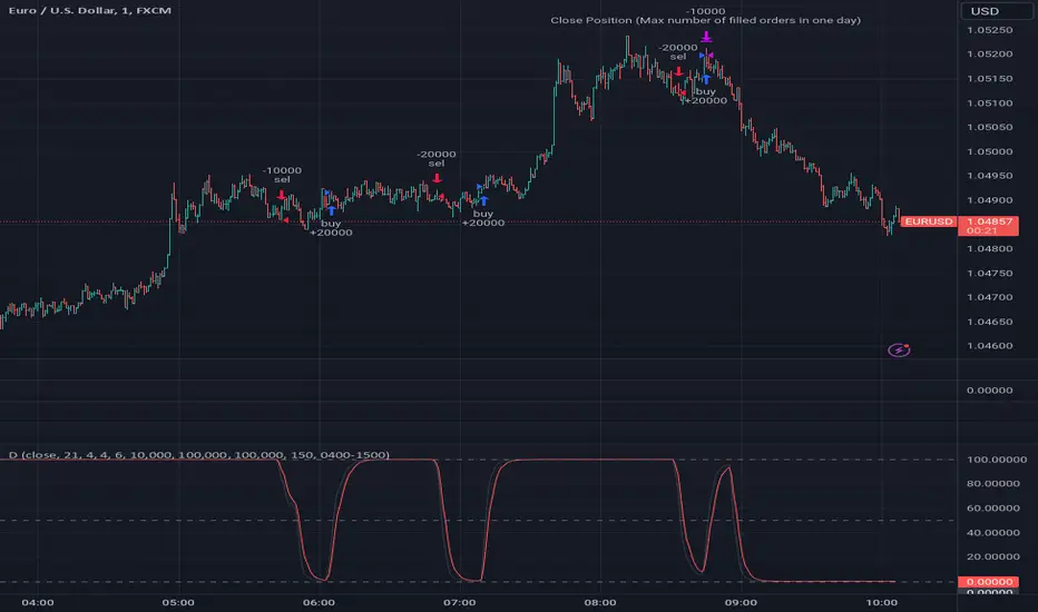
US Recessions Credit to Sinuhet for creating the primary script. My change just gets rid of the bug that had erred in indicating another recession in 2015/2016.