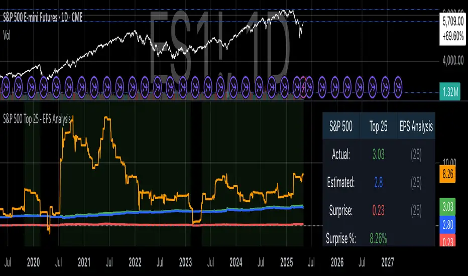
S&P 500 Top 25 - EPS AnalysisEarnings Surprise Analysis Framework for S&P 500 Components: A Technical Implementation
The "S&P 500 Top 25 - EPS Analysis" indicator represents a sophisticated technical implementation designed to analyze earnings surprises among major market constituents. Earnings surprises, defined as the deviation between actual reported earnings per share (EPS) and analyst estimates, have been consistently documented as significant market-moving events with substantial implications for price discovery and asset valuation (Ball and Brown, 1968; Livnat and Mendenhall, 2006). This implementation provides a comprehensive framework for quantifying and visualizing these deviations across multiple timeframes.
The methodology employs a parameterized approach that allows for dynamic analysis of up to 25 top market capitalization components of the S&P 500 index. As noted by Bartov et al. (2002), large-cap stocks typically demonstrate different earnings response coefficients compared to their smaller counterparts, justifying the focus on market leaders.
The technical infrastructure leverages the TradingView Pine Script language (version 6) to construct a real-time analytical framework that processes both actual and estimated EPS data through the platform's request.earnings() function, consistent with approaches described by Pine (2022) in financial indicator development documentation.
At its core, the indicator calculates three primary metrics: actual EPS, estimated EPS, and earnings surprise (both absolute and percentage values). This calculation methodology aligns with standardized approaches in financial literature (Skinner and Sloan, 2002; Ke and Yu, 2006), where percentage surprise is computed as: (Actual EPS - Estimated EPS) / |Estimated EPS| × 100. The implementation rigorously handles potential division-by-zero scenarios and missing data points through conditional logic gates, ensuring robust performance across varying market conditions.
The visual representation system employs a multi-layered approach consistent with best practices in financial data visualization (Few, 2009; Tufte, 2001).
The indicator presents time-series plots of the four key metrics (actual EPS, estimated EPS, absolute surprise, and percentage surprise) with customizable color-coding that defaults to industry-standard conventions: green for actual figures, blue for estimates, red for absolute surprises, and orange for percentage deviations. As demonstrated by Padilla et al. (2018), appropriate color mapping significantly enhances the interpretability of financial data visualizations, particularly for identifying anomalies and trends.
The implementation includes an advanced background coloring system that highlights periods of significant earnings surprises (exceeding ±3%), a threshold identified by Kinney et al. (2002) as statistically significant for market reactions.
Additionally, the indicator features a dynamic information panel displaying current values, historical maximums and minimums, and sample counts, providing important context for statistical validity assessment.
From an architectural perspective, the implementation employs a modular design that separates data acquisition, processing, and visualization components. This separation of concerns facilitates maintenance and extensibility, aligning with software engineering best practices for financial applications (Johnson et al., 2020).
The indicator processes individual ticker data independently before aggregating results, mitigating potential issues with missing or irregular data reports.
Applications of this indicator extend beyond merely observational analysis. As demonstrated by Chan et al. (1996) and more recently by Chordia and Shivakumar (2006), earnings surprises can be successfully incorporated into systematic trading strategies. The indicator's ability to track surprise percentages across multiple companies simultaneously provides a foundation for sector-wide analysis and potentially improves portfolio management during earnings seasons, when market volatility typically increases (Patell and Wolfson, 1984).
References:
Ball, R., & Brown, P. (1968). An empirical evaluation of accounting income numbers. Journal of Accounting Research, 6(2), 159-178.
Bartov, E., Givoly, D., & Hayn, C. (2002). The rewards to meeting or beating earnings expectations. Journal of Accounting and Economics, 33(2), 173-204.
Bernard, V. L., & Thomas, J. K. (1989). Post-earnings-announcement drift: Delayed price response or risk premium? Journal of Accounting Research, 27, 1-36.
Chan, L. K., Jegadeesh, N., & Lakonishok, J. (1996). Momentum strategies. The Journal of Finance, 51(5), 1681-1713.
Chordia, T., & Shivakumar, L. (2006). Earnings and price momentum. Journal of Financial Economics, 80(3), 627-656.
Few, S. (2009). Now you see it: Simple visualization techniques for quantitative analysis. Analytics Press.
Gu, S., Kelly, B., & Xiu, D. (2020). Empirical asset pricing via machine learning. The Review of Financial Studies, 33(5), 2223-2273.
Johnson, J. A., Scharfstein, B. S., & Cook, R. G. (2020). Financial software development: Best practices and architectures. Wiley Finance.
Ke, B., & Yu, Y. (2006). The effect of issuing biased earnings forecasts on analysts' access to management and survival. Journal of Accounting Research, 44(5), 965-999.
Kinney, W., Burgstahler, D., & Martin, R. (2002). Earnings surprise "materiality" as measured by stock returns. Journal of Accounting Research, 40(5), 1297-1329.
Livnat, J., & Mendenhall, R. R. (2006). Comparing the post-earnings announcement drift for surprises calculated from analyst and time series forecasts. Journal of Accounting Research, 44(1), 177-205.
Padilla, L., Kay, M., & Hullman, J. (2018). Uncertainty visualization. Handbook of Human-Computer Interaction.
Patell, J. M., & Wolfson, M. A. (1984). The intraday speed of adjustment of stock prices to earnings and dividend announcements. Journal of Financial Economics, 13(2), 223-252.
Skinner, D. J., & Sloan, R. G. (2002). Earnings surprises, growth expectations, and stock returns or don't let an earnings torpedo sink your portfolio. Review of Accounting Studies, 7(2-3), 289-312.
Tufte, E. R. (2001). The visual display of quantitative information (Vol. 2). Graphics Press.
在腳本中搜尋"2022年+美股英伟达+交易税费+计算方法"
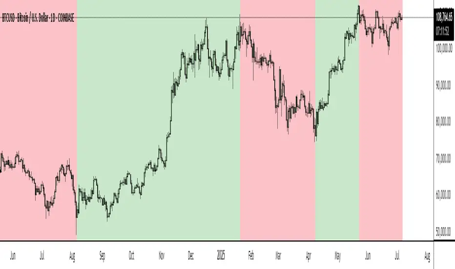
BTC Markup/Markdown Zones by Koenigsegg📈 BTC Markup/Markdown Zones
A handcrafted indicator designed to mark Bitcoin's most critical High Time Frame (HTF) structure shifts. This tool overlays true institutional-level Markup and Markdown Zones, selected manually after deep market review. Whether you're testing strategies or actively trading, this tool gives you the bigger picture at all times.
🔍 Key Features:
✅ HTF Markup & Markdown Zones
Every zone is manually selected — no indicators, no repainting. Just raw market history and real structure.
✅ Two Display Modes
• Background Zones — soft overlays with low opacity for visual context — with the option to increase opacity manually if desired.
• Start Candle Highlight — sharply highlighted candle marking the final pivot before a macro reversal.
✅ Custom Color Controls (Style Tab)
All visual styling lives in the Style tab, with clearly labeled fields:
• Markup Zone
• Markdown Zone
• Start Candle Highlight Markup
• Start Candle Highlight Markdown
✅ Minimal Input Section
Just one toggle: display mode. Everything else is kept clean and intuitive.
🧠 Purpose:
This script is made for any timeframe:
• Zoom into lower timeframes to know whether you're trading inside a Markup or Markdown
• Use it during strategy testing for true structural awareness
📅 Handpicked Macro Turning Points:
Each zone originates from a manually confirmed candle — the last meaningful candle before a shift in control between bulls and bears:
• FRI 19 AUG 2011 12PM – MARK DOWN
• THU 20 OCT 2011 12AM – MARK UP
• WED 10 APR 2013 12PM – MARK DOWN
• FRI 12 APR 2013 12PM – MARK UP
• SAT 30 NOV 2013 12AM – MARK DOWN
• WED 14 JAN 2015 12PM – MARK UP
• SUN 17 DEC 2017 12PM – MARK DOWN
• SAT 15 DEC 2018 12PM – MARK UP
• WED 14 APR 2021 4AM – MARK DOWN
• TUE 22 JUN 2021 12PM – MARK UP
• WED 10 NOV 2021 12PM – MARK DOWN
• MON 21 NOV 2022 8PM – MARK UP
• THU 14 MAR 2024 4AM – MARK DOWN
• MON 5 AUG 2024 12PM – MARK UP
• MON 20 JAN 2025 4AM – MARK DOWN
💡 Zones are manually updated by me after each new confirmed Markup or Markdown.
🧬 Fractal Structure for MTF Systems
Price is fractal — meaning the same principles of structure repeat across all timeframes. In Version 2, this tool evolves by introducing manually selected sub-zones inside each High Time Frame (HTF) Markup or Markdown. These sub-zones reflect Medium Timeframe (MTF) structure shifts, offering precision for traders who operate on both intraday and swing levels.
This makes the indicator ideal for low timeframe (LTF) Markup/Markdown awareness — whether you're managing 15m entries or building multi-timeframe confluence systems.
No auto-zones. No guesswork. Just clean, intentional structure division within the broader trend, handpicked for maximum clarity and edge.
💡 Pro Tip:
When price is inside a Markup Zone, shorting becomes riskier — you're trading against a macro bullish structure.
When inside a Markdown Zone, longing becomes riskier — you're fighting against confirmed bearish momentum.
Use this tool to stay aligned with the broader move, especially when zoomed into smaller timeframes or managing entries/exits during intraday setups.
📈 Markup Phase – Bullish Sentiment
Definition: A period where price makes higher highs and higher lows — the uptrend is in full force.
Why sentiment is bullish:
- Institutions and smart money are already positioned long.
- Public/institutional demand drives prices up.
- Momentum is supported by positive news, breakouts, and FOMO.
- Higher highs confirm buyers are in control.
📉 Markdown Phase – Bearish Sentiment
Definition: A period where price makes lower lows and lower highs — clear downtrend.
Why sentiment is bearish:
- Distribution has already occurred, and supply outweighs demand.
- Smart money is short or sidelined, waiting for deeper prices.
- Panic selling or trend-following traders add downside momentum.
- Lower lows confirm sellers are in control.
❌ Trading Against the Trend — Consequences:
-Reduced Probability of Success
-You’re fighting the dominant flow. Most participants are pushing in the opposite direction.
-Drawdowns & Stop-Outs
-Countertrend trades often get wicked or flushed before any meaningful move, especially without structure-based entries.
-Low Risk-Reward Ratio
-Trends offer sustained moves. Countertrend trades may have small take-profit zones or chop.
-Mental Drain & Doubt
-Fighting momentum causes anxiety, second-guessing, and emotional reactions.
-Missed Opportunities
-Focusing on fighting the trend makes you blind to the high-probability setups with the trend.
-Increased Transaction Costs
-More stop-outs and re-entries mean more fees, more friction.
-FOMO from Watching the Trend Run
-Entering countertrend means you might watch the trend explode without you.
-Confirmation Bias & Stubbornness
-Countertrend traders often look for reasons to justify staying in the wrong direction — leading to bigger losses.
🧠 Summary
In markup = bulls dominate → you swim with the current.
In markdown = bears dominate → going long is like pushing a rock uphill.
Trading with the trend is not just safer, it's smarter. The edge lives in momentum — not ego.
⚠️ Disclaimer
This indicator is for educational and analytical use only. It is not financial advice and should not be relied on for decision-making without personal analysis.
This is not a predictive tool. No indicator can forecast upcoming price movements.
What you see here is based purely on past market behavior — specifically, historical tops and bottoms that marked the start of confirmed reversals.
This script does not know where the next reversal begins, nor can it determine where a new Markup or Markdown starts or ends. It is designed to provide context, not prediction.
Always trade with responsibility and perform your own due diligence.
MACD-V with Volatility Normalisation [DCD]MACD-V with Volatility Normalisation
This indicator is a modified version of the traditional MACD, designed to account for market volatility by normalizing the MACD line using the Average True Range (ATR). It provides a more adaptive approach to identifying momentum shifts and potential trend reversals. This indicator was developed by Alex Spiroglou in this paper:
Spiroglou, Alex, MACD-V: Volatility Normalised Momentum (May 3, 2022).
Features:
Volatility Normalization: The MACD line is adjusted using ATR to standardize its values across different market conditions.
Customizable Parameters: Users can adjust the MACD fast length, slow length, signal line smoothing, and ATR length to suit their trading style.
Histogram Visualization: The histogram highlights the difference between the MACD and signal lines, with customizable colors for positive and negative momentum.
Crossover Signals: Green and red dots indicate bullish and bearish crossovers between the MACD and signal lines.
Background Highlighting: The chart background changes to green when the MACD is above 0 and red when it is below 0, providing a clear visual cue for bullish and bearish conditions.
Horizontal Levels: Dotted horizontal lines are plotted at key levels for better visualization of MACD values.
How to Use:
Look for crossovers between the MACD and signal lines to identify potential buy or sell signals.
Use the histogram to gauge the strength of momentum.
Pay attention to the background color for quick identification of bullish (green) or bearish (red) conditions.
This indicator is ideal for traders who want a more dynamic MACD that adapts to market volatility. Customize the settings to align with your trading strategy and timeframe.

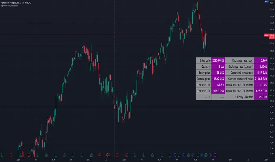
[Kpt-Ahab] PnL-calculatorThe PnL-Cal shows how much you’re up or down in your own currency, based on the current exchange rate.
Let’s say your home currency is EUR.
On October 10, 2022, you bought 10 Tesla stocks at $219 apiece.
Back then, with an exchange rate of 0.9701, you spent €2,257.40.
If you sold the 10 Tesla shares on April 17, 2025 for $241.37 each, that’s around a 10% gain in USD.
But if you converted the USD back to EUR on the same day at an exchange rate of 1.1398, you’d actually end up with an overall loss of about 6.2%.
Right now, only a single entry point is supported.
If you bought shares on different days with different exchange rates, you’ll unfortunately have to enter an average for now.
For viewing on a phone, the table can be simplified.
Trendline Breaks with Multi Fibonacci Supertrend StrategyTMFS Strategy: Advanced Trendline Breakouts with Multi-Fibonacci Supertrend
Elevate your algorithmic trading with institutional-grade signal confluence
Strategy Genesis & Evolution
This advanced trading system represents the culmination of a personal research journey, evolving from my custom " Multi Fibonacci Supertrend with Signals " indicator into a comprehensive trading strategy. Built upon the exceptional trendline detection methodology pioneered by LuxAlgo in their " Trendlines with Breaks " indicator, I've engineered a systematic framework that integrates multiple technical factors into a cohesive trading system.
Core Fibonacci Principles
At the heart of this strategy lies the Fibonacci sequence application to volatility measurement:
// Fibonacci-based factors for multiple Supertrend calculations
factor1 = input.float(0.618, 'Factor 1 (Weak/Fibonacci)', minval = 0.01, step = 0.01)
factor2 = input.float(1.618, 'Factor 2 (Medium/Golden Ratio)', minval = 0.01, step = 0.01)
factor3 = input.float(2.618, 'Factor 3 (Strong/Extended Fib)', minval = 0.01, step = 0.01)
These precise Fibonacci ratios create a dynamic volatility envelope that adapts to changing market conditions while maintaining mathematical harmony with natural price movements.
Dynamic Trendline Detection
The strategy incorporates LuxAlgo's pioneering approach to trendline detection:
// Pivotal swing detection (inspired by LuxAlgo)
pivot_high = ta.pivothigh(swing_length, swing_length)
pivot_low = ta.pivotlow(swing_length, swing_length)
// Dynamic slope calculation using ATR
slope = atr_value / swing_length * atr_multiplier
// Update trendlines based on pivot detection
if bool(pivot_high)
upper_slope := slope
upper_trendline := pivot_high
else
upper_trendline := nz(upper_trendline) - nz(upper_slope)
This adaptive trendline approach automatically identifies key structural market boundaries, adjusting in real-time to evolving chart patterns.
Breakout State Management
The strategy implements sophisticated state tracking for breakout detection:
// Track breakouts with state variables
var int upper_breakout_state = 0
var int lower_breakout_state = 0
// Update breakout state when price crosses trendlines
upper_breakout_state := bool(pivot_high) ? 0 : close > upper_trendline ? 1 : upper_breakout_state
lower_breakout_state := bool(pivot_low) ? 0 : close < lower_trendline ? 1 : lower_breakout_state
// Detect new breakouts (state transitions)
bool new_upper_breakout = upper_breakout_state > upper_breakout_state
bool new_lower_breakout = lower_breakout_state > lower_breakout_state
This state-based approach enables precise identification of the exact moment when price breaks through a significant trendline.
Multi-Factor Signal Confluence
Entry signals require confirmation from multiple technical factors:
// Define entry conditions with multi-factor confluence
long_entry_condition = enable_long_positions and
upper_breakout_state > upper_breakout_state and // New trendline breakout
di_plus > di_minus and // Bullish DMI confirmation
close > smoothed_trend // Price above Supertrend envelope
// Execute trades only with full confirmation
if long_entry_condition
strategy.entry('L', strategy.long, comment = "LONG")
This strict requirement for confluence significantly reduces false signals and improves the quality of trade entries.
Advanced Risk Management
The strategy includes sophisticated risk controls with multiple methodologies:
// Calculate stop loss based on selected method
get_long_stop_loss_price(base_price) =>
switch stop_loss_method
'PERC' => base_price * (1 - long_stop_loss_percent)
'ATR' => base_price - long_stop_loss_atr_multiplier * entry_atr
'RR' => base_price - (get_long_take_profit_price() - base_price) / long_risk_reward_ratio
=> na
// Implement trailing functionality
strategy.exit(
id = 'Long Take Profit / Stop Loss',
from_entry = 'L',
qty_percent = take_profit_quantity_percent,
limit = trailing_take_profit_enabled ? na : long_take_profit_price,
stop = long_stop_loss_price,
trail_price = trailing_take_profit_enabled ? long_take_profit_price : na,
trail_offset = trailing_take_profit_enabled ? long_trailing_tp_step_ticks : na,
comment = "TP/SL Triggered"
)
This flexible approach adapts to varying market conditions while providing comprehensive downside protection.
Performance Characteristics
Rigorous backtesting demonstrates exceptional capital appreciation potential with impressive risk-adjusted metrics:
Remarkable total return profile (1,517%+)
Strong Sortino ratio (3.691) indicating superior downside risk control
Profit factor of 1.924 across all trades (2.153 for long positions)
Win rate exceeding 35% with balanced distribution across varied market conditions
Institutional Considerations
The strategy architecture addresses execution complexities faced by institutional participants with temporal filtering and date-range capabilities:
// Time Filter settings with flexible timezone support
import jason5480/time_filters/5 as time_filter
src_timezone = input.string(defval = 'Exchange', title = 'Source Timezone')
dst_timezone = input.string(defval = 'Exchange', title = 'Destination Timezone')
// Date range filtering for precise execution windows
use_from_date = input.bool(defval = true, title = 'Enable Start Date')
from_date = input.time(defval = timestamp('01 Jan 2022 00:00'), title = 'Start Date')
// Validate trading permission based on temporal constraints
date_filter_approved = time_filter.is_in_date_range(
use_from_date, from_date, use_to_date, to_date, src_timezone, dst_timezone
)
These capabilities enable precise execution timing and market session optimization critical for larger market participants.
Acknowledgments
Special thanks to LuxAlgo for the pioneering work on trendline detection and breakout identification that inspired elements of this strategy. Their innovative approach to technical analysis provided a valuable foundation upon which I could build my Fibonacci-based methodology.
This strategy is shared under the same Attribution-NonCommercial-ShareAlike 4.0 International (CC BY-NC-SA 4.0) license as LuxAlgo's original work.
Past performance is not indicative of future results. Conduct thorough analysis before implementing any algorithmic strategy.

BTC: Open InterestThis indicator tracks the 7-day (default) percentage change in open interest (OI), providing insights into market participation trends. It includes customizable periods and colors, allowing traders to adjust settings for better visualization.
Open interest (OI) is the total number of active contracts (futures or options) that haven’t been closed or settled. It represents the total open positions in the market.
Thus when OI increases, more traders are entering new positions, signaling growing market interest. Conversely, when OI decreases, positions are being closed, suggesting lower trader participation or liquidation.
Attributes & Features:
Open Interest Percentage Change – Measures the 7-day % change in open interest to track market participation.
Customizable Calculation Period – Users can adjust the period (default: 7 days) for more flexible analysis.
Adjustable Colors – Allows modification of colors for better visualization.
Trend Identification – Highlights rising vs. falling open interest trends.
Works Across Assets – Can be used for cryptos, stocks, and futures with open interest data.
Overlay or Separate Panel – Can be plotted on price chart or as a separate indicator.
How It Works:
Fetches Open Interest Data – Retrieves open interest values for each day for USD, USDT, and USDC Bitcoin Perpetual Derivitives.
Calculates Percentage Change – Compares current open interest to its value X days ago (Default = 7 days).
Standard Deviation – Applies standard deviation ranging from -2 to +2 deviations to identify large shifts in OI.
Visual Alerts – Can highlight extreme increases or decreases signaling potential market shifts.
NOTE: THE INDICATOR DATA ONLY GOES BACK TO START OF 2022
Market Crashes & Recessions (1907-Present)Included Recession Periods:
Panic of 1907 (1907–1908)
Post-WWI Recession (1918–1919)
Great Depression (1929–1933)
1937–1938 Recession
1953, 1957, & 1973 Oil Crises Recessions
Early 1980s Recession (1980–1982)
Early 1990s Recession (1990–1991)
Dot-com Bubble (2000–2002)
Global Financial Crisis (2007–2009)
COVID-19 Recession (2020)
2022 Market Correction

MM Labelled AVWAPTradingView provides a tool to show anchored VWAP plots on your screen, but there is no way to label the plots to add additional context to the level. Instead, users are forced to use the plot style (color, line style, line thickness, etc) to indicate what the plots are for and then they have to remember that meaning when looking at different charts. It also means that for key market-wide moments, users will need to add the plot for every symbol.
Now, for the first time on TradingView, you can create anchored VWAP plots with labels on them so you can understand the meaning behind the key moments you care about and don't need to remember what they mean by using styles like color or thickness. You can use this indicator to track key moments like the 2022 market bottom, or the Aug 9, 2024 "Carry Trade Unwind" bottom. The labelled AVWAP plots are visible on every chart by default. If you have an AVWAP moment that is only relevant to a small number of symbols, you can configure the indicator to only appear on those symbols.

Kalman Filter Trend BreakersThe Kalman filter is a recursive algorithm developed in 1960 by Rudolf E. Kálmán, a Hungarian-American engineer and mathematician, that provides optimal estimates of a system's state by combining noisy measurements with a predictive model. It is widely used in control systems, signal processing, and finance for tracking and forecasting.
In trading, KF might be a good replacement for a moving average, as it reacts to price changes in a different way. Not only it follows price direction, but can also track the velocity of price change. This specific behaviour of KF is used in this indicator to track changes in trends.
Trend is characterized by price moving directionally, however, any trend comes to pause or complete stop and reversal, as the price changes more slowly (a trend fades into a sideways movement for a while) or the price movement changes direction, thus making a reversal.
This indicator detects the points where such changes occur (trend breaker points), and produces signals, which serve as points of current trend pausing or reversing. By applying different settings for KF calculation, you can produce less or more signals that indicate change in trend character, and either detect only significant trends changes, or less and shorter trends changes as well.
The signals do not differentiate the exact type of a trend change (it can be a brief trend pause followed by a continuation, as well as a complete reversal). However, once you are in a trend, the significant velocity change indicates a change in trend structure. In this sense, trend breaker signals should not be followed blindly, and can be used only as trend (and subsequently, position) exit confirmations, but not the entry contrarian confirmations.
For better visual representation, you can use chart signals attached to bars, and additionally paint a vertical gradient at each signal which shows significant trend deceleration.
Kalman filter calculations used in this indicator are partially based on an open-source code from @loxx which was published in 2022 as Kalman filter overlay .

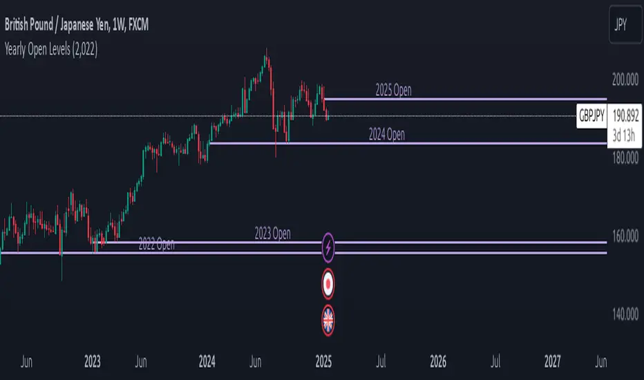
Yearly Open LevelsThe Yearly Open Levels indicator is designed to help traders visualize the opening price of each year on a price chart.
Key Features:
Yearly Open Display: Automatically calculates and displays the opening price for each year starting from a user-defined starting year. This helps traders quickly spot where the price opens each year.
Customizable Start Year: Users can set a specific year to begin displaying opening levels. The default starting year is 2022, but this can be adjusted based on individual trader needs.
Visual Lines and Labels: Each yearly open is represented by a horizontal line that extends to the right of the chart, making it easy to see the level throughout the year.
A label is placed next to the line, indicating the year and the opening price, enhancing clarity and reference while analyzing price movements.
Color Customization: Traders can choose the color of the lines and labels to fit their charting style or preferences, enhancing the visual representation on different market charts.
Salience Theory Crypto Returns (AiBitcoinTrend)The Salience Theory Crypto Returns Indicator is a sophisticated tool rooted in behavioral finance, designed to identify trading opportunities in the cryptocurrency market. Based on research by Bordalo et al. (2012) and extended by Cai and Zhao (2022), it leverages salience theory—the tendency of investors, particularly retail traders, to overemphasize standout returns.
In the crypto market, dominated by sentiment-driven retail investors, salience effects are amplified. Attention disproportionately focused on certain cryptocurrencies often leads to temporary price surges, followed by reversals as the market stabilizes. This indicator quantifies these effects using a relative return salience measure, enabling traders to capitalize on price reversals and trends, offering a clear edge in navigating the volatile crypto landscape.
👽 How the Indicator Works
Salience Measure Calculation :
👾 The indicator calculates how much each cryptocurrency's return deviates from the average return of all cryptos over the selected ranking period (e.g., 21 days).
👾 This deviation is the salience measure.
👾 The more a return stands out (salient outcome), the higher the salience measure.
Ranking:
👾 Cryptos are ranked in ascending order based on their salience measures.
👾 Rank 1 (lowest salience) means the crypto is closer to the average return and is more predictable.
👾 Higher ranks indicate greater deviation and unpredictability.
Color Interpretation:
👾 Green: Low salience (closer to average) – Trending or Predictable.
👾 Red/Orange: High salience (far from average) – Overpriced/Unpredictable.
👾 Text Gradient (Teal to Light Blue): Helps visualize potential opportunities for mean reversion trades (i.e., cryptos that may return to equilibrium).
👽 Core Features
Salience Measure Calculation
The indicator calculates the salience measure for each cryptocurrency by evaluating how much its return deviates from the average market return over a user-defined ranking period. This measure helps identify which assets are trending predictably and which are likely to experience a reversal.
Dynamic Ranking System
Cryptocurrencies are dynamically ranked based on their salience measures. The ranking helps differentiate between:
Low Salience Cryptos (Green): These are trending or predictable assets.
High Salience Cryptos (Red): These are overpriced or deviating significantly from the average, signaling potential reversals.
👽 Deep Dive into the Core Mathematics
Salience Theory in Action
Salience theory explains how investors, particularly in the crypto market, tend to prefer assets with standout returns (salient outcomes). This behavior often leads to overpricing of assets with high positive returns and underpricing of those with standout negative returns. The indicator captures these deviations to anticipate mean reversions or trend continuations.
Salience Measure Calculation
// Calculate the average return
avgReturn = array.avg(returns)
// Calculate salience measure for each symbol
salienceMeasures = array.new_float()
for i = 0 to array.size(returns) - 1
ret = array.get(returns, i)
salienceMeasure = math.abs(ret - avgReturn) / (math.abs(ret) + math.abs(avgReturn) + 0.1)
array.push(salienceMeasures, salienceMeasure)
Dynamic Ranking
Cryptos are ranked in ascending order based on their salience measures:
Low Ranks: Cryptos with low salience (predictable, trending).
High Ranks: Cryptos with high salience (unpredictable, likely to revert).
👽 Applications
👾 Trend Identification
Identify cryptocurrencies that are currently trending with low salience measures (green). These assets are likely to continue their current direction, making them good candidates for trend-following strategies.
👾 Mean Reversion Trading
Cryptos with high salience measures (red to light blue) may be poised for a mean reversion. These assets are likely to correct back towards the market average.
👾 Reversal Signals
Anticipate potential reversals by focusing on high-ranked cryptos (red). These assets exhibit significant deviation and are prone to price corrections.
👽 Why It Works in Crypto
The cryptocurrency market is dominated by retail investors prone to sentiment-driven behavior. This leads to exaggerated price movements, making the salience effect a powerful predictor of reversals.
👽 Indicator Settings
👾 Ranking Period : Number of bars used to calculate the average return and salience measure.
Higher Values: Smooth out short-term volatility.
Lower Values: Make the ranking more sensitive to recent price movements.
👾 Number of Quantiles : Divide ranked assets into quantile groups (e.g., quintiles).
Higher Values: More detailed segmentation (deciles, percentiles).
Lower Values: Broader grouping (quintiles, quartiles).
👾 Portfolio Percentage : Percentage of the portfolio allocated to each selected asset.
Enter a percentage (e.g., 20 for 20%), automatically converted to a decimal (e.g., 0.20).
Disclaimer: This information is for entertainment purposes only and does not constitute financial advice. Please consult with a qualified financial advisor before making any investment decisions.

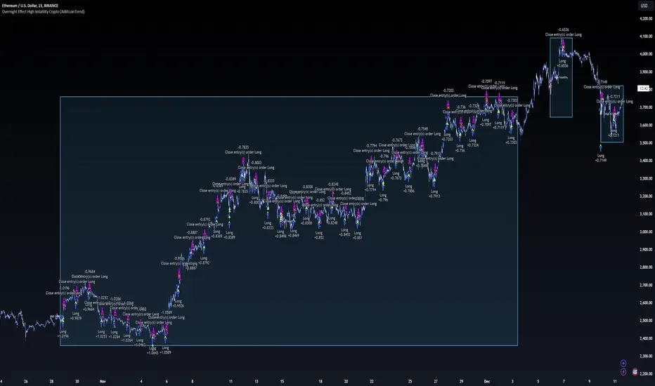
Overnight Effect High Volatility Crypto (AiBitcoinTrend)👽 Overview of the Strategy
This strategy leverages the overnight effect in the cryptocurrency market, specifically targeting the two-hour window from 21:00 UTC to 23:00 UTC. The strategy is designed to be applied only during periods of high volatility, which is determined using historical volatility data. This approach, inspired by research from Padyšák and Vojtko (2022), aims to capitalize on statistically significant return patterns observed during these hours.
Deep Backtesting with a High Volatility Filter
Deep Backtesting without a High Volatility Filter
👽 How the Strategy Works
Volatility Calculation:
Each day at 00:00 UTC, the strategy calculates the 30-day historical volatility of crypto returns (typically Bitcoin). The historical volatility is the standard deviation of the log returns over the past 30 days, representing the market's recent volatility level.
Median Volatility Benchmark:
The median of the 30-day historical volatility is calculated over a 365-day period (one year). This median acts as a benchmark to classify each day as either:
👾 High Volatility: When the current 30-day volatility exceeds the median volatility.
👾 Low Volatility: When the current 30-day volatility is below the median.
Trading Rule:
If the day is classified as a High Volatility Day, the strategy executes the following trades:
👾 Buy at 21:00 UTC.
👾 Sell at 23:00 UTC.
Trade Execution Details:
The strategy uses a 0.02% fee per trade.
Each trade is executed with 25% of the available capital. This allocation helps manage risk while allowing for compounding returns.
Rationale:
The returns during the 22:00 and 23:00 UTC hours have been found to be statistically significant during high volatility periods. The overnight effect is believed to drive this phenomenon due to the asynchronous closing hours of global financial markets. This creates unique trading opportunities in the cryptocurrency market, where exchanges remain open 24/7.
👽 Market Context and Global Time Zone Impact
👾 Why 21:00 to 23:00 UTC?
During this window, major traditional financial markets are closed:
NYSE (New York) closes at 21:00 UTC.
London and European markets are closed during these hours.
Asian markets (Tokyo, Hong Kong, etc.) open later, leaving this window largely unaffected by traditional trading flows.
This global market inactivity creates a period where significant moves can occur in the cryptocurrency market, particularly during high volatility.
👽 Strategy Parameters
Volatility Period: 30 days.
The lookback period for calculating historical volatility.
Median Period: 365 days.
The lookback period for calculating the median volatility benchmark.
Entry Time: 21:00 UTC.
Adjust this to your local time if necessary (e.g., 16:00 in New York, 22:00 in Stockholm).
Exit Time: 23:00 UTC.
Adjust this to your local time if necessary (e.g., 18:00 in New York, 00:00 midnight in Stockholm).
👽 Benefits of the Strategy
Seasonality Effect:
The strategy captures consistent patterns driven by the overnight effect and high volatility periods.
Risk Reduction:
Since trades are executed during a specific window and only on high volatility days, the strategy helps mitigate exposure to broader market risk.
Simplicity and Efficiency:
The strategy is moderately complex, making it accessible for traders while offering significant returns.
Global Applicability:
Suitable for traders worldwide, with clear guidelines on adjusting for local time zones.
👽 Considerations
Market Conditions: The strategy works best in a high-volatility environment.
Execution: Requires precise timing to enter and exit trades at the specified hours.
Time Zone Adjustments: Ensure you convert UTC times accurately based on your location to execute trades at the correct local times.
Disclaimer: This information is for entertainment purposes only and does not constitute financial advice. Please consult with a qualified financial advisor before making any investment decisions.
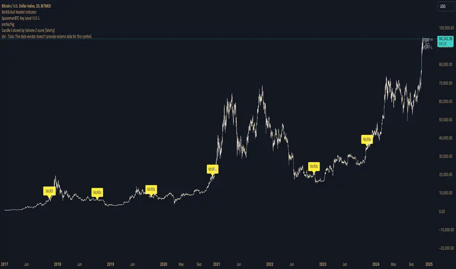
McRib Bull Market Indicator# McRib Bull Market Indicator
## Overview
The McRib Bull Market Indicator is a unique technical analysis tool that marks McDonald's McRib sandwich release dates on your trading charts. While seemingly unconventional, this indicator serves as a fascinating historical reference point for market analysis, particularly for studying periods of market expansion.
## Key Features
- Visual yellow labels marking verified McRib release dates from 2012 to 2024
- Clean, unobtrusive design that overlays on any chart timeframe
- Covers both U.S. and international releases (including UK and Australia)
## Historical Reference Points
The indicator includes release dates from:
- December 2012
- October-December 2014
- January 2015
- October 2016
- November 2017
- October 2018
- October 2019
- December 2020
- October 2022
- November 2023
- December 2024
## Usage Guide
1. Add the indicator to any chart by searching for "McRib Bull Market Indicator"
2. The indicator will automatically display yellow labels above price candles on McRib release dates
3. Use these reference points to:
- Analyze market conditions during McRib releases
- Study potential correlations between releases and market movements
- Compare market behavior across different McRib release periods
- Identify any patterns in market expansion phases coinciding with releases
## Trading Application
While initially created as a novelty indicator, it can be used to:
- Mark specific historical points of reference for broader market analysis
- Study potential market psychology around major promotional events
- Compare seasonal market patterns with recurring release dates
- Analyze market expansion phases that coincide with releases
Remember: While this indicator provides interesting historical reference points, it should be used as part of a comprehensive trading strategy rather than as a standalone trading signal.
Trading IQ - ICT LibraryLibrary "ICTlibrary"
Used to calculate various ICT related price levels and strategies. An ongoing project.
Hello Coders!
This library is meant for sourcing ICT related concepts. While some functions might generate more output than you require, you can specify "Lite Mode" as "true" in applicable functions to slim down necessary inputs.
isLastBar(userTF)
Identifies the last bar on the chart before a timeframe change
Parameters:
userTF (simple int) : the timeframe you wish to calculate the last bar for, must be converted to integer using 'timeframe.in_seconds()'
Returns: bool true if bar on chart is last bar of higher TF, dalse if bar on chart is not last bar of higher TF
necessaryData(atrTF)
returns necessaryData UDT for historical data access
Parameters:
atrTF (float) : user-selected timeframe ATR value.
Returns: logZ. log return Z score, used for calculating order blocks.
method gradBoxes(gradientBoxes, idColor, timeStart, bottom, top, rightCoordinate)
creates neon like effect for box drawings
Namespace types: array
Parameters:
gradientBoxes (array) : an array.new() to store the gradient boxes
idColor (color)
timeStart (int) : left point of box
bottom (float) : bottom of box price point
top (float) : top of box price point
rightCoordinate (int) : right point of box
Returns: void
checkIfTraded(tradeName)
checks if recent trade is of specific name
Parameters:
tradeName (string)
Returns: bool true if recent trade id matches target name, false otherwise
checkIfClosed(tradeName)
checks if recent closed trade is of specific name
Parameters:
tradeName (string)
Returns: bool true if recent closed trade id matches target name, false otherwise
IQZZ(atrMult, finalTF)
custom ZZ to quickly determine market direction.
Parameters:
atrMult (float) : an atr multiplier used to determine the required price move for a ZZ direction change
finalTF (string) : the timeframe used for the atr calcuation
Returns: dir market direction. Up => 1, down => -1
method drawBos(id, startPoint, getKeyPointTime, getKeyPointPrice, col, showBOS, isUp)
calculates and draws Break Of Structure
Namespace types: array
Parameters:
id (array)
startPoint (chart.point)
getKeyPointTime (int) : the actual time of startPoint, simplystartPoint.time
getKeyPointPrice (float) : the actual time of startPoint, simplystartPoint.price
col (color) : color of the BoS line / label
showBOS (bool) : whether to show label/line. This function still calculates internally for other ICT related concepts even if not drawn.
isUp (bool) : whether BoS happened during price increase or price decrease.
Returns: void
method drawMSS(id, startPoint, getKeyPointTime, getKeyPointPrice, col, showMSS, isUp, upRejections, dnRejections, highArr, lowArr, timeArr, closeArr, openArr, atrTFarr, upRejectionsPrices, dnRejectionsPrices)
calculates and draws Market Structure Shift. This data is also used to calculate Rejection Blocks.
Namespace types: array
Parameters:
id (array)
startPoint (chart.point)
getKeyPointTime (int) : the actual time of startPoint, simplystartPoint.time
getKeyPointPrice (float) : the actual time of startPoint, simplystartPoint.price
col (color) : color of the MSS line / label
showMSS (bool) : whether to show label/line. This function still calculates internally for other ICT related concepts even if not drawn.
isUp (bool) : whether MSS happened during price increase or price decrease.
upRejections (array)
dnRejections (array)
highArr (array) : array containing historical highs, should be taken from the UDT "necessaryData" defined above
lowArr (array) : array containing historical lows, should be taken from the UDT "necessaryData" defined above
timeArr (array) : array containing historical times, should be taken from the UDT "necessaryData" defined above
closeArr (array) : array containing historical closes, should be taken from the UDT "necessaryData" defined above
openArr (array) : array containing historical opens, should be taken from the UDT "necessaryData" defined above
atrTFarr (array) : array containing historical atr values (of user-selected TF), should be taken from the UDT "necessaryData" defined above
upRejectionsPrices (array) : array containing up rejections prices. Is sorted and used to determine selective looping for invalidations.
dnRejectionsPrices (array) : array containing down rejections prices. Is sorted and used to determine selective looping for invalidations.
Returns: void
method getTime(id, compare, timeArr)
gets time of inputted price (compare) in an array of data
this is useful when the user-selected timeframe for ICT concepts is greater than the chart's timeframe
Namespace types: array
Parameters:
id (array) : the array of data to search through, to find which index has the same value as "compare"
compare (float) : the target data point to find in the array
timeArr (array) : array of historical times
Returns: the time that the data point in the array was recorded
method OB(id, highArr, signArr, lowArr, timeArr, sign)
store bullish orderblock data
Namespace types: array
Parameters:
id (array)
highArr (array) : array of historical highs
signArr (array) : array of historical price direction "math.sign(close - open)"
lowArr (array) : array of historical lows
timeArr (array) : array of historical times
sign (int) : orderblock direction, -1 => bullish, 1 => bearish
Returns: void
OTEstrat(OTEstart, future, closeArr, highArr, lowArr, timeArr, longOTEPT, longOTESL, longOTElevel, shortOTEPT, shortOTESL, shortOTElevel, structureDirection, oteLongs, atrTF, oteShorts)
executes the OTE strategy
Parameters:
OTEstart (chart.point)
future (int) : future time point for drawings
closeArr (array) : array of historical closes
highArr (array) : array of historical highs
lowArr (array) : array of historical lows
timeArr (array) : array of historical times
longOTEPT (string) : user-selected long OTE profit target, please create an input.string() for this using the example below
longOTESL (int) : user-selected long OTE stop loss, please create an input.string() for this using the example below
longOTElevel (float) : long entry price of selected retracement ratio for OTE
shortOTEPT (string) : user-selected short OTE profit target, please create an input.string() for this using the example below
shortOTESL (int) : user-selected short OTE stop loss, please create an input.string() for this using the example below
shortOTElevel (float) : short entry price of selected retracement ratio for OTE
structureDirection (string) : current market structure direction, this should be "Up" or "Down". This is used to cancel pending orders if market structure changes
oteLongs (bool) : input.bool() for whether OTE longs can be executed
atrTF (float) : atr of the user-seleceted TF
oteShorts (bool) : input.bool() for whether OTE shorts can be executed
@exampleInputs
oteLongs = input.bool(defval = false, title = "OTE Longs", group = "Optimal Trade Entry")
longOTElevel = input.float(defval = 0.79, title = "Long Entry Retracement Level", options = , group = "Optimal Trade Entry")
longOTEPT = input.string(defval = "-0.5", title = "Long TP", options = , group = "Optimal Trade Entry")
longOTESL = input.int(defval = 0, title = "How Many Ticks Below Swing Low For Stop Loss", group = "Optimal Trade Entry")
oteShorts = input.bool(defval = false, title = "OTE Shorts", group = "Optimal Trade Entry")
shortOTElevel = input.float(defval = 0.79, title = "Short Entry Retracement Level", options = , group = "Optimal Trade Entry")
shortOTEPT = input.string(defval = "-0.5", title = "Short TP", options = , group = "Optimal Trade Entry")
shortOTESL = input.int(defval = 0, title = "How Many Ticks Above Swing Low For Stop Loss", group = "Optimal Trade Entry")
Returns: void (0)
displacement(logZ, atrTFreg, highArr, timeArr, lowArr, upDispShow, dnDispShow, masterCoords, labelLevels, dispUpcol, rightCoordinate, dispDncol, noBorders)
calculates and draws dispacements
Parameters:
logZ (float) : log return of current price, used to determine a "significant price move" for a displacement
atrTFreg (float) : atr of user-seleceted timeframe
highArr (array) : array of historical highs
timeArr (array) : array of historical times
lowArr (array) : array of historical lows
upDispShow (int) : amount of historical upside displacements to show
dnDispShow (int) : amount of historical downside displacements to show
masterCoords (map) : a map to push the most recent displacement prices into, useful for having key levels in one data structure
labelLevels (string) : used to determine label placement for the displacement, can be inside box, outside box, or none, example below
dispUpcol (color) : upside displacement color
rightCoordinate (int) : future time for displacement drawing, best is "last_bar_time"
dispDncol (color) : downside displacement color
noBorders (bool) : input.bool() to remove box borders, example below
@exampleInputs
labelLevels = input.string(defval = "Inside" , title = "Box Label Placement", options = )
noBorders = input.bool(defval = false, title = "No Borders On Levels")
Returns: void
method getStrongLow(id, startIndex, timeArr, lowArr, strongLowPoints)
unshift strong low data to array id
Namespace types: array
Parameters:
id (array)
startIndex (int) : the starting index for the timeArr array of the UDT "necessaryData".
this point should start from at least 1 pivot prior to find the low before an upside BoS
timeArr (array) : array of historical times
lowArr (array) : array of historical lows
strongLowPoints (array) : array of strong low prices. Used to retrieve highest strong low price and see if need for
removal of invalidated strong lows
Returns: void
method getStrongHigh(id, startIndex, timeArr, highArr, strongHighPoints)
unshift strong high data to array id
Namespace types: array
Parameters:
id (array)
startIndex (int) : the starting index for the timeArr array of the UDT "necessaryData".
this point should start from at least 1 pivot prior to find the high before a downside BoS
timeArr (array) : array of historical times
highArr (array) : array of historical highs
strongHighPoints (array)
Returns: void
equalLevels(highArr, lowArr, timeArr, rightCoordinate, equalHighsCol, equalLowsCol, liteMode)
used to calculate recent equal highs or equal lows
Parameters:
highArr (array) : array of historical highs
lowArr (array) : array of historical lows
timeArr (array) : array of historical times
rightCoordinate (int) : a future time (right for boxes, x2 for lines)
equalHighsCol (color) : user-selected color for equal highs drawings
equalLowsCol (color) : user-selected color for equal lows drawings
liteMode (bool) : optional for a lite mode version of an ICT strategy. For more control over drawings leave as "True", "False" will apply neon effects
Returns: void
quickTime(timeString)
used to quickly determine if a user-inputted time range is currently active in NYT time
Parameters:
timeString (string) : a time range
Returns: true if session is active, false if session is inactive
macros(showMacros, noBorders)
used to calculate and draw session macros
Parameters:
showMacros (bool) : an input.bool() or simple bool to determine whether to activate the function
noBorders (bool) : an input.bool() to determine whether the box anchored to the session should have borders
Returns: void
po3(tf, left, right, show)
use to calculate HTF po3 candle
@tip only call this function on "barstate.islast"
Parameters:
tf (simple string)
left (int) : the left point of the candle, calculated as bar_index + left,
right (int) : :the right point of the candle, calculated as bar_index + right,
show (bool) : input.bool() whether to show the po3 candle or not
Returns: void
silverBullet(silverBulletStratLong, silverBulletStratShort, future, userTF, H, L, H2, L2, noBorders, silverBulletLongTP, historicalPoints, historicalData, silverBulletLongSL, silverBulletShortTP, silverBulletShortSL)
used to execute the Silver Bullet Strategy
Parameters:
silverBulletStratLong (simple bool)
silverBulletStratShort (simple bool)
future (int) : a future time, used for drawings, example "last_bar_time"
userTF (simple int)
H (float) : the high price of the user-selected TF
L (float) : the low price of the user-selected TF
H2 (float) : the high price of the user-selected TF
L2 (float) : the low price of the user-selected TF
noBorders (bool) : an input.bool() used to remove the borders from box drawings
silverBulletLongTP (series silverBulletLevels)
historicalPoints (array)
historicalData (necessaryData)
silverBulletLongSL (series silverBulletLevels)
silverBulletShortTP (series silverBulletLevels)
silverBulletShortSL (series silverBulletLevels)
Returns: void
method invalidFVGcheck(FVGarr, upFVGpricesSorted, dnFVGpricesSorted)
check if existing FVGs are still valid
Namespace types: array
Parameters:
FVGarr (array)
upFVGpricesSorted (array) : an array of bullish FVG prices, used to selective search through FVG array to remove invalidated levels
dnFVGpricesSorted (array) : an array of bearish FVG prices, used to selective search through FVG array to remove invalidated levels
Returns: void (0)
method drawFVG(counter, FVGshow, FVGname, FVGcol, data, masterCoords, labelLevels, borderTransp, liteMode, rightCoordinate)
draws FVGs on last bar
Namespace types: map
Parameters:
counter (map) : a counter, as map, keeping count of the number of FVGs drawn, makes sure that there aren't more FVGs drawn
than int FVGshow
FVGshow (int) : the number of FVGs to show. There should be a bullish FVG show and bearish FVG show. This function "drawFVG" is used separately
for bearish FVG and bullish FVG.
FVGname (string) : the name of the FVG, "FVG Up" or "FVG Down"
FVGcol (color) : desired FVG color
data (FVG)
masterCoords (map) : a map containing the names and price points of key levels. Used to define price ranges.
labelLevels (string) : an input.string with options "Inside", "Outside", "Remove". Determines whether FVG labels should be inside box, outside,
or na.
borderTransp (int)
liteMode (bool)
rightCoordinate (int) : the right coordinate of any drawings. Must be a time point.
Returns: void
invalidBlockCheck(bullishOBbox, bearishOBbox, userTF)
check if existing order blocks are still valid
Parameters:
bullishOBbox (array) : an array declared using the UDT orderBlock that contains bullish order block related data
bearishOBbox (array) : an array declared using the UDT orderBlock that contains bearish order block related data
userTF (simple int)
Returns: void (0)
method lastBarRejections(id, rejectionColor, idShow, rejectionString, labelLevels, borderTransp, liteMode, rightCoordinate, masterCoords)
draws rejectionBlocks on last bar
Namespace types: array
Parameters:
id (array) : the array, an array of rejection block data declared using the UDT rejection block
rejectionColor (color) : the desired color of the rejection box
idShow (int)
rejectionString (string) : the desired name of the rejection blocks
labelLevels (string) : an input.string() to determine if labels for the block should be inside the box, outside, or none.
borderTransp (int)
liteMode (bool) : an input.bool(). True = neon effect, false = no neon.
rightCoordinate (int) : atime for the right coordinate of the box
masterCoords (map) : a map that stores the price of key levels and assigns them a name, used to determine price ranges
Returns: void
method OBdraw(id, OBshow, BBshow, OBcol, BBcol, bullishString, bearishString, isBullish, labelLevels, borderTransp, liteMode, rightCoordinate, masterCoords)
draws orderblocks and breaker blocks for data stored in UDT array()
Namespace types: array
Parameters:
id (array) : the array, an array of order block data declared using the UDT orderblock
OBshow (int) : the number of order blocks to show
BBshow (int) : the number of breaker blocks to show
OBcol (color) : color of order blocks
BBcol (color) : color of breaker blocks
bullishString (string) : the title of bullish blocks, which is a regular bullish orderblock or a bearish orderblock that's converted to breakerblock
bearishString (string) : the title of bearish blocks, which is a regular bearish orderblock or a bullish orderblock that's converted to breakerblock
isBullish (bool) : whether the array contains bullish orderblocks or bearish orderblocks. If bullish orderblocks,
the array will naturally contain bearish BB, and if bearish OB, the array will naturally contain bullish BB
labelLevels (string) : an input.string() to determine if labels for the block should be inside the box, outside, or none.
borderTransp (int)
liteMode (bool) : an input.bool(). True = neon effect, false = no neon.
rightCoordinate (int) : atime for the right coordinate of the box
masterCoords (map) : a map that stores the price of key levels and assigns them a name, used to determine price ranges
Returns: void
FVG
UDT for FVG calcualtions
Fields:
H (series float) : high price of user-selected timeframe
L (series float) : low price of user-selected timeframe
direction (series string) : FVG direction => "Up" or "Down"
T (series int) : => time of bar on user-selected timeframe where FVG was created
fvgLabel (series label) : optional label for FVG
fvgLineTop (series line) : optional line for top of FVG
fvgLineBot (series line) : optional line for bottom of FVG
fvgBox (series box) : optional box for FVG
labelLine
quickly pair a line and label together as UDT
Fields:
lin (series line) : Line you wish to pair with label
lab (series label) : Label you wish to pair with line
orderBlock
UDT for order block calculations
Fields:
orderBlockData (array) : array containing order block x and y points
orderBlockBox (series box) : optional order block box
vioCount (series int) : = 0 violation count of the order block. 0 = Order Block, 1 = Breaker Block
traded (series bool)
status (series string) : = "OB" status == "OB" => Level is order block. status == "BB" => Level is breaker block.
orderBlockLab (series label) : options label for the order block / breaker block.
strongPoints
UDT for strong highs and strong lows
Fields:
price (series float) : price of the strong high or strong low
timeAtprice (series int) : time of the strong high or strong low
strongPointLabel (series label) : optional label for strong point
strongPointLine (series line) : optional line for strong point
overlayLine (series line) : optional lines for strong point to enhance visibility
overlayLine2 (series line) : optional lines for strong point to enhance visibility
displacement
UDT for dispacements
Fields:
highPrice (series float) : high price of displacement
lowPrice (series float) : low price of displacement
timeAtPrice (series int) : time of bar where displacement occurred
displacementBox (series box) : optional box to draw displacement
displacementLab (series label) : optional label for displacement
po3data
UDT for po3 calculations
Fields:
dHigh (series float) : higher timeframe high price
dLow (series float) : higher timeframe low price
dOpen (series float) : higher timeframe open price
dClose (series float) : higher timeframe close price
po3box (series box) : box to draw po3 candle body
po3line (array) : line array to draw po3 wicks
po3Labels (array) : label array to label price points of po3 candle
macros
UDT for session macros
Fields:
sessions (array) : Array of sessions, you can populate this array using the "quickTime" function located above "export macros".
prices (matrix) : Matrix of session data -> open, high, low, close, time
sessionTimes (array) : Array of session names. Pairs with array sessions.
sessionLines (matrix) : Optional array for sesion drawings.
OTEtimes
UDT for data storage and drawings associated with OTE strategy
Fields:
upTimes (array) : time of highest point before trade is taken
dnTimes (array) : time of lowest point before trade is taken
tpLineLong (series line) : line to mark tp level long
tpLabelLong (series label) : label to mark tp level long
slLineLong (series line) : line to mark sl level long
slLabelLong (series label) : label to mark sl level long
tpLineShort (series line) : line to mark tp level short
tpLabelShort (series label) : label to mark tp level short
slLineShort (series line) : line to mark sl level short
slLabelShort (series label) : label to mark sl level short
sweeps
UDT for data storage and drawings associated with liquidity sweeps
Fields:
upSweeps (matrix) : matrix containing liquidity sweep price points and time points for up sweeps
dnSweeps (matrix) : matrix containing liquidity sweep price points and time points for down sweeps
upSweepDrawings (array) : optional up sweep box array. Pair the size of this array with the rows or columns,
dnSweepDrawings (array) : optional up sweep box array. Pair the size of this array with the rows or columns,
raidExitDrawings
UDT for drawings associated with the Liquidity Raid Strategy
Fields:
tpLine (series line) : tp line for the liquidity raid entry
tpLabel (series label) : tp label for the liquidity raid entry
slLine (series line) : sl line for the liquidity raid entry
slLabel (series label) : sl label for the liquidity raid entry
m2022
UDT for data storage and drawings associated with the Model 2022 Strategy
Fields:
mTime (series int) : time of the FVG where entry limit order is placed
mIndex (series int) : array index of FVG where entry limit order is placed. This requires an array of FVG data, which is defined above.
mEntryDistance (series float) : the distance of the FVG to the 50% range. M2022 looks for the fvg closest to 50% mark of range.
mEntry (series float) : the entry price for the most eligible fvg
fvgHigh (series float) : the high point of the eligible fvg
fvgLow (series float) : the low point of the eligible fvg
longFVGentryBox (series box) : long FVG box, used to draw the eligible FVG
shortFVGentryBox (series box) : short FVG box, used to draw the eligible FVG
line50P (series line) : line used to mark 50% of the range
line100P (series line) : line used to mark 100% (top) of the range
line0P (series line) : line used to mark 0% (bottom) of the range
label50P (series label) : label used to mark 50% of the range
label100P (series label) : label used to mark 100% (top) of the range
label0P (series label) : label used to mark 0% (bottom) of the range
sweepData (array)
silverBullet
UDT for data storage and drawings associated with the Silver Bullet Strategy
Fields:
session (series bool)
sessionStr (series string) : name of the session for silver bullet
sessionBias (series string)
sessionHigh (series float) : = high high of session // use math.max(silverBullet.sessionHigh, high)
sessionLow (series float) : = low low of session // use math.min(silverBullet.sessionLow, low)
sessionFVG (series float) : if applicable, the FVG created during the session
sessionFVGdraw (series box) : if applicable, draw the FVG created during the session
traded (series bool)
tp (series float) : tp of trade entered at the session FVG
sl (series float) : sl of trade entered at the session FVG
sessionDraw (series box) : optional draw session with box
sessionDrawLabel (series label) : optional label session with label
silverBulletDrawings
UDT for trade exit drawings associated with the Silver Bullet Strategy
Fields:
tpLine (series line) : tp line drawing for strategy
tpLabel (series label) : tp label drawing for strategy
slLine (series line) : sl line drawing for strategy
slLabel (series label) : sl label drawing for strategy
unicornModel
UDT for data storage and drawings associated with the Unicorn Model Strategy
Fields:
hPoint (chart.point)
hPoint2 (chart.point)
hPoint3 (chart.point)
breakerBlock (series box) : used to draw the breaker block required for the Unicorn Model
FVG (series box) : used to draw the FVG required for the Unicorn model
topBlock (series float) : price of top of breaker block, can be used to detail trade entry
botBlock (series float) : price of bottom of breaker block, can be used to detail trade entry
startBlock (series int) : start time of the breaker block, used to set the "left = " param for the box
includes (array) : used to store the time of the breaker block, or FVG, or the chart point sequence that setup the Unicorn Model.
entry (series float) : // eligible entry price, for longs"math.max(topBlock, FVG.get_top())",
tpLine (series line) : optional line to mark PT
tpLabel (series label) : optional label to mark PT
slLine (series line) : optional line to mark SL
slLabel (series label) : optional label to mark SL
rejectionBlocks
UDT for data storage and drawings associated with rejection blocks
Fields:
rejectionPoint (chart.point)
bodyPrice (series float) : candle body price closest to the rejection point, for "Up" rejections => math.max(open, close),
rejectionBox (series box) : optional box drawing of the rejection block
rejectionLabel (series label) : optional label for the rejection block
equalLevelsDraw
UDT for data storage and drawings associated with equal highs / equal lows
Fields:
connector (series line) : single line placed at the first high or low, y = avgerage of distinguished equal highs/lows
connectorLab (series label) : optional label to be placed at the highs or lows
levels (array) : array containing the equal highs or lows prices
times (array) : array containing the equal highs or lows individual times
startTime (series int) : the time of the first high or low that forms a sequence of equal highs or lows
radiate (array) : options label to "radiate" the label in connector lab. Can be used for anything
necessaryData
UDT for data storage of historical price points.
Fields:
highArr (array) : array containing historical high points
lowArr (array) : array containing historical low points
timeArr (array) : array containing historical time points
logArr (array) : array containing historical log returns
signArr (array) : array containing historical price directions
closeArr (array) : array containing historical close points
binaryTimeArr (array) : array containing historical time points, uses "push" instead of "unshift" to allow for binary search
binaryCloseArr (array) : array containing historical close points, uses "push" instead of "unshift" to allow the correct
binaryOpenArr (array) : array containing historical optn points, uses "push" instead of "unshift" to allow the correct
atrTFarr (array) : array containing historical user-selected TF atr points
openArr (array) : array containing historical open points

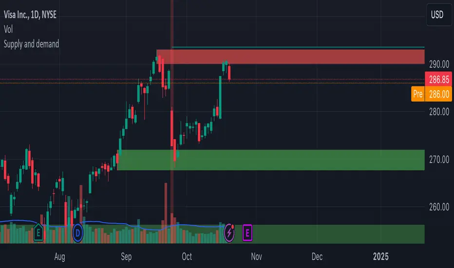
Supply and demandHi all!
This is my take on supply/demand. The gist is that it creates a zone if there is a big enough reaction. This is configurable in settings as "Minimum range (ATR factor)" (the Average True Length of length 14) that is the distance that the price must travel and "Reaction bars" that is the maximum number of bars that price must travel this distance. The zones that are shown are the ones that have a retest, break and retest or is unmitigated (untouched). If a zone is mitigated (entered) or broken it is temporarily hidden. For a zone to be created it needs to have this reaction and the previous bar does not.
So this script will show you zones that are fresh (unmitigated), retested or broken and retested. This means that the zones that are shown have "proven" that they are good zones through this. Basically it means that the script creates a bunch of zones and then picks the good once. This makes the script have some latency, but will hopefully give you good zones. A zone is completely removed if it's broken twice (it's okay if it's broken once and can still have a retest after it has flipped from previous supply (or resistance) into demand (or support)).
Here is a zone (the one that has the lowest opacity) that is broken and retested that could have resulted in a good long trade (the settings are default but has a stop in the beginning of 2024):
You have a setting to remove zones that are pierced (broken by price wicks). The following zone is pierced by price (in the beginning of May) that will not be shown after the start of May if you have "Pierced" checked (the indicator has default settings but a stop in the middle of April):
You have a trend section. Zones that create a reaction upwards can only be created if the trend is considered to be up, and vice versa. The options here are "SMA50" (the current price needs to be over the Simple Moving Average of length 50) and "SMA50, SMA200" (price needs to be over the Simple Moving Average of length 50 and the Simple Moving Average of length 50 needs to be over the Simple Moving Average of length 200). If these conditions are met the trend is considered to be up, otherwise it's down. You can disable this by choosing "No detection".
The zones that are shown also need to be within a limit (of the current price). This limit is 10 (factor of the Average True Range if length 14) by default. Set this to 0 to deactivate. This is useful for not showing zones that are far away from current price and therefore unlikely to be interacted with.
You can stop the calculation of zones (through the "Stop" value in the settings). This is useful to see if previous zones were any good. I used it in my testing of the script but left it because it can be nice to have.
The zones created by the script have different transparency based upon the zone's interaction. The clearest zones are the ones that are unmitigated, the second clearest ones are the ones having a retest and lastly the zones which are most unclear are the ones having a break and then a retest.
You can see the concept of this script to be a mix of supply/demand and support/resistance, having zones being unmitigated (untouched) as the most important but also show the zones having an interaction (in the form of a retest or a break and retest).
This is from a previous supply (or resistance) zone that has flipped into demand (or support) and has shown to be a good zone through a retest followed by a rally (default settings):
This zone has multiple retest and then rallies that could have given a good long trades (it has the default settings but a "Stop" time at 2022-01-14):
TODO:
- Create zones based on pivots
- Handle overlapping zones
- Incorporate volume in the creation and/or interaction with zones
- Add alerts
- Add ability to set maximum zone width
- Add ability to set the maximum number of retest bars
- ...?
The example for this publication has the default settings bit a "Stop" and a tighter "Limit" of 4.
I hope this explanation makes sense, let me know otherwise. Also let me know if you have any suggestions on improvements.
Best of trading luck!
Potential Divergence Checker#### Key Features
1. Potential Divergence Signals:
Potential divergences can signal a change in price movement before it occurs. This indicator identifies potential divergences instead of waiting for full confirmation, allowing it to detect signs of divergence earlier than traditional methods. This provides more flexible entry points and can act as a broader filter for potential setups.
2. Exposing Signals for External Use:
One of its advanced features is the ability to expose signals for use in other scripts. This allows users to integrate divergence signals and related entry/exit points into custom strategies or automated systems.
3. Custom Entry/Exit Timing Based on Years and Days:
The indicator provides entry and exit signals based on years and days, which could be useful for time-specific market behavior, long-term trades, and back testing.
#### Basic Usage
This indicator can check for all types of potential divergences: bullish, hidden bullish, bearish, hidden bearish. All you need to do is choose the type you want to check for under “DIVERGENCE TYPE” in the settings. On the chart, potential bullish divergences will show up as triangles below the price candles. one the chart potential bearish divergences will show up as upside down triangles above the price candles
#### Signals for Advanced Usage
You can use this indicator as a source in other indicators or strategies using the following information:
“ PD: Bull divergence signal ” will return “1” when a divergence is present and “0” when not present
“ PD: HBull divergence(hidden bull) signal ” will return “1” when a divergence is present and “0” when not present
“ PD: Bear divergence signal ” will return “1” when a divergence is present and “0” when not present
“ PD: HBear divergence(hidden bear) signal ” will return “1” when a divergence is present and “0” when not present
“ PD: enter ” signal will return a “1” when both the days and years criteria in the “entry filter settings” are met and “0” when not met.
“ PD: exit ” signal will return a “1” when the days criteria in the “exit filter settings” are met and “0” when not met.
#### Examples of Using Signals
1. If you are testing a long strategy for Bitcoin and do not want it to run during bear market years(e.g., the second year after a US presidential election), you can enable the “year and day filter for entry,” uncheck the following years in the settings: 2010, 2014, 2018, 2022, 2026, and reference the signal below in our strategy
signal: “ PD: enter ”
2. Let’s say you have a good long strategy, but want to make it a bit more profitable, you can tell the strategy not to run on days where there is potential bearish divergence and have it only run on more profitable days using these signals and the appropriate settings in the indicator
signal: “ PD: Bear divergence signal ” will return a ‘0’ with no bearish divergence present
signal: “ PD: enter ” will return a “1” if the entry falls on a specific, more profitable day chosen in the settings
#### Disclaimer
The "Potential Divergence Checker" indicator is a tool designed to identify potential market signals. It may have bugs and not do what it should do. It is not a guarantee of future trading performance, and users should exercise caution when making trading decisions based on its outputs. Always perform your own research and consider consulting with a financial advisor before making any investment decisions. Trading involves significant risk, and past performance is not indicative of future results.
NCI - Timeframe + WatermarkDeveloped by Jayce in June 2022 and later updated by Light in January 2024.
Key Features:
Customizable Watermark: Enhance your chart with a personalized watermark. Enter any text, like your trading mantra or brand name, to keep your focus aligned with your trading strategy.
Adjustable Font Size: Tailor the appearance of your watermark and notes with adjustable font sizes, ranging from "Tiny" to "Huge," ensuring optimal visibility and integration with your chart setup.
Timeframe Display: Stay informed of the current chart's timeframe, neatly displayed alongside your chosen watermark. Whether you're analyzing trends in minutes, hours, or days, this feature keeps you oriented without cluttering your workspace.
Inspirational Note: Complement your watermark with an inspirational note or a quick reminder of your trading discipline and risk management strategies, keeping your principles front and center.

Bitcoin Regression Price BoundariesTLDR
DCA into BTC at or below the blue line. DCA out of BTC when price approaches the red line. There's a setting to toggle the future extrapolation off/on.
INTRODUCTION
Regression analysis is a fundamental and powerful data science tool, when applied CORRECTLY . All Bitcoin regressions I've seen (Rainbow Log, Stock-to-flow, and non-linear models), have glaring flaws ... Namely, that they have huge drift from one cycle to the next.
Presented here, is a canonical application of this statistical tool. "Canonical" meaning that any trained analyst applying the established methodology, would arrive at the same result. We model 3 lines:
Upper price boundary (red) - Predicted the April 2021 top to within 1%
Lower price boundary (green)- Predicted the Dec 2022 bottom within 10%
Non-bubble best fit line (blue) - Last update was performed on Feb 28 2024.
NOTE: The red/green lines were calculated using solely data from BEFORE 2021.
"I'M INTRUIGED, BUT WHAT EXACTLY IS REGRESSION ANALYSIS?"
Quite simply, it attempts to draw a best-fit line over some set of data. As you can imagine, there are endless forms of equations that we might try. So we need objective means of determining which equations are better than others. This is where statistical rigor is crucial.
We check p-values to ensure that a proposed model is better than chance. When comparing two different equations, we check R-squared and Residual Standard Error, to determine which equation is modeling the data better. We check residuals to ensure the equation is sufficiently complex to model all the available signal. We check adjusted R-squared to ensure the equation is not *overly* complex and merely modeling random noise.
While most people probably won't entirely understand the above paragraph, there's enough key terminology in for the intellectually curious to research.
DIVING DEEPER INTO THE 3 REGRESSION LINES ABOVE
WARNING! THIS IS TECHNICAL, AND VERY ABBREVIATED
We prefer a linear regression, as the statistical checks it allows are convenient and powerful. However, the BTCUSD dataset is decidedly non-linear. Thus, we must log transform both the x-axis and y-axis. At the end of this process, we'll use e^ to transform back to natural scale.
Plotting the log transformed data reveals a crucial visual insight. The best fit line for the blowoff tops is different than for the lower price boundary. This is why other models have failed. They attempt to model ALL the data with just one equation. This causes drift in both the upper and lower boundaries. Here we calculate these boundaries as separate equations.
Upper Boundary (in red) = e^(3.24*ln(x)-15.8)
Lower Boundary (green) = e^(0.602*ln^2(x) - 4.78*ln(x) + 7.17)
Non-Bubble best fit (blue) = e^(0.633*ln^2(x) - 5.09*ln(x) +8.12)
* (x) = The number of days since July 18 2010
Anyone familiar with Bitcoin, knows it goes in cycles where price goes stratospheric, typically measured in months; and then a lengthy cool-off period measured in years. The non-bubble best fit line methodically removes the extreme upward deviations until the residuals have the closest statistical semblance to normal data (bell curve shaped data).
Whereas the upper/lower boundary only gets re-calculated in hindsight (well after a blowoff or capitulation occur), the Non-Bubble line changes ever so slightly with each new datapoint. The last update to this line was made on Feb 28, 2024.
ENOUGH NERD TALK! HOW CAN I APPLY THIS?
In the simplest terms, anything below the blue line is a statistical buying opportunity. The closer you approach the green line (the lower boundary) the more statistically strong that opportunity is. As price approaches the red line, is a growing statistical likelyhood/danger of an imminent blowoff top.
So a wise trader would DCA (dollar cost average) into Bitcoin below the blue line; and would DCA out of Bitcoin as it approaches the red line. Historically, you may or may not have a large time-window during points of maximum opportunity. So be vigilant! Anything within 10-20% of the boundary should be regarded as extreme opportunity.
Note: You can toggle the future extrapolation of these lines in the settings (default on).
CLOSING REMARKS
Keep in mind this is a pure statistical analysis. It's likely that this model is probing a complex, real economic process underlying the Bitcoin price. Statistical models like this are most accurate during steady state conditions, where the prevailing fundamentals are stable. (The astute observer will note, that the regression boundaries held despite the economic disruption of 2020).
Thus, it cannot be understated: Should some drastic fundamental change occur in the underlying economic landscape of cryptocurrency, Bitcoin itself, or the broader economy, this model could drastically deviate, and become significantly less accurate.
Furthermore, the upper/lower boundaries cross in the year 2037. THIS MODEL WILL EVENTUALLY BREAK DOWN. But for now, given that Bitcoin price moves on the order of 2000% from bottom to top, it's truly remarkable that, using SOLELY pre-2021 data, this model was able to nail the top/bottom within 10%.
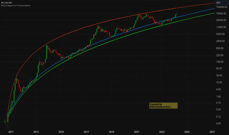
Bitcoin Momentum StrategyThis is a very simple long-only strategy I've used since December 2022 to manage my Bitcoin position.
I'm sharing it as an open-source script for other traders to learn from the code and adapt it to their liking if they find the system concept interesting.
General Overview
Always do your own research and backtesting - this script is not intended to be traded blindly (no script should be) and I've done limited testing on other markets beyond Ethereum and BTC, it's just a template to tweak and play with and make into one's own.
The results shown in the strategy tester are from Bitcoin's inception so as to get a large sample size of trades, and potential returns have diminished significantly as BTC has grown to become a mega cap asset, but the script includes a date filter for backtesting and it has still performed solidly in recent years (speaking from personal experience using it myself - DYOR with the date filter).
The main advantage of this system in my opinion is in limiting the max drawdown significantly versus buy & hodl. Theoretically much better returns can be made by just holding, but that's also a good way to lose 70%+ of your capital in the inevitable bear markets (also speaking from experience).
In saying all of that, the future is fundamentally unknowable and past results in no way guarantee future performance.
System Concept:
Capture as much Bitcoin upside volatility as possible while side-stepping downside volatility as quickly as possible.
The system uses a simple but clever momentum-style trailing stop technique I learned from one of my trading mentors who uses this approach on momentum/trend-following stock market systems.
Basically, the system "ratchets" up the stop-loss to be much tighter during high bearish volatility to protect open profits from downside moves, but loosens the stop loss during sustained bullish momentum to let the position ride.
It is invested most of the time, unless BTC is trading below its 20-week EMA in which case it stays in cash/USDT to avoid holding through bear markets. It only trades one position (no pyramiding) and does not trade short, but can easily be tweaked to do whatever you like if you know what you're doing in Pine.
Default parameters:
HTF: Weekly Chart
EMA: 20-Period
ATR: 5-period
Bar Lookback: 7
Entry Rule #1:
Bitcoin's current price must be trading above its higher-timeframe EMA (Weekly 20 EMA).
Entry Rule #2:
Bitcoin must not be in 'caution' condition (no large bearish volatility swings recently).
Enter at next bar's open if conditions are met and we are not already involved in a trade.
"Caution" Condition:
Defined as true if BTC's recent 7-bar swing high minus current bar's low is > 1.5x ATR, or Daily close < Daily 20-EMA.
Trailing Stop:
Stop is trailed 1 ATR from recent swing high, or 20% of ATR if in caution condition (ie. 0.2 ATR).
Exit on next bar open upon a close below stop loss.
I typically use a limit order to open & exit trades as close to the open price as possible to reduce slippage, but the strategy script uses market orders.
I've never had any issues getting filled on limit orders close to the market price with BTC on the Daily timeframe, but if the exchange has relatively low slippage I've found market orders work fine too without much impact on the results particularly since BTC has consistently remained above $20k and highly liquid.
Cost of Trading:
The script uses no leverage and a default total round-trip commission of 0.3% which is what I pay on my exchange based on their tier structure, but this can vary widely from exchange to exchange and higher commission fees will have a significantly negative impact on realized gains so make sure to always input the correct theoretical commission cost when backtesting any script.
Static slippage is difficult to estimate in the strategy tester given the wide range of prices & liquidity BTC has experienced over the years and it largely depends on position size, I set it to 150 points per buy or sell as BTC is currently very liquid on the exchange I trade and I use limit orders where possible to enter/exit positions as close as possible to the market's open price as it significantly limits my slippage.
But again, this can vary a lot from exchange to exchange (for better or worse) and if BTC volatility is high at the time of execution this can have a negative impact on slippage and therefore real performance, so make sure to adjust it according to your exchange's tendencies.
Tax considerations should also be made based on short-term trade frequency if crypto profits are treated as a CGT event in your region.
Summary:
A simple, but effective and fairly robust system that achieves the goals I set for it.
From my preliminary testing it appears it may also work on altcoins but it might need a bit of tweaking/loosening with the trailing stop distance as the default parameters are designed to work with Bitcoin which obviously behaves very differently to smaller cap assets.
Good luck out there!
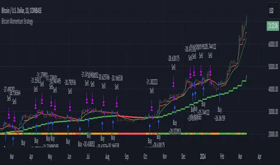
X% Drop in X Days, sold X Days afterIt identifies potential buy signals based on a specified percentage drop in price over a set number of days and calculates the total profit or loss (P/L) over a predefined period. Here's a breakdown of the script and its key parameters:
Script Description:
Indicator Name: "X% Drop in X Days, sold X Days after"
Functionality:
The script signals a buy opportunity when the price of an asset drops by a certain percentage (percentage_drop) within a specified length (length) in days.
It calculates the profit or loss percentage after a set number of days (hold_days) from the buy signal.
The script also displays the cumulative total profit or loss over a specified time frame, from a start date (start_period) to an end date (end_period), which is by default set to the current date.
Display:
Buy signals are marked on the chart.
The profit or loss for each trade after the hold period is displayed.
A label showing the total cumulative profit or loss, along with the start and end dates, is displayed on the chart.
Key Parameters:
percentage_drop (10.0% by default) : The percentage decrease in price that triggers a buy signal. It represents the threshold for the price drop to consider a buying opportunity.
length (3 days by default): The period over which the drop in price is considered. It's the timeframe used to evaluate the percentage drop.
hold_days (30 days by default) : The duration for holding the asset after the buy signal before selling. This parameter defines the time after which the profit or loss is calculated.
start_period (Set to "2022-11-21" by default): The beginning date for calculating the cumulative total profit or loss. This parameter allows the user to define a specific starting point for the analysis.
end_period (Set to the current date by default): The end date for the cumulative total profit or loss calculation. It defaults to the current date but can be set to a specific date for backtesting purposes.
Script Mechanics:
Buy Signal Logic: A buy signal is generated when the closing price is below the highest price of the last 'length' days, adjusted by the 'percentage_drop'.
Profit/Loss Calculation: For each buy signal, the script calculates the profit or loss percentage after 'hold_days' from the purchase. This is displayed on the chart for each trade.
Total P/L Display: The script calculates and displays the cumulative total profit or loss in the defined period (from 'start_period' to 'end_period') in a label on the chart.
Usage:
This script is useful for traders who follow a strategy based on buying assets after significant price drops and holding for a predetermined period. It automates the detection of potential buy opportunities and the calculation of profit or loss, aiding in decision-making and performance analysis.

ICT HTF MSS & Liquidity (fadi)ICT HTF MSS & Liquidity provides higher timeframe view of where the liquidity may reside and when higher timeframe market structure shift has occurred.
In his 2022 mentorship, ICT has advocated used the 15m chart to watch for liquidity and looking for lower timeframes for entry (5m,4m,3m,2m,1m).
Liquidity will reside above pivot points and ICT pivot points are based on 3 candle formation for the short term, three short term formation for intermediate, and three intermediate formation for the long terms.
Options
Timeframe Timeframe to monitor
Use the Short, Intermediate, or Long Term highs and lows
Liquidity Styles
Open liquidity line style, size, and color
Claimed liquidity line style, size, and color
Extend the open liquidity line beyond the current candle
Number of lines to display, this includes claimed and open

VAcc (Velocity & Acceleration)VAcc (Velocity & Acceleration) is a momentum indicator published by Scott Cong in Stocks & Commodities V. 41:09 (8–15). It applies concepts from physics, namely velocity and acceleration, to financial markets. VAcc functions similarly to the popular MACD (Moving Average Convergence Divergence) indicator when using a longer lookback period, but produces more responsive results. With shorter periods, VAcc exhibits characteristics reminiscent of the stochastic oscillator.
🟠 Algorithm
The average velocity over the past n periods is defined as
((C - C_n) / n + (C - C_{n-1}) / (n - 1) + … + (C - C_i) / i + (C - C_1) / 1) / n
At its core, the velocity is a weighted average of the rate of change over the past n periods.
The calculation of the acceleration follows a similar process, where it’s defined as
((V - V_n) / n + (V - V_{n - 1}) / (n - 1) + … + (V - V_i) / i + (V - V_1) / 1) / n
🟠 Comparison with MACD
A comparison of VAcc and MACD on the daily Nasdaq 100 (NDX) chart from August 2022 helps demonstrate VAcc's improved sensitivity. Both indicators utilized a lookback period of 26 days and smoothing of 9 periods.
The VAcc histogram clearly shows a divergence forming, with momentum weakening as prices reached new highs. In contrast, the corresponding MACD histogram significantly lagged in confirming the divergence, highlighting VAcc's ability to identify subtle shifts in trend momentum more immediately than the traditional MACD.

[Library] VAccThis is the library version of VAcc (Velocity & Acceleration), a momentum indicator published by Scott Cong in Stocks & Commodities V. 41:09 (8–15). It applies concepts from physics, namely velocity and acceleration, to financial markets. VAcc functions similarly to the popular MACD (Moving Average Convergence Divergence) indicator when using a longer lookback period, but produces more responsive results. With shorter periods, VAcc exhibits characteristics reminiscent of the stochastic oscillator.
The indicator version of this algorithm is linked below:
🟠 Algorithm
The average velocity over the past n periods is defined as
((C - C_n) / n + (C - C_{n-1}) / (n - 1) + … + (C - C_i) / i + (C - C_1) / 1) / n
At its core, the velocity is a weighted average of the rate of change over the past n periods.
The calculation of the acceleration follows a similar process, where it’s defined as
((V - V_n) / n + (V - V_{n - 1}) / (n - 1) + … + (V - V_i) / i + (V - V_1) / 1) / n
🟠 Comparison with MACD
A comparison of VAcc and MACD on the daily Nasdaq 100 (NDX) chart from August 2022 helps demonstrate VAcc's improved sensitivity. Both indicators utilized a lookback period of 26 days and smoothing of 9 periods.
The VAcc histogram clearly shows a divergence forming, with momentum weakening as prices reached new highs. In contrast, the corresponding MACD histogram significantly lagged in confirming the divergence, highlighting VAcc's ability to identify subtle shifts in trend momentum more immediately than the traditional MACD.
