在腳本中搜尋"4月10日A股市场分析"
10/20/50/100/200 SMA'sMultiple MA's to get a good feel for momentum and interim supports and resistances


Moving Average x10 (SMA, EMA)10 configurable Simple and Exponential moving averages combined in one indicator
SMA RIBBON10 SMA's arranged in a ribbon. Color coded depending on price close. Free to use, open source. As seen in some charts.

10Y Bond Yield Spread (beta)10-Year Bond Yield Spread using Quandl data
See also:
- seekingalpha.com
- www.babypips.com
- www.forexfactory.com

10 Simple & 6 Exponential Moving Averages (w/ 18 day,week,month)* This is for the trader who wants tons of moving averages on their chart from one indicator
* Using the options, you should be able ot turn off some of them if the screen is too noisy for you
* You should also be able to change colors and thickness of the bars
* The thicker bars are for longer term averages
* This version is similar to my other script except it adds the 18 day, 18 week, and 18 Month SMa
* I added them after watching ira Epstein's YouTube videos
* Let me know if there are any bugs or things that need to be change

Hellenic EMA Matrix - PremiumHellenic EMA Matrix - Alpha Omega Premium
Complete User Guide
Table of Contents
Introduction
Indicator Philosophy
Mathematical Constants
EMA Types
Settings
Trading Signals
Visualization
Usage Strategies
FAQ
Introduction
Hellenic EMA Matrix is a premium indicator based on mathematical constants of nature: Phi (Phi - Golden Ratio), Pi (Pi), e (Euler's number). The indicator uses these universal constants to create dynamic EMAs that adapt to the natural rhythms of the market.
Key Features:
6 EMA types based on mathematical constants
Premium visualization with Neon Glow and Gradient Clouds
Automatic Fast/Mid/Slow EMA sorting
STRONG signals for powerful trends
Pulsing Ribbon Bar for instant trend assessment
Works on all timeframes (M1 - MN)
Indicator Philosophy
Why Mathematical Constants?
Traditional EMAs use arbitrary periods (9, 21, 50, 200). Hellenic Matrix goes further, using universal mathematical constants found in nature:
Phi (1.618) - Golden Ratio: galaxy spirals, seashells, human body proportions
Pi (3.14159) - Pi: circles, waves, cycles
e (2.71828) - Natural logarithm base: exponential growth, radioactive decay
Markets are also a natural system composed of millions of participants. Using mathematical constants allows tuning into the natural rhythms of market cycles.
Mathematical Constants
Phi (Phi) - Golden Ratio
Phi = 1.618033988749895
Properties:
Phi² = Phi + 1 = 2.618
Phi³ = 4.236
Phi⁴ = 6.854
Application: Ideal for trending movements and Fibonacci corrections
Pi (Pi) - Pi Number
Pi = 3.141592653589793
Properties:
2Pi = 6.283 (full circle)
3Pi = 9.425
4Pi = 12.566
Application: Excellent for cyclical markets and wave structures
e (Euler) - Euler's Number
e = 2.718281828459045
Properties:
e² = 7.389
e³ = 20.085
e⁴ = 54.598
Application: Suitable for exponential movements and volatile markets
EMA Types
1. Phi (Phi) - Golden Ratio EMA
Description: EMA based on the golden ratio
Period Formula:
Period = Phi^n × Base Multiplier
Parameters:
Phi Power Level (1-8): Power of Phi
Phi¹ = 1.618 → ~16 period (with Base=10)
Phi² = 2.618 → ~26 period
Phi³ = 4.236 → ~42 period (recommended)
Phi⁴ = 6.854 → ~69 period
Recommendations:
Phi² or Phi³ for day trading
Phi⁴ or Phi⁵ for swing trading
Works excellently as Fast EMA
2. Pi (Pi) - Circular EMA
Description: EMA based on Pi for cyclical movements
Period Formula:
Period = Pi × Multiple × Base Multiplier
Parameters:
Pi Multiple (1-10): Pi multiplier
1Pi = 3.14 → ~31 period (with Base=10)
2Pi = 6.28 → ~63 period (recommended)
3Pi = 9.42 → ~94 period
Recommendations:
2Pi ideal as Mid or Slow EMA
Excellently identifies cycles and waves
Use on volatile markets (crypto, forex)
3. e (Euler) - Natural EMA
Description: EMA based on natural logarithm
Period Formula:
Period = e^n × Base Multiplier
Parameters:
e Power Level (1-6): Power of e
e¹ = 2.718 → ~27 period (with Base=10)
e² = 7.389 → ~74 period (recommended)
e³ = 20.085 → ~201 period
Recommendations:
e² works excellently as Slow EMA
Ideal for stocks and indices
Filters noise well on lower timeframes
4. Delta (Delta) - Adaptive EMA
Description: Adaptive EMA that changes period based on volatility
Period Formula:
Period = Base Period × (1 + (Volatility - 1) × Factor)
Parameters:
Delta Base Period (5-200): Base period (default 20)
Delta Volatility Sensitivity (0.5-5.0): Volatility sensitivity (default 2.0)
How it works:
During low volatility → period decreases → EMA reacts faster
During high volatility → period increases → EMA smooths noise
Recommendations:
Works excellently on news and sharp movements
Use as Fast EMA for quick adaptation
Sensitivity 2.0-3.0 for crypto, 1.0-2.0 for stocks
5. Sigma (Sigma) - Composite EMA
Description: Composite EMA combining multiple active EMAs
Composition Methods:
Weighted Average (default):
Sigma = (Phi + Pi + e + Delta) / 4
Simple average of all active EMAs
Geometric Mean:
Sigma = fourth_root(Phi × Pi × e × Delta)
Geometric mean (more conservative)
Harmonic Mean:
Sigma = 4 / (1/Phi + 1/Pi + 1/e + 1/Delta)
Harmonic mean (more weight to smaller values)
Recommendations:
Enable for additional confirmation
Use as Mid EMA
Weighted Average - most universal method
6. Lambda (Lambda) - Wave EMA
Description: Wave EMA with sinusoidal period modulation
Period Formula:
Period = Base Period × (1 + Amplitude × sin(2Pi × bar / Frequency))
Parameters:
Lambda Base Period (10-200): Base period
Lambda Wave Amplitude (0.1-2.0): Wave amplitude
Lambda Wave Frequency (10-200): Wave frequency in bars
How it works:
Period pulsates sinusoidally
Creates wave effect following market cycles
Recommendations:
Experimental EMA for advanced users
Works well on cyclical markets
Frequency = 50 for day trading, 100+ for swing
Settings
Matrix Core Settings
Base Multiplier (1-100)
Multiplies all EMA periods
Base = 1: Very fast EMAs (Phi³ = 4, 2Pi = 6, e² = 7)
Base = 10: Standard (Phi³ = 42, 2Pi = 63, e² = 74)
Base = 20: Slow EMAs (Phi³ = 85, 2Pi = 126, e² = 148)
Recommendations by timeframe:
M1-M5: Base = 5-10
M15-H1: Base = 10-15 (recommended)
H4-D1: Base = 15-25
W1-MN: Base = 25-50
Matrix Source
Data source selection for EMA calculation:
close - closing price (standard)
open - opening price
high - high
low - low
hl2 - (high + low) / 2
hlc3 - (high + low + close) / 3
ohlc4 - (open + high + low + close) / 4
When to change:
hlc3 or ohlc4 for smoother signals
high for aggressive longs
low for aggressive shorts
Manual EMA Selection
Critically important setting! Determines which EMAs are used for signal generation.
Use Manual Fast/Slow/Mid Selection
Enabled (default): You select EMAs manually
Disabled: Automatic selection by periods
Fast EMA
Fast EMA - reacts first to price changes
Recommendations:
Phi Golden (recommended) - universal choice
Delta Adaptive - for volatile markets
Must be fastest (smallest period)
Slow EMA
Slow EMA - determines main trend
Recommendations:
Pi Circular (recommended) - excellent trend filter
e Natural - for smoother trend
Must be slowest (largest period)
Mid EMA
Mid EMA - additional signal filter
Recommendations:
e Natural (recommended) - excellent middle level
Pi Circular - alternative
None - for more frequent signals (only 2 EMAs)
IMPORTANT: The indicator automatically sorts selected EMAs by their actual periods:
Fast = EMA with smallest period
Mid = EMA with middle period
Slow = EMA with largest period
Therefore, you can select any combination - the indicator will arrange them correctly!
Premium Visualization
Neon Glow
Enable Neon Glow for EMAs - adds glowing effect around EMA lines
Glow Strength:
Light - subtle glow
Medium (recommended) - optimal balance
Strong - bright glow (may be too bright)
Effect: 2 glow layers around each EMA for 3D effect
Gradient Clouds
Enable Gradient Clouds - fills space between EMAs with gradient
Parameters:
Cloud Transparency (85-98): Cloud transparency
95-97 (recommended)
Higher = more transparent
Dynamic Cloud Intensity - automatically changes transparency based on EMA distance
Cloud Colors:
Phi-Pi Cloud:
Blue - when Pi above Phi (bullish)
Gold - when Phi above Pi (bearish)
Pi-e Cloud:
Green - when e above Pi (bullish)
Blue - when Pi above e (bearish)
2 layers for volumetric effect
Pulsing Ribbon Bar
Enable Pulsing Indicator Bar - pulsing strip at bottom/top of chart
Parameters:
Ribbon Position: Top / Bottom (recommended)
Pulse Speed: Slow / Medium (recommended) / Fast
Symbols and colors:
Green filled square - STRONG BULLISH
Pink filled square - STRONG BEARISH
Blue hollow square - Bullish (regular)
Red hollow square - Bearish (regular)
Purple rectangle - Neutral
Effect: Pulsation with sinusoid for living market feel
Signal Bar Highlights
Enable Signal Bar Highlights - highlights bars with signals
Parameters:
Highlight Transparency (88-96): Highlight transparency
Highlight Style:
Light Fill (recommended) - bar background fill
Thin Line - bar outline only
Highlights:
Golden Cross - green
Death Cross - pink
STRONG BUY - green
STRONG SELL - pink
Show Greek Labels
Shows Greek alphabet letters on last bar:
Phi - Phi EMA (gold)
Pi - Pi EMA (blue)
e - Euler EMA (green)
Delta - Delta EMA (purple)
Sigma - Sigma EMA (pink)
When to use: For education or presentations
Show Old Background
Old background style (not recommended):
Green background - STRONG BULLISH
Pink background - STRONG BEARISH
Blue background - Bullish
Red background - Bearish
Not recommended - use new Gradient Clouds and Pulsing Bar
Info Table
Show Info Table - table with indicator information
Parameters:
Position: Top Left / Top Right (recommended) / Bottom Left / Bottom Right
Size: Tiny / Small (recommended) / Normal / Large
Table contents:
EMA list - periods and current values of all active EMAs
Effects - active visual effects
TREND - current trend state:
STRONG UP - strong bullish
STRONG DOWN - strong bearish
Bullish - regular bullish
Bearish - regular bearish
Neutral - neutral
Momentum % - percentage deviation of price from Fast EMA
Setup - current Fast/Slow/Mid configuration
Trading Signals
Show Golden/Death Cross
Golden Cross - Fast EMA crosses Slow EMA from below (bullish signal) Death Cross - Fast EMA crosses Slow EMA from above (bearish signal)
Symbols:
Yellow dot "GC" below - Golden Cross
Dark red dot "DC" above - Death Cross
Show STRONG Signals
STRONG BUY and STRONG SELL - the most powerful indicator signals
Conditions for STRONG BULLISH:
EMA Alignment: Fast > Mid > Slow (all EMAs aligned)
Trend: Fast > Slow (clear uptrend)
Distance: EMAs separated by minimum 0.15%
Price Position: Price above Fast EMA
Fast Slope: Fast EMA rising
Slow Slope: Slow EMA rising
Mid Trending: Mid EMA also rising (if enabled)
Conditions for STRONG BEARISH:
Same but in reverse
Visual display:
Green label "STRONG BUY" below bar
Pink label "STRONG SELL" above bar
Difference from Golden/Death Cross:
Golden/Death Cross = crossing moment (1 bar)
STRONG signal = sustained trend (lasts several bars)
IMPORTANT: After fixes, STRONG signals now:
Work on all timeframes (M1 to MN)
Don't break on small retracements
Work with any Fast/Mid/Slow combination
Automatically adapt thanks to EMA sorting
Show Stop Loss/Take Profit
Automatic SL/TP level calculation on STRONG signal
Parameters:
Stop Loss (ATR) (0.5-5.0): ATR multiplier for stop loss
1.5 (recommended) - standard
1.0 - tight stop
2.0-3.0 - wide stop
Take Profit R:R (1.0-5.0): Risk/reward ratio
2.0 (recommended) - standard (risk 1.5 ATR, profit 3.0 ATR)
1.5 - conservative
3.0-5.0 - aggressive
Formulas:
LONG:
Stop Loss = Entry - (ATR × Stop Loss ATR)
Take Profit = Entry + (ATR × Stop Loss ATR × Take Profit R:R)
SHORT:
Stop Loss = Entry + (ATR × Stop Loss ATR)
Take Profit = Entry - (ATR × Stop Loss ATR × Take Profit R:R)
Visualization:
Red X - Stop Loss
Green X - Take Profit
Levels remain active while STRONG signal persists
Trading Signals
Signal Types
1. Golden Cross
Description: Fast EMA crosses Slow EMA from below
Signal: Beginning of bullish trend
How to trade:
ENTRY: On bar close with Golden Cross
STOP: Below local low or below Slow EMA
TARGET: Next resistance level or 2:1 R:R
Strengths:
Simple and clear
Works well on trending markets
Clear entry point
Weaknesses:
Lags (signal after movement starts)
Many false signals in ranging markets
May be late on fast moves
Optimal timeframes: H1, H4, D1
2. Death Cross
Description: Fast EMA crosses Slow EMA from above
Signal: Beginning of bearish trend
How to trade:
ENTRY: On bar close with Death Cross
STOP: Above local high or above Slow EMA
TARGET: Next support level or 2:1 R:R
Application: Mirror of Golden Cross
3. STRONG BUY
Description: All EMAs aligned + trend + all EMAs rising
Signal: Powerful bullish trend
How to trade:
ENTRY: On bar close with STRONG BUY or on pullback to Fast EMA
STOP: Below Fast EMA or automatic SL (if enabled)
TARGET: Automatic TP (if enabled) or by levels
TRAILING: Follow Fast EMA
Entry strategies:
Aggressive: Enter immediately on signal
Conservative: Wait for pullback to Fast EMA, then enter on bounce
Pyramiding: Add positions on pullbacks to Mid EMA
Position management:
Hold while STRONG signal active
Exit on STRONG SELL or Death Cross appearance
Move stop behind Fast EMA
Strengths:
Most reliable indicator signal
Doesn't break on pullbacks
Catches large moves
Works on all timeframes
Weaknesses:
Appears less frequently than other signals
Requires confirmation (multiple conditions)
Optimal timeframes: All (M5 - D1)
4. STRONG SELL
Description: All EMAs aligned down + downtrend + all EMAs falling
Signal: Powerful bearish trend
How to trade: Mirror of STRONG BUY
Visual Signals
Pulsing Ribbon Bar
Quick market assessment at a glance:
Symbol Color State
Filled square Green STRONG BULLISH
Filled square Pink STRONG BEARISH
Hollow square Blue Bullish
Hollow square Red Bearish
Rectangle Purple Neutral
Pulsation: Sinusoidal, creates living effect
Signal Bar Highlights
Bars with signals are highlighted:
Green highlight: STRONG BUY or Golden Cross
Pink highlight: STRONG SELL or Death Cross
Gradient Clouds
Colored space between EMAs shows trend strength:
Wide clouds - strong trend
Narrow clouds - weak trend or consolidation
Color change - trend change
Info Table
Quick reference in corner:
TREND: Current state (STRONG UP, Bullish, Neutral, Bearish, STRONG DOWN)
Momentum %: Movement strength
Effects: Active visual effects
Setup: Fast/Slow/Mid configuration
Usage Strategies
Strategy 1: "Golden Trailing"
Idea: Follow STRONG signals using Fast EMA as trailing stop
Settings:
Fast: Phi Golden (Phi³)
Mid: Pi Circular (2Pi)
Slow: e Natural (e²)
Base Multiplier: 10
Timeframe: H1, H4
Entry rules:
Wait for STRONG BUY
Enter on bar close or on pullback to Fast EMA
Stop below Fast EMA
Management:
Hold position while STRONG signal active
Move stop behind Fast EMA daily
Exit on STRONG SELL or Death Cross
Take Profit:
Partially close at +2R
Trail remainder until exit signal
For whom: Swing traders, trend followers
Pros:
Catches large moves
Simple rules
Emotionally comfortable
Cons:
Requires patience
Possible extended drawdowns on pullbacks
Strategy 2: "Scalping Bounces"
Idea: Scalp bounces from Fast EMA during STRONG trend
Settings:
Fast: Delta Adaptive (Base 15, Sensitivity 2.0)
Mid: Phi Golden (Phi²)
Slow: Pi Circular (2Pi)
Base Multiplier: 5
Timeframe: M5, M15
Entry rules:
STRONG signal must be active
Wait for price pullback to Fast EMA
Enter on bounce (candle closes above/below Fast EMA)
Stop behind local extreme (15-20 pips)
Take Profit:
+1.5R or to Mid EMA
Or to next level
For whom: Active day traders
Pros:
Many signals
Clear entry point
Quick profits
Cons:
Requires constant monitoring
Not all bounces work
Requires discipline for frequent trading
Strategy 3: "Triple Filter"
Idea: Enter only when all 3 EMAs and price perfectly aligned
Settings:
Fast: Phi Golden (Phi³)
Mid: e Natural (e²)
Slow: Pi Circular (3Pi)
Base Multiplier: 15
Timeframe: H4, D1
Entry rules (LONG):
STRONG BUY active
Price above all three EMAs
Fast > Mid > Slow (all aligned)
All EMAs rising (slope up)
Gradient Clouds wide and bright
Entry:
On bar close meeting all conditions
Or on next pullback to Fast EMA
Stop:
Below Mid EMA or -1.5 ATR
Take Profit:
First target: +3R
Second target: next major level
Trailing: Mid EMA
For whom: Conservative swing traders, investors
Pros:
Very reliable signals
Minimum false entries
Large profit potential
Cons:
Rare signals (2-5 per month)
Requires patience
Strategy 4: "Adaptive Scalper"
Idea: Use only Delta Adaptive EMA for quick volatility reaction
Settings:
Fast: Delta Adaptive (Base 10, Sensitivity 3.0)
Mid: None
Slow: Delta Adaptive (Base 30, Sensitivity 2.0)
Base Multiplier: 3
Timeframe: M1, M5
Feature: Two different Delta EMAs with different settings
Entry rules:
Golden Cross between two Delta EMAs
Both Delta EMAs must be rising/falling
Enter on next bar
Stop:
10-15 pips or below Slow Delta EMA
Take Profit:
+1R to +2R
Or Death Cross
For whom: Scalpers on cryptocurrencies and forex
Pros:
Instant volatility adaptation
Many signals on volatile markets
Quick results
Cons:
Much noise on calm markets
Requires fast execution
High commissions may eat profits
Strategy 5: "Cyclical Trader"
Idea: Use Pi and Lambda for trading cyclical markets
Settings:
Fast: Pi Circular (1Pi)
Mid: Lambda Wave (Base 30, Amplitude 0.5, Frequency 50)
Slow: Pi Circular (3Pi)
Base Multiplier: 10
Timeframe: H1, H4
Entry rules:
STRONG signal active
Lambda Wave EMA synchronized with trend
Enter on bounce from Lambda Wave
For whom: Traders of cyclical assets (some altcoins, commodities)
Pros:
Catches cyclical movements
Lambda Wave provides additional entry points
Cons:
More complex to configure
Not for all markets
Lambda Wave may give false signals
Strategy 6: "Multi-Timeframe Confirmation"
Idea: Use multiple timeframes for confirmation
Scheme:
Higher TF (D1): Determine trend direction (STRONG signal)
Middle TF (H4): Wait for STRONG signal in same direction
Lower TF (M15): Look for entry point (Golden Cross or bounce from Fast EMA)
Settings for all TFs:
Fast: Phi Golden (Phi³)
Mid: e Natural (e²)
Slow: Pi Circular (2Pi)
Base Multiplier: 10
Rules:
All 3 TFs must show one trend
Entry on lower TF
Stop by lower TF
Target by higher TF
For whom: Serious traders and investors
Pros:
Maximum reliability
Large profit targets
Minimum false signals
Cons:
Rare setups
Requires analysis of multiple charts
Experience needed
Practical Tips
DOs
Use STRONG signals as primary - they're most reliable
Let signals develop - don't exit on first pullback
Use trailing stop - follow Fast EMA
Combine with levels - S/R, Fibonacci, volumes
Test on demo before real
Adjust Base Multiplier for your timeframe
Enable visual effects - they help see the picture
Use Info Table - quick situation assessment
Watch Pulsing Bar - instant state indicator
Trust auto-sorting of Fast/Mid/Slow
DON'Ts
Don't trade against STRONG signal - trend is your friend
Don't ignore Mid EMA - it adds reliability
Don't use too small Base Multiplier on higher TFs
Don't enter on Golden Cross in range - check for trend
Don't change settings during open position
Don't forget risk management - 1-2% per trade
Don't trade all signals in row - choose best ones
Don't use indicator in isolation - combine with Price Action
Don't set too tight stops - let trade breathe
Don't over-optimize - simplicity = reliability
Optimal Settings by Asset
US Stocks (SPY, AAPL, TSLA)
Recommendation:
Fast: Phi Golden (Phi³)
Mid: e Natural (e²)
Slow: Pi Circular (2Pi)
Base: 10-15
Timeframe: H4, D1
Features:
Use on daily for swing
STRONG signals very reliable
Works well on trending stocks
Forex (EUR/USD, GBP/USD)
Recommendation:
Fast: Delta Adaptive (Base 15, Sens 2.0)
Mid: Phi Golden (Phi²)
Slow: Pi Circular (2Pi)
Base: 8-12
Timeframe: M15, H1, H4
Features:
Delta Adaptive works excellently on news
Many signals on M15-H1
Consider spreads
Cryptocurrencies (BTC, ETH, altcoins)
Recommendation:
Fast: Delta Adaptive (Base 10, Sens 3.0)
Mid: Pi Circular (2Pi)
Slow: e Natural (e²)
Base: 5-10
Timeframe: M5, M15, H1
Features:
High volatility - adaptation needed
STRONG signals can last days
Be careful with scalping on M1-M5
Commodities (Gold, Oil)
Recommendation:
Fast: Pi Circular (1Pi)
Mid: Phi Golden (Phi³)
Slow: Pi Circular (3Pi)
Base: 12-18
Timeframe: H4, D1
Features:
Pi works excellently on cyclical commodities
Gold responds especially well to Phi
Oil volatile - use wide stops
Indices (S&P500, Nasdaq, DAX)
Recommendation:
Fast: Phi Golden (Phi³)
Mid: e Natural (e²)
Slow: Pi Circular (2Pi)
Base: 15-20
Timeframe: H4, D1, W1
Features:
Very trending instruments
STRONG signals last weeks
Good for position trading
Alerts
The indicator supports 6 alert types:
1. Golden Cross
Message: "Hellenic Matrix: GOLDEN CROSS - Fast EMA crossed above Slow EMA - Bullish trend starting!"
When: Fast EMA crosses Slow EMA from below
2. Death Cross
Message: "Hellenic Matrix: DEATH CROSS - Fast EMA crossed below Slow EMA - Bearish trend starting!"
When: Fast EMA crosses Slow EMA from above
3. STRONG BULLISH
Message: "Hellenic Matrix: STRONG BULLISH SIGNAL - All EMAs aligned for powerful uptrend!"
When: All conditions for STRONG BUY met (first bar)
4. STRONG BEARISH
Message: "Hellenic Matrix: STRONG BEARISH SIGNAL - All EMAs aligned for powerful downtrend!"
When: All conditions for STRONG SELL met (first bar)
5. Bullish Ribbon
Message: "Hellenic Matrix: BULLISH RIBBON - EMAs aligned for uptrend"
When: EMAs aligned bullish + price above Fast EMA (less strict condition)
6. Bearish Ribbon
Message: "Hellenic Matrix: BEARISH RIBBON - EMAs aligned for downtrend"
When: EMAs aligned bearish + price below Fast EMA (less strict condition)
How to Set Up Alerts:
Open indicator on chart
Click on three dots next to indicator name
Select "Create Alert"
In "Condition" field select needed alert:
Golden Cross
Death Cross
STRONG BULLISH
STRONG BEARISH
Bullish Ribbon
Bearish Ribbon
Configure notification method:
Pop-up in browser
Email
SMS (in Premium accounts)
Push notifications in mobile app
Webhook (for automation)
Select frequency:
Once Per Bar Close (recommended) - once on bar close
Once Per Bar - during bar formation
Only Once - only first time
Click "Create"
Tip: Create separate alerts for different timeframes and instruments
FAQ
1. Why don't STRONG signals appear?
Possible reasons:
Incorrect Fast/Mid/Slow order
Solution: Indicator automatically sorts EMAs by periods, but ensure selected EMAs have different periods
Base Multiplier too large
Solution: Reduce Base to 5-10 on lower timeframes
Market in range
Solution: STRONG signals appear only in trends - this is normal
Too strict EMA settings
Solution: Try classic combination: Phi³ / Pi×2 / e² with Base=10
Mid EMA too close to Fast or Slow
Solution: Select Mid EMA with period between Fast and Slow
2. How often should STRONG signals appear?
Normal frequency:
M1-M5: 5-15 signals per day (very active markets)
M15-H1: 2-8 signals per day
H4: 3-10 signals per week
D1: 2-5 signals per month
W1: 2-6 signals per year
If too many signals - market very volatile or Base too small
If too few signals - market in range or Base too large
4. What are the best settings for beginners?
Universal "out of the box" settings:
Matrix Core:
Base Multiplier: 10
Source: close
Phi Golden: Enabled, Power = 3
Pi Circular: Enabled, Multiple = 2
e Natural: Enabled, Power = 2
Delta Adaptive: Enabled, Base = 20, Sensitivity = 2.0
Manual Selection:
Fast: Phi Golden
Mid: e Natural
Slow: Pi Circular
Visualization:
Gradient Clouds: ON
Neon Glow: ON (Medium)
Pulsing Bar: ON (Medium)
Signal Highlights: ON (Light Fill)
Table: ON (Top Right, Small)
Signals:
Golden/Death Cross: ON
STRONG Signals: ON
Stop Loss: OFF (while learning)
Timeframe for learning: H1 or H4
5. Can I use only one EMA?
No, minimum 2 EMAs (Fast and Slow) for signal generation.
Mid EMA is optional:
With Mid EMA = more reliable but rarer signals
Without Mid EMA = more signals but less strict filtering
Recommendation: Start with 3 EMAs (Fast/Mid/Slow), then experiment
6. Does the indicator work on cryptocurrencies?
Yes, works excellently! Especially good on:
Bitcoin (BTC)
Ethereum (ETH)
Major altcoins (SOL, BNB, XRP)
Recommended settings for crypto:
Fast: Delta Adaptive (Base 10-15, Sensitivity 2.5-3.0)
Mid: Pi Circular (2Pi)
Slow: e Natural (e²)
Base: 5-10
Timeframe: M15, H1, H4
Crypto market features:
High volatility → use Delta Adaptive
24/7 trading → set alerts
Sharp movements → wide stops
7. Can I trade only with this indicator?
Technically yes, but NOT recommended.
Best approach - combine with:
Price Action - support/resistance levels, candle patterns
Volume - movement strength confirmation
Fibonacci - retracement and extension levels
RSI/MACD - divergences and overbought/oversold
Fundamental analysis - news, company reports
Hellenic Matrix:
Excellently determines trend and its strength
Provides clear entry/exit points
Doesn't consider fundamentals
Doesn't see major levels
8. Why do Gradient Clouds change color?
Color depends on EMA order:
Phi-Pi Cloud:
Blue - Pi EMA above Phi EMA (bullish alignment)
Gold - Phi EMA above Pi EMA (bearish alignment)
Pi-e Cloud:
Green - e EMA above Pi EMA (bullish alignment)
Blue - Pi EMA above e EMA (bearish alignment)
Color change = EMA order change = possible trend change
9. What is Momentum % in the table?
Momentum % = percentage deviation of price from Fast EMA
Formula:
Momentum = ((Close - Fast EMA) / Fast EMA) × 100
Interpretation:
+0.5% to +2% - normal bullish momentum
+2% to +5% - strong bullish momentum
+5% and above - overheating (correction possible)
-0.5% to -2% - normal bearish momentum
-2% to -5% - strong bearish momentum
-5% and below - oversold (bounce possible)
Usage:
Monitor momentum during STRONG signals
Large momentum = don't enter (wait for pullback)
Small momentum = good entry point
10. How to configure for scalping?
Settings for scalping (M1-M5):
Base Multiplier: 3-5
Source: close or hlc3 (smoother)
Fast: Delta Adaptive (Base 8-12, Sensitivity 3.0)
Mid: None (for more signals)
Slow: Phi Golden (Phi²) or Pi Circular (1Pi)
Visualization:
- Gradient Clouds: ON (helps see strength)
- Neon Glow: OFF (doesn't clutter chart)
- Pulsing Bar: ON (quick assessment)
- Signal Highlights: ON
Signals:
- Golden/Death Cross: ON
- STRONG Signals: ON
- Stop Loss: ON (1.0-1.5 ATR, R:R 1.5-2.0)
Scalping rules:
Trade only STRONG signals
Enter on bounce from Fast EMA
Tight stops (10-20 pips)
Quick take profit (+1R to +2R)
Don't hold through news
11. How to configure for long-term investing?
Settings for investing (D1-W1):
Base Multiplier: 20-30
Source: close
Fast: Phi Golden (Phi³ or Phi⁴)
Mid: e Natural (e²)
Slow: Pi Circular (3Pi or 4Pi)
Visualization:
- Gradient Clouds: ON
- Neon Glow: ON (Medium)
- Everything else - to taste
Signals:
- Golden/Death Cross: ON
- STRONG Signals: ON
- Stop Loss: OFF (use percentage stop)
Investing rules:
Enter only on STRONG signals
Hold while STRONG active (weeks/months)
Stop below Slow EMA or -10%
Take profit: by company targets or +50-100%
Ignore short-term pullbacks
12. What if indicator slows down chart?
Indicator is optimized, but if it slows:
Disable unnecessary visual effects:
Neon Glow: OFF (saves 8 plots)
Gradient Clouds: ON but low quality
Lambda Wave EMA: OFF (if not using)
Reduce number of active EMAs:
Sigma Composite: OFF
Lambda Wave: OFF
Leave only Phi, Pi, e, Delta
Simplify settings:
Pulsing Bar: OFF
Greek Labels: OFF
Info Table: smaller size
13. Can I use on different timeframes simultaneously?
Yes! Multi-timeframe analysis is very powerful:
Classic scheme:
Higher TF (D1, W1) - determine global trend
Wait for STRONG signal
This is our trading direction
Middle TF (H4, H1) - look for confirmation
STRONG signal in same direction
Precise entry zone
Lower TF (M15, M5) - entry point
Golden Cross or bounce from Fast EMA
Precise stop loss
Example:
W1: STRONG BUY active (global uptrend)
H4: STRONG BUY appeared (confirmation)
M15: Wait for Golden Cross or bounce from Fast EMA → ENTRY
Advantages:
Maximum reliability
Clear timeframe hierarchy
Large targets
14. How does indicator work on news?
Delta Adaptive EMA adapts excellently to news:
Before news:
Low volatility → Delta EMA becomes fast → pulls to price
During news:
Sharp volatility spike → Delta EMA slows → filters noise
After news:
Volatility normalizes → Delta EMA returns to normal
Recommendations:
Don't trade at news release moment (spreads widen)
Wait for STRONG signal after news (2-5 bars)
Use Delta Adaptive as Fast EMA for quick reaction
Widen stops by 50-100% during important news
Advanced Techniques
Technique 1: "Divergences with EMA"
Idea: Look for discrepancies between price and Fast EMA
Bullish divergence:
Price makes lower low
Fast EMA makes higher low
= Possible reversal up
Bearish divergence:
Price makes higher high
Fast EMA makes lower high
= Possible reversal down
How to trade:
Find divergence
Wait for STRONG signal in divergence direction
Enter on confirmation
Technique 2: "EMA Tunnel"
Idea: Use space between Fast and Slow EMA as "tunnel"
Rules:
Wide tunnel - strong trend, hold position
Narrow tunnel - weak trend or consolidation, caution
Tunnel narrowing - trend weakening, prepare to exit
Tunnel widening - trend strengthening, can add
Visually: Gradient Clouds show this automatically!
Trading:
Enter on STRONG signal (tunnel starts widening)
Hold while tunnel wide
Exit when tunnel starts narrowing
Technique 3: "Wave Analysis with Lambda"
Idea: Lambda Wave EMA creates sinusoid matching market cycles
Setup:
Lambda Base Period: 30
Lambda Wave Amplitude: 0.5
Lambda Wave Frequency: 50 (adjusted to asset cycle)
How to find correct Frequency:
Look at historical cycles (distance between local highs)
Average distance = your Frequency
Example: if highs every 40-60 bars, set Frequency = 50
Trading:
Enter when Lambda Wave at bottom of sinusoid (growth potential)
Exit when Lambda Wave at top (fall potential)
Combine with STRONG signals
Technique 4: "Cluster Analysis"
Idea: When all EMAs gather in narrow cluster = powerful breakout soon
Cluster signs:
All EMAs (Phi, Pi, e, Delta) within 0.5-1% of each other
Gradient Clouds almost invisible
Price jumping around all EMAs
Trading:
Identify cluster (all EMAs close)
Determine breakout direction (where more volume, higher TFs direction)
Wait for breakout and STRONG signal
Enter on confirmation
Target = cluster size × 3-5
This is very powerful technique for big moves!
Technique 5: "Sigma as Dynamic Level"
Idea: Sigma Composite EMA = average of all EMAs = magnetic level
Usage:
Enable Sigma Composite (Weighted Average)
Sigma works as dynamic support/resistance
Price often returns to Sigma before trend continuation
Trading:
In trend: Enter on bounces from Sigma
In range: Fade moves from Sigma (trade return to Sigma)
On breakout: Sigma becomes support/resistance
Risk Management
Basic Rules
1. Position Size
Conservative: 1% of capital per trade
Moderate: 2% of capital per trade (recommended)
Aggressive: 3-5% (only for experienced)
Calculation formula:
Lot Size = (Capital × Risk%) / (Stop in pips × Pip value)
2. Risk/Reward Ratio
Minimum: 1:1.5
Standard: 1:2 (recommended)
Optimal: 1:3
Aggressive: 1:5+
3. Maximum Drawdown
Daily: -3% to -5%
Weekly: -7% to -10%
Monthly: -15% to -20%
Upon reaching limit → STOP trading until end of period
Position Management Strategies
1. Fixed Stop
Method:
Stop below/above Fast EMA or local extreme
DON'T move stop against position
Can move to breakeven
For whom: Beginners, conservative traders
2. Trailing by Fast EMA
Method:
Each day (or bar) move stop to Fast EMA level
Position closes when price breaks Fast EMA
Advantages:
Stay in trend as long as possible
Automatically exit on reversal
For whom: Trend followers, swing traders
3. Partial Exit
Method:
50% of position close at +2R
50% hold with trailing by Mid EMA or Slow EMA
Advantages:
Lock profit
Leave position for big move
Psychologically comfortable
For whom: Universal method (recommended)
4. Pyramiding
Method:
First entry on STRONG signal (50% of planned position)
Add 25% on pullback to Fast EMA
Add another 25% on pullback to Mid EMA
Overall stop below Slow EMA
Advantages:
Average entry price
Reduce risk
Increase profit in strong trends
Caution:
Works only in trends
In range leads to losses
For whom: Experienced traders
Trading Psychology
Correct Mindset
1. Indicator is a tool, not holy grail
Indicator shows probability, not guarantee
There will be losing trades - this is normal
Important is series statistics, not one trade
2. Trust the system
If STRONG signal appeared - enter
Don't search for "perfect" moment
Follow trading plan
3. Patience
STRONG signals don't appear every day
Better miss signal than enter against trend
Quality over quantity
4. Discipline
Always set stop loss
Don't move stop against position
Don't increase risk after losses
Beginner Mistakes
1. "I know better than indicator"
Indicator says STRONG BUY, but you think "too high, will wait for pullback"
Result: miss profitable move
Solution: Trust signals or don't use indicator
2. "Will reverse now for sure"
Trading against STRONG trend
Result: stops, stops, stops
Solution: Trend is your friend, trade with trend
3. "Will hold a bit more"
Don't exit when STRONG signal disappears
Greed eats profit
Solution: If signal gone - exit!
4. "I'll recover"
After losses double risk
Result: huge losses
Solution: Fixed % risk ALWAYS
5. "I don't like this signal"
Skip signals because of "feeling"
Result: inconsistency, no statistics
Solution: Trade ALL signals or clearly define filters
Trading Journal
What to Record
For each trade:
1. Entry/exit date and time
2. Instrument and timeframe
3. Signal type
Golden Cross
STRONG BUY
STRONG SELL
Death Cross
4. Indicator settings
Fast/Mid/Slow EMA
Base Multiplier
Other parameters
5. Chart screenshot
Entry moment
Exit moment
6. Trade parameters
Position size
Stop loss
Take Profit
R:R
7. Result
Profit/Loss in $
Profit/Loss in %
Profit/Loss in R
8. Notes
What was right
What was wrong
Emotions during trade
Lessons
Journal Analysis
Analyze weekly:
1. Win Rate
Win Rate = (Profitable trades / All trades) × 100%
Good: 50-60%
Excellent: 60-70%
Exceptional: 70%+
2. Average R
Average R = Sum of all R / Number of trades
Good: +0.5R
Excellent: +1.0R
Exceptional: +1.5R+
3. Profit Factor
Profit Factor = Total profit / Total losses
Good: 1.5+
Excellent: 2.0+
Exceptional: 3.0+
4. Maximum Drawdown
Track consecutive losses
If more than 5 in row - stop, check system
5. Best/Worst Trades
What was common in best trades? (do more)
What was common in worst trades? (avoid)
Pre-Trade Checklist
Technical Analysis
STRONG signal active (BUY or SELL)
All EMAs properly aligned (Fast > Mid > Slow or reverse)
Price on correct side of Fast EMA
Gradient Clouds confirm trend
Pulsing Bar shows STRONG state
Momentum % in normal range (not overheated)
No close strong levels against direction
Higher timeframe doesn't contradict
Risk Management
Position size calculated (1-2% risk)
Stop loss set
Take profit calculated (minimum 1:2)
R:R satisfactory
Daily/weekly risk limit not exceeded
No other open correlated positions
Fundamental Analysis
No important news in coming hours
Market session appropriate (liquidity)
No contradicting fundamentals
Understand why asset is moving
Psychology
Calm and thinking clearly
No emotions from previous trades
Ready to accept loss at stop
Following trading plan
Not revenging market for past losses
If at least one point is NO - think twice before entering!
Learning Roadmap
Week 1: Familiarization
Goals:
Install and configure indicator
Study all EMA types
Understand visualization
Tasks:
Add indicator to chart
Test all Fast/Mid/Slow settings
Play with Base Multiplier on different timeframes
Observe Gradient Clouds and Pulsing Bar
Study Info Table
Result: Comfort with indicator interface
Week 2: Signals
Goals:
Learn to recognize all signal types
Understand difference between Golden Cross and STRONG
Tasks:
Find 10 Golden Cross examples in history
Find 10 STRONG BUY examples in history
Compare their results (which worked better)
Set up alerts
Get 5 real alerts
Result: Understanding signals
Week 3: Demo Trading
Goals:
Start trading signals on demo account
Gather statistics
Tasks:
Open demo account
Trade ONLY STRONG signals
Keep journal (minimum 20 trades)
Don't change indicator settings
Strictly follow stop losses
Result: 20+ documented trades
Week 4: Analysis
Goals:
Analyze demo trading results
Optimize approach
Tasks:
Calculate win rate and average R
Find patterns in profitable trades
Find patterns in losing trades
Adjust approach (not indicator!)
Write trading plan
Result: Trading plan on 1 page
Month 2: Improvement
Goals:
Deepen understanding
Add additional techniques
Tasks:
Study multi-timeframe analysis
Test combinations with Price Action
Try advanced techniques (divergences, tunnels)
Continue demo trading (minimum 50 trades)
Achieve stable profitability on demo
Result: Win rate 55%+ and Profit Factor 1.5+
Month 3: Real Trading
Goals:
Transition to real account
Maintain discipline
Tasks:
Open small real account
Trade minimum lots
Strictly follow trading plan
DON'T increase risk
Focus on process, not profit
Result: Psychological comfort on real
Month 4+: Scaling
Goals:
Increase account
Become consistently profitable
Tasks:
With 60%+ win rate can increase risk to 2%
Upon doubling account can add capital
Continue keeping journal
Periodically review and improve strategy
Share experience with community
Result: Stable profitability month after month
Additional Resources
Recommended Reading
Technical Analysis:
"Technical Analysis of Financial Markets" - John Murphy
"Trading in the Zone" - Mark Douglas (psychology)
"Market Wizards" - Jack Schwager (trader interviews)
EMA and Moving Averages:
"Moving Averages 101" - Steve Burns
Articles on Investopedia about EMA
Risk Management:
"The Mathematics of Money Management" - Ralph Vince
"Trade Your Way to Financial Freedom" - Van K. Tharp
Trading Journals:
Edgewonk (paid, very powerful)
Tradervue (free version + premium)
Excel/Google Sheets (free)
Screeners:
TradingView Stock Screener
Finviz (stocks)
CoinMarketCap (crypto)
Conclusion
Hellenic EMA Matrix is a powerful tool based on universal mathematical constants of nature. The indicator combines:
Mathematical elegance - Phi, Pi, e instead of arbitrary numbers
Premium visualization - Neon Glow, Gradient Clouds, Pulsing Bar
Reliable signals - STRONG BUY/SELL work on all timeframes
Flexibility - 6 EMA types, adaptation to any trading style
Automation - auto-sorting EMAs, SL/TP calculation, alerts
Key Success Principles:
Simplicity - start with basic settings (Phi/Pi/e, Base=10)
Discipline - follow STRONG signals strictly
Patience - wait for quality setups
Risk Management - 1-2% per trade, ALWAYS
Journal - document every trade
Learning - constantly improve skills
Remember:
Indicator shows probability, not guarantee
Important is series statistics, not one trade
Psychology more important than technique
Quality more important than quantity
Process more important than result
Acknowledgments
Thank you for using Hellenic EMA Matrix - Alpha Omega Premium!
The indicator was created with love for mathematics, markets, and beautiful visualization.
Wishing you profitable trading!
Guide Version: 1.0
Date: 2025
Compatibility: Pine Script v6, TradingView
"In the simplicity of mathematical constants lies the complexity of market movements"

Markov Chain [3D] | FractalystWhat exactly is a Markov Chain?
This indicator uses a Markov Chain model to analyze, quantify, and visualize the transitions between market regimes (Bull, Bear, Neutral) on your chart. It dynamically detects these regimes in real-time, calculates transition probabilities, and displays them as animated 3D spheres and arrows, giving traders intuitive insight into current and future market conditions.
How does a Markov Chain work, and how should I read this spheres-and-arrows diagram?
Think of three weather modes: Sunny, Rainy, Cloudy.
Each sphere is one mode. The loop on a sphere means “stay the same next step” (e.g., Sunny again tomorrow).
The arrows leaving a sphere show where things usually go next if they change (e.g., Sunny moving to Cloudy).
Some paths matter more than others. A more prominent loop means the current mode tends to persist. A more prominent outgoing arrow means a change to that destination is the usual next step.
Direction isn’t symmetric: moving Sunny→Cloudy can behave differently than Cloudy→Sunny.
Now relabel the spheres to markets: Bull, Bear, Neutral.
Spheres: market regimes (uptrend, downtrend, range).
Self‑loop: tendency for the current regime to continue on the next bar.
Arrows: the most common next regime if a switch happens.
How to read: Start at the sphere that matches current bar state. If the loop stands out, expect continuation. If one outgoing path stands out, that switch is the typical next step. Opposite directions can differ (Bear→Neutral doesn’t have to match Neutral→Bear).
What states and transitions are shown?
The three market states visualized are:
Bullish (Bull): Upward or strong-market regime.
Bearish (Bear): Downward or weak-market regime.
Neutral: Sideways or range-bound regime.
Bidirectional animated arrows and probability labels show how likely the market is to move from one regime to another (e.g., Bull → Bear or Neutral → Bull).
How does the regime detection system work?
You can use either built-in price returns (based on adaptive Z-score normalization) or supply three custom indicators (such as volume, oscillators, etc.).
Values are statistically normalized (Z-scored) over a configurable lookback period.
The normalized outputs are classified into Bull, Bear, or Neutral zones.
If using three indicators, their regime signals are averaged and smoothed for robustness.
How are transition probabilities calculated?
On every confirmed bar, the algorithm tracks the sequence of detected market states, then builds a rolling window of transitions.
The code maintains a transition count matrix for all regime pairs (e.g., Bull → Bear).
Transition probabilities are extracted for each possible state change using Laplace smoothing for numerical stability, and frequently updated in real-time.
What is unique about the visualization?
3D animated spheres represent each regime and change visually when active.
Animated, bidirectional arrows reveal transition probabilities and allow you to see both dominant and less likely regime flows.
Particles (moving dots) animate along the arrows, enhancing the perception of regime flow direction and speed.
All elements dynamically update with each new price bar, providing a live market map in an intuitive, engaging format.
Can I use custom indicators for regime classification?
Yes! Enable the "Custom Indicators" switch and select any three chart series as inputs. These will be normalized and combined (each with equal weight), broadening the regime classification beyond just price-based movement.
What does the “Lookback Period” control?
Lookback Period (default: 100) sets how much historical data builds the probability matrix. Shorter periods adapt faster to regime changes but may be noisier. Longer periods are more stable but slower to adapt.
How is this different from a Hidden Markov Model (HMM)?
It sets the window for both regime detection and probability calculations. Lower values make the system more reactive, but potentially noisier. Higher values smooth estimates and make the system more robust.
How is this Markov Chain different from a Hidden Markov Model (HMM)?
Markov Chain (as here): All market regimes (Bull, Bear, Neutral) are directly observable on the chart. The transition matrix is built from actual detected regimes, keeping the model simple and interpretable.
Hidden Markov Model: The actual regimes are unobservable ("hidden") and must be inferred from market output or indicator "emissions" using statistical learning algorithms. HMMs are more complex, can capture more subtle structure, but are harder to visualize and require additional machine learning steps for training.
A standard Markov Chain models transitions between observable states using a simple transition matrix, while a Hidden Markov Model assumes the true states are hidden (latent) and must be inferred from observable “emissions” like price or volume data. In practical terms, a Markov Chain is transparent and easier to implement and interpret; an HMM is more expressive but requires statistical inference to estimate hidden states from data.
Markov Chain: states are observable; you directly count or estimate transition probabilities between visible states. This makes it simpler, faster, and easier to validate and tune.
HMM: states are hidden; you only observe emissions generated by those latent states. Learning involves machine learning/statistical algorithms (commonly Baum–Welch/EM for training and Viterbi for decoding) to infer both the transition dynamics and the most likely hidden state sequence from data.
How does the indicator avoid “repainting” or look-ahead bias?
All regime changes and matrix updates happen only on confirmed (closed) bars, so no future data is leaked, ensuring reliable real-time operation.
Are there practical tuning tips?
Tune the Lookback Period for your asset/timeframe: shorter for fast markets, longer for stability.
Use custom indicators if your asset has unique regime drivers.
Watch for rapid changes in transition probabilities as early warning of a possible regime shift.
Who is this indicator for?
Quants and quantitative researchers exploring probabilistic market modeling, especially those interested in regime-switching dynamics and Markov models.
Programmers and system developers who need a probabilistic regime filter for systematic and algorithmic backtesting:
The Markov Chain indicator is ideally suited for programmatic integration via its bias output (1 = Bull, 0 = Neutral, -1 = Bear).
Although the visualization is engaging, the core output is designed for automated, rules-based workflows—not for discretionary/manual trading decisions.
Developers can connect the indicator’s output directly to their Pine Script logic (using input.source()), allowing rapid and robust backtesting of regime-based strategies.
It acts as a plug-and-play regime filter: simply plug the bias output into your entry/exit logic, and you have a scientifically robust, probabilistically-derived signal for filtering, timing, position sizing, or risk regimes.
The MC's output is intentionally "trinary" (1/0/-1), focusing on clear regime states for unambiguous decision-making in code. If you require nuanced, multi-probability or soft-label state vectors, consider expanding the indicator or stacking it with a probability-weighted logic layer in your scripting.
Because it avoids subjectivity, this approach is optimal for systematic quants, algo developers building backtested, repeatable strategies based on probabilistic regime analysis.
What's the mathematical foundation behind this?
The mathematical foundation behind this Markov Chain indicator—and probabilistic regime detection in finance—draws from two principal models: the (standard) Markov Chain and the Hidden Markov Model (HMM).
How to use this indicator programmatically?
The Markov Chain indicator automatically exports a bias value (+1 for Bullish, -1 for Bearish, 0 for Neutral) as a plot visible in the Data Window. This allows you to integrate its regime signal into your own scripts and strategies for backtesting, automation, or live trading.
Step-by-Step Integration with Pine Script (input.source)
Add the Markov Chain indicator to your chart.
This must be done first, since your custom script will "pull" the bias signal from the indicator's plot.
In your strategy, create an input using input.source()
Example:
//@version=5
strategy("MC Bias Strategy Example")
mcBias = input.source(close, "MC Bias Source")
After saving, go to your script’s settings. For the “MC Bias Source” input, select the plot/output of the Markov Chain indicator (typically its bias plot).
Use the bias in your trading logic
Example (long only on Bull, flat otherwise):
if mcBias == 1
strategy.entry("Long", strategy.long)
else
strategy.close("Long")
For more advanced workflows, combine mcBias with additional filters or trailing stops.
How does this work behind-the-scenes?
TradingView’s input.source() lets you use any plot from another indicator as a real-time, “live” data feed in your own script (source).
The selected bias signal is available to your Pine code as a variable, enabling logical decisions based on regime (trend-following, mean-reversion, etc.).
This enables powerful strategy modularity : decouple regime detection from entry/exit logic, allowing fast experimentation without rewriting core signal code.
Integrating 45+ Indicators with Your Markov Chain — How & Why
The Enhanced Custom Indicators Export script exports a massive suite of over 45 technical indicators—ranging from classic momentum (RSI, MACD, Stochastic, etc.) to trend, volume, volatility, and oscillator tools—all pre-calculated, centered/scaled, and available as plots.
// Enhanced Custom Indicators Export - 45 Technical Indicators
// Comprehensive technical analysis suite for advanced market regime detection
//@version=6
indicator('Enhanced Custom Indicators Export | Fractalyst', shorttitle='Enhanced CI Export', overlay=false, scale=scale.right, max_labels_count=500, max_lines_count=500)
// |----- Input Parameters -----| //
momentum_group = "Momentum Indicators"
trend_group = "Trend Indicators"
volume_group = "Volume Indicators"
volatility_group = "Volatility Indicators"
oscillator_group = "Oscillator Indicators"
display_group = "Display Settings"
// Common lengths
length_14 = input.int(14, "Standard Length (14)", minval=1, maxval=100, group=momentum_group)
length_20 = input.int(20, "Medium Length (20)", minval=1, maxval=200, group=trend_group)
length_50 = input.int(50, "Long Length (50)", minval=1, maxval=200, group=trend_group)
// Display options
show_table = input.bool(true, "Show Values Table", group=display_group)
table_size = input.string("Small", "Table Size", options= , group=display_group)
// |----- MOMENTUM INDICATORS (15 indicators) -----| //
// 1. RSI (Relative Strength Index)
rsi_14 = ta.rsi(close, length_14)
rsi_centered = rsi_14 - 50
// 2. Stochastic Oscillator
stoch_k = ta.stoch(close, high, low, length_14)
stoch_d = ta.sma(stoch_k, 3)
stoch_centered = stoch_k - 50
// 3. Williams %R
williams_r = ta.stoch(close, high, low, length_14) - 100
// 4. MACD (Moving Average Convergence Divergence)
= ta.macd(close, 12, 26, 9)
// 5. Momentum (Rate of Change)
momentum = ta.mom(close, length_14)
momentum_pct = (momentum / close ) * 100
// 6. Rate of Change (ROC)
roc = ta.roc(close, length_14)
// 7. Commodity Channel Index (CCI)
cci = ta.cci(close, length_20)
// 8. Money Flow Index (MFI)
mfi = ta.mfi(close, length_14)
mfi_centered = mfi - 50
// 9. Awesome Oscillator (AO)
ao = ta.sma(hl2, 5) - ta.sma(hl2, 34)
// 10. Accelerator Oscillator (AC)
ac = ao - ta.sma(ao, 5)
// 11. Chande Momentum Oscillator (CMO)
cmo = ta.cmo(close, length_14)
// 12. Detrended Price Oscillator (DPO)
dpo = close - ta.sma(close, length_20)
// 13. Price Oscillator (PPO)
ppo = ta.sma(close, 12) - ta.sma(close, 26)
ppo_pct = (ppo / ta.sma(close, 26)) * 100
// 14. TRIX
trix_ema1 = ta.ema(close, length_14)
trix_ema2 = ta.ema(trix_ema1, length_14)
trix_ema3 = ta.ema(trix_ema2, length_14)
trix = ta.roc(trix_ema3, 1) * 10000
// 15. Klinger Oscillator
klinger = ta.ema(volume * (high + low + close) / 3, 34) - ta.ema(volume * (high + low + close) / 3, 55)
// 16. Fisher Transform
fisher_hl2 = 0.5 * (hl2 - ta.lowest(hl2, 10)) / (ta.highest(hl2, 10) - ta.lowest(hl2, 10)) - 0.25
fisher = 0.5 * math.log((1 + fisher_hl2) / (1 - fisher_hl2))
// 17. Stochastic RSI
stoch_rsi = ta.stoch(rsi_14, rsi_14, rsi_14, length_14)
stoch_rsi_centered = stoch_rsi - 50
// 18. Relative Vigor Index (RVI)
rvi_num = ta.swma(close - open)
rvi_den = ta.swma(high - low)
rvi = rvi_den != 0 ? rvi_num / rvi_den : 0
// 19. Balance of Power (BOP)
bop = (close - open) / (high - low)
// |----- TREND INDICATORS (10 indicators) -----| //
// 20. Simple Moving Average Momentum
sma_20 = ta.sma(close, length_20)
sma_momentum = ((close - sma_20) / sma_20) * 100
// 21. Exponential Moving Average Momentum
ema_20 = ta.ema(close, length_20)
ema_momentum = ((close - ema_20) / ema_20) * 100
// 22. Parabolic SAR
sar = ta.sar(0.02, 0.02, 0.2)
sar_trend = close > sar ? 1 : -1
// 23. Linear Regression Slope
lr_slope = ta.linreg(close, length_20, 0) - ta.linreg(close, length_20, 1)
// 24. Moving Average Convergence (MAC)
mac = ta.sma(close, 10) - ta.sma(close, 30)
// 25. Trend Intensity Index (TII)
tii_sum = 0.0
for i = 1 to length_20
tii_sum += close > close ? 1 : 0
tii = (tii_sum / length_20) * 100
// 26. Ichimoku Cloud Components
ichimoku_tenkan = (ta.highest(high, 9) + ta.lowest(low, 9)) / 2
ichimoku_kijun = (ta.highest(high, 26) + ta.lowest(low, 26)) / 2
ichimoku_signal = ichimoku_tenkan > ichimoku_kijun ? 1 : -1
// 27. MESA Adaptive Moving Average (MAMA)
mama_alpha = 2.0 / (length_20 + 1)
mama = ta.ema(close, length_20)
mama_momentum = ((close - mama) / mama) * 100
// 28. Zero Lag Exponential Moving Average (ZLEMA)
zlema_lag = math.round((length_20 - 1) / 2)
zlema_data = close + (close - close )
zlema = ta.ema(zlema_data, length_20)
zlema_momentum = ((close - zlema) / zlema) * 100
// |----- VOLUME INDICATORS (6 indicators) -----| //
// 29. On-Balance Volume (OBV)
obv = ta.obv
// 30. Volume Rate of Change (VROC)
vroc = ta.roc(volume, length_14)
// 31. Price Volume Trend (PVT)
pvt = ta.pvt
// 32. Negative Volume Index (NVI)
nvi = 0.0
nvi := volume < volume ? nvi + ((close - close ) / close ) * nvi : nvi
// 33. Positive Volume Index (PVI)
pvi = 0.0
pvi := volume > volume ? pvi + ((close - close ) / close ) * pvi : pvi
// 34. Volume Oscillator
vol_osc = ta.sma(volume, 5) - ta.sma(volume, 10)
// 35. Ease of Movement (EOM)
eom_distance = high - low
eom_box_height = volume / 1000000
eom = eom_box_height != 0 ? eom_distance / eom_box_height : 0
eom_sma = ta.sma(eom, length_14)
// 36. Force Index
force_index = volume * (close - close )
force_index_sma = ta.sma(force_index, length_14)
// |----- VOLATILITY INDICATORS (10 indicators) -----| //
// 37. Average True Range (ATR)
atr = ta.atr(length_14)
atr_pct = (atr / close) * 100
// 38. Bollinger Bands Position
bb_basis = ta.sma(close, length_20)
bb_dev = 2.0 * ta.stdev(close, length_20)
bb_upper = bb_basis + bb_dev
bb_lower = bb_basis - bb_dev
bb_position = bb_dev != 0 ? (close - bb_basis) / bb_dev : 0
bb_width = bb_dev != 0 ? (bb_upper - bb_lower) / bb_basis * 100 : 0
// 39. Keltner Channels Position
kc_basis = ta.ema(close, length_20)
kc_range = ta.ema(ta.tr, length_20)
kc_upper = kc_basis + (2.0 * kc_range)
kc_lower = kc_basis - (2.0 * kc_range)
kc_position = kc_range != 0 ? (close - kc_basis) / kc_range : 0
// 40. Donchian Channels Position
dc_upper = ta.highest(high, length_20)
dc_lower = ta.lowest(low, length_20)
dc_basis = (dc_upper + dc_lower) / 2
dc_position = (dc_upper - dc_lower) != 0 ? (close - dc_basis) / (dc_upper - dc_lower) : 0
// 41. Standard Deviation
std_dev = ta.stdev(close, length_20)
std_dev_pct = (std_dev / close) * 100
// 42. Relative Volatility Index (RVI)
rvi_up = ta.stdev(close > close ? close : 0, length_14)
rvi_down = ta.stdev(close < close ? close : 0, length_14)
rvi_total = rvi_up + rvi_down
rvi_volatility = rvi_total != 0 ? (rvi_up / rvi_total) * 100 : 50
// 43. Historical Volatility
hv_returns = math.log(close / close )
hv = ta.stdev(hv_returns, length_20) * math.sqrt(252) * 100
// 44. Garman-Klass Volatility
gk_vol = math.log(high/low) * math.log(high/low) - (2*math.log(2)-1) * math.log(close/open) * math.log(close/open)
gk_volatility = math.sqrt(ta.sma(gk_vol, length_20)) * 100
// 45. Parkinson Volatility
park_vol = math.log(high/low) * math.log(high/low)
parkinson = math.sqrt(ta.sma(park_vol, length_20) / (4 * math.log(2))) * 100
// 46. Rogers-Satchell Volatility
rs_vol = math.log(high/close) * math.log(high/open) + math.log(low/close) * math.log(low/open)
rogers_satchell = math.sqrt(ta.sma(rs_vol, length_20)) * 100
// |----- OSCILLATOR INDICATORS (5 indicators) -----| //
// 47. Elder Ray Index
elder_bull = high - ta.ema(close, 13)
elder_bear = low - ta.ema(close, 13)
elder_power = elder_bull + elder_bear
// 48. Schaff Trend Cycle (STC)
stc_macd = ta.ema(close, 23) - ta.ema(close, 50)
stc_k = ta.stoch(stc_macd, stc_macd, stc_macd, 10)
stc_d = ta.ema(stc_k, 3)
stc = ta.stoch(stc_d, stc_d, stc_d, 10)
// 49. Coppock Curve
coppock_roc1 = ta.roc(close, 14)
coppock_roc2 = ta.roc(close, 11)
coppock = ta.wma(coppock_roc1 + coppock_roc2, 10)
// 50. Know Sure Thing (KST)
kst_roc1 = ta.roc(close, 10)
kst_roc2 = ta.roc(close, 15)
kst_roc3 = ta.roc(close, 20)
kst_roc4 = ta.roc(close, 30)
kst = ta.sma(kst_roc1, 10) + 2*ta.sma(kst_roc2, 10) + 3*ta.sma(kst_roc3, 10) + 4*ta.sma(kst_roc4, 15)
// 51. Percentage Price Oscillator (PPO)
ppo_line = ((ta.ema(close, 12) - ta.ema(close, 26)) / ta.ema(close, 26)) * 100
ppo_signal = ta.ema(ppo_line, 9)
ppo_histogram = ppo_line - ppo_signal
// |----- PLOT MAIN INDICATORS -----| //
// Plot key momentum indicators
plot(rsi_centered, title="01_RSI_Centered", color=color.purple, linewidth=1)
plot(stoch_centered, title="02_Stoch_Centered", color=color.blue, linewidth=1)
plot(williams_r, title="03_Williams_R", color=color.red, linewidth=1)
plot(macd_histogram, title="04_MACD_Histogram", color=color.orange, linewidth=1)
plot(cci, title="05_CCI", color=color.green, linewidth=1)
// Plot trend indicators
plot(sma_momentum, title="06_SMA_Momentum", color=color.navy, linewidth=1)
plot(ema_momentum, title="07_EMA_Momentum", color=color.maroon, linewidth=1)
plot(sar_trend, title="08_SAR_Trend", color=color.teal, linewidth=1)
plot(lr_slope, title="09_LR_Slope", color=color.lime, linewidth=1)
plot(mac, title="10_MAC", color=color.fuchsia, linewidth=1)
// Plot volatility indicators
plot(atr_pct, title="11_ATR_Pct", color=color.yellow, linewidth=1)
plot(bb_position, title="12_BB_Position", color=color.aqua, linewidth=1)
plot(kc_position, title="13_KC_Position", color=color.olive, linewidth=1)
plot(std_dev_pct, title="14_StdDev_Pct", color=color.silver, linewidth=1)
plot(bb_width, title="15_BB_Width", color=color.gray, linewidth=1)
// Plot volume indicators
plot(vroc, title="16_VROC", color=color.blue, linewidth=1)
plot(eom_sma, title="17_EOM", color=color.red, linewidth=1)
plot(vol_osc, title="18_Vol_Osc", color=color.green, linewidth=1)
plot(force_index_sma, title="19_Force_Index", color=color.orange, linewidth=1)
plot(obv, title="20_OBV", color=color.purple, linewidth=1)
// Plot additional oscillators
plot(ao, title="21_Awesome_Osc", color=color.navy, linewidth=1)
plot(cmo, title="22_CMO", color=color.maroon, linewidth=1)
plot(dpo, title="23_DPO", color=color.teal, linewidth=1)
plot(trix, title="24_TRIX", color=color.lime, linewidth=1)
plot(fisher, title="25_Fisher", color=color.fuchsia, linewidth=1)
// Plot more momentum indicators
plot(mfi_centered, title="26_MFI_Centered", color=color.yellow, linewidth=1)
plot(ac, title="27_AC", color=color.aqua, linewidth=1)
plot(ppo_pct, title="28_PPO_Pct", color=color.olive, linewidth=1)
plot(stoch_rsi_centered, title="29_StochRSI_Centered", color=color.silver, linewidth=1)
plot(klinger, title="30_Klinger", color=color.gray, linewidth=1)
// Plot trend continuation
plot(tii, title="31_TII", color=color.blue, linewidth=1)
plot(ichimoku_signal, title="32_Ichimoku_Signal", color=color.red, linewidth=1)
plot(mama_momentum, title="33_MAMA_Momentum", color=color.green, linewidth=1)
plot(zlema_momentum, title="34_ZLEMA_Momentum", color=color.orange, linewidth=1)
plot(bop, title="35_BOP", color=color.purple, linewidth=1)
// Plot volume continuation
plot(nvi, title="36_NVI", color=color.navy, linewidth=1)
plot(pvi, title="37_PVI", color=color.maroon, linewidth=1)
plot(momentum_pct, title="38_Momentum_Pct", color=color.teal, linewidth=1)
plot(roc, title="39_ROC", color=color.lime, linewidth=1)
plot(rvi, title="40_RVI", color=color.fuchsia, linewidth=1)
// Plot volatility continuation
plot(dc_position, title="41_DC_Position", color=color.yellow, linewidth=1)
plot(rvi_volatility, title="42_RVI_Volatility", color=color.aqua, linewidth=1)
plot(hv, title="43_Historical_Vol", color=color.olive, linewidth=1)
plot(gk_volatility, title="44_GK_Volatility", color=color.silver, linewidth=1)
plot(parkinson, title="45_Parkinson_Vol", color=color.gray, linewidth=1)
// Plot final oscillators
plot(rogers_satchell, title="46_RS_Volatility", color=color.blue, linewidth=1)
plot(elder_power, title="47_Elder_Power", color=color.red, linewidth=1)
plot(stc, title="48_STC", color=color.green, linewidth=1)
plot(coppock, title="49_Coppock", color=color.orange, linewidth=1)
plot(kst, title="50_KST", color=color.purple, linewidth=1)
// Plot final indicators
plot(ppo_histogram, title="51_PPO_Histogram", color=color.navy, linewidth=1)
plot(pvt, title="52_PVT", color=color.maroon, linewidth=1)
// |----- Reference Lines -----| //
hline(0, "Zero Line", color=color.gray, linestyle=hline.style_dashed, linewidth=1)
hline(50, "Midline", color=color.gray, linestyle=hline.style_dotted, linewidth=1)
hline(-50, "Lower Midline", color=color.gray, linestyle=hline.style_dotted, linewidth=1)
hline(25, "Upper Threshold", color=color.gray, linestyle=hline.style_dotted, linewidth=1)
hline(-25, "Lower Threshold", color=color.gray, linestyle=hline.style_dotted, linewidth=1)
// |----- Enhanced Information Table -----| //
if show_table and barstate.islast
table_position = position.top_right
table_text_size = table_size == "Tiny" ? size.tiny : table_size == "Small" ? size.small : size.normal
var table info_table = table.new(table_position, 3, 18, bgcolor=color.new(color.white, 85), border_width=1, border_color=color.gray)
// Headers
table.cell(info_table, 0, 0, 'Category', text_color=color.black, text_size=table_text_size, bgcolor=color.new(color.blue, 70))
table.cell(info_table, 1, 0, 'Indicator', text_color=color.black, text_size=table_text_size, bgcolor=color.new(color.blue, 70))
table.cell(info_table, 2, 0, 'Value', text_color=color.black, text_size=table_text_size, bgcolor=color.new(color.blue, 70))
// Key Momentum Indicators
table.cell(info_table, 0, 1, 'MOMENTUM', text_color=color.purple, text_size=table_text_size, bgcolor=color.new(color.purple, 90))
table.cell(info_table, 1, 1, 'RSI Centered', text_color=color.purple, text_size=table_text_size)
table.cell(info_table, 2, 1, str.tostring(rsi_centered, '0.00'), text_color=color.purple, text_size=table_text_size)
table.cell(info_table, 0, 2, '', text_color=color.blue, text_size=table_text_size)
table.cell(info_table, 1, 2, 'Stoch Centered', text_color=color.blue, text_size=table_text_size)
table.cell(info_table, 2, 2, str.tostring(stoch_centered, '0.00'), text_color=color.blue, text_size=table_text_size)
table.cell(info_table, 0, 3, '', text_color=color.red, text_size=table_text_size)
table.cell(info_table, 1, 3, 'Williams %R', text_color=color.red, text_size=table_text_size)
table.cell(info_table, 2, 3, str.tostring(williams_r, '0.00'), text_color=color.red, text_size=table_text_size)
table.cell(info_table, 0, 4, '', text_color=color.orange, text_size=table_text_size)
table.cell(info_table, 1, 4, 'MACD Histogram', text_color=color.orange, text_size=table_text_size)
table.cell(info_table, 2, 4, str.tostring(macd_histogram, '0.000'), text_color=color.orange, text_size=table_text_size)
table.cell(info_table, 0, 5, '', text_color=color.green, text_size=table_text_size)
table.cell(info_table, 1, 5, 'CCI', text_color=color.green, text_size=table_text_size)
table.cell(info_table, 2, 5, str.tostring(cci, '0.00'), text_color=color.green, text_size=table_text_size)
// Key Trend Indicators
table.cell(info_table, 0, 6, 'TREND', text_color=color.navy, text_size=table_text_size, bgcolor=color.new(color.navy, 90))
table.cell(info_table, 1, 6, 'SMA Momentum %', text_color=color.navy, text_size=table_text_size)
table.cell(info_table, 2, 6, str.tostring(sma_momentum, '0.00'), text_color=color.navy, text_size=table_text_size)
table.cell(info_table, 0, 7, '', text_color=color.maroon, text_size=table_text_size)
table.cell(info_table, 1, 7, 'EMA Momentum %', text_color=color.maroon, text_size=table_text_size)
table.cell(info_table, 2, 7, str.tostring(ema_momentum, '0.00'), text_color=color.maroon, text_size=table_text_size)
table.cell(info_table, 0, 8, '', text_color=color.teal, text_size=table_text_size)
table.cell(info_table, 1, 8, 'SAR Trend', text_color=color.teal, text_size=table_text_size)
table.cell(info_table, 2, 8, str.tostring(sar_trend, '0'), text_color=color.teal, text_size=table_text_size)
table.cell(info_table, 0, 9, '', text_color=color.lime, text_size=table_text_size)
table.cell(info_table, 1, 9, 'Linear Regression', text_color=color.lime, text_size=table_text_size)
table.cell(info_table, 2, 9, str.tostring(lr_slope, '0.000'), text_color=color.lime, text_size=table_text_size)
// Key Volatility Indicators
table.cell(info_table, 0, 10, 'VOLATILITY', text_color=color.yellow, text_size=table_text_size, bgcolor=color.new(color.yellow, 90))
table.cell(info_table, 1, 10, 'ATR %', text_color=color.yellow, text_size=table_text_size)
table.cell(info_table, 2, 10, str.tostring(atr_pct, '0.00'), text_color=color.yellow, text_size=table_text_size)
table.cell(info_table, 0, 11, '', text_color=color.aqua, text_size=table_text_size)
table.cell(info_table, 1, 11, 'BB Position', text_color=color.aqua, text_size=table_text_size)
table.cell(info_table, 2, 11, str.tostring(bb_position, '0.00'), text_color=color.aqua, text_size=table_text_size)
table.cell(info_table, 0, 12, '', text_color=color.olive, text_size=table_text_size)
table.cell(info_table, 1, 12, 'KC Position', text_color=color.olive, text_size=table_text_size)
table.cell(info_table, 2, 12, str.tostring(kc_position, '0.00'), text_color=color.olive, text_size=table_text_size)
// Key Volume Indicators
table.cell(info_table, 0, 13, 'VOLUME', text_color=color.blue, text_size=table_text_size, bgcolor=color.new(color.blue, 90))
table.cell(info_table, 1, 13, 'Volume ROC', text_color=color.blue, text_size=table_text_size)
table.cell(info_table, 2, 13, str.tostring(vroc, '0.00'), text_color=color.blue, text_size=table_text_size)
table.cell(info_table, 0, 14, '', text_color=color.red, text_size=table_text_size)
table.cell(info_table, 1, 14, 'EOM', text_color=color.red, text_size=table_text_size)
table.cell(info_table, 2, 14, str.tostring(eom_sma, '0.000'), text_color=color.red, text_size=table_text_size)
// Key Oscillators
table.cell(info_table, 0, 15, 'OSCILLATORS', text_color=color.purple, text_size=table_text_size, bgcolor=color.new(color.purple, 90))
table.cell(info_table, 1, 15, 'Awesome Osc', text_color=color.blue, text_size=table_text_size)
table.cell(info_table, 2, 15, str.tostring(ao, '0.000'), text_color=color.blue, text_size=table_text_size)
table.cell(info_table, 0, 16, '', text_color=color.red, text_size=table_text_size)
table.cell(info_table, 1, 16, 'Fisher Transform', text_color=color.red, text_size=table_text_size)
table.cell(info_table, 2, 16, str.tostring(fisher, '0.000'), text_color=color.red, text_size=table_text_size)
// Summary Statistics
table.cell(info_table, 0, 17, 'SUMMARY', text_color=color.black, text_size=table_text_size, bgcolor=color.new(color.gray, 70))
table.cell(info_table, 1, 17, 'Total Indicators: 52', text_color=color.black, text_size=table_text_size)
regime_color = rsi_centered > 10 ? color.green : rsi_centered < -10 ? color.red : color.gray
regime_text = rsi_centered > 10 ? "BULLISH" : rsi_centered < -10 ? "BEARISH" : "NEUTRAL"
table.cell(info_table, 2, 17, regime_text, text_color=regime_color, text_size=table_text_size)
This makes it the perfect “indicator backbone” for quantitative and systematic traders who want to prototype, combine, and test new regime detection models—especially in combination with the Markov Chain indicator.
How to use this script with the Markov Chain for research and backtesting:
Add the Enhanced Indicator Export to your chart.
Every calculated indicator is available as an individual data stream.
Connect the indicator(s) you want as custom input(s) to the Markov Chain’s “Custom Indicators” option.
In the Markov Chain indicator’s settings, turn ON the custom indicator mode.
For each of the three custom indicator inputs, select the exported plot from the Enhanced Export script—the menu lists all 45+ signals by name.
This creates a powerful, modular regime-detection engine where you can mix-and-match momentum, trend, volume, or custom combinations for advanced filtering.
Backtest regime logic directly.
Once you’ve connected your chosen indicators, the Markov Chain script performs regime detection (Bull/Neutral/Bear) based on your selected features—not just price returns.
The regime detection is robust, automatically normalized (using Z-score), and outputs bias (1, -1, 0) for plug-and-play integration.
Export the regime bias for programmatic use.
As described above, use input.source() in your Pine Script strategy or system and link the bias output.
You can now filter signals, control trade direction/size, or design pairs-trading that respect true, indicator-driven market regimes.
With this framework, you’re not limited to static or simplistic regime filters. You can rigorously define, test, and refine what “market regime” means for your strategies—using the technical features that matter most to you.
Optimize your signal generation by backtesting across a universe of meaningful indicator blends.
Enhance risk management with objective, real-time regime boundaries.
Accelerate your research: iterate quickly, swap indicator components, and see results with minimal code changes.
Automate multi-asset or pairs-trading by integrating regime context directly into strategy logic.
Add both scripts to your chart, connect your preferred features, and start investigating your best regime-based trades—entirely within the TradingView ecosystem.
References & Further Reading
Ang, A., & Bekaert, G. (2002). “Regime Switches in Interest Rates.” Journal of Business & Economic Statistics, 20(2), 163–182.
Hamilton, J. D. (1989). “A New Approach to the Economic Analysis of Nonstationary Time Series and the Business Cycle.” Econometrica, 57(2), 357–384.
Markov, A. A. (1906). "Extension of the Limit Theorems of Probability Theory to a Sum of Variables Connected in a Chain." The Notes of the Imperial Academy of Sciences of St. Petersburg.
Guidolin, M., & Timmermann, A. (2007). “Asset Allocation under Multivariate Regime Switching.” Journal of Economic Dynamics and Control, 31(11), 3503–3544.
Murphy, J. J. (1999). Technical Analysis of the Financial Markets. New York Institute of Finance.
Brock, W., Lakonishok, J., & LeBaron, B. (1992). “Simple Technical Trading Rules and the Stochastic Properties of Stock Returns.” Journal of Finance, 47(5), 1731–1764.
Zucchini, W., MacDonald, I. L., & Langrock, R. (2017). Hidden Markov Models for Time Series: An Introduction Using R (2nd ed.). Chapman and Hall/CRC.
On Quantitative Finance and Markov Models:
Lo, A. W., & Hasanhodzic, J. (2009). The Heretics of Finance: Conversations with Leading Practitioners of Technical Analysis. Bloomberg Press.
Patterson, S. (2016). The Man Who Solved the Market: How Jim Simons Launched the Quant Revolution. Penguin Press.
TradingView Pine Script Documentation: www.tradingview.com
TradingView Blog: “Use an Input From Another Indicator With Your Strategy” www.tradingview.com
GeeksforGeeks: “What is the Difference Between Markov Chains and Hidden Markov Models?” www.geeksforgeeks.org
What makes this indicator original and unique?
- On‑chart, real‑time Markov. The chain is drawn directly on your chart. You see the current regime, its tendency to stay (self‑loop), and the usual next step (arrows) as bars confirm.
- Source‑agnostic by design. The engine runs on any series you select via input.source() — price, your own oscillator, a composite score, anything you compute in the script.
- Automatic normalization + regime mapping. Different inputs live on different scales. The script standardizes your chosen source and maps it into clear regimes (e.g., Bull / Bear / Neutral) without you micromanaging thresholds each time.
- Rolling, bar‑by‑bar learning. Transition tendencies are computed from a rolling window of confirmed bars. What you see is exactly what the market did in that window.
- Fast experimentation. Switch the source, adjust the window, and the Markov view updates instantly. It’s a rapid way to test ideas and feel regime persistence/switch behavior.
Integrate your own signals (using input.source())
- In settings, choose the Source . This is powered by input.source() .
- Feed it price, an indicator you compute inside the script, or a custom composite series.
- The script will automatically normalize that series and process it through the Markov engine, mapping it to regimes and updating the on‑chart spheres/arrows in real time.
Credits:
Deep gratitude to @RicardoSantos for both the foundational Markov chain processing engine and inspiring open-source contributions, which made advanced probabilistic market modeling accessible to the TradingView community.
Special thanks to @Alien_Algorithms for the innovative and visually stunning 3D sphere logic that powers the indicator’s animated, regime-based visualization.
Disclaimer
This tool summarizes recent behavior. It is not financial advice and not a guarantee of future results.

Seasonality Heatmap [QuantAlgo]🟢 Overview
The Seasonality Heatmap analyzes years of historical data to reveal which months and weekdays have consistently produced gains or losses, displaying results through color-coded tables with statistical metrics like consistency scores (1-10 rating) and positive occurrence rates. By calculating average returns for each calendar month and day-of-week combination, it identifies recognizable seasonal patterns (such as which months or weekdays tend to rally versus decline) and synthesizes this into actionable buy low/sell high timing possibilities for strategic entries and exits. This helps traders and investors spot high-probability seasonal windows where assets have historically shown strength or weakness, enabling them to align positions with recurring bull and bear market patterns.
🟢 How It Works
1. Monthly Heatmap
How % Return is Calculated:
The indicator fetches monthly closing prices (or Open/High/Low based on user selection) and calculates the percentage change from the previous month:
(Current Month Price - Previous Month Price) / Previous Month Price × 100
Each cell in the heatmap represents one month's return in a specific year, creating a multi-year historical view
Colors indicate performance intensity: greener/brighter shades for higher positive returns, redder/brighter shades for larger negative returns
What Averages Mean:
The "Avg %" row displays the arithmetic mean of all historical returns for each calendar month (e.g., averaging all Januaries together, all Februaries together, etc.)
This metric identifies historically recurring patterns by showing which months have tended to rise or fall on average
Positive averages indicate months that have typically trended upward; negative averages indicate historically weaker months
Example: If April shows +18.56% average, it means April has averaged a 18.56% gain across all years analyzed
What Months Up % Mean:
Shows the percentage of historical occurrences where that month had a positive return (closed higher than the previous month)
Calculated as:
(Number of Months with Positive Returns / Total Months) × 100
Values above 50% indicate the month has been positive more often than negative; below 50% indicates more frequent negative months
Example: If October shows "64%", then 64% of all historical Octobers had positive returns
What Consistency Score Means:
A 1-10 rating that measures how predictable and stable a month's returns have been
Calculated using the coefficient of variation (standard deviation / mean) - lower variation = higher consistency
High scores (8-10, green): The month has shown relatively stable behavior with similar outcomes year-to-year
Medium scores (5-7, gray): Moderate consistency with some variability
Low scores (1-4, red): High variability with unpredictable behavior across different years
Example: A consistency score of 8/10 indicates the month has exhibited recognizable patterns with relatively low deviation
What Best Means:
Shows the highest percentage return achieved for that specific month, along with the year it occurred
Reveals the maximum observed upside and identifies outlier years with exceptional performance
Useful for understanding the range of possible outcomes beyond the average
Example: "Best: 2016: +131.90%" means the strongest January in the dataset was in 2016 with an 131.90% gain
What Worst Means:
Shows the most negative percentage return for that specific month, along with the year it occurred
Reveals maximum observed downside and helps understand the range of historical outcomes
Important for risk assessment even in months with positive averages
Example: "Worst: 2022: -26.86%" means the weakest January in the dataset was in 2022 with a 26.86% loss
2. Day-of-Week Heatmap
How % Return is Calculated:
Calculates the percentage change from the previous day's close to the current day's price (based on user's price source selection)
Returns are aggregated by day of the week within each calendar month (e.g., all Mondays in January, all Tuesdays in January, etc.)
Each cell shows the average performance for that specific day-month combination across all historical data
Formula:
(Current Day Price - Previous Day Close) / Previous Day Close × 100
What Averages Mean:
The "Avg %" row at the bottom aggregates all months together to show the overall average return for each weekday
Identifies broad weekly patterns across the entire dataset
Calculated by summing all daily returns for that weekday across all months and dividing by total observations
Example: If Monday shows +0.04%, Mondays have averaged a 0.04% change across all months in the dataset
What Days Up % Mean:
Shows the percentage of historical occurrences where that weekday had a positive return
Calculated as:
(Number of Positive Days / Total Days Observed) × 100
Values above 50% indicate the day has been positive more often than negative; below 50% indicates more frequent negative days
Example: If Fridays show "54%", then 54% of all Fridays in the dataset had positive returns
What Consistency Score Means:
A 1-10 rating measuring how stable that weekday's performance has been across different months
Based on the coefficient of variation of daily returns for that weekday across all 12 months
High scores (8-10, green): The weekday has shown relatively consistent behavior month-to-month
Medium scores (5-7, gray): Moderate consistency with some month-to-month variation
Low scores (1-4, red): High variability across months, with behavior differing significantly by calendar month
Example: A consistency score of 7/10 for Wednesdays means they have performed with moderate consistency throughout the year
What Best Means:
Shows which calendar month had the strongest average performance for that specific weekday
Identifies favorable day-month combinations based on historical data
Format shows the month abbreviation and the average return achieved
Example: "Best: Oct: +0.20%" means Mondays averaged +0.20% during October months in the dataset
What Worst Means:
Shows which calendar month had the weakest average performance for that specific weekday
Identifies historically challenging day-month combinations
Useful for understanding which month-weekday pairings have shown weaker performance
Example: "Worst: Sep: -0.35%" means Tuesdays averaged -0.35% during September months in the dataset
3. Optimal Timing Table/Summary Table
→ Best Month to BUY: Identifies the month with the lowest average return (most negative or least positive historically), representing periods where prices have historically been relatively lower
Based on the observation that buying during historically weaker months may position for subsequent recovery
Shows the month name, its average return, and color-coded performance
Example: If May shows -0.86% as "Best Month to BUY", it means May has historically averaged -0.86% in the analyzed period
→ Best Month to SELL: Identifies the month with the highest average return (most positive historically), representing periods where prices have historically been relatively higher
Based on historical strength patterns in that month
Example: If July shows +1.42% as "Best Month to SELL", it means July has historically averaged +1.42% gains
→ 2nd Best Month to BUY: The second-lowest performing month based on average returns
Provides an alternative timing option based on historical patterns
Offers flexibility for staged entries or when the primary month doesn't align with strategy
Example: Identifies the next-most favorable historical buying period
→ 2nd Best Month to SELL: The second-highest performing month based on average returns
Provides an alternative exit timing based on historical data
Useful for staged profit-taking or multiple exit opportunities
Identifies the secondary historical strength period
Note: The same logic applies to "Best Day to BUY/SELL" and "2nd Best Day to BUY/SELL" rows, which identify weekdays based on average daily performance across all months. Days with lowest averages are marked as buying opportunities (historically weaker days), while days with highest averages are marked for selling (historically stronger days).
🟢 Examples
Example 1: NVIDIA NASDAQ:NVDA - Strong May Pattern with High Consistency
Analyzing NVIDIA from 2015 onwards, the Monthly Heatmap reveals May averaging +15.84% with 82% of months being positive and a consistency score of 8/10 (green). December shows -1.69% average with only 40% of months positive and a low 1/10 consistency score (red). The Optimal Timing table identifies December as "Best Month to BUY" and May as "Best Month to SELL." A trader recognizes this high-probability May strength pattern and considers entering positions in late December when prices have historically been weaker, then taking profits in May when the seasonal tailwind typically peaks. The high consistency score in May (8/10) provides additional confidence that this pattern has been relatively stable year-over-year.
Example 2: Crypto Market Cap CRYPTOCAP:TOTALES - October Rally Pattern
An investor examining total crypto market capitalization notices September averaging -2.42% with 45% of months positive and 5/10 consistency, while October shows a dramatic shift with +16.69% average, 90% of months positive, and an exceptional 9/10 consistency score (blue). The Day-of-Week heatmap reveals Mondays averaging +0.40% with 54% positive days and 9/10 consistency (blue), while Thursdays show only +0.08% with 1/10 consistency (yellow). The investor uses this multi-layered analysis to develop a strategy: enter crypto positions on Thursdays during late September (combining the historically weak month with the less consistent weekday), then hold through October's historically strong period, considering exits on Mondays when intraweek strength has been most consistent.
Example 3: Solana BINANCE:SOLUSDT - Extreme January Seasonality
A cryptocurrency trader analyzing Solana observes an extraordinary January pattern: +59.57% average return with 60% of months positive and 8/10 consistency (teal), while May shows -9.75% average with only 33% of months positive and 6/10 consistency. August also displays strength at +59.50% average with 7/10 consistency. The Optimal Timing table confirms May as "Best Month to BUY" and January as "Best Month to SELL." The Day-of-Week data shows Sundays averaging +0.77% with 8/10 consistency (teal). The trader develops a seasonal rotation strategy: accumulate SOL positions during May weakness, hold through the historically strong January period (which has shown this extreme pattern with reasonable consistency), and specifically target Sunday exits when the weekday data shows the most recognizable strength pattern.

ICT Killzones and Sessions W/ Silver Bullet + MacrosForex and Equity Session Tracker with Killzones, Silver Bullet, and Macro Times
This Pine Script indicator is a comprehensive timekeeping tool designed specifically for ICT traders using any time-based strategy. It helps you visualize and keep track of forex and equity session times, kill zones, macro times, and silver bullet hours.
Features:
Session and Killzone Lines:
Green: London Open (LO)
White: New York (NY)
Orange: Australian (AU)
Purple: Asian (AS)
Includes AM and PM session markers.
Dotted/Striped Lines indicate overlapping kill zones within the session timeline.
Customization Options:
Display sessions and killzones in collapsed or full view.
Hide specific sessions or killzones based on your preferences.
Customize colors, texts, and sizes.
Option to hide drawings older than the current day.
Automatic Updates:
The indicator draws all lines and boxes at the start of a new day.
Automatically adjusts time-based boxes according to the New York timezone.
Killzone Time Windows (for indices):
London KZ: 02:00 - 05:00
New York AM KZ: 07:00 - 10:00
New York PM KZ: 13:30 - 16:00
Silver Bullet Times:
03:00 - 04:00
10:00 - 11:00
14:00 - 15:00
Macro Times:
02:33 - 03:00
04:03 - 04:30
08:50 - 09:10
09:50 - 10:10
10:50 - 11:10
11:50 - 12:50
Latest Update:
January 15:
Added option to automatically change text coloring based on the chart.
Included additional optional macro times per user request:
12:50 - 13:10
13:50 - 14:15
14:50 - 15:10
15:50 - 16:15
Usage:
To maximize your experience, minimize the pane where the script is drawn. This minimizes distractions while keeping the essential time markers visible. The script is designed to help traders by clearly annotating key trading periods without overwhelming their charts.
Originality and Justification:
This indicator uniquely integrates various time-based strategies essential for ICT traders. Unlike other indicators, it consolidates session times, kill zones, macro times, and silver bullet hours into one comprehensive tool. This allows traders to have a clear and organized view of critical trading periods, facilitating better decision-making.
Credits:
This script incorporates open-source elements with significant improvements to enhance functionality and user experience.
Forex and Equity Session Tracker with Killzones, Silver Bullet, and Macro Times
This Pine Script indicator is a comprehensive timekeeping tool designed specifically for ICT traders using any time-based strategy. It helps you visualize and keep track of forex and equity session times, kill zones, macro times, and silver bullet hours.
Features:
Session and Killzone Lines:
Green: London Open (LO)
White: New York (NY)
Orange: Australian (AU)
Purple: Asian (AS)
Includes AM and PM session markers.
Dotted/Striped Lines indicate overlapping kill zones within the session timeline.
Customization Options:
Display sessions and killzones in collapsed or full view.
Hide specific sessions or killzones based on your preferences.
Customize colors, texts, and sizes.
Option to hide drawings older than the current day.
Automatic Updates:
The indicator draws all lines and boxes at the start of a new day.
Automatically adjusts time-based boxes according to the New York timezone.
Killzone Time Windows (for indices):
London KZ: 02:00 - 05:00
New York AM KZ: 07:00 - 10:00
New York PM KZ: 13:30 - 16:00
Silver Bullet Times:
03:00 - 04:00
10:00 - 11:00
14:00 - 15:00
Macro Times:
02:33 - 03:00
04:03 - 04:30
08:50 - 09:10
09:50 - 10:10
10:50 - 11:10
11:50 - 12:50
Latest Update:
January 15:
Added option to automatically change text coloring based on the chart.
Included additional optional macro times per user request:
12:50 - 13:10
13:50 - 14:15
14:50 - 15:10
15:50 - 16:15
ICT Sessions and Kill Zones
What They Are:
ICT Sessions: These are specific times during the trading day when market activity is expected to be higher, such as the London Open, New York Open, and the Asian session.
Kill Zones: These are specific time windows within these sessions where the probability of significant price movements is higher. For example, the New York AM Kill Zone is typically from 8:30 AM to 11:00 AM EST.
How to Use Them:
Identify the Session: Determine which trading session you are in (London, New York, or Asian).
Focus on Kill Zones: Within that session, focus on the kill zones for potential trade setups. For instance, during the New York session, look for setups between 8:30 AM and 11:00 AM EST.
Silver Bullets
What They Are:
Silver Bullets: These are specific, high-probability trade setups that occur within the kill zones. They are designed to be "one shot, one kill" trades, meaning they aim for precise and effective entries and exits.
How to Use Them:
Time-Based Setup: Look for these setups within the designated kill zones. For example, between 10:00 AM and 11:00 AM for the New York AM session .
Chart Analysis: Start with higher time frames like the 15-minute chart and then refine down to 5-minute and 1-minute charts to identify imbalances or specific patterns .
Macros
What They Are:
Macros: These are broader market conditions and trends that influence your trading decisions. They include understanding the overall market direction, seasonal tendencies, and the Commitment of Traders (COT) reports.
How to Use Them:
Understand Market Conditions: Be aware of the macroeconomic factors and market conditions that could affect price movements.
Seasonal Tendencies: Know the seasonal patterns that might influence the market direction.
COT Reports: Use the Commitment of Traders reports to understand the positioning of large traders and commercial hedgers .
Putting It All Together
Preparation: Understand the macro conditions and review the COT reports.
Session and Kill Zone: Identify the trading session and focus on the kill zones.
Silver Bullet Setup: Look for high-probability setups within the kill zones using refined chart analysis.
Execution: Execute the trade with precision, aiming for a "one shot, one kill" outcome.
By following these steps, you can effectively use ICT sessions, kill zones, silver bullets, and macros to enhance your trading strategy.
Usage:
To maximize your experience, shrink the pane where the script is drawn. This minimizes distractions while keeping the essential time markers visible. The script is designed to help traders by clearly annotating key trading periods without overwhelming their charts.
Originality and Justification:
This indicator uniquely integrates various time-based strategies essential for ICT traders. Unlike other indicators, it consolidates session times, kill zones, macro times, and silver bullet hours into one comprehensive tool. This allows traders to have a clear and organized view of critical trading periods, facilitating better decision-making.
Credits:
This script incorporates open-source elements with significant improvements to enhance functionality and user experience. All credit goes to itradesize for the SB + Macro boxes

Take Profit ModelThis Indicator allows you to define 9 Taking Profit levels between your floor price and a target price you define for 10 selectable Assets and tweak the levels to your preference. It does not do any fancy dynamic calculations, it just draws lines on the chart where you want them so that you have an easy reference for when to take profit (or not).
Example:
So, if your floor price for an asset is e.g. $10 and your target price is $110 (its up to you to define, who knows right, I do not have a crystal ball), You have a range of $100 where you can set your levels as follows
The first level is the Floor price you entered = $10
Formula: Level x (Target - Floor) + Floor = Take Profit level
Levels
0.1 x (110 - 10) + 10 = $20
0.2 x (110 - 10) + 10 = $30
0.3 x (110 - 10) + 10 = $40
0.4 x (110 - 10) + 10 = $50
0.5 x (110 - 10) + 10 = $60
0.6 x (110 - 10) + 10 = $70
0.7 x (110 - 10) + 10 = $80
0.8 x (110 - 10) + 10 = $90
0.9 x (110 - 10) + 10 = $100
And finally the last level is drawn for the target price
Target Price = $110
To change the settings, go to the cog icon of the Indicator, select the assets (Tickers) you have and next enter a value between 0 and 1 (as shown above) for each level, and if you want a different color. Instead of using 0.1-0.9 you e.g. can also use Fibonacci numbers like 0.235, 0.382, 0.618, 0.786 and disable (using the check mark) the rest of the levels. Experiment with this as you see fit.
Make sure that the chart you are looking at in TradingView is the same as you select in the indicator configuration e.g. COINBASE:BTCUSD should be selected as the chart as well as the Ticker in the configuration.
The Start date of the script is configurable (one date across all assets and levels)
The colors of the Levels is configurable (I am colorblind so go wild)
The standard values in the script are just examples, you need to determine the values that apply in your case and do your own research.
Your feedback is most welcome

Stochastic [Paifc0de]Stochastic — clean stochastic oscillator with visual masking, neutral markers, and basic filters
What it does
This indicator plots a standard stochastic oscillator (%K with smoothing and %D) and adds practical quality-of-life features for lower timeframes: optional visual masking when %K hugs overbought/oversold, neutral K–D cross markers, session-gated edge triangles (K crossing 20/80), and simple filters (minimum %K slope, minimum |K–D| gap, optional %D slope agreement, mid-zone mute, and a cooldown between markers). Display values are clamped to 0–100 to keep the panel scale stable. The tool is for research/education and does not generate entries/exits or financial advice.
Default preset: 20 / 10 / 10
K Length = 20
Classic lookback used in many textbooks. On intraday charts it balances responsiveness and stability: short enough to react to momentum shifts, long enough to avoid constant whipsaws. In practice it captures ~the last 20 bars’ position of close within the high–low range.
K Smoothing = 10
A 10-period SMA applied to the raw %K moderates the “saw-tooth” effect that raw stochastic can exhibit in choppy phases. The smoothing reduces over-reaction to micro spikes while preserving the main rhythm of swings; visually, %K becomes a continuous path that is easier to read.
D Length = 10
%D is the moving average of smoothed %K. With 10, %D becomes a clearly slower guide line. The larger separation between %K(10-SMA) and %D(10-SMA of %K) produces cleaner crosses and fewer spurious toggles than micro settings (e.g., 3/3/3). On M5–M15 this pair often yields readable cross cycles without flooding the chart.
How the 20/10/10 trio behaves
In persistent trends, %K will spend more time near 20 or 80; the 10-period smoothing delays flips slightly and emphasizes only meaningful turn attempts.
In ranges, %K oscillates around mid-zone (40–60). With 10/10 smoothing, cross signals cluster less densely; combining with the |K–D| gap filter helps keep only decisive crosses.
If your symbol is unusually volatile or illiquid, reduce K Length (e.g., 14) or reduce K Smoothing (e.g., 7) to keep responsiveness. If crosses feel late, decrease D Length (e.g., 7). If noise is excessive, increase K Smoothing first, then consider raising D Length.
Visuals
OB/OS lines: default 80/20 reference levels and a midline at 50.
Masking near edges: %K can be temporarily hidden when it is pressing an edge, approaching it with low slope, or going nearly flat near the boundary. This keeps the panel readable during “stuck at the edge” phases.
Soft glow (optional): highlights %K’s active path; can be turned off.
Light/Dark palette: quick toggle to match your chart theme.
Scale safety: all plotted values (lines, fills, markers) are clamped to 0–100 to prevent the axis from expanding beyond the stochastic range.
Markers and filters
Neutral K–D cross markers: circles in the mid-zone when %K crosses %D.
Edge triangles: show when %K crosses 20 or 80; can be restricted to a session window (02:00–12:00 ET).
Filters (optional):
Min %K slope: require a minimum absolute slope so very flat crosses are ignored.
Min |K–D| gap: demand separation between lines at the cross moment.
%D slope agreement: keep crosses that align with %D’s direction.
Mid-zone mute: suppress crosses inside a user-defined 40–60 band (defaults).
Cooldown: minimum bars between successive markers.
Parameters (quick guide)
K Length / K Smoothing / D Length: core stochastic settings. Start with 20/10/10; tune K Smoothing first if you see too much jitter.
Overbought / Oversold (80/20): adjust for assets that tend to trend (raise to 85/15) or mean-revert (lower to 75/25).
Slope & gap filters: increase on very noisy symbols; reduce if you miss too many crosses.
Session window (triangles only): use if you want edge markers only during active hours.
Marker size and offset: cosmetic; they do not affect calculations.
Alerts
K–D Cross Up (filtered) and K–D Cross Down (filtered): fire when a cross passes your filters/cooldown.
Edge Up / Edge Down: fire when %K crosses the 20/80 levels.
All alerts confirm on bar close.
Notes & attribution
Original implementation and integration by Paifc0de; no third-party code is copied.
This indicator is for research/education and does not provide entries/exits or financial advice.

维加斯双通道策略Vegas Channel Comprehensive Strategy Description
Strategy Overview
A comprehensive trading strategy based on the Vegas Dual Channel indicator, supporting dynamic position sizing and fund management. The strategy employs a multi-signal fusion mechanism including classic price crossover signals, breakout signals, and retest signals, combined with trend filtering, RSI+MACD filtering, and volume filtering to ensure signal reliability.
Core Features
Dynamic Position Sizing: Continue adding positions on same-direction signals, close all positions on opposite signals
Smart Take Profit/Stop Loss: ATR-based dynamic TP/SL, updated with each new signal
Fund Management: Supports dynamic total amount management for compound growth
Time Filtering: Configurable trading time ranges
Risk Control: Maximum order limit to prevent over-leveraging
Leverage Usage Instructions
Important: This strategy does not use TradingView's margin functionality
Setup Method
Total Amount = Actual Funds × Leverage Multiplier
Example: Have 100U actual funds, want to use 10x leverage → Set total amount to 100 × 10 = 1000U
Trading Amount Calculation
Each trade percentage is calculated based on leveraged amount
Example: Set 10% → Actually trade 100U margin × 10x leverage = 1000U trading amount
Maximum Orders Configuration
Must be used in conjunction with leveraged amount
Example: 1000U total amount, 10% per trade, maximum 10 orders = maximum use of 1000U
Note: Do not exceed 100% of total amount to avoid over-leveraging
Parameter Configuration Recommendations
Leverage Configuration Examples
Actual funds 100U, 5x leverage, total amount setting 500U, 10% per trade, 50U per trade, recommended maximum orders 10
Actual funds 100U, 10x leverage, total amount setting 1000U, 10% per trade, 100U per trade, recommended maximum orders 10
Actual funds 100U, 20x leverage, total amount setting 2000U, 5% per trade, 100U per trade, recommended maximum orders 20
Risk Control
Conservative: 5-10x leverage, 10% per trade, maximum 5-8 orders
Aggressive: 10-20x leverage, 5-10% per trade, maximum 10-15 orders
Extreme: 20x+ leverage, 2-5% per trade, maximum 20+ orders
Strategy Advantages
Signal Reliability: Multiple filtering mechanisms reduce false signals
Capital Efficiency: Dynamic fund management for compound growth
Risk Controllable: Maximum order limits prevent liquidation
Flexible Configuration: Supports various leverage and fund allocation schemes
Time Control: Configurable trading hours to avoid high-risk periods
Usage Notes
Ensure total amount is set correctly (actual funds × leverage multiplier)
Maximum orders should not exceed the range allowed by total funds
Recommend starting with conservative configuration and gradually adjusting parameters
Regularly monitor strategy performance and adjust parameters timely
维加斯通道综合策略说明
策略概述
基于维加斯双通道指标的综合交易策略,支持动态加仓和资金管理。策略采用多信号融合机制,包括经典价穿信号、突破信号和回踩信号,结合趋势过滤、RSI+MACD过滤和成交量过滤,确保信号的可靠性。
核心功能
动态加仓:同向信号继续加仓,反向信号全部平仓
智能止盈止损:基于ATR的动态止盈止损,每次新信号更新
资金管理:支持动态总金额管理,实现复利增长
时间过滤:可设置交易时间范围
风险控制:最大订单数限制,防止过度加仓
杠杆使用说明
重要:本策略不使用TradingView的保证金功能
设置方法
总资金 = 实际资金 × 杠杆倍数
示例:实际有100U,想使用10倍杠杆 → 总资金设置为 100 × 10 = 1000U
交易金额计算
每笔交易百分比基于杠杆后的金额计算
示例:设置10% → 实际交易 100U保证金 × 10倍杠杆 = 1000U交易金额
最大订单数配置
必须配合杠杆后的金额使用
示例:1000U总资金,10%单笔,最大10单 = 最多使用1000U
注意:不要超过总资金的100%,避免过度杠杆
参数配置建议
杠杆配置示例
实际资金100U,5倍杠杆,总资金设置500U,单笔百分比10%,单笔金额50U,建议最大订单数10单
实际资金100U,10倍杠杆,总资金设置1000U,单笔百分比10%,单笔金额100U,建议最大订单数10单
实际资金100U,20倍杠杆,总资金设置2000U,单笔百分比5%,单笔金额100U,建议最大订单数20单
风险控制
保守型:5-10倍杠杆,10%单笔,最大5-8单
激进型:10-20倍杠杆,5-10%单笔,最大10-15单
极限型:20倍以上杠杆,2-5%单笔,最大20单以上
策略优势
信号可靠性:多重过滤机制,减少假信号
资金效率:动态资金管理,实现复利增长
风险可控:最大订单数限制,防止爆仓
灵活配置:支持多种杠杆和资金配置方案
时间控制:可设置交易时间,避开高风险时段
使用注意事项
确保总资金设置正确(实际资金×杠杆倍数)
最大订单数不要超过总资金允许的范围
建议从保守配置开始,逐步调整参数
定期监控策略表现,及时调整参数
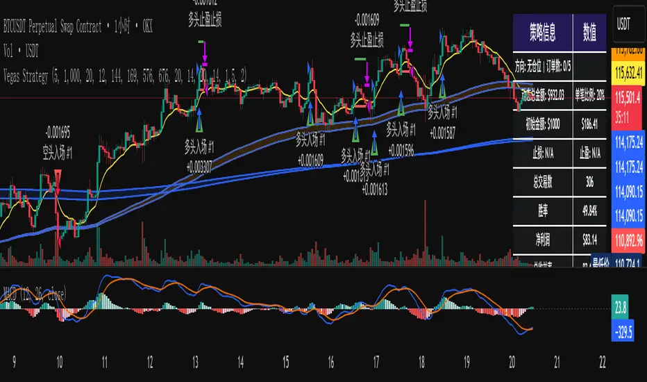
Bifurcation Zone - CAEBifurcation Zone — Cognitive Adversarial Engine (BZ-CAE)
Bifurcation Zone — CAE (BZ-CAE) is a next-generation divergence detection system enhanced by a Cognitive Adversarial Engine that evaluates both sides of every potential trade before presenting signals. Unlike traditional divergence indicators that show every price-oscillator disagreement regardless of context, BZ-CAE applies comprehensive market-state intelligence to identify only the divergences that occur in favorable conditions with genuine probability edges.
The system identifies structural bifurcation points — critical junctures where price and momentum disagree, signaling potential reversals or continuations — then validates these opportunities through five interconnected intelligence layers: Trend Conviction Scoring , Directional Momentum Alignment , Multi-Factor Exhaustion Modeling , Adversarial Validation , and Confidence Scoring . The result is a selective, context-aware signal system that filters noise and highlights high-probability setups.
This is not a "buy the arrow" indicator. It's a decision support framework that teaches you how to read market state, evaluate divergence quality, and make informed trading decisions based on quantified intelligence rather than hope.
What Sets BZ-CAE Apart: Technical Architecture
The Problem With Traditional Divergence Indicators
Most divergence indicators operate on a simple rule: if price makes a higher high and RSI makes a lower high, show a bearish signal. If price makes a lower low and RSI makes a higher low, show a bullish signal. This creates several critical problems:
Context Blindness : They show counter-trend signals in powerful trends that rarely reverse, leading to repeated losses as you fade momentum.
Signal Spam : Every minor price-oscillator disagreement generates an alert, overwhelming you with low-quality setups and creating analysis paralysis.
No Quality Ranking : All signals are treated identically. A marginal divergence in choppy conditions receives the same visual treatment as a high-conviction setup at a major exhaustion point.
Single-Sided Evaluation : They ask "Is this a good long?" without checking if the short case is overwhelmingly stronger, leading you into obvious bad trades.
Static Configuration : You manually choose RSI 14 or Stochastic 14 and hope it works, with no systematic way to validate if that's optimal for your instrument.
BZ-CAE's Solution: Cognitive Adversarial Intelligence
BZ-CAE solves these problems through an integrated five-layer intelligence architecture:
1. Trend Conviction Score (TCS) — 0 to 1 Scale
Most indicators check if ADX is above 25 to determine "trending" conditions. This binary approach misses nuance. TCS is a weighted composite metric:
Formula : 0.35 × normalize(ADX, 10, 35) + 0.35 × structural_strength + 0.30 × htf_alignment
Structural Strength : 10-bar SMA of consecutive directional bars. Captures persistence — are bulls or bears consistently winning?
HTF Alignment : Multi-timeframe EMA stacking (20/50/100/200). When all EMAs align in the same direction, you're in institutional trend territory.
Purpose : Quantifies how "locked in" the trend is. When TCS exceeds your threshold (default 0.80), the system knows to avoid counter-trend trades unless other factors override.
Interpretation :
TCS > 0.85: Very strong trend — counter-trading is extremely high risk
TCS 0.70-0.85: Strong trend — favor continuation, require exhaustion for reversals
TCS 0.50-0.70: Moderate trend — context matters, both directions viable
TCS < 0.50: Weak/choppy — reversals more viable, range-bound conditions
2. Directional Momentum Alignment (DMA) — ATR-Normalized
Formula : (EMA21 - EMA55) / ATR14
This isn't just "price above EMA" — it's a regime-aware momentum gauge. The same $100 price movement reads completely differently in high-volatility crypto versus low-volatility forex. By normalizing with ATR, DMA adapts its interpretation to current market conditions.
Purpose : Quantifies the directional "force" behind current price action. Positive = bullish push, negative = bearish push. Magnitude = strength.
Interpretation :
DMA > 0.7: Strong bullish momentum — bearish divergences risky
DMA 0.3 to 0.7: Moderate bullish bias
DMA -0.3 to 0.3: Balanced/choppy conditions
DMA -0.7 to -0.3: Moderate bearish bias
DMA < -0.7: Strong bearish momentum — bullish divergences risky
3. Multi-Factor Exhaustion Modeling — 0 to 1 Probability
Single-metric exhaustion detection (like "RSI > 80") misses complex market states. BZ-CAE aggregates five independent exhaustion signals:
Volume Spikes : Current volume versus 50-bar average
2.5x average: 0.25 weight
2.0x average: 0.15 weight
1.5x average: 0.10 weight
Divergence Present : The fact that a divergence exists contributes 0.30 weight — structural momentum disagreement is itself an exhaustion signal.
RSI Extremes : Captures oscillator climax zones
RSI > 80 or < 20: 0.25 weight
RSI > 75 or < 25: 0.15 weight
Pin Bar Detection : Identifies rejection candles (2:1 wick-to-body ratio, indicating failed breakout attempts): 0.15 weight
Extended Runs : Consecutive bars above/below EMA20 without pullback
30+ bars: 0.15 weight (market hasn't paused to consolidate)
Total exhaustion score is the sum of all applicable weights, capped at 1.0.
Purpose : Detects when strong trends become vulnerable to reversal. High exhaustion can override trend filters, allowing counter-trend trades at genuine turning points that basic indicators would miss.
Interpretation :
Exhaustion > 0.75: High probability of climax — yellow background shading alerts you visually
Exhaustion 0.50-0.75: Moderate overextension — watch for confirmation
Exhaustion < 0.50: Fresh move — trend can continue, counter-trend trades higher risk
4. Adversarial Validation — Game Theory Applied to Trading
This is BZ-CAE's signature innovation. Before approving any signal, the engine quantifies BOTH sides of the trade simultaneously:
For Bullish Divergences , it calculates:
Bull Case Score (0-1+) :
Distance below EMA20 (pullback quality): up to 0.25
Bullish EMA alignment (close > EMA20 > EMA50): 0.25
Oversold RSI (< 40): 0.25
Volume confirmation (> 1.2x average): 0.25
Bear Case Score (0-1+) :
Price below EMA50 (structural weakness): 0.30
Very oversold RSI (< 30, indicating knife-catching): 0.20
Differential = Bull Case - Bear Case
If differential < -0.10 (default threshold), the bear case is dominating — signal is BLOCKED or ANNOTATED.
For Bearish Divergences , the logic inverts (Bear Case vs Bull Case).
Purpose : Prevents trades where you're fighting obvious strength in the opposite direction. This is institutional-grade risk management — don't just evaluate your trade, evaluate the counter-trade simultaneously.
Why This Matters : You might see a bullish divergence at a local low, but if price is deeply below major support EMAs with strong bearish momentum, you're catching a falling knife. The adversarial check catches this and blocks the signal.
5. Confidence Scoring — 0 to 1 Quality Assessment
Every signal that passes initial filters receives a comprehensive quality score:
Formula :
0.30 × normalize(TCS) // Trend context
+ 0.25 × normalize(|DMA|) // Momentum magnitude
+ 0.20 × pullback_quality // Entry distance from EMA20
+ 0.15 × state_quality // ADX + alignment + structure
+ 0.10 × divergence_strength // Slope separation magnitude
+ adversarial_bonus (0-0.30) // Your side's advantage
Purpose : Ranks setup quality for filtering and position sizing decisions. You can set a minimum confidence threshold (default 0.35) to ensure only quality setups reach your chart.
Interpretation :
Confidence > 0.70: Premium setup — consider increased position size
Confidence 0.50-0.70: Good quality — standard size
Confidence 0.35-0.50: Acceptable — reduced size or skip if conservative
Confidence < 0.35: Marginal — blocked in Filtering mode, annotated in Advisory mode
CAE Operating Modes: Learning vs Enforcement
Off : Disables all CAE logic. Raw divergence pipeline only. Use for baseline comparison.
Advisory : Shows ALL signals regardless of CAE evaluation, but annotates signals that WOULD be blocked with specific warnings (e.g., "Bull: strong downtrend (TCS=0.87)" or "Adversarial bearish"). This is your learning mode — see CAE's decision logic in action without missing educational opportunities.
Filtering : Actively blocks low-quality signals. Only setups that pass all enabled gates (Trend Filter, Adversarial Validation, Confidence Gating) reach your chart. This is your live trading mode — trust the system to enforce discipline.
CAE Filter Gates: Three-Layer Protection
When CAE is enabled, signals must pass through three independent gates (each can be toggled on/off):
Gate 1: Strong Trend Filter
If TCS ≥ tcs_threshold (default 0.80)
And signal is counter-trend (bullish in downtrend or bearish in uptrend)
And exhaustion < exhaustion_required (default 0.50)
Then: BLOCK signal
Logic: Don't fade strong trends unless the move is clearly overextended
Gate 2: Adversarial Validation
Calculate both bull case and bear case scores
If opposing case dominates by more than adv_threshold (default 0.10)
Then: BLOCK signal
Logic: Avoid trades where you're fighting obvious strength in the opposite direction
Gate 3: Confidence Gating
Calculate composite confidence score (0-1)
If confidence < min_confidence (default 0.35)
Then: In Filtering mode, BLOCK signal; in Advisory mode, ANNOTATE with warning
Logic: Only take setups with minimum quality threshold
All three gates work together. A signal must pass ALL enabled gates to fire.
Visual Intelligence System
Bifurcation Zones (Supply/Demand Blocks)
When a divergence signal fires, BZ-CAE draws a semi-transparent box extending 15 bars forward from the signal pivot:
Demand Zones (Bullish) : Theme-colored box (cyan in Cyberpunk, blue in Professional, etc.) labeled "Demand" — marks where smart money likely placed buy orders as price diverged at the low.
Supply Zones (Bearish) : Theme-colored box (magenta in Cyberpunk, orange in Professional) labeled "Supply" — marks where smart money likely placed sell orders as price diverged at the high.
Theory : Divergences represent institutional disagreement with the crowd. The crowd pushed price to an extreme (new high or low), but momentum (oscillator) is waning, indicating smart money is taking the opposite side. These zones mark order placement areas that become future support/resistance.
Use Cases :
Exit targets: Take profit when price returns to opposite-side zone
Re-entry levels: If price returns to your entry zone, consider adding
Stop placement: Place stops just beyond your zone (below demand, above supply)
Auto-Cleanup : System keeps the last 20 zones to prevent chart clutter.
Adversarial Bar Coloring — Real-Time Market Debate Heatmap
Each bar is colored based on the Bull Case vs Bear Case differential:
Strong Bull Advantage (diff > 0.3): Full theme bull color (e.g., cyan)
Moderate Bull Advantage (diff > 0.1): 50% transparency bull
Neutral (diff -0.1 to 0.1): Gray/neutral theme
Moderate Bear Advantage (diff < -0.1): 50% transparency bear
Strong Bear Advantage (diff < -0.3): Full theme bear color (e.g., magenta)
This creates a real-time visual heatmap showing which side is "winning" the market debate. When bars flip from cyan to magenta (or vice versa), you're witnessing a shift in adversarial advantage — a leading indicator of potential momentum changes.
Exhaustion Shading
When exhaustion score exceeds 0.75, the chart background displays a semi-transparent yellow highlight. This immediate visual warning alerts you that the current move is at high risk of reversal, even if trend indicators remain strong.
Visual Themes — Six Aesthetic Options
Cyberpunk : Cyan/Magenta/Yellow — High contrast, neon aesthetic, excellent for dark-themed trading environments
Professional : Blue/Orange/Green — Corporate color palette, suitable for presentations and professional documentation
Ocean : Teal/Red/Cyan — Aquatic palette, calming for extended monitoring sessions
Fire : Orange/Red/Coral — Warm aggressive colors, high energy
Matrix : Green/Red/Lime — Code aesthetic, homage to classic hacker visuals
Monochrome : White/Gray — Minimal distraction, maximum focus on price action
All visual elements (signal markers, zones, bar colors, dashboard) adapt to your selected theme.
Divergence Engine — Core Detection System
What Are Divergences?
Divergences occur when price action and momentum indicators disagree, creating structural tension that often resolves in a change of direction:
Regular Divergence (Reversal Signal) :
Bearish Regular : Price makes higher high, oscillator makes lower high → Potential trend reversal down
Bullish Regular : Price makes lower low, oscillator makes higher low → Potential trend reversal up
Hidden Divergence (Continuation Signal) :
Bearish Hidden : Price makes lower high, oscillator makes higher high → Downtrend continuation
Bullish Hidden : Price makes higher low, oscillator makes lower low → Uptrend continuation
Both types can be enabled/disabled independently in settings.
Pivot Detection Methods
BZ-CAE uses symmetric pivot detection with separate lookback and lookforward periods (default 5/5):
Pivot High : Bar where high > all highs within lookback range AND high > all highs within lookforward range
Pivot Low : Bar where low < all lows within lookback range AND low < all lows within lookforward range
This ensures structural validity — the pivot must be a clear local extreme, not just a minor wiggle.
Divergence Validation Requirements
For a divergence to be confirmed, it must satisfy:
Slope Disagreement : Price slope and oscillator slope must move in opposite directions (for regular divs) or same direction with inverted highs/lows (for hidden divs)
Minimum Slope Change : |osc_slope| > min_slope_change / 100 (default 1.0) — filters weak, marginal divergences
Maximum Lookback Range : Pivots must be within max_lookback bars (default 60) — prevents ancient, irrelevant divergences
ATR-Normalized Strength : Divergence strength = min(|price_slope| × |osc_slope| × 10, 1.0) — quantifies the magnitude of disagreement in volatility context
Regular divergences receive 1.0× weight; hidden divergences receive 0.8× weight (slightly less reliable historically).
Oscillator Options — Five Professional Indicators
RSI (Relative Strength Index) : Classic overbought/oversold momentum indicator. Best for: General purpose divergence detection across all instruments.
Stochastic : Range-bound %K momentum comparing close to high-low range. Best for: Mean reversion strategies and range-bound markets.
CCI (Commodity Channel Index) : Measures deviation from statistical mean, auto-normalized to 0-100 scale. Best for: Cyclical instruments and commodities.
MFI (Money Flow Index) : Volume-weighted RSI incorporating money flow. Best for: Volume-driven markets like stocks and crypto.
Williams %R : Inverse stochastic looking back over period, auto-adjusted to 0-100. Best for: Reversal detection at extremes.
Each oscillator has adjustable length (2-200, default 14) and smoothing (1-20, default 1). You also set overbought (50-100, default 70) and oversold (0-50, default 30) thresholds.
Signal Timing Modes — Understanding Repainting
BZ-CAE offers two timing policies with complete transparency about repainting behavior:
Realtime (1-bar, peak-anchored)
How It Works :
Detects peaks 1 bar ago using pattern: high > high AND high > high
Signal prints on the NEXT bar after peak detection (bar_index)
Visual marker anchors to the actual PEAK bar (bar_index - 1, offset -1)
Signal locks in when bar CONFIRMS (closes)
Repainting Behavior :
On the FORMING bar (before close), the peak condition may change as new prices arrive
Once bar CLOSES (barstate.isconfirmed), signal is locked permanently
This is preview/early warning behavior by design
Best For :
Active monitoring and immediate alerts
Learning the system (seeing signals develop in real-time)
Responsive entry if you're watching the chart live
Confirmed (lookforward)
How It Works :
Uses Pine Script's built-in ta.pivothigh() and ta.pivotlow() functions
Requires full pivot validation period (lookback + lookforward bars)
Signal prints pivot_lookforward bars after the actual peak (default 5-bar delay)
Visual marker anchors to the actual peak bar (offset -pivot_lookforward)
No Repainting Behavior
Best For :
Backtesting and historical analysis
Conservative entries requiring full confirmation
Automated trading systems
Swing trading with larger timeframes
Tradeoff :
Delayed entry by pivot_lookforward bars (typically 5 bars)
On a 5-minute chart, this is a 25-minute delay
On a 4-hour chart, this is a 20-hour delay
Recommendation : Use Confirmed for backtesting to verify system performance honestly. Use Realtime for live monitoring only if you're actively watching the chart and understand pre-confirmation repainting behavior.
Signal Spacing System — Anti-Spam Architecture
Even after CAE filtering, raw divergences can cluster. The spacing system enforces separation:
Three Independent Filters
1. Min Bars Between ANY Signals (default 12):
Prevents rapid-fire clustering across both directions
If last signal (bull or bear) was within N bars, block new signal
Ensures breathing room between all setups
2. Min Bars Between SAME-SIDE Signals (default 24, optional enforcement):
Prevents bull-bull or bear-bear spam
Separate tracking for bullish and bearish signal timelines
Toggle enforcement on/off
3. Min ATR Distance From Last Signal (default 0, optional):
Requires price to move N × ATR from last signal location
Ensures meaningful price movement between setups
0 = disabled, 0.5-2.0 = typical range for enabled
All three filters work independently. A signal must pass ALL enabled filters to proceed.
Practical Guidance :
Scalping (1-5m) : Any 6-10, Same-side 12-20, ATR 0-0.5
Day Trading (15m-1H) : Any 12, Same-side 24, ATR 0-1.0
Swing Trading (4H-D) : Any 20-30, Same-side 40-60, ATR 1.0-2.0
Dashboard — Real-Time Control Center
The dashboard (toggleable, four corner positions, three sizes) provides comprehensive system intelligence:
Oscillator Section
Current oscillator type and value
State: OVERBOUGHT / OVERSOLD / NEUTRAL (color-coded)
Length parameter
Cognitive Engine Section
TCS (Trend Conviction Score) :
Current value with emoji state indicator
🔥 = Strong trend (>0.75)
📊 = Moderate trend (0.50-0.75)
〰️ = Weak/choppy (<0.50)
Color: Red if above threshold (trend filter active), yellow if moderate, green if weak
DMA (Directional Momentum Alignment) :
Current value with emoji direction indicator
🐂 = Bullish momentum (>0.5)
⚖️ = Balanced (-0.5 to 0.5)
🐻 = Bearish momentum (<-0.5)
Color: Green if bullish, red if bearish
Exhaustion :
Current value with emoji warning indicator
⚠️ = High exhaustion (>0.75)
🟡 = Moderate (0.50-0.75)
✓ = Low (<0.50)
Color: Red if high, yellow if moderate, green if low
Pullback :
Quality of current distance from EMA20
Values >0.6 are ideal entry zones (not too close, not too far)
Bull Case / Bear Case (if Adversarial enabled):
Current scores for both sides of the market debate
Differential with emoji indicator:
📈 = Bull advantage (>0.2)
➡️ = Balanced (-0.2 to 0.2)
📉 = Bear advantage (<-0.2)
Last Signal Metrics Section (New Feature)
When a signal fires, this section captures and displays:
Signal type (BULL or BEAR)
Bars elapsed since signal
Confidence % at time of signal
TCS value at signal time
DMA value at signal time
Purpose : Provides a historical reference for learning. You can see what the market state looked like when the last signal fired, helping you correlate outcomes with conditions.
Statistics Section
Total Signals : Lifetime count across session
Blocked Signals : Count and percentage (filter effectiveness metric)
Bull Signals : Total bullish divergences
Bear Signals : Total bearish divergences
Purpose : System health monitoring. If blocked % is very high (>60%), filters may be too strict. If very low (<10%), filters may be too loose.
Advisory Annotations
When CAE Mode = Advisory, this section displays warnings for signals that would be blocked in Filtering mode:
Examples:
"Bull spacing: wait 8 bars"
"Bear: strong uptrend (TCS=0.87)"
"Adversarial bearish"
"Low confidence 32%"
Multiple warnings can stack, separated by " | ". This teaches you CAE's decision logic transparently.
How to Use BZ-CAE — Complete Workflow
Phase 1: Initial Setup (First Session)
Apply BZ-CAE to your chart
Select your preferred Visual Theme (Cyberpunk recommended for visibility)
Set Signal Timing to "Confirmed (lookforward)" for learning
Choose your Oscillator Type (RSI recommended for general use, length 14)
Set Overbought/Oversold to 70/30 (standard)
Enable both Regular Divergence and Hidden Divergence
Set Pivot Lookback/Lookforward to 5/5 (balanced structure)
Enable CAE Intelligence
Set CAE Mode to "Advisory" (learning mode)
Enable all three CAE filters: Strong Trend Filter , Adversarial Validation , Confidence Gating
Enable Show Dashboard , position Top Right, size Normal
Enable Draw Bifurcation Zones and Adversarial Bar Coloring
Phase 2: Learning Period (Weeks 1-2)
Goal : Understand how CAE evaluates market state and filters signals.
Activities :
Watch the dashboard during signals :
Note TCS values when counter-trend signals fail — this teaches you the trend strength threshold for your instrument
Observe exhaustion patterns at actual turning points — learn when overextension truly matters
Study adversarial differential at signal times — see when opposing cases dominate
Review blocked signals (orange X-crosses):
In Advisory mode, you see everything — signals that would pass AND signals that would be blocked
Check the advisory annotations to understand why CAE would block
Track outcomes: Were the blocks correct? Did those signals fail?
Use Last Signal Metrics :
After each signal, check the dashboard capture of confidence, TCS, and DMA
Journal these values alongside trade outcomes
Identify patterns: Do confidence >0.70 signals work better? Does your instrument respect TCS >0.85?
Understand your instrument's "personality" :
Trending instruments (indices, major forex) may need TCS threshold 0.85-0.90
Choppy instruments (low-cap stocks, exotic pairs) may work best with TCS 0.70-0.75
High-volatility instruments (crypto) may need wider spacing
Low-volatility instruments may need tighter spacing
Phase 3: Calibration (Weeks 3-4)
Goal : Optimize settings for your specific instrument, timeframe, and style.
Calibration Checklist :
Min Confidence Threshold :
Review confidence distribution in your signal journal
Identify the confidence level below which signals consistently fail
Set min_confidence slightly above that level
Day trading : 0.35-0.45
Swing trading : 0.40-0.55
Scalping : 0.30-0.40
TCS Threshold :
Find the TCS level where counter-trend signals consistently get stopped out
Set tcs_threshold at or slightly below that level
Trending instruments : 0.85-0.90
Mixed instruments : 0.80-0.85
Choppy instruments : 0.75-0.80
Exhaustion Override Level :
Identify exhaustion readings that marked genuine reversals
Set exhaustion_required just below the average
Typical range : 0.45-0.55
Adversarial Threshold :
Default 0.10 works for most instruments
If you find CAE is too conservative (blocking good trades), raise to 0.15-0.20
If signals are still getting caught in opposing momentum, lower to 0.07-0.09
Spacing Parameters :
Count bars between quality signals in your journal
Set min bars ANY to ~60% of that average
Set min bars SAME-SIDE to ~120% of that average
Scalping : Any 6-10, Same 12-20
Day trading : Any 12, Same 24
Swing : Any 20-30, Same 40-60
Oscillator Selection :
Try different oscillators for 1-2 weeks each
Track win rate and average winner/loser by oscillator type
RSI : Best for general use, clear OB/OS
Stochastic : Best for range-bound, mean reversion
MFI : Best for volume-driven markets
CCI : Best for cyclical instruments
Williams %R : Best for reversal detection
Phase 4: Live Deployment
Goal : Disciplined execution with proven, calibrated system.
Settings Changes :
Switch CAE Mode from Advisory to Filtering
System now actively blocks low-quality signals
Only setups passing all gates reach your chart
Keep Signal Timing on Confirmed for conservative entries
OR switch to Realtime if you're actively monitoring and want faster entries (accept pre-confirmation repaint risk)
Use your calibrated thresholds from Phase 3
Enable high-confidence alerts: "⭐ High Confidence Bullish/Bearish" (>0.70)
Trading Discipline Rules :
Respect Blocked Signals :
If CAE blocks a trade you wanted to take, TRUST THE SYSTEM
Don't manually override — if you consistently disagree, return to Phase 2/3 calibration
The block exists because market state failed intelligence checks
Confidence-Based Position Sizing :
Confidence >0.70: Standard or increased size (e.g., 1.5-2.0% risk)
Confidence 0.50-0.70: Standard size (e.g., 1.0% risk)
Confidence 0.35-0.50: Reduced size (e.g., 0.5% risk) or skip if conservative
TCS-Based Management :
High TCS + counter-trend signal: Use tight stops, quick exits (you're fading momentum)
Low TCS + reversal signal: Use wider stops, trail aggressively (genuine reversal potential)
Exhaustion Awareness :
Exhaustion >0.75 (yellow shading): Market is overextended, reversal risk is elevated — consider early exit or tighter trailing stops even on winning trades
Exhaustion <0.30: Continuation bias — hold for larger move, wide trailing stops
Adversarial Context :
Strong differential against you (e.g., bullish signal with bear diff <-0.2): Use very tight stops, consider skipping
Strong differential with you (e.g., bullish signal with bull diff >0.2): Trail aggressively, this is your tailwind
Practical Settings by Timeframe & Style
Scalping (1-5 Minute Charts)
Objective : High frequency, tight stops, quick reversals in fast-moving markets.
Oscillator :
Type: RSI or Stochastic (fast response to quick moves)
Length: 9-11 (more responsive than standard 14)
Smoothing: 1 (no lag)
OB/OS: 65/35 (looser thresholds ensure frequent crossings in fast conditions)
Divergence :
Pivot Lookback/Lookforward: 3/3 (tight structure, catch small swings)
Max Lookback: 40-50 bars (recent structure only)
Min Slope Change: 0.8-1.0 (don't be overly strict)
CAE :
Mode: Advisory first (learn), then Filtering
Min Confidence: 0.30-0.35 (lower bar for speed, accept more signals)
TCS Threshold: 0.70-0.75 (allow more counter-trend opportunities)
Exhaustion Required: 0.45-0.50 (moderate override)
Strong Trend Filter: ON (still respect major intraday trends)
Adversarial: ON (critical for scalping protection — catches bad entries quickly)
Spacing :
Min Bars ANY: 6-10 (fast pace, many setups)
Min Bars SAME-SIDE: 12-20 (prevent clustering)
Min ATR Distance: 0 or 0.5 (loose)
Timing : Realtime (speed over precision, but understand repaint risk)
Visuals :
Signal Size: Tiny (chart clarity in busy conditions)
Show Zones: Optional (can clutter on low timeframes)
Bar Coloring: ON (helps read momentum shifts quickly)
Dashboard: Small size (corner reference, not main focus)
Key Consideration : Scalping generates noise. Even with CAE, expect lower win rate (45-55%) but aim for favorable R:R (2:1 or better). Size conservatively.
Day Trading (15-Minute to 1-Hour Charts)
Objective : Balance quality and frequency. Standard divergence trading approach.
Oscillator :
Type: RSI or MFI (proven reliability, volume confirmation with MFI)
Length: 14 (industry standard, well-studied)
Smoothing: 1-2
OB/OS: 70/30 (classic levels)
Divergence :
Pivot Lookback/Lookforward: 5/5 (balanced structure)
Max Lookback: 60 bars
Min Slope Change: 1.0 (standard strictness)
CAE :
Mode: Filtering (enforce discipline from the start after brief Advisory learning)
Min Confidence: 0.35-0.45 (quality filter without being too restrictive)
TCS Threshold: 0.80-0.85 (respect strong trends)
Exhaustion Required: 0.50 (balanced override threshold)
Strong Trend Filter: ON
Adversarial: ON
Confidence Gating: ON (all three filters active)
Spacing :
Min Bars ANY: 12 (breathing room between all setups)
Min Bars SAME-SIDE: 24 (prevent bull/bear clusters)
Min ATR Distance: 0-1.0 (optional refinement, typically 0.5-1.0)
Timing : Confirmed (1-bar delay for reliability, no repainting)
Visuals :
Signal Size: Tiny or Small
Show Zones: ON (useful reference for exits/re-entries)
Bar Coloring: ON (context awareness)
Dashboard: Normal size (full visibility)
Key Consideration : This is the "sweet spot" timeframe for BZ-CAE. Market structure is clear, CAE has sufficient data, and signal frequency is manageable. Expect 55-65% win rate with proper execution.
Swing Trading (4-Hour to Daily Charts)
Objective : Quality over quantity. High conviction only. Larger stops and targets.
Oscillator :
Type: RSI or CCI (robust on higher timeframes, smooth longer waves)
Length: 14-21 (capture larger momentum swings)
Smoothing: 1-3
OB/OS: 70/30 or 75/25 (strict extremes)
Divergence :
Pivot Lookback/Lookforward: 5/5 or 7/7 (structural purity, major swings only)
Max Lookback: 80-100 bars (broader historical context)
Min Slope Change: 1.2-1.5 (require strong, undeniable divergence)
CAE :
Mode: Filtering (strict enforcement, premium setups only)
Min Confidence: 0.40-0.55 (high bar for entry)
TCS Threshold: 0.85-0.95 (very strong trend protection — don't fade established HTF trends)
Exhaustion Required: 0.50-0.60 (higher bar for override — only extreme exhaustion justifies counter-trend)
Strong Trend Filter: ON (critical on HTF)
Adversarial: ON (avoid obvious bad trades)
Confidence Gating: ON (quality gate essential)
Spacing :
Min Bars ANY: 20-30 (substantial separation)
Min Bars SAME-SIDE: 40-60 (significant breathing room)
Min ATR Distance: 1.0-2.0 (require meaningful price movement)
Timing : Confirmed (purity over speed, zero repaint for swing accuracy)
Visuals :
Signal Size: Small or Normal (clear markers on zoomed-out view)
Show Zones: ON (important HTF levels)
Bar Coloring: ON (long-term trend awareness)
Dashboard: Normal or Large (comprehensive analysis)
Key Consideration : Swing signals are rare but powerful. Expect 2-5 signals per month per instrument. Win rate should be 60-70%+ due to stringent filtering. Position size can be larger given confidence.
Dashboard Interpretation Reference
TCS (Trend Conviction Score) States
0.00-0.50: Weak/Choppy
Emoji: 〰️
Color: Green/cyan
Meaning: No established trend. Range-bound or consolidating. Both reversal and continuation signals viable.
Action: Reversals (regular divs) are safer. Use wider profit targets (market has room to move). Consider mean reversion strategies.
0.50-0.75: Moderate Trend
Emoji: 📊
Color: Yellow/neutral
Meaning: Developing trend but not locked in. Context matters significantly.
Action: Check DMA and exhaustion. If DMA confirms trend and exhaustion is low, favor continuation (hidden divs). If exhaustion is high, reversals are viable.
0.75-0.85: Strong Trend
Emoji: 🔥
Color: Orange/warning
Meaning: Well-established trend with persistence. Counter-trend is high risk.
Action: Require exhaustion >0.50 for counter-trend entries. Favor continuation signals. Use tight stops on counter-trend attempts.
0.85-1.00: Very Strong Trend
Emoji: 🔥🔥
Color: Red/danger (if counter-trading)
Meaning: Locked-in institutional trend. Extremely high risk to fade.
Action: Avoid counter-trend unless exhaustion >0.75 (yellow shading). Focus exclusively on continuation opportunities. Momentum is king here.
DMA (Directional Momentum Alignment) Zones
-2.0 to -1.0: Strong Bearish Momentum
Emoji: 🐻🐻
Color: Dark red
Meaning: Powerful downside force. Sellers are in control.
Action: Bullish divergences are counter-momentum (high risk). Bearish divergences are with-momentum (lower risk). Size down on longs.
-0.5 to 0.5: Neutral/Balanced
Emoji: ⚖️
Color: Gray/neutral
Meaning: No strong directional bias. Choppy or consolidating.
Action: Both directions have similar probability. Focus on confidence score and adversarial differential for edge.
1.0 to 2.0: Strong Bullish Momentum
Emoji: 🐂🐂
Color: Bright green/cyan
Meaning: Powerful upside force. Buyers are in control.
Action: Bearish divergences are counter-momentum (high risk). Bullish divergences are with-momentum (lower risk). Size down on shorts.
Exhaustion States
0.00-0.50: Fresh Move
Emoji: ✓
Color: Green
Meaning: Trend is healthy, not overextended. Room to run.
Action: Counter-trend trades are premature. Favor continuation. Hold winners for larger moves. Avoid early exits.
0.50-0.75: Mature Move
Emoji: 🟡
Color: Yellow
Meaning: Move is aging. Watch for signs of climax.
Action: Tighten trailing stops on winning trades. Be ready for reversals. Don't add to positions aggressively.
0.75-0.85: High Exhaustion
Emoji: ⚠️
Color: Orange
Background: Yellow shading appears
Meaning: Move is overextended. Reversal risk elevated significantly.
Action: Counter-trend reversals are higher probability. Consider early exits on with-trend positions. Size up on reversal divergences (if CAE allows).
0.85-1.00: Critical Exhaustion
Emoji: ⚠️⚠️
Color: Red
Background: Yellow shading intensifies
Meaning: Climax conditions. Reversal imminent or underway.
Action: Aggressive reversal trades justified. Exit all with-trend positions. This is where major turns occur.
Confidence Score Tiers
0.00-0.30: Low Quality
Color: Red
Status: Blocked in Filtering mode
Action: Skip entirely. Setup lacks fundamental quality across multiple factors.
0.30-0.50: Moderate Quality
Color: Yellow/orange
Status: Marginal — passes in Filtering only if >min_confidence
Action: Reduced position size (0.5-0.75% risk). Tight stops. Conservative profit targets. Skip if you're selective.
0.50-0.70: High Quality
Color: Green/cyan
Status: Good setup across most quality factors
Action: Standard position size (1.0-1.5% risk). Normal stops and targets. This is your bread-and-butter trade.
0.70-1.00: Premium Quality
Color: Bright green/gold
Status: Exceptional setup — all factors aligned
Visual: Double confidence ring appears
Action: Consider increased position size (1.5-2.0% risk, maximum). Wider stops. Larger targets. High probability of success. These are rare — capitalize when they appear.
Adversarial Differential Interpretation
Bull Differential > 0.3 :
Visual: Strong cyan/green bar colors
Meaning: Bull case strongly dominates. Buyers have clear advantage.
Action: Bullish divergences favored (with-advantage). Bearish divergences face headwind (reduce size or skip). Momentum is bullish.
Bull Differential 0.1 to 0.3 :
Visual: Moderate cyan/green transparency
Meaning: Moderate bull advantage. Buyers have edge but not overwhelming.
Action: Both directions viable. Slight bias toward longs.
Differential -0.1 to 0.1 :
Visual: Gray/neutral bars
Meaning: Balanced debate. No clear advantage either side.
Action: Rely on other factors (confidence, TCS, exhaustion) for direction. Adversarial is neutral.
Bear Differential -0.3 to -0.1 :
Visual: Moderate red/magenta transparency
Meaning: Moderate bear advantage. Sellers have edge but not overwhelming.
Action: Both directions viable. Slight bias toward shorts.
Bear Differential < -0.3 :
Visual: Strong red/magenta bar colors
Meaning: Bear case strongly dominates. Sellers have clear advantage.
Action: Bearish divergences favored (with-advantage). Bullish divergences face headwind (reduce size or skip). Momentum is bearish.
Last Signal Metrics — Post-Trade Analysis
After a signal fires, dashboard captures:
Type : BULL or BEAR
Bars Ago : How long since signal (updates every bar)
Confidence : What was the quality score at signal time
TCS : What was trend conviction at signal time
DMA : What was momentum alignment at signal time
Use Case : Post-trade journaling and learning.
Example: "BULL signal 12 bars ago. Confidence: 68%, TCS: 0.42, DMA: -0.85"
Analysis : This was a bullish reversal (regular div) with good confidence, weak trend (TCS), but strong bearish momentum (DMA). The bet was that momentum would reverse — a counter-momentum play requiring exhaustion confirmation. Check if exhaustion was high at that time to justify the entry.
Track patterns:
Do your best trades have confidence >0.65?
Do low-TCS signals (<0.50) work better for you?
Are you more successful with-momentum (DMA aligned with signal) or counter-momentum?
Troubleshooting Guide
Problem: No Signals Appearing
Symptoms : Chart loads, dashboard shows metrics, but no divergence signals fire.
Diagnosis Checklist :
Check dashboard oscillator value : Is it crossing OB/OS levels (70/30)? If oscillator stays in 40-60 range constantly, it can't reach extremes needed for divergence detection.
Are pivots forming? : Look for local swing highs/lows on your chart. If price is in tight consolidation, pivots may not meet lookback/lookforward requirements.
Is spacing too tight? : Check "Last Signal" metrics — how many bars since last signal? If <12 and your min_bars_ANY is 12, spacing filter is blocking.
Is CAE blocking everything? : Check dashboard Statistics section — what's the blocked signal count? High blocks indicate overly strict filters.
Solutions :
Loosen OB/OS Temporarily :
Try 65/35 to verify divergence detection works
If signals appear, the issue was threshold strictness
Gradually tighten back to 67/33, then 70/30 as appropriate
Lower Min Confidence :
Try 0.25-0.30 (diagnostic level)
If signals appear, filter was too strict
Raise gradually to find sweet spot (0.35-0.45 typical)
Disable Strong Trend Filter Temporarily :
Turn off in CAE settings
If signals appear, TCS threshold was blocking everything
Re-enable and lower TCS_threshold to 0.70-0.75
Reduce Min Slope Change :
Try 0.7-0.8 (from default 1.0)
Allows weaker divergences through
Helpful on low-volatility instruments
Widen Spacing :
Set min_bars_ANY to 6-8
Set min_bars_SAME_SIDE to 12-16
Reduces time between allowed signals
Check Timing Mode :
If using Confirmed, remember there's a pivot_lookforward delay (5+ bars)
Switch to Realtime temporarily to verify system is working
Realtime has no delay but repaints
Verify Oscillator Settings :
Length 14 is standard but might not fit all instruments
Try length 9-11 for faster response
Try length 18-21 for slower, smoother response
Problem: Too Many Signals (Signal Spam)
Symptoms : Dashboard shows 50+ signals in Statistics, confidence scores mostly <0.40, signals clustering close together.
Solutions :
Raise Min Confidence :
Try 0.40-0.50 (quality filter)
Blocks bottom-tier setups
Targets top 50-60% of divergences only
Tighten OB/OS :
Use 70/30 or 75/25
Requires more extreme oscillator readings
Reduces false divergences in mid-range
Increase Min Slope Change :
Try 1.2-1.5 (from default 1.0)
Requires stronger, more obvious divergences
Filters marginal slope disagreements
Raise TCS Threshold :
Try 0.85-0.90 (from default 0.80)
Stricter trend filter blocks more counter-trend attempts
Favors only strongest trend alignment
Enable ALL CAE Gates :
Turn on Trend Filter + Adversarial + Confidence
Triple-layer protection
Blocks aggressively — expect 20-40% reduction in signals
Widen Spacing :
min_bars_ANY: 15-20 (from 12)
min_bars_SAME_SIDE: 30-40 (from 24)
Creates substantial breathing room
Switch to Confirmed Timing :
Removes realtime preview noise
Ensures full pivot validation
5-bar delay filters many false starts
Problem: Signals in Strong Trends Get Stopped Out
Symptoms : You take a bullish divergence in a downtrend (or bearish in uptrend), and it immediately fails. Dashboard showed high TCS at the time.
Analysis : This is INTENDED behavior — CAE is protecting you from low-probability counter-trend trades.
Understanding :
Check Last Signal Metrics in dashboard — what was TCS when signal fired?
If TCS was >0.85 and signal was counter-trend, CAE correctly identified it as high risk
Strong trends rarely reverse cleanly without major exhaustion
Your losses here are the system working as designed (blocking bad odds)
If You Want to Override (Not Recommended) :
Lower TCS_threshold to 0.70-0.75 (allows more counter-trend)
Lower exhaustion_required to 0.40 (easier override)
Disable Strong Trend Filter entirely (very risky)
Better Approach :
TRUST THE FILTER — it's preventing costly mistakes
Wait for exhaustion >0.75 (yellow shading) before counter-trending strong TCS
Focus on continuation signals (hidden divs) in high-TCS environments
Use Advisory mode to see what CAE is blocking and learn from outcomes
Problem: Adversarial Blocking Seems Wrong
Symptoms : You see a divergence that "looks good" visually, but CAE blocks with "Adversarial bearish/bullish" warning.
Diagnosis :
Check dashboard Bull Case and Bear Case scores at that moment
Look at Differential value
Check adversarial bar colors — was there strong coloring against your intended direction?
Understanding :
Adversarial catches "obvious" opposing momentum that's easy to miss
Example: Bullish divergence at a local low, BUT price is deeply below EMA50, bearish momentum is strong, and RSI shows knife-catching conditions
Bull Case might be 0.20 while Bear Case is 0.55
Differential = -0.35, far beyond threshold
Block is CORRECT — you'd be fighting overwhelming opposing flow
If You Disagree Consistently
Review blocked signals on chart — scroll back and check outcomes
Did those blocked signals actually work, or did they fail as adversarial predicted?
Raise adv_threshold to 0.15-0.20 (more permissive, allows closer battles)
Disable Adversarial Validation temporarily (diagnostic) to isolate its effect
Use Advisory mode to learn adversarial patterns over 50-100 signals
Remember : Adversarial is conservative BY DESIGN. It prevents "obvious" bad trades where you're fighting strong strength the other way.
Problem: Dashboard Not Showing or Incomplete
Solutions :
Toggle "Show Dashboard" to ON in settings
Try different dashboard sizes (Small/Normal/Large)
Try different positions (Top Left/Right, Bottom Left/Right) — might be off-screen
Some sections require CAE Enable = ON (Cognitive Engine section won't appear if CAE is disabled)
Statistics section requires at least 1 lifetime signal to populate
Check that visual theme is set (dashboard colors adapt to theme)
Problem: Performance Lag, Chart Freezing
Symptoms : Chart loading is slow, indicator calculations cause delays, pinch-to-zoom lags.
Diagnosis : Visual features are computationally expensive, especially adversarial bar coloring (recalculates every bar).
Solutions (In Order of Impact) :
Disable Adversarial Bar Coloring (MOST EXPENSIVE):
Turn OFF "Adversarial Bar Coloring" in settings
This is the single biggest performance drain
Immediate improvement
Reduce Vertical Lines :
Lower "Keep last N vertical lines" to 20-30
Or set to 0 to disable entirely
Moderate improvement
Disable Bifurcation Zones :
Turn OFF "Draw Bifurcation Zones"
Reduces box drawing calculations
Moderate improvement
Set Dashboard Size to Small :
Smaller dashboard = fewer cells = less rendering
Minor improvement
Use Shorter Max Lookback :
Reduce max_lookback to 40-50 (from 60+)
Fewer bars to scan for divergences
Minor improvement
Disable Exhaustion Shading :
Turn OFF "Show Market State"
Removes background coloring calculations
Minor improvement
Extreme Performance Mode :
Disable ALL visual enhancements
Keep only triangle markers
Dashboard Small or OFF
Use Minimal theme if available
Problem: Realtime Signals Repainting
Symptoms : You see a signal appear, but on next bar it disappears or moves.
Explanation :
Realtime mode detects peaks 1 bar ago: high > high AND high > high
On the FORMING bar (before close), this condition can change as new prices arrive
Example: At 10:05, high (10:04 bar) was 100, current high is 99 → peak detected
At 10:05:30, new high of 101 arrives → peak condition breaks → signal disappears
At 10:06 (bar close), final high is 101 → no peak at 10:04 anymore → signal gone permanently
This is expected behavior for realtime responsiveness. You get preview/early warning, but it's not locked until bar confirms.
Solutions :
Use Confirmed Timing :
Switch to "Confirmed (lookforward)" mode
ZERO repainting — pivot must be fully validated
5-bar delay (pivot_lookforward)
What you see in history is exactly what would have appeared live
Accept Realtime Repaint as Tradeoff :
Keep Realtime mode for speed and alerts
Understand that pre-confirmation signals may vanish
Only trade signals that CONFIRM at bar close (check barstate.isconfirmed)
Use for live monitoring, NOT for backtesting
Trade Only After Confirmation :
In Realtime mode, wait 1 full bar after signal appears before entering
If signal survives that bar close, it's locked
This adds 1-bar delay but removes repaint risk
Recommendation : Use Confirmed for backtesting and conservative trading. Use Realtime only for active monitoring with full understanding of preview behavior.
Risk Management Integration
BZ-CAE is a signal generation system, not a complete trading strategy. You must integrate proper risk management:
Position Sizing by Confidence
Confidence 0.70-1.00 (Premium) :
Risk: 1.5-2.0% of account (MAXIMUM)
Reasoning: High-quality setup across all factors
Still cap at 2% — even premium setups can fail
Confidence 0.50-0.70 (High Quality) :
Risk: 1.0-1.5% of account
Reasoning: Standard good setup
Your bread-and-butter risk level
Confidence 0.35-0.50 (Moderate Quality) :
Risk: 0.5-1.0% of account
Reasoning: Marginal setup, passes minimum threshold
Reduce size or skip if you're selective
Confidence <0.35 (Low Quality) :
Risk: 0% (blocked in Filtering mode)
Reasoning: Insufficient quality factors
System protects you by not showing these
Stop Placement Strategies
For Reversal Signals (Regular Divergences) :
Place stop beyond the divergence pivot plus buffer
Bullish : Stop below the divergence low - 1.0-1.5 × ATR
Bearish : Stop above the divergence high + 1.0-1.5 × ATR
Reasoning: If price breaks the pivot, divergence structure is invalidated
For Continuation Signals (Hidden Divergences) :
Place stop beyond recent swing in opposite direction
Bullish continuation : Stop below recent swing low (not the divergence pivot itself)
Bearish continuation : Stop above recent swing high
Reasoning: You're trading with trend, allow more breathing room
ATR-Based Stops :
1.5-2.0 × ATR is standard
Scale by timeframe:
Scalping (1-5m): 1.0-1.5 × ATR (tight)
Day trading (15m-1H): 1.5-2.0 × ATR (balanced)
Swing (4H-D): 2.0-3.0 × ATR (wide)
Never Use Fixed Dollar/Pip Stops :
Markets have different volatility
50-pip stop on EUR/USD ≠ 50-pip stop on GBP/JPY
Always normalize by ATR or pivot structure
Profit Targets and Scaling
Primary Target :
2-3 × ATR from entry (minimum 2:1 reward-risk)
Example : Entry at 100, ATR = 2, stop at 97 (1.5 × ATR) → target at 106 (3 × ATR) = 2:1 R:R
Scaling Out Strategy :
Take 50% off at 1.5 × ATR (secure partial profit)
Move stop to breakeven
Trail remaining 50% with 1.0 × ATR trailing stop
Let winners run if trend persists
Targets by Confidence :
High Confidence (>0.70) : Aggressive targets (3-4 × ATR), trail wider (1.5 × ATR)
Standard Confidence (0.50-0.70) : Normal targets (2-3 × ATR), standard trail (1.0 × ATR)
Low Confidence (0.35-0.50) : Conservative targets (1.5-2 × ATR), tight trail (0.75 × ATR)
Use Bifurcation Zones :
If opposite-side zone is visible on chart (from previous signal), use it as target
Example : Bullish signal at 100, prior supply zone at 110 → use 110 as target
Zones mark institutional resistance/support
Exhaustion-Based Exits :
If you're in a trade and exhaustion >0.75 develops (yellow shading), consider early exit
Market is overextended — reversal risk is high
Take profit even if target not reached
Trade Management by TCS
High TCS + Counter-Trend Trade (Risky) :
Use very tight stops (1.0-1.5 × ATR)
Conservative targets (1.5-2 × ATR)
Quick exit if trade doesn't work immediately
You're fading momentum — respect it
Low TCS + Reversal Trade (Safer) :
Use wider stops (2.0-2.5 × ATR)
Aggressive targets (3-4 × ATR)
Trail with patience
Genuine reversal potential in weak trend
High TCS + Continuation Trade (Safest) :
Standard stops (1.5-2.0 × ATR)
Very aggressive targets (4-5 × ATR)
Trail wide (1.5-2.0 × ATR)
You're with institutional momentum — let it run
Educational Value — Learning Machine Intelligence
BZ-CAE is designed as a learning platform, not just a tool:
Advisory Mode as Teacher
Most indicators are binary: signal or no signal. You don't learn WHY certain setups are better.
BZ-CAE's Advisory mode shows you EVERY potential divergence, then annotates the ones that would be blocked in Filtering mode with specific reasons:
"Bull: strong downtrend (TCS=0.87)" teaches you that TCS >0.85 makes counter-trend very risky
"Adversarial bearish" teaches you that the opposing case was dominating
"Low confidence 32%" teaches you that the setup lacked quality across multiple factors
"Bull spacing: wait 8 bars" teaches you that signals need breathing room
After 50-100 signals in Advisory mode, you internalize the CAE's decision logic. You start seeing these factors yourself BEFORE the indicator does.
Dashboard Transparency
Most "intelligent" indicators are black boxes — you don't know how they make decisions.
BZ-CAE shows you ALL metrics in real-time:
TCS tells you trend strength
DMA tells you momentum alignment
Exhaustion tells you overextension
Adversarial shows both sides of the debate
Confidence shows composite quality
You learn to interpret market state holistically, a skill applicable to ANY trading system beyond this indicator.
Divergence Quality Education
Not all divergences are equal. BZ-CAE teaches you which conditions produce high-probability setups:
Quality divergence : Regular bullish div at a low, TCS <0.50 (weak trend), exhaustion >0.75 (overextended), positive adversarial differential, confidence >0.70
Low-quality divergence : Regular bearish div at a high, TCS >0.85 (strong uptrend), exhaustion <0.30 (not overextended), negative adversarial differential, confidence <0.40
After using the system, you can evaluate divergences manually with similar intelligence.
Risk Management Discipline
Confidence-based position sizing teaches you to adjust risk based on setup quality, not emotions:
Beginners often size all trades identically
Or worse, size UP on marginal setups to "make up" for losses
BZ-CAE forces systematic sizing: premium setups get larger size, marginal setups get smaller size
This creates a probabilistic approach where your edge compounds over time.
What This Indicator Is NOT
Complete transparency about limitations and positioning:
Not a Prediction System
BZ-CAE does not predict future prices. It identifies structural divergences (price-momentum disagreements) and assesses current market state (trend, exhaustion, adversarial conditions). It tells you WHEN conditions favor a potential reversal or continuation, not WHAT WILL HAPPEN.
Markets are probabilistic. Even premium-confidence setups fail ~30-40% of the time. The system improves your probability distribution over many trades — it doesn't eliminate risk.
Not Fully Automated
This is a decision support tool, not a trading robot. You must:
Execute trades manually based on signals
Manage positions (stops, targets, trailing)
Apply discretionary judgment (news events, liquidity, context)
Integrate with your broader strategy and risk rules
The confidence scores guide position sizing, but YOU determine final risk allocation based on your account size, risk tolerance, and portfolio context.
Not Beginner-Friendly
BZ-CAE requires understanding of:
Divergence trading concepts (regular vs hidden, reversal vs continuation)
Market state interpretation (trend vs range, momentum, exhaustion)
Basic technical analysis (pivots, support/resistance, EMAs)
Risk management fundamentals (position sizing, stops, R:R)
This is designed for intermediate to advanced traders willing to invest time learning the system. If you want "buy the arrow" simplicity, this isn't the tool.
Not a Holy Grail
There is no perfect indicator. BZ-CAE filters noise and improves signal quality significantly, but:
Losing trades are inevitable (even at 70% win rate, 30% still fail)
Market conditions change rapidly (yesterday's strong trend becomes today's chop)
Black swan events occur (fundamentals override technicals)
Execution matters (slippage, fees, emotional discipline)
The system provides an EDGE, not a guarantee. Your job is to execute that edge consistently with proper risk management over hundreds of trades.
Not Financial Advice
BZ-CAE is an educational and analytical tool. All trading decisions are your responsibility. Past performance (backtested or live) does not guarantee future results. Only risk capital you can afford to lose. Consult a licensed financial advisor for investment advice specific to your situation.
Ideal Market Conditions
Best Performance Characteristics
Liquid Instruments :
Major forex pairs (EUR/USD, GBP/USD, USD/JPY)
Large-cap stocks and index ETFs (SPY, QQQ, AAPL, MSFT)
High-volume crypto (BTC, ETH)
Major commodities (Gold, Oil, Natural Gas)
Reasoning: Clean price structure, clear pivots, meaningful oscillator behavior
Trending with Consolidations :
Markets that trend for 20-40 bars, then consolidate 10-20 bars, repeat
Creates divergences at consolidation boundaries (reversals) and within trends (continuations)
Both regular and hidden divs find opportunities
5-Minute to Daily Timeframes :
Below 5m: too much noise, false pivots, CAE metrics unstable
Above daily: too few signals, edge diminishes (fundamentals dominate)
Sweet spot: 15m to 4H for most traders
Consistent Volume and Participation :
Regular trading sessions (not holidays or thin markets)
Predictable volatility patterns
Avoid instruments with sudden gaps or circuit breakers
Challenging Conditions
Extremely Low Liquidity :
Penny stocks, exotic forex pairs, low-volume crypto
Erratic pivots, unreliable oscillator readings
CAE metrics can't assess market state properly
Very Low Timeframes (1-Minute or Below) :
Dominated by market microstructure noise
Divergences are everywhere but meaningless
CAE filtering helps but still unreliable
Extended Sideways Consolidation :
100+ bars of tight range with no clear pivots
Oscillator hugs midpoint (45-55 range)
No divergences to detect
Fundamentally-Driven Gap Markets :
Earnings releases, economic data, geopolitical events
Price gaps over stops and targets
Technical structure breaks down
Recommendation: Disable trading around known events
Calculation Methodology — Technical Depth
For users who want to understand the math:
Oscillator Computation
Each oscillator type calculates differently, but all normalize to 0-100:
RSI : ta.rsi(close, length) — Standard Relative Strength Index
Stochastic : ta.stoch(high, low, close, length) — %K calculation
CCI : (ta.cci(hlc3, length) + 100) / 2 — Normalized from -100/+100 to 0-100
MFI : ta.mfi(hlc3, length) — Volume-weighted RSI equivalent
Williams %R : ta.wpr(length) + 100 — Inverted stochastic adjusted to 0-100
Smoothing: If smoothing > 1, apply ta.sma(oscillator, smoothing)
Divergence Detection Algorithm
Identify Pivots :
Price high pivot: ta.pivothigh(high, lookback, lookforward)
Price low pivot: ta.pivotlow(low, lookback, lookforward)
Oscillator high pivot: ta.pivothigh(osc, lookback, lookforward)
Oscillator low pivot: ta.pivotlow(osc, lookback, lookforward)
Store Recent Pivots :
Maintain arrays of last 10 pivots with bar indices
When new pivot confirmed, unshift to array, pop oldest if >10
Scan for Slope Disagreements :
Loop through last 5 pivots
For each pair (current pivot, historical pivot):
Check if within max_lookback bars
Calculate slopes: (current - historical) / bars_between
Regular bearish: price_slope > 0, osc_slope < 0, |osc_slope| > min_threshold
Regular bullish: price_slope < 0, osc_slope > 0, |osc_slope| > min_threshold
Hidden bearish: price_slope < 0, osc_slope > 0, osc_slope > min_threshold
Hidden bullish: price_slope > 0, osc_slope < 0, |osc_slope| > min_threshold
Important Disclaimers and Terms
Performance Disclosure
Past performance, whether backtested or live-traded, does not guarantee future results. Markets change. What works today may not work tomorrow. Hypothetical or simulated performance results have inherent limitations and do not represent actual trading.
Risk of Loss
Trading involves substantial risk of loss. Only trade with risk capital you can afford to lose entirely. The high degree of leverage often available in trading can work against you as well as for you. Leveraged trading may result in losses exceeding your initial deposit.
Not Financial Advice
BZ-CAE is an educational and analytical tool for technical analysis. It is not financial advice, investment advice, or a recommendation to buy or sell any security or instrument. All trading decisions are your sole responsibility. Consult a licensed financial advisor for advice specific to your circumstances.
Technical Indicator Limitations
BZ-CAE is a technical analysis tool based on price and volume data. It does not account for:
Fundamental analysis (earnings, economic data, financial health)
Market sentiment and positioning
Geopolitical events and news
Liquidity conditions and market microstructure changes
Regulatory changes or exchange rules
Integrate with broader analysis and strategy. Do not rely solely on technical indicators for trading decisions.
Repainting Acknowledgment
As disclosed throughout this documentation:
Realtime mode may repaint on forming bars before confirmation (by design for preview functionality)
Confirmed mode has zero repainting (fully validated pivots only)
Choose timing mode appropriate for your use case. Understand the tradeoffs.
Testing Recommendation
ALWAYS test on demo/paper accounts before committing real capital. Validate the indicator's behavior on your specific instruments and timeframes. Learn the system thoroughly in Advisory mode before using Filtering mode.
Learning Resources :
In-indicator tooltips (hover over setting names for detailed explanations)
This comprehensive publishing statement (save for reference)
User guide in script comments (top of code)
Final Word — Philosophy of BZ-CAE
BZ-CAE is not designed to replace your judgment — it's designed to enhance it.
The indicator identifies structural inflection points (bifurcations) where price and momentum disagree. The Cognitive Engine evaluates market state to determine if this disagreement is meaningful or noise. The Adversarial model debates both sides of the trade to catch obvious bad setups. The Confidence system ranks quality so you can choose your risk appetite.
But YOU still execute. YOU still manage risk. YOU still learn from outcomes.
This is intelligence amplification, not intelligence replacement.
Use Advisory mode to learn how expert traders evaluate market state. Use Filtering mode to enforce discipline when emotions run high. Use the dashboard to develop a systematic approach to reading markets. Use confidence scores to size positions probabilistically.
The system provides an edge. Your job is to execute that edge with discipline, patience, and proper risk management over hundreds of trades.
Markets are probabilistic. No system wins every trade. But a systematic edge + disciplined execution + proper risk management compounds over time. That's the path to consistent profitability. BZ-CAE gives you the edge. The discipline and risk management are on you.
Taking you to school. — Dskyz, Trade with insight. Trade with anticipation.

Kripto Fema ind/ This Pine Script™ code is subject to the terms of the Mozilla Public License 2.0 at mozilla.org
// © Femayakup
//@version=5
indicator(title = "Kripto Fema ind", shorttitle="Kripto Fema ind", overlay=true, format=format.price, precision=2,max_lines_count = 500, max_labels_count = 500, max_bars_back=500)
showEma200 = input(true, title="EMA 200")
showPmax = input(true, title="Pmax")
showLinreg = input(true, title="Linreg")
showMavilim = input(true, title="Mavilim")
showNadaray = input(true, title="Nadaraya Watson")
ma(source, length, type) =>
switch type
"SMA" => ta.sma(source, length)
"EMA" => ta.ema(source, length)
"SMMA (RMA)" => ta.rma(source, length)
"WMA" => ta.wma(source, length)
"VWMA" => ta.vwma(source, length)
//Ema200
timeFrame = input.timeframe(defval = '240',title= 'EMA200 TimeFrame',group = 'EMA200 Settings')
len200 = input.int(200, minval=1, title="Length",group = 'EMA200 Settings')
src200 = input(close, title="Source",group = 'EMA200 Settings')
offset200 = input.int(title="Offset", defval=0, minval=-500, maxval=500,group = 'EMA200 Settings')
out200 = ta.ema(src200, len200)
higherTimeFrame = request.security(syminfo.tickerid,timeFrame,out200 ,barmerge.gaps_on,barmerge.lookahead_on)
ema200Plot = showEma200 ? higherTimeFrame : na
plot(ema200Plot, title="EMA200", offset=offset200)
//Linreq
group1 = "Linreg Settings"
lengthInput = input.int(100, title="Length", minval = 1, maxval = 5000,group = group1)
sourceInput = input.source(close, title="Source")
useUpperDevInput = input.bool(true, title="Upper Deviation", inline = "Upper Deviation", group = group1)
upperMultInput = input.float(2.0, title="", inline = "Upper Deviation", group = group1)
useLowerDevInput = input.bool(true, title="Lower Deviation", inline = "Lower Deviation", group = group1)
lowerMultInput = input.float(2.0, title="", inline = "Lower Deviation", group = group1)
group2 = "Linreg Display Settings"
showPearsonInput = input.bool(true, "Show Pearson's R", group = group2)
extendLeftInput = input.bool(false, "Extend Lines Left", group = group2)
extendRightInput = input.bool(true, "Extend Lines Right", group = group2)
extendStyle = switch
extendLeftInput and extendRightInput => extend.both
extendLeftInput => extend.left
extendRightInput => extend.right
=> extend.none
group3 = "Linreg Color Settings"
colorUpper = input.color(color.new(color.blue, 85), "Linreg Renk", inline = group3, group = group3)
colorLower = input.color(color.new(color.red, 85), "", inline = group3, group = group3)
calcSlope(source, length) =>
max_bars_back(source, 5000)
if not barstate.islast or length <= 1
else
sumX = 0.0
sumY = 0.0
sumXSqr = 0.0
sumXY = 0.0
for i = 0 to length - 1 by 1
val = source
per = i + 1.0
sumX += per
sumY += val
sumXSqr += per * per
sumXY += val * per
slope = (length * sumXY - sumX * sumY) / (length * sumXSqr - sumX * sumX)
average = sumY / length
intercept = average - slope * sumX / length + slope
= calcSlope(sourceInput, lengthInput)
startPrice = i + s * (lengthInput - 1)
endPrice = i
var line baseLine = na
if na(baseLine) and not na(startPrice) and showLinreg
baseLine := line.new(bar_index - lengthInput + 1, startPrice, bar_index, endPrice, width=1, extend=extendStyle, color=color.new(colorLower, 0))
else
line.set_xy1(baseLine, bar_index - lengthInput + 1, startPrice)
line.set_xy2(baseLine, bar_index, endPrice)
na
calcDev(source, length, slope, average, intercept) =>
upDev = 0.0
dnDev = 0.0
stdDevAcc = 0.0
dsxx = 0.0
dsyy = 0.0
dsxy = 0.0
periods = length - 1
daY = intercept + slope * periods / 2
val = intercept
for j = 0 to periods by 1
price = high - val
if price > upDev
upDev := price
price := val - low
if price > dnDev
dnDev := price
price := source
dxt = price - average
dyt = val - daY
price -= val
stdDevAcc += price * price
dsxx += dxt * dxt
dsyy += dyt * dyt
dsxy += dxt * dyt
val += slope
stdDev = math.sqrt(stdDevAcc / (periods == 0 ? 1 : periods))
pearsonR = dsxx == 0 or dsyy == 0 ? 0 : dsxy / math.sqrt(dsxx * dsyy)
= calcDev(sourceInput, lengthInput, s, a, i)
upperStartPrice = startPrice + (useUpperDevInput ? upperMultInput * stdDev : upDev)
upperEndPrice = endPrice + (useUpperDevInput ? upperMultInput * stdDev : upDev)
var line upper = na
lowerStartPrice = startPrice + (useLowerDevInput ? -lowerMultInput * stdDev : -dnDev)
lowerEndPrice = endPrice + (useLowerDevInput ? -lowerMultInput * stdDev : -dnDev)
var line lower = na
if na(upper) and not na(upperStartPrice) and showLinreg
upper := line.new(bar_index - lengthInput + 1, upperStartPrice, bar_index, upperEndPrice, width=1, extend=extendStyle, color=color.new(colorUpper, 0))
else
line.set_xy1(upper, bar_index - lengthInput + 1, upperStartPrice)
line.set_xy2(upper, bar_index, upperEndPrice)
na
if na(lower) and not na(lowerStartPrice) and showLinreg
lower := line.new(bar_index - lengthInput + 1, lowerStartPrice, bar_index, lowerEndPrice, width=1, extend=extendStyle, color=color.new(colorUpper, 0))
else
line.set_xy1(lower, bar_index - lengthInput + 1, lowerStartPrice)
line.set_xy2(lower, bar_index, lowerEndPrice)
na
showLinregPlotUpper = showLinreg ? upper : na
showLinregPlotLower = showLinreg ? lower : na
showLinregPlotBaseLine = showLinreg ? baseLine : na
linefill.new(showLinregPlotUpper, showLinregPlotBaseLine, color = colorUpper)
linefill.new(showLinregPlotBaseLine, showLinregPlotLower, color = colorLower)
// Pearson's R
var label r = na
label.delete(r )
if showPearsonInput and not na(pearsonR) and showLinreg
r := label.new(bar_index - lengthInput + 1, lowerStartPrice, str.tostring(pearsonR, "#.################"), color = color.new(color.white, 100), textcolor=color.new(colorUpper, 0), size=size.normal, style=label.style_label_up)
//Mavilim
group4 = "Mavilim Settings"
mavilimold = input(false, title="Show Previous Version of MavilimW?",group=group4)
fmal=input(3,"First Moving Average length",group = group4)
smal=input(5,"Second Moving Average length",group = group4)
tmal=fmal+smal
Fmal=smal+tmal
Ftmal=tmal+Fmal
Smal=Fmal+Ftmal
M1= ta.wma(close, fmal)
M2= ta.wma(M1, smal)
M3= ta.wma(M2, tmal)
M4= ta.wma(M3, Fmal)
M5= ta.wma(M4, Ftmal)
MAVW= ta.wma(M5, Smal)
col1= MAVW>MAVW
col3= MAVWpmaxsrc ? pmaxsrc-pmaxsrc : 0
vdd1=pmaxsrc
ma = 0.0
if mav == "SMA"
ma := ta.sma(pmaxsrc, length)
ma
if mav == "EMA"
ma := ta.ema(pmaxsrc, length)
ma
if mav == "WMA"
ma := ta.wma(pmaxsrc, length)
ma
if mav == "TMA"
ma := ta.sma(ta.sma(pmaxsrc, math.ceil(length / 2)), math.floor(length / 2) + 1)
ma
if mav == "VAR"
ma := VAR
ma
if mav == "WWMA"
ma := WWMA
ma
if mav == "ZLEMA"
ma := ZLEMA
ma
if mav == "TSF"
ma := TSF
ma
ma
MAvg=getMA(pmaxsrc, length)
longStop = Normalize ? MAvg - Multiplier*atr/close : MAvg - Multiplier*atr
longStopPrev = nz(longStop , longStop)
longStop := MAvg > longStopPrev ? math.max(longStop, longStopPrev) : longStop
shortStop = Normalize ? MAvg + Multiplier*atr/close : MAvg + Multiplier*atr
shortStopPrev = nz(shortStop , shortStop)
shortStop := MAvg < shortStopPrev ? math.min(shortStop, shortStopPrev) : shortStop
dir = 1
dir := nz(dir , dir)
dir := dir == -1 and MAvg > shortStopPrev ? 1 : dir == 1 and MAvg < longStopPrev ? -1 : dir
PMax = dir==1 ? longStop: shortStop
plot(showsupport ? MAvg : na, color=#fbff04, linewidth=2, title="EMA9")
pALL=plot(PMax, color=color.new(color.red, transp = 0), linewidth=2, title="PMax")
alertcondition(ta.cross(MAvg, PMax), title="Cross Alert", message="PMax - Moving Avg Crossing!")
alertcondition(ta.crossover(MAvg, PMax), title="Crossover Alarm", message="Moving Avg BUY SIGNAL!")
alertcondition(ta.crossunder(MAvg, PMax), title="Crossunder Alarm", message="Moving Avg SELL SIGNAL!")
alertcondition(ta.cross(pmaxsrc, PMax), title="Price Cross Alert", message="PMax - Price Crossing!")
alertcondition(ta.crossover(pmaxsrc, PMax), title="Price Crossover Alarm", message="PRICE OVER PMax - BUY SIGNAL!")
alertcondition(ta.crossunder(pmaxsrc, PMax), title="Price Crossunder Alarm", message="PRICE UNDER PMax - SELL SIGNAL!")
buySignalk = ta.crossover(MAvg, PMax)
plotshape(buySignalk and showsignalsk ? PMax*0.995 : na, title="Buy", text="Buy", location=location.absolute, style=shape.labelup, size=size.tiny, color=color.new(color.green, transp = 0), textcolor=color.white)
sellSignallk = ta.crossunder(MAvg, PMax)
plotshape(sellSignallk and showsignalsk ? PMax*1.005 : na, title="Sell", text="Sell", location=location.absolute, style=shape.labeldown, size=size.tiny, color=color.new(color.red, transp = 0), textcolor=color.white)
// buySignalc = ta.crossover(pmaxsrc, PMax)
// plotshape(buySignalc and showsignalsc ? PMax*0.995 : na, title="Buy", text="Buy", location=location.absolute, style=shape.labelup, size=size.tiny, color=#0F18BF, textcolor=color.white)
// sellSignallc = ta.crossunder(pmaxsrc, PMax)
// plotshape(sellSignallc and showsignalsc ? PMax*1.005 : na, title="Sell", text="Sell", location=location.absolute, style=shape.labeldown, size=size.tiny, color=#0F18BF, textcolor=color.white)
// mPlot = plot(ohlc4, title="", style=plot.style_circles, linewidth=0,display=display.none)
longFillColor = highlighting ? (MAvg>PMax ? color.new(color.green, transp = 90) : na) : na
shortFillColor = highlighting ? (MAvg math.exp(-(math.pow(x, 2)/(h * h * 2)))
//-----------------------------------------------------------------------------}
//Append lines
//-----------------------------------------------------------------------------{
n = bar_index
var ln = array.new_line(0)
if barstate.isfirst and repaint
for i = 0 to 499
array.push(ln,line.new(na,na,na,na))
//-----------------------------------------------------------------------------}
//End point method
//-----------------------------------------------------------------------------{
var coefs = array.new_float(0)
var den = 0.
if barstate.isfirst and not repaint
for i = 0 to 499
w = gauss(i, h)
coefs.push(w)
den := coefs.sum()
out = 0.
if not repaint
for i = 0 to 499
out += src * coefs.get(i)
out /= den
mae = ta.sma(math.abs(src - out), 499) * mult
upperN = out + mae
lowerN = out - mae
//-----------------------------------------------------------------------------}
//Compute and display NWE
//-----------------------------------------------------------------------------{
float y2 = na
float y1 = na
nwe = array.new(0)
if barstate.islast and repaint
sae = 0.
//Compute and set NWE point
for i = 0 to math.min(499,n - 1)
sum = 0.
sumw = 0.
//Compute weighted mean
for j = 0 to math.min(499,n - 1)
w = gauss(i - j, h)
sum += src * w
sumw += w
y2 := sum / sumw
sae += math.abs(src - y2)
nwe.push(y2)
sae := sae / math.min(499,n - 1) * mult
for i = 0 to math.min(499,n - 1)
if i%2 and showNadaray
line.new(n-i+1, y1 + sae, n-i, nwe.get(i) + sae, color = upCss)
line.new(n-i+1, y1 - sae, n-i, nwe.get(i) - sae, color = dnCss)
if src > nwe.get(i) + sae and src < nwe.get(i) + sae and showNadaray
label.new(n-i, src , '▼', color = color(na), style = label.style_label_down, textcolor = dnCss, textalign = text.align_center)
if src < nwe.get(i) - sae and src > nwe.get(i) - sae and showNadaray
label.new(n-i, src , '▲', color = color(na), style = label.style_label_up, textcolor = upCss, textalign = text.align_center)
y1 := nwe.get(i)
//-----------------------------------------------------------------------------}
//Dashboard
//-----------------------------------------------------------------------------{
var tb = table.new(position.top_right, 1, 1
, bgcolor = #1e222d
, border_color = #373a46
, border_width = 1
, frame_color = #373a46
, frame_width = 1)
if repaint
tb.cell(0, 0, 'Repainting Mode Enabled', text_color = color.white, text_size = size.small)
//-----------------------------------------------------------------------------}
//Plot
//-----------------------------------------------------------------------------}
// plot(repaint ? na : out + mae, 'Upper', upCss)
// plot(repaint ? na : out - mae, 'Lower', dnCss)
//Crossing Arrows
// plotshape(ta.crossunder(close, out - mae) ? low : na, "Crossunder", shape.labelup, location.absolute, color(na), 0 , text = '▲', textcolor = upCss, size = size.tiny)
// plotshape(ta.crossover(close, out + mae) ? high : na, "Crossover", shape.labeldown, location.absolute, color(na), 0 , text = '▼', textcolor = dnCss, size = size.tiny)
//-----------------------------------------------------------------------------}
//////////////////////////////////////////////////////////////////////////////////
enableD = input (true, "DIVERGANCE ON/OFF" , group="INDICATORS ON/OFF")
//DIVERGANCE
prd1 = input.int (defval=5 , title='PIVOT PERIOD' , minval=1, maxval=50 , group="DIVERGANCE")
source = input.string(defval='HIGH/LOW' , title='SOURCE FOR PIVOT POINTS' , options= , group="DIVERGANCE")
searchdiv = input.string(defval='REGULAR/HIDDEN', title='DIVERGANCE TYPE' , options= , group="DIVERGANCE")
showindis = input.string(defval='FULL' , title='SHOW INDICATORS NAME' , options= , group="DIVERGANCE")
showlimit = input.int(1 , title='MINIMUM NUMBER OF DIVERGANCES', minval=1, maxval=11 , group="DIVERGANCE")
maxpp = input.int (defval=20 , title='MAXIMUM PIVOT POINTS TO CHECK', minval=1, maxval=20 , group="DIVERGANCE")
maxbars = input.int (defval=200 , title='MAXIMUM BARS TO CHECK' , minval=30, maxval=200 , group="DIVERGANCE")
showlast = input (defval=false , title='SHOW ONLY LAST DIVERGANCE' , group="DIVERGANCE")
dontconfirm = input (defval=false , title="DON'T WAIT FOR CONFORMATION" , group="DIVERGANCE")
showlines = input (defval=false , title='SHOW DIVERGANCE LINES' , group="DIVERGANCE")
showpivot = input (defval=false , title='SHOW PIVOT POINTS' , group="DIVERGANCE")
calcmacd = input (defval=true , title='MACD' , group="DIVERGANCE")
calcmacda = input (defval=true , title='MACD HISTOGRAM' , group="DIVERGANCE")
calcrsi = input (defval=true , title='RSI' , group="DIVERGANCE")
calcstoc = input (defval=true , title='STOCHASTIC' , group="DIVERGANCE")
calccci = input (defval=true , title='CCI' , group="DIVERGANCE")
calcmom = input (defval=true , title='MOMENTUM' , group="DIVERGANCE")
calcobv = input (defval=true , title='OBV' , group="DIVERGANCE")
calcvwmacd = input (true , title='VWMACD' , group="DIVERGANCE")
calccmf = input (true , title='CHAIKIN MONEY FLOW' , group="DIVERGANCE")
calcmfi = input (true , title='MONEY FLOW INDEX' , group="DIVERGANCE")
calcext = input (false , title='CHECK EXTERNAL INDICATOR' , group="DIVERGANCE")
externalindi = input (defval=close , title='EXTERNAL INDICATOR' , group="DIVERGANCE")
pos_reg_div_col = input (defval=#ffffff , title='POSITIVE REGULAR DIVERGANCE' , group="DIVERGANCE")
neg_reg_div_col = input (defval=#00def6 , title='NEGATIVE REGULAR DIVERGANCE' , group="DIVERGANCE")
pos_hid_div_col = input (defval=#00ff0a , title='POSITIVE HIDDEN DIVERGANCE' , group="DIVERGANCE")
neg_hid_div_col = input (defval=#ff0015 , title='NEGATIVE HIDDEN DIVERGANCE' , group="DIVERGANCE")
reg_div_l_style_ = input.string(defval='SOLID' , title='REGULAR DIVERGANCE LINESTYLE' , options= , group="DIVERGANCE")
hid_div_l_style_ = input.string(defval='SOLID' , title='HIDDEN DIVERGANCE LINESTYLE' , options= , group="DIVERGANCE")
reg_div_l_width = input.int (defval=2 , title='REGULAR DIVERGANCE LINEWIDTH' , minval=1, maxval=5 , group="DIVERGANCE")
hid_div_l_width = input.int (defval=2 , title='HIDDEN DIVERGANCE LINEWIDTH' , minval=1, maxval=5 , group="DIVERGANCE")
showmas = input.bool (defval=false , title='SHOW MOVING AVERAGES (50 & 200)', inline='MA' , group="DIVERGANCE")
cma1col = input.color (defval=#ffffff , title='' , inline='MA' , group="DIVERGANCE")
cma2col = input.color (defval=#00def6 , title='' , inline='MA' , group="DIVERGANCE")
//PLOTS
plot(showmas ? ta.sma(close, 50) : na, color=showmas ? cma1col : na)
plot(showmas ? ta.sma(close, 200) : na, color=showmas ? cma2col : na)
var reg_div_l_style = reg_div_l_style_ == 'SOLID' ? line.style_solid : reg_div_l_style_ == 'DASHED' ? line.style_dashed : line.style_dotted
var hid_div_l_style = hid_div_l_style_ == 'SOLID' ? line.style_solid : hid_div_l_style_ == 'DASHED' ? line.style_dashed : line.style_dotted
rsi = ta.rsi(close, 14)
= ta.macd(close, 12, 26, 9)
moment = ta.mom(close, 10)
cci = ta.cci(close, 10)
Obv = ta.obv
stk = ta.sma(ta.stoch(close, high, low, 14), 3)
maFast = ta.vwma(close, 12)
maSlow = ta.vwma(close, 26)
vwmacd = maFast - maSlow
Cmfm = (close - low - (high - close)) / (high - low)
Cmfv = Cmfm * volume
cmf = ta.sma(Cmfv, 21) / ta.sma(volume, 21)
Mfi = ta.mfi(close, 14)
var indicators_name = array.new_string(11)
var div_colors = array.new_color(4)
if barstate.isfirst and enableD
array.set(indicators_name, 0, showindis == "DON'T SHOW" ? '' : '')
array.set(indicators_name, 1, showindis == "DON'T SHOW" ? '' : '')
array.set(indicators_name, 2, showindis == "DON'T SHOW" ? '' : '')
array.set(indicators_name, 3, showindis == "DON'T SHOW" ? '' : '')
array.set(indicators_name, 4, showindis == "DON'T SHOW" ? '' : '')
array.set(indicators_name, 5, showindis == "DON'T SHOW" ? '' : '')
array.set(indicators_name, 6, showindis == "DON'T SHOW" ? '' : '')
array.set(indicators_name, 7, showindis == "DON'T SHOW" ? '' : '')
array.set(indicators_name, 8, showindis == "DON'T SHOW" ? '' : '')
array.set(indicators_name, 9, showindis == "DON'T SHOW" ? '' : '')
array.set(indicators_name, 10, showindis == "DON'T SHOW" ? '' : '')
array.set(div_colors, 0, pos_reg_div_col)
array.set(div_colors, 1, neg_reg_div_col)
array.set(div_colors, 2, pos_hid_div_col)
array.set(div_colors, 3, neg_hid_div_col)
float ph1 = ta.pivothigh(source == 'CLOSE' ? close : high, prd1, prd1)
float pl1 = ta.pivotlow(source == 'CLOSE' ? close : low, prd1, prd1)
plotshape(ph1 and showpivot, text='H', style=shape.labeldown, color=color.new(color.white, 100), textcolor=#00def6, location=location.abovebar, offset=-prd1)
plotshape(pl1 and showpivot, text='L', style=shape.labelup, color=color.new(color.white, 100), textcolor=#ffffff, location=location.belowbar, offset=-prd1)
var int maxarraysize = 20
var ph_positions = array.new_int(maxarraysize, 0)
var pl_positions = array.new_int(maxarraysize, 0)
var ph_vals = array.new_float(maxarraysize, 0.)
var pl_vals = array.new_float(maxarraysize, 0.)
if ph1
array.unshift(ph_positions, bar_index)
array.unshift(ph_vals, ph1)
if array.size(ph_positions) > maxarraysize
array.pop(ph_positions)
array.pop(ph_vals)
if pl1
array.unshift(pl_positions, bar_index)
array.unshift(pl_vals, pl1)
if array.size(pl_positions) > maxarraysize
array.pop(pl_positions)
array.pop(pl_vals)
positive_regular_positive_hidden_divergence(src, cond) =>
divlen = 0
prsc = source == 'CLOSE' ? close : low
if dontconfirm or src > src or close > close
startpoint = dontconfirm ? 0 : 1
for x = 0 to maxpp - 1 by 1
len = bar_index - array.get(pl_positions, x) + prd1
if array.get(pl_positions, x) == 0 or len > maxbars
break
if len > 5 and (cond == 1 and src > src and prsc < nz(array.get(pl_vals, x)) or cond == 2 and src < src and prsc > nz(array.get(pl_vals, x)))
slope1 = (src - src ) / (len - startpoint)
virtual_line1 = src - slope1
slope2 = (close - close ) / (len - startpoint)
virtual_line2 = close - slope2
arrived = true
for y = 1 + startpoint to len - 1 by 1
if src < virtual_line1 or nz(close ) < virtual_line2
arrived := false
break
virtual_line1 -= slope1
virtual_line2 -= slope2
virtual_line2
if arrived
divlen := len
break
divlen
negative_regular_negative_hidden_divergence(src, cond) =>
divlen = 0
prsc = source == 'CLOSE' ? close : high
if dontconfirm or src < src or close < close
startpoint = dontconfirm ? 0 : 1
for x = 0 to maxpp - 1 by 1
len = bar_index - array.get(ph_positions, x) + prd1
if array.get(ph_positions, x) == 0 or len > maxbars
break
if len > 5 and (cond == 1 and src < src and prsc > nz(array.get(ph_vals, x)) or cond == 2 and src > src and prsc < nz(array.get(ph_vals, x)))
slope1 = (src - src ) / (len - startpoint)
virtual_line1 = src - slope1
slope2 = (close - nz(close )) / (len - startpoint)
virtual_line2 = close - slope2
arrived = true
for y = 1 + startpoint to len - 1 by 1
if src > virtual_line1 or nz(close ) > virtual_line2
arrived := false
break
virtual_line1 -= slope1
virtual_line2 -= slope2
virtual_line2
if arrived
divlen := len
break
divlen
//CALCULATIONS
calculate_divs(cond, indicator_1) =>
divs = array.new_int(4, 0)
array.set(divs, 0, cond and (searchdiv == 'REGULAR' or searchdiv == 'REGULAR/HIDDEN') ? positive_regular_positive_hidden_divergence(indicator_1, 1) : 0)
array.set(divs, 1, cond and (searchdiv == 'REGULAR' or searchdiv == 'REGULAR/HIDDEN') ? negative_regular_negative_hidden_divergence(indicator_1, 1) : 0)
array.set(divs, 2, cond and (searchdiv == 'HIDDEN' or searchdiv == 'REGULAR/HIDDEN') ? positive_regular_positive_hidden_divergence(indicator_1, 2) : 0)
array.set(divs, 3, cond and (searchdiv == 'HIDDEN' or searchdiv == 'REGULAR/HIDDEN') ? negative_regular_negative_hidden_divergence(indicator_1, 2) : 0)
divs
var all_divergences = array.new_int(44)
array_set_divs(div_pointer, index) =>
for x = 0 to 3 by 1
array.set(all_divergences, index * 4 + x, array.get(div_pointer, x))
array_set_divs(calculate_divs(calcmacd , macd) , 0)
array_set_divs(calculate_divs(calcmacda , deltamacd) , 1)
array_set_divs(calculate_divs(calcrsi , rsi) , 2)
array_set_divs(calculate_divs(calcstoc , stk) , 3)
array_set_divs(calculate_divs(calccci , cci) , 4)
array_set_divs(calculate_divs(calcmom , moment) , 5)
array_set_divs(calculate_divs(calcobv , Obv) , 6)
array_set_divs(calculate_divs(calcvwmacd, vwmacd) , 7)
array_set_divs(calculate_divs(calccmf , cmf) , 8)
array_set_divs(calculate_divs(calcmfi , Mfi) , 9)
array_set_divs(calculate_divs(calcext , externalindi), 10)
total_div = 0
for x = 0 to array.size(all_divergences) - 1 by 1
total_div += math.round(math.sign(array.get(all_divergences, x)))
total_div
if total_div < showlimit
array.fill(all_divergences, 0)
var pos_div_lines = array.new_line(0)
var neg_div_lines = array.new_line(0)
var pos_div_labels = array.new_label(0)
var neg_div_labels = array.new_label(0)
delete_old_pos_div_lines() =>
if array.size(pos_div_lines) > 0
for j = 0 to array.size(pos_div_lines) - 1 by 1
line.delete(array.get(pos_div_lines, j))
array.clear(pos_div_lines)
delete_old_neg_div_lines() =>
if array.size(neg_div_lines) > 0
for j = 0 to array.size(neg_div_lines) - 1 by 1
line.delete(array.get(neg_div_lines, j))
array.clear(neg_div_lines)
delete_old_pos_div_labels() =>
if array.size(pos_div_labels) > 0
for j = 0 to array.size(pos_div_labels) - 1 by 1
label.delete(array.get(pos_div_labels, j))
array.clear(pos_div_labels)
delete_old_neg_div_labels() =>
if array.size(neg_div_labels) > 0
for j = 0 to array.size(neg_div_labels) - 1 by 1
label.delete(array.get(neg_div_labels, j))
array.clear(neg_div_labels)
delete_last_pos_div_lines_label(n) =>
if n > 0 and array.size(pos_div_lines) >= n
asz = array.size(pos_div_lines)
for j = 1 to n by 1
line.delete(array.get(pos_div_lines, asz - j))
array.pop(pos_div_lines)
if array.size(pos_div_labels) > 0
label.delete(array.get(pos_div_labels, array.size(pos_div_labels) - 1))
array.pop(pos_div_labels)
delete_last_neg_div_lines_label(n) =>
if n > 0 and array.size(neg_div_lines) >= n
asz = array.size(neg_div_lines)
for j = 1 to n by 1
line.delete(array.get(neg_div_lines, asz - j))
array.pop(neg_div_lines)
if array.size(neg_div_labels) > 0
label.delete(array.get(neg_div_labels, array.size(neg_div_labels) - 1))
array.pop(neg_div_labels)
pos_reg_div_detected = false
neg_reg_div_detected = false
pos_hid_div_detected = false
neg_hid_div_detected = false
var last_pos_div_lines = 0
var last_neg_div_lines = 0
var remove_last_pos_divs = false
var remove_last_neg_divs = false
if pl1
remove_last_pos_divs := false
last_pos_div_lines := 0
last_pos_div_lines
if ph1
remove_last_neg_divs := false
last_neg_div_lines := 0
last_neg_div_lines
divergence_text_top = ''
divergence_text_bottom = ''
distances = array.new_int(0)
dnumdiv_top = 0
dnumdiv_bottom = 0
top_label_col = color.white
bottom_label_col = color.white
old_pos_divs_can_be_removed = true
old_neg_divs_can_be_removed = true
startpoint = dontconfirm ? 0 : 1
for x = 0 to 10 by 1
div_type = -1
for y = 0 to 3 by 1
if array.get(all_divergences, x * 4 + y) > 0
div_type := y
if y % 2 == 1
dnumdiv_top += 1
top_label_col := array.get(div_colors, y)
top_label_col
if y % 2 == 0
dnumdiv_bottom += 1
bottom_label_col := array.get(div_colors, y)
bottom_label_col
if not array.includes(distances, array.get(all_divergences, x * 4 + y))
array.push(distances, array.get(all_divergences, x * 4 + y))
new_line = showlines ? line.new(x1=bar_index - array.get(all_divergences, x * 4 + y), y1=source == 'CLOSE' ? close : y % 2 == 0 ? low : high , x2=bar_index - startpoint, y2=source == 'CLOSE' ? close : y % 2 == 0 ? low : high , color=array.get(div_colors, y), style=y < 2 ? reg_div_l_style : hid_div_l_style, width=y < 2 ? reg_div_l_width : hid_div_l_width) : na
if y % 2 == 0
if old_pos_divs_can_be_removed
old_pos_divs_can_be_removed := false
if not showlast and remove_last_pos_divs
delete_last_pos_div_lines_label(last_pos_div_lines)
last_pos_div_lines := 0
last_pos_div_lines
if showlast
delete_old_pos_div_lines()
array.push(pos_div_lines, new_line)
last_pos_div_lines += 1
remove_last_pos_divs := true
remove_last_pos_divs
if y % 2 == 1
if old_neg_divs_can_be_removed
old_neg_divs_can_be_removed := false
if not showlast and remove_last_neg_divs
delete_last_neg_div_lines_label(last_neg_div_lines)
last_neg_div_lines := 0
last_neg_div_lines
if showlast
delete_old_neg_div_lines()
array.push(neg_div_lines, new_line)
last_neg_div_lines += 1
remove_last_neg_divs := true
remove_last_neg_divs
if y == 0
pos_reg_div_detected := true
pos_reg_div_detected
if y == 1
neg_reg_div_detected := true
neg_reg_div_detected
if y == 2
pos_hid_div_detected := true
pos_hid_div_detected
if y == 3
neg_hid_div_detected := true
neg_hid_div_detected
if div_type >= 0
divergence_text_top += (div_type % 2 == 1 ? showindis != "DON'T SHOW" ? array.get(indicators_name, x) + '\n' : '' : '')
divergence_text_bottom += (div_type % 2 == 0 ? showindis != "DON'T SHOW" ? array.get(indicators_name, x) + '\n' : '' : '')
divergence_text_bottom
if showindis != "DON'T SHOW"
if dnumdiv_top > 0
divergence_text_top += str.tostring(dnumdiv_top)
divergence_text_top
if dnumdiv_bottom > 0
divergence_text_bottom += str.tostring(dnumdiv_bottom)
divergence_text_bottom
if divergence_text_top != ''
if showlast
delete_old_neg_div_labels()
array.push(neg_div_labels, label.new(x=bar_index, y=math.max(high, high ), color=top_label_col, style=label.style_diamond, size = size.auto))
if divergence_text_bottom != ''
if showlast
delete_old_pos_div_labels()
array.push(pos_div_labels, label.new(x=bar_index, y=math.min(low, low ), color=bottom_label_col, style=label.style_diamond, size = size.auto))
// POSITION AND SIZE
PosTable = input.string(defval="Bottom Right", title="Position", options= , group="Table Location & Size", inline="1")
SizTable = input.string(defval="Auto", title="Size", options= , group="Table Location & Size", inline="1")
Pos1Table = PosTable == "Top Right" ? position.top_right : PosTable == "Middle Right" ? position.middle_right : PosTable == "Bottom Right" ? position.bottom_right : PosTable == "Top Center" ? position.top_center : PosTable == "Middle Center" ? position.middle_center : PosTable == "Bottom Center" ? position.bottom_center : PosTable == "Top Left" ? position.top_left : PosTable == "Middle Left" ? position.middle_left : position.bottom_left
Siz1Table = SizTable == "Auto" ? size.auto : SizTable == "Huge" ? size.huge : SizTable == "Large" ? size.large : SizTable == "Normal" ? size.normal : SizTable == "Small" ? size.small : size.tiny
tbl = table.new(Pos1Table, 21, 16, border_width = 1, border_color = color.gray, frame_color = color.gray, frame_width = 1)
// Kullanıcı tarafından belirlenecek yeşil ve kırmızı zaman dilimi sayısı
greenThreshold = input.int(5, minval=1, maxval=10, title="Yeşil Zaman Dilimi Sayısı", group="Alarm Ayarları")
redThreshold = input.int(5, minval=1, maxval=10, title="Kırmızı Zaman Dilimi Sayısı", group="Alarm Ayarları")
// TIMEFRAMES OPTIONS
box01 = input.bool(true, "TF ", inline = "01", group="Select Timeframe")
tf01 = input.timeframe("1", "", inline = "01", group="Select Timeframe")
box02 = input.bool(false, "TF ", inline = "02", group="Select Timeframe")
tf02 = input.timeframe("3", "", inline = "02", group="Select Timeframe")
box03 = input.bool(true, "TF ", inline = "03", group="Select Timeframe")
tf03 = input.timeframe("5", "", inline = "03", group="Select Timeframe")
box04 = input.bool(true, "TF ", inline = "04", group="Select Timeframe")
tf04 = input.timeframe("15", "", inline = "04", group="Select Timeframe")
box05 = input.bool(false, "TF ", inline = "05", group="Select Timeframe")
tf05 = input.timeframe("30", "", inline = "05", group="Select Timeframe")
box06 = input.bool(true, "TF ", inline = "01", group="Select Timeframe")
tf06 = input.timeframe("60", "", inline = "01", group="Select Timeframe")
box07 = input.bool(false, "TF ", inline = "02", group="Select Timeframe")
tf07 = input.timeframe("120", "", inline = "02", group="Select Timeframe")
box08 = input.bool(false, "TF ", inline = "03", group="Select Timeframe")
tf08 = input.timeframe("180", "", inline = "03", group="Select Timeframe")
box09 = input.bool(true, "TF ", inline = "04", group="Select Timeframe")
tf09 = input.timeframe("240", "", inline = "04", group="Select Timeframe")
box10 = input.bool(false, "TF ", inline = "05", group="Select Timeframe")
tf10 = input.timeframe("D", "", inline = "05", group="Select Timeframe")
// indicator('Tillson FEMA', overlay=true)
length1 = input(1, 'FEMA Length')
a1 = input(0.7, 'Volume Factor')
e1 = ta.ema((high + low + 2 * close) / 4, length1)
e2 = ta.ema(e1, length1)
e3 = ta.ema(e2, length1)
e4 = ta.ema(e3, length1)
e5 = ta.ema(e4, length1)
e6 = ta.ema(e5, length1)
c1 = -a1 * a1 * a1
c2 = 3 * a1 * a1 + 3 * a1 * a1 * a1
c3 = -6 * a1 * a1 - 3 * a1 - 3 * a1 * a1 * a1
c4 = 1 + 3 * a1 + a1 * a1 * a1 + 3 * a1 * a1
FEMA = c1 * e6 + c2 * e5 + c3 * e4 + c4 * e3
tablocol1 = FEMA > FEMA
tablocol3 = FEMA < FEMA
color_1 = col1 ? color.rgb(149, 219, 35): col3 ? color.rgb(238, 11, 11) : color.yellow
plot(FEMA, color=color_1, linewidth=3, title='FEMA')
tilson1 = FEMA
tilson1a =FEMA
// DEFINITION OF VALUES
symbol = ticker.modify(syminfo.tickerid, syminfo.session)
tfArr = array.new(na)
tilson1Arr = array.new(na)
tilson1aArr = array.new(na)
// DEFINITIONS OF RSI & CCI FUNCTIONS APPENDED IN THE TIMEFRAME OPTIONS
cciNcciFun(tf, flg) =>
= request.security(symbol, tf, )
if flg and (barstate.isrealtime ? true : timeframe.in_seconds(timeframe.period) <= timeframe.in_seconds(tf))
array.push(tfArr, na(tf) ? timeframe.period : tf)
array.push(tilson1Arr, tilson_)
array.push(tilson1aArr, tilson1a_)
cciNcciFun(tf01, box01), cciNcciFun(tf02, box02), cciNcciFun(tf03, box03), cciNcciFun(tf04, box04),
cciNcciFun(tf05, box05), cciNcciFun(tf06, box06), cciNcciFun(tf07, box07), cciNcciFun(tf08, box08),
cciNcciFun(tf09, box09), cciNcciFun(tf10, box10)
// TABLE AND CELLS CONFIG
// Post Timeframe in format
tfTxt(x)=>
out = x
if not str.contains(x, "S") and not str.contains(x, "M") and
not str.contains(x, "W") and not str.contains(x, "D")
if str.tonumber(x)%60 == 0
out := str.tostring(str.tonumber(x)/60)+"H"
else
out := x + "m"
out
if barstate.islast
table.clear(tbl, 0, 0, 20, 15)
// TITLES
table.cell(tbl, 0, 0, "⏱", text_color=color.white, text_size=Siz1Table, bgcolor=#000000)
table.cell(tbl, 1, 0, "FEMA("+str.tostring(length1)+")", text_color=#FFFFFF, text_size=Siz1Table, bgcolor=#000000)
j = 1
greenCounter = 0 // Yeşil zaman dilimlerini saymak için bir sayaç
redCounter = 0
if array.size(tilson1Arr) > 0
for i = 0 to array.size(tilson1Arr) - 1
if not na(array.get(tilson1Arr, i))
//config values in the cells
TF_VALUE = array.get(tfArr,i)
tilson1VALUE = array.get(tilson1Arr, i)
tilson1aVALUE = array.get(tilson1aArr, i)
SIGNAL1 = tilson1VALUE >= tilson1aVALUE ? "▲" : tilson1VALUE <= tilson1aVALUE ? "▼" : na
// Yeşil oklar ve arka planı ayarla
greenArrowColor1 = SIGNAL1 == "▲" ? color.rgb(0, 255, 0) : color.rgb(255, 0, 0)
greenBgColor1 = SIGNAL1 == "▲" ? color.rgb(25, 70, 22) : color.rgb(93, 22, 22)
allGreen = tilson1VALUE >= tilson1aVALUE
allRed = tilson1VALUE <= tilson1aVALUE
// Determine background color for time text
timeBgColor = allGreen ? #194616 : (allRed ? #5D1616 : #000000)
txtColor = allGreen ? #00FF00 : (allRed ? #FF4500 : color.white)
if allGreen
greenCounter := greenCounter + 1
redCounter := 0
else if allRed
redCounter := redCounter + 1
greenCounter := 0
else
redCounter := 0
greenCounter := 0
// Dinamik pair değerini oluşturma
pair = "USDT_" + syminfo.basecurrency + "USDT"
// Bot ID için kullanıcı girişi
bot_id = input.int(12387976, title="Bot ID", minval=0,group ='3Comas Message', inline = '1') // Varsayılan değeri 12387976 olan bir tamsayı girişi alır
// E-posta tokenı için kullanıcı girişi
email_token = input("cd4111d4-549a-4759-a082-e8f45c91fa47", title="Email Token",group ='3Comas Message', inline = '1')
// USER INPUT FOR DELAY
delay_seconds = input.int(0, title="Delay Seconds", minval=0, maxval=86400,group ='3Comas Message', inline = '1')
// Dinamik mesajın oluşturulması
message = '{ "message_type": "bot", "bot_id": ' + str.tostring(bot_id) + ', "email_token": "' + email_token + '", "delay_seconds": ' + str.tostring(delay_seconds) + ', "pair": "' + pair + '"}'
// Kullanıcının belirlediği yeşil veya kırmızı zaman dilimi sayısına ulaşıldığında alarmı tetikle
if greenCounter >= greenThreshold
alert(message, alert.freq_once_per_bar_close)
// if redCounter >= redThreshold
// alert(message, alert.freq_once_per_bar_close)
// Kullanıcının belirlediği yeşil veya kırmızı zaman dilimi sayısına ulaşıldığında alarmı tetikle
// if greenCounter >= greenThreshold
// alert("Yeşil zaman dilimi sayısı " + str.tostring(greenThreshold) + " adede ulaştı", alert.freq_once_per_bar_close)
// if redCounter >= redThreshold
// alert("Kırmızı zaman dilimi sayısı " + str.tostring(redThreshold) + " adede ulaştı", alert.freq_once_per_bar_close)
table.cell(tbl, 0, j, tfTxt(TF_VALUE), text_color=txtColor, text_halign=text.align_left, text_size=Siz1Table, bgcolor=timeBgColor)
table.cell(tbl, 1, j, str.tostring(tilson1VALUE, "#.#######")+SIGNAL1, text_color=greenArrowColor1, text_halign=text.align_right, text_size=Siz1Table, bgcolor=greenBgColor1)
j += 1
prd = input.int(defval=10, title='Pivot Period', minval=4, maxval=30, group='Setup')
ppsrc = input.string(defval='High/Low', title='Source', options= , group='Setup')
maxnumpp = input.int(defval=20, title=' Maximum Number of Pivot', minval=5, maxval=100, group='Setup')
ChannelW = input.int(defval=10, title='Maximum Channel Width %', minval=1, group='Setup')
maxnumsr = input.int(defval=5, title=' Maximum Number of S/R', minval=1, maxval=10, group='Setup')
min_strength = input.int(defval=2, title=' Minimum Strength', minval=1, maxval=10, group='Setup')
labelloc = input.int(defval=20, title='Label Location', group='Colors', tooltip='Positive numbers reference future bars, negative numbers reference histical bars')
linestyle = input.string(defval='Dashed', title='Line Style', options= , group='Colors')
linewidth = input.int(defval=2, title='Line Width', minval=1, maxval=4, group='Colors')
resistancecolor = input.color(defval=color.red, title='Resistance Color', group='Colors')
supportcolor = input.color(defval=color.lime, title='Support Color', group='Colors')
showpp = input(false, title='Show Point Points')
float src1 = ppsrc == 'High/Low' ? high : math.max(close, open)
float src2 = ppsrc == 'High/Low' ? low : math.min(close, open)
float ph = ta.pivothigh(src1, prd, prd)
float pl = ta.pivotlow(src2, prd, prd)
plotshape(ph and showpp, text='H', style=shape.labeldown, color=na, textcolor=color.new(color.red, 0), location=location.abovebar, offset=-prd)
plotshape(pl and showpp, text='L', style=shape.labelup, color=na, textcolor=color.new(color.lime, 0), location=location.belowbar, offset=-prd)
Lstyle = linestyle == 'Dashed' ? line.style_dashed : linestyle == 'Solid' ? line.style_solid : line.style_dotted
//calculate maximum S/R channel zone width
prdhighest = ta.highest(300)
prdlowest = ta.lowest(300)
cwidth = (prdhighest - prdlowest) * ChannelW / 100
var pivotvals = array.new_float(0)
if ph or pl
array.unshift(pivotvals, ph ? ph : pl)
if array.size(pivotvals) > maxnumpp // limit the array size
array.pop(pivotvals)
get_sr_vals(ind) =>
float lo = array.get(pivotvals, ind)
float hi = lo
int numpp = 0
for y = 0 to array.size(pivotvals) - 1 by 1
float cpp = array.get(pivotvals, y)
float wdth = cpp <= lo ? hi - cpp : cpp - lo
if wdth <= cwidth // fits the max channel width?
if cpp <= hi
lo := math.min(lo, cpp)
else
hi := math.max(hi, cpp)
numpp += 1
numpp
var sr_up_level = array.new_float(0)
var sr_dn_level = array.new_float(0)
sr_strength = array.new_float(0)
find_loc(strength) =>
ret = array.size(sr_strength)
for i = ret > 0 ? array.size(sr_strength) - 1 : na to 0 by 1
if strength <= array.get(sr_strength, i)
break
ret := i
ret
ret
check_sr(hi, lo, strength) =>
ret = true
for i = 0 to array.size(sr_up_level) > 0 ? array.size(sr_up_level) - 1 : na by 1
//included?
if array.get(sr_up_level, i) >= lo and array.get(sr_up_level, i) <= hi or array.get(sr_dn_level, i) >= lo and array.get(sr_dn_level, i) <= hi
if strength >= array.get(sr_strength, i)
array.remove(sr_strength, i)
array.remove(sr_up_level, i)
array.remove(sr_dn_level, i)
ret
else
ret := false
ret
break
ret
var sr_lines = array.new_line(11, na)
var sr_labels = array.new_label(11, na)
for x = 1 to 10 by 1
rate = 100 * (label.get_y(array.get(sr_labels, x)) - close) / close
label.set_text(array.get(sr_labels, x), text=str.tostring(label.get_y(array.get(sr_labels, x))) + '(' + str.tostring(rate, '#.##') + '%)')
label.set_x(array.get(sr_labels, x), x=bar_index + labelloc)
label.set_color(array.get(sr_labels, x), color=label.get_y(array.get(sr_labels, x)) >= close ? color.red : color.lime)
label.set_textcolor(array.get(sr_labels, x), textcolor=label.get_y(array.get(sr_labels, x)) >= close ? color.white : color.black)
label.set_style(array.get(sr_labels, x), style=label.get_y(array.get(sr_labels, x)) >= close ? label.style_label_down : label.style_label_up)
line.set_color(array.get(sr_lines, x), color=line.get_y1(array.get(sr_lines, x)) >= close ? resistancecolor : supportcolor)
if ph or pl
//because of new calculation, remove old S/R levels
array.clear(sr_up_level)
array.clear(sr_dn_level)
array.clear(sr_strength)
//find S/R zones
for x = 0 to array.size(pivotvals) - 1 by 1
= get_sr_vals(x)
if check_sr(hi, lo, strength)
loc = find_loc(strength)
// if strength is in first maxnumsr sr then insert it to the arrays
if loc < maxnumsr and strength >= min_strength
array.insert(sr_strength, loc, strength)
array.insert(sr_up_level, loc, hi)
array.insert(sr_dn_level, loc, lo)
// keep size of the arrays = 5
if array.size(sr_strength) > maxnumsr
array.pop(sr_strength)
array.pop(sr_up_level)
array.pop(sr_dn_level)
for x = 1 to 10 by 1
line.delete(array.get(sr_lines, x))
label.delete(array.get(sr_labels, x))
for x = 0 to array.size(sr_up_level) > 0 ? array.size(sr_up_level) - 1 : na by 1
float mid = math.round_to_mintick((array.get(sr_up_level, x) + array.get(sr_dn_level, x)) / 2)
rate = 100 * (mid - close) / close
array.set(sr_labels, x + 1, label.new(x=bar_index + labelloc, y=mid, text=str.tostring(mid) + '(' + str.tostring(rate, '#.##') + '%)', color=mid >= close ? color.red : color.lime, textcolor=mid >= close ? color.white : color.black, style=mid >= close ? label.style_label_down : label.style_label_up))
array.set(sr_lines, x + 1, line.new(x1=bar_index, y1=mid, x2=bar_index - 1, y2=mid, extend=extend.both, color=mid >= close ? resistancecolor : supportcolor, style=Lstyle, width=linewidth))
f_crossed_over() =>
ret = false
for x = 0 to array.size(sr_up_level) > 0 ? array.size(sr_up_level) - 1 : na by 1
float mid = math.round_to_mintick((array.get(sr_up_level, x) + array.get(sr_dn_level, x)) / 2)
if close <= mid and close > mid
ret := true
ret
ret
f_crossed_under() =>
ret = false
for x = 0 to array.size(sr_up_level) > 0 ? array.size(sr_up_level) - 1 : na by 1
float mid = math.round_to_mintick((array.get(sr_up_level, x) + array.get(sr_dn_level, x)) / 2)
if close >= mid and close < mid
ret := true
ret
ret
alertcondition(f_crossed_over(), title='Resistance Broken', message='Resistance Broken')
alertcondition(f_crossed_under(), title='Support Broken', message='Support Broken')

[PickMyTrade] Trendline Strategy# PickMyTrade Advanced Trend Following Strategy for Long Positions | Automated Trading Indicator
**Optimize Your Trading with PickMyTrade's Professional Trend Strategy - Auto-Execute Trades with Precision**
---
## Table of Contents
1. (#overview)
2. (#why-this-strategy-makes-money)
3. (#key-features)
4. (#how-it-works)
5. (#strategy-settings--configuration)
6. (#pickmytrade-integration)
7. (#advanced-features)
8. (#risk-management)
9. (#best-practices)
10. (#performance-optimization)
11. (#getting-started)
12. (#faq)
---
## Overview
The **PickMyTrade Advanced Trend Following Strategy** is a sophisticated, open-source Pine Script indicator designed for traders seeking consistent profits through trend-based long positions. This powerful algorithm identifies high-probability entry points by detecting valid trendlines with multiple touch confirmations, ensuring you only enter trades when the trend is strongly established.
### What Makes This Strategy Unique?
- **Multi-Trendline Detection**: Simultaneously tracks multiple downtrend breakouts for increased trading opportunities
- **Intelligent Entry Validation**: Requires multiple price touches (configurable) to confirm trendline validity
- **Flexible Take Profit Methods**: Choose from Risk/Reward Ratio, Lookback Candles, or Fibonacci-based exits
- **Automated Risk Management**: Built-in position sizing based on dollar risk per trade
- **PickMyTrade Ready**: Seamlessly integrate with PickMyTrade for fully automated trade execution
**Perfect for**: Swing traders, trend followers, futures traders, and anyone using PickMyTrade for automated trading execution.
---
## Why This Strategy Makes Money
### 1. **Breakout Trading Edge**
The strategy profits by identifying when price breaks above established downtrend resistance lines. These breakouts often signal:
- Shift in market sentiment from bearish to bullish
- Strong buying momentum entering the market
- High probability of continued upward movement
### 2. **Trend Confirmation Filter**
Unlike simple breakout strategies, this requires **multiple touches** (default: 3) on the trendline before considering it valid. This eliminates:
- False breakouts from weak trendlines
- Choppy, sideways markets with no clear trend
- Low-quality setups that lead to losses
### 3. **Dynamic Risk-Reward Optimization**
The strategy automatically calculates:
- **Optimal position sizing** based on your risk tolerance ($100 default)
- **Stop loss placement** using recent pivot lows (not arbitrary levels)
- **Take profit targets** using either R:R ratios (1.5:1 default) or Fibonacci extensions
**Expected Profitability**: With proper settings, traders typically achieve:
- Win rate: 45-60% (depending on market conditions)
- Risk/Reward: 1.5:1 to 2.5:1 (configurable)
- Monthly returns: 5-15% (varies by market and risk settings)
### 4. **Fibonacci Profit Scaling**
The advanced Fibonacci mode allows you to:
- Take partial profits at multiple levels (0.618, 1.0, 1.312, 1.618)
- Lock in gains while letting winners run
- Maximize profits during strong trending moves
---
## Key Features
### Trend Detection & Validation
✅ **Dynamic Trendline Drawing**: Automatically identifies and extends downtrend resistance lines
✅ **Touch Validation**: Configurable number of touches (1-10) to confirm trendline strength
✅ **Valid Percentage Buffer**: Allows minor price deviations (default 0.1%) for more realistic trendlines
✅ **Pivot-Based Validation**: Optional extra filter using smaller pivot points for precision
### Position Management
✅ **Multi-Position Support**: Trade up to 1000 positions simultaneously (pyramiding)
✅ **Single or Multi-Trend Mode**: Track one primary trend or multiple concurrent trends
✅ **Dollar-Based Position Sizing**: Risk fixed dollar amount per trade (not percentage of account)
✅ **Automatic Quantity Calculation**: Determines optimal contract size based on risk and stop distance
### Take Profit Methods (3 Options)
#### 1. **Risk/Reward Ratio** (Recommended for Beginners)
- Set desired R:R (default 1.5:1)
- Simple, consistent profit targets
- Works well in trending markets
#### 2. **Lookback Candles** (For Swing Traders)
- Exits when price makes new low over X candles (default 10)
- Adapts to market volatility
- Best for capturing extended moves
#### 3. **Fibonacci Extensions** (For Advanced Traders)
- Up to 4 profit targets: 61.8%, 100%, 131.2%, 161.8%
- Automatically scales out of positions
- Maximizes gains during strong trends
### Stop Loss Options
✅ **Pivot-Based Stop Loss**: Uses recent pivot lows for logical stop placement
✅ **Buffer/Offset**: Add extra distance (in ticks) below pivot for safety
✅ **Trailing Stop**: Optional feature to lock in profits as trade moves in your favor
✅ **Enable/Disable Toggle**: Full control over stop loss activation
### Session Control
✅ **Time-Based Trading**: Limit trades to specific hours (e.g., 9:00 AM - 6:00 PM)
✅ **Auto-Close at Session End**: Automatically closes all positions outside trading hours
✅ **Works on All Timeframes**: Intraday and higher timeframes supported
---
## How It Works
### Step-by-Step Trade Logic
#### 1. **Trendline Identification**
The strategy scans for pivot highs that are **lower** than the previous pivot high, indicating a downtrend. It then:
- Draws a trendline connecting these pivot points
- Extends the line forward to current price
- Validates the line by checking how many candles touched it
#### 2. **Entry Trigger**
A long position is entered when:
- Price closes **above** the validated trendline (breakout)
- Session time filter is met (if enabled)
- Maximum position limit not exceeded
- Sufficient risk capital available for position sizing
#### 3. **Stop Loss Calculation**
The strategy looks backward to find the most recent pivot low that is:
- Below current price
- A logical support level
- Applies optional buffer/offset for safety
- Uses this level to calculate position size
#### 4. **Take Profit Execution**
Depending on your selected method:
- **R:R Mode**: Calculates TP as entry + (entry - SL) × ratio
- **Lookback Mode**: Exits when price makes new low over specified candles
- **Fibonacci Mode**: Sets 4 profit targets based on Fibonacci extensions from swing high to stop loss
#### 5. **Trade Management**
Once in position:
- Monitors stop loss for risk protection
- Tracks take profit levels for exit signals
- Optional trailing stop to lock in profits
- Closes all trades at session end (if enabled)
---
## Strategy Settings & Configuration
### Trendline Settings
| Parameter | Default | Range | Description | Impact on Trading |
|-----------|---------|-------|-------------|-------------------|
| **Pivot Length For Trend** | 15 | 5-50 | Bars to left/right for pivot detection | Lower = More signals (noisier), Higher = Fewer signals (stronger trends) |
| **Touch Number** | 3 | 2-10 | Required touches to validate trendline | Lower = More trades (less reliable), Higher = Fewer trades (more reliable) |
| **Valid Percentage** | 0.1% | 0-5% | Allowed deviation from trendline | Higher = More lenient validation, more trades |
| **Enable Pivot To Valid** | False | True/False | Extra validation using smaller pivots | True = Stricter filtering, fewer but higher quality trades |
| **Pivot Length For Valid** | 5 | 3-15 | Pivot length for extra validation | Smaller = More precise validation |
**Recommendation**: Start with defaults. In choppy markets, increase touch number to 4-5. In strongly trending markets, reduce to 2.
### Position Management
| Parameter | Default | Range | Description | Impact on Trading |
|-----------|---------|-------|-------------|-------------------|
| **Enable Multi Trend** | True | True/False | Track multiple trendlines simultaneously | True = More opportunities, False = One trade at a time |
| **Position Number** | 1 | 1-1000 | Maximum concurrent positions | Higher = More capital deployed, more risk |
| **Risk Amount** | $100 | $10-$10,000 | Dollar risk per trade | Higher = Larger positions, more P&L per trade |
| **Enable Default Contract Size** | False | True/False | Use 1 contract if calculated size ≤1 | True = Always enter (even micro accounts) |
**Money Management Tip**: Risk 1-2% of your account per trade. If you have $10,000, set Risk Amount to $100-$200.
### Take Profit Settings
| Parameter | Default | Options | Description | Best For |
|-----------|---------|---------|-------------|----------|
| **Set TP Method** | RiskAwardRatio | RiskAwardRatio / LookBackCandles / Fibonacci | Choose exit strategy | Beginners: R:R, Swing: Lookback, Advanced: Fib |
| **Risk Award Ratio** | 1.5 | 1.0-5.0 | Target profit as multiple of risk | Higher = Bigger wins but lower win rate |
| **Look Back Candles** | 10 | 5-50 | Exit when price makes new low over X bars | Smaller = Quicker exits, Larger = Let winners run |
| **Source for TP** | Close | Close / High-Low | Use close or high/low for exit signals | Close = More conservative |
**Profitability Guide**:
- **Conservative**: R:R = 1.5, Lookback = 10
- **Balanced**: R:R = 2.0, Lookback = 15
- **Aggressive**: R:R = 2.5, Fibonacci mode with 1.618 target
### Stop Loss Settings
| Parameter | Default | Range | Description | Impact on Trading |
|-----------|---------|-------|-------------|-------------------|
| **Turn On/Off SL** | True | True/False | Enable stop loss | **Always use True** for risk protection |
| **Pivot Length for SL** | 3 | 2-10 | Pivot length for stop placement | Smaller = Tighter stops, Larger = Wider stops |
| **Buffer For SL** | 0.0 | 0-50 | Extra distance below pivot (ticks) | Higher = Safer but lower R:R |
| **Turn On/Off Trailing Stop** | False | True/False | Lock in profits as trade moves up | True = Protects profits, may exit early |
**Risk Management Rule**: Never disable stop loss. Use buffer in volatile markets (5-10 ticks).
### Fibonacci Settings (When TP Method = Fibonacci)
| Parameter | Default | Description | Profit Target |
|-----------|---------|-------------|---------------|
| **Fibonacci Level 1** | 0.618 | First profit target | 61.8% of swing range |
| **Fibonacci Level 2** | 1.0 | Second profit target | 100% of swing range |
| **Fibonacci Level 3** | 1.312 | Third profit target | 131.2% extension |
| **Fibonacci Level 4** | 1.618 | Fourth profit target | 161.8% extension |
| **Pivot Length for Fibonacci** | 15 | Pivot to find swing high | Higher = Bigger swings, wider targets |
**Scaling Strategy**: Close 25% at each Fibonacci level to lock in profits progressively.
### Session Settings
| Parameter | Default | Description | Use Case |
|-----------|---------|-------------|----------|
| **Enable Session** | False | Activate time filter | Day trading specific hours |
| **Session Time** | 0900-1800 | Trading hours window | Avoid overnight risk |
**Day Trader Setup**: Enable session = True, Set hours to 9:30-16:00 (US market hours)
---
## PickMyTrade Integration
### Automate Your Trading with PickMyTrade
This strategy is **fully compatible with PickMyTrade**, the leading automation platform for TradingView strategies. Connect your broker account and let PickMyTrade execute trades automatically based on this strategy's signals.
### Why Use PickMyTrade?
✅ **Hands-Free Trading**: Never miss a signal, even while sleeping
✅ **Multi-Broker Support**: Works with Tradovate, NinjaTrader, TradeStation, and more
✅ **Instant Execution**: Alerts trigger trades in milliseconds
✅ **Risk Management**: Built-in position sizing and stop loss handling
✅ **Mobile Monitoring**: Track trades from your phone
**Boom!** Your strategy is now fully automated. Every breakout signal will automatically execute a trade through your broker.
### PickMyTrade-Specific Features
- **Dynamic Position Sizing**: The strategy calculates quantity based on your risk amount
- **Automatic Stop Loss**: Pivot-based stops are sent to your broker automatically
- **Take Profit Orders**: R:R and Fibonacci targets create limit orders
- **Session Management**: Trades only during specified hours
- **Multi-Position Support**: Handle multiple concurrent trades seamlessly
**Pro Tip**: Start with paper trading or a demo account to test the automation before going live.
---
## Advanced Features
### 1. Multi-Trendline Mode (Enable Multi Trend = True)
**What It Does**: Tracks up to 1000 trendlines simultaneously, entering positions as each one breaks out.
**Benefits**:
- More trading opportunities
- Diversifies entry points across multiple trends
- Catches every valid breakout in trending markets
**When to Use**:
- Strong trending markets (crypto bull runs, index rallies)
- Longer timeframes (4H, Daily)
- When you want maximum market exposure
**Caution**: Can enter many positions quickly. Set appropriate Position Number limit and Risk Amount.
### 2. Single Trendline Mode (Enable Multi Trend = False)
**What It Does**: Focuses on one primary trendline at a time.
**Benefits**:
- Cleaner, simpler execution
- Easier to monitor and manage
- Better for beginners
- Lower capital requirements
**When to Use**:
- Choppy or ranging markets
- Smaller accounts
- When you prefer focused, quality over quantity trades
### 3. Fibonacci Profit Scaling
**How It Works**:
1. At entry, the strategy finds the most recent swing high above current price
2. Calculates the range from swing high to stop loss
3. Projects 4 Fibonacci extensions: 61.8%, 100%, 131.2%, 161.8%
4. Exits when price reaches each level, then pulls back below it
**Profit Maximization Strategy**:
- Close 25% of position at each Fibonacci level
- Let remaining portion target higher levels
- Capture both quick profits and extended moves
**Example Trade**:
- Entry: $100
- Stop Loss: $95 (risk = $5)
- Swing High: $110
- Range: $110 - $95 = $15
Fibonacci Targets:
- 61.8% = $95 + ($15 × 0.618) = $104.27 (+4.27%)
- 100% = $95 + ($15 × 1.0) = $110 (+10%)
- 131.2% = $95 + ($15 × 1.312) = $114.68 (+14.68%)
- 161.8% = $95 + ($15 × 1.618) = $119.27 (+19.27%)
**Result**: Even if only first two targets hit, you lock in +7% average gain vs. -5% risk = 1.4:1 R:R
### 4. Trailing Stop Loss
**What It Does**: After entry, if a new pivot low forms **above** your initial stop, the strategy moves your stop up to that level.
**Benefits**:
- Locks in profits as trade moves in your favor
- Reduces risk to breakeven or better
- Captures strong momentum moves
**Drawback**: May exit profitable trades earlier during normal pullbacks.
**Best Practice**: Use in strongly trending markets. Disable in choppy conditions.
### 5. Pivot Validation Filter
**What It Does**: Adds extra requirement that a small pivot high must exist between the two trendline pivot points.
**Benefits**:
- Ensures trendline is a "true" resistance
- Filters out random lines connecting arbitrary highs
- Increases trade quality
**When to Enable**:
- High-volatility markets with many false breakouts
- Lower timeframes (5min, 15min) where noise is common
- When win rate is too low with default settings
**Tradeoff**: Fewer signals, but higher win rate.
### 6. Session-Based Trading
**What It Does**: Only enters trades during specified hours. Auto-closes all positions outside session.
**Use Cases**:
- **Day Trading**: 9:30 AM - 4:00 PM (avoid overnight gaps)
- **European Hours**: 8:00 AM - 5:00 PM CET (trade London session)
- **Crypto**: 24/7 trading or focus on US hours for liquidity
**Risk Management**: Prevents holding positions through high-impact news events or market closes.
---
## Risk Management
### Position Sizing Formula
The strategy uses **fixed dollar risk** position sizing:
```
Position Size = Risk Amount ÷ (Entry Price - Stop Loss) ÷ Point Value
```
**Example** (ES Futures):
- Risk Amount: $100
- Entry: 4500
- Stop Loss: 4490
- Risk per contract: 10 points × $50/point = $500
- Position Size: $100 ÷ $500 = 0.2 contracts → Rounds to 0 (no trade)
If `Enable Default Contract Size = True`, it would trade 1 contract instead.
### Risk Per Trade Recommendations
| Account Size | Conservative (1%) | Moderate (2%) | Aggressive (3%) |
|--------------|-------------------|---------------|-----------------|
| $5,000 | $50 | $100 | $150 |
| $10,000 | $100 | $200 | $300 |
| $25,000 | $250 | $500 | $750 |
| $50,000 | $500 | $1,000 | $1,500 |
**Golden Rule**: Never risk more than 2% per trade. Even with 10 losses in a row, you'd only be down 20%.
### Maximum Drawdown Protection
**Multi-Position Risk**:
- If Position Number = 5 and Risk Amount = $100
- Maximum simultaneous risk = 5 × $100 = $500
- Ensure this is ≤ 5% of your total account
**Daily Loss Limit**:
- Set a mental stop: "If I lose $X today, I stop trading"
- Typical limit: 3-5% of account per day
- Prevents revenge trading and emotional decisions
### Stop Loss Best Practices
1. **Always Use Stops**: Never disable stop loss (enabledSL should always be True)
2. **Buffer in Volatile Markets**: Add 5-10 tick buffer to avoid stop hunts
3. **Respect Your Stops**: Don't manually override or move stops further away
4. **Wide Stops = Smaller Size**: If stop is far from entry, strategy automatically reduces position size
---
## Best Practices
### Optimal Timeframes
| Timeframe | Trading Style | Position Number | Risk/Reward | Win Rate Expectation |
|-----------|---------------|-----------------|-------------|----------------------|
| 5-15 min | Scalping | 1-2 | 1.5:1 | 50-55% |
| 30 min - 1H | Intraday | 2-3 | 2:1 | 55-60% |
| 4H | Swing Trading | 3-5 | 2.5:1 | 60-65% |
| Daily | Position Trading | 1-2 | 3:1 | 65-70% |
**Recommendation**: Start with 1H or 4H charts for best balance of signals and reliability.
### Ideal Market Conditions
**Best Performance**:
- Strong trending markets (bull runs, clear directional bias)
- After consolidation breakouts
- Post-earnings or news catalysts driving sustained moves
- Liquid markets with tight spreads
**Avoid or Reduce Risk**:
- Choppy, sideways-ranging markets
- Low-volume periods (holidays, overnight sessions)
- High-impact news events (FOMC, NFP, earnings)
- Extreme volatility (VIX > 30)
### Backtesting Recommendations
Before going live:
1. **Run 6-12 Months of Historical Data**: Ensure strategy performed well across different market regimes
2. **Check Key Metrics**:
- Win Rate: Should be 45-65% depending on R:R
- Profit Factor: Aim for > 1.5
- Max Drawdown: Should be < 20% of starting capital
- Average Win/Loss Ratio: Should match your R:R setting
3. **Stress Test**: Test during known volatile periods (March 2020, Jan 2022, etc.)
4. **Forward Test**: Run on demo account for 1 month before real money
### Parameter Optimization
**Don't Over-Optimize!** Avoid curve-fitting to past data. Instead:
1. **Start with Defaults**: Use recommended settings first
2. **Change One Parameter at a Time**: Isolate what improves performance
3. **Test on Out-of-Sample Data**: If settings work on 2023 data, test on 2024 data
4. **Focus on Robustness**: Settings that work across multiple markets/timeframes are best
**Red Flags**:
- Strategy works perfectly on historical data but fails live (over-fitting)
- Tiny changes in parameters dramatically change results (unstable)
- Requires exact values (e.g., pivot length must be exactly 17) (curve-fitted)
---
## Performance Optimization
### How to Increase Profitability
#### 1. Optimize Risk/Reward Ratio
- **Current**: 1.5:1 (default)
- **Test**: 2:1, 2.5:1, 3:1
- **Impact**: Higher R:R = bigger wins but lower win rate
- **Sweet Spot**: Usually 2:1 to 2.5:1 for trend strategies
#### 2. Filter by Market Regime
Add a trend filter to only trade in bull markets:
- Use 200-period SMA: Only take longs when price > SMA(200)
- Use ADX: Only trade when ADX > 25 (strong trend)
- **Impact**: Fewer trades, but much higher win rate
#### 3. Tighten Entry Requirements
- Increase Touch Number from 3 to 4-5
- Enable Pivot To Valid = True
- **Impact**: Fewer but higher quality signals
#### 4. Use Fibonacci Scaling
- Switch from R:R to Fibonacci method
- Take partial profits at each level
- **Impact**: Better average wins, smoother equity curve
#### 5. Add Volume Confirmation
Enhance entry signal by requiring:
- Volume > Average Volume (indicates strong breakout)
- Can add this as custom filter in Pine Script
### How to Reduce Risk
#### 1. Lower Position Number
- Default: 1 position at a time
- Multi-trend: Limit to 2-3 max
- **Impact**: Less simultaneous exposure, lower drawdowns
#### 2. Reduce Risk Amount
- Start with $50 per trade (0.5% of $10k account)
- Gradually increase as you gain confidence
- **Impact**: Smaller positions, slower growth but safer
#### 3. Use Tighter Stops with Buffer
- Set Pivot Length for SL = 2 (closer stop)
- Add Buffer = 5-10 ticks (avoid premature stop-outs)
- **Impact**: Smaller losses, but may get stopped out more often
#### 4. Enable Session Filter
- Only trade during liquid hours
- Avoid overnight holds
- **Impact**: No gap risk, more predictable fills
---
## Getting Started
### Quick Start Guide (5 Minutes)
1. **Copy the Strategy Code**
- Open the `.txt` file provided
- Copy all code to clipboard
2. **Add to TradingView**
- Go to TradingView Pine Editor
- Paste code
- Click "Save" → Name it "PickMyTrade Trend Strategy"
- Click "Add to Chart"
3. **Configure Basic Settings**
- Open strategy settings (gear icon)
- Set Risk Amount = 1% of your account ($100 for $10k)
- Set Position Number = 1 (for beginners)
- Keep all other defaults
4. **Backtest on Your Market**
- Choose your instrument (ES, NQ, AAPL, BTC, etc.)
- Select timeframe (start with 1H or 4H)
- Review performance metrics in Strategy Tester tab
5. **Optimize (Optional)**
- Adjust Touch Number (2-5) to balance signals vs. quality
- Try different TP methods (R:R vs. Fibonacci)
- Test on multiple timeframes
6. **Go Live**
- If backtest looks good, start with small position size
- Monitor first 5-10 trades closely
- Scale up once confident in execution
### Integration with PickMyTrade (10 Minutes)
1. **Sign Up for PickMyTrade**
- Visit (pickmytrade.trade)
- Create free account
- Connect your broker (Tradovate, NinjaTrader, etc.)
2. **Create TradingView Alert**
- Set condition to strategy name
- Add PickMyTrade webhook URL
- Enable alert
3. **Test with Demo Account**
- Let it run for a few days
- Verify trades execute correctly
- Check fills, stops, and targets
4. **Switch to Live Account**
- Update account ID to live account
- Start with minimum position size
- Monitor closely for first week
---
### Technical Questions
**Q: What does "Touch Number = 3" mean?**
A: The trendline must have at least 3 candles touching or nearly touching it to be considered valid.
**Q: Why am I getting no trades?**
A: Trendline requirements may be too strict. Try:
- Reduce Touch Number to 2
- Increase Valid Percentage to 0.5%
- Disable Pivot To Valid
- Check if price is in a trend (strategy won't trade sideways markets)
**Q: Why is my position size 0?**
A: Risk Amount is too small for the stop distance. Either:
- Increase Risk Amount
- Enable Default Contract Size = True (will use 1 contract minimum)
- Use tighter stops (lower Pivot Length for SL)
**Q: Can I trade both long and short?**
A: Current code is long-only. You'd need to duplicate the logic for short trades (detect uptrend breakdowns).
**Q: How do I change from TradingView strategy to indicator?**
A: Change line 5 from `strategy(...)` to `indicator(...)`. Replace `strategy.entry()` and `strategy.exit()` with `alert()` calls.
### Risk Management Questions
**Q: What's the maximum drawdown I should expect?**
A: Typically 10-20% depending on settings. If experiencing > 25%, reduce position size or tighten filters.
**Q: Should I risk more to make more money?**
A: No. Risking 2% vs. 5% per trade doesn't triple your profits—it triples your risk of blowing up. Stick to 1-2% per trade.
**Q: What if I hit 5 losses in a row?**
A: Normal. Even with 60% win rate, losing streaks happen. Don't increase position size to "win it back." Stick to your risk plan.
**Q: Do I need to watch the screen all day?**
A: No, especially with PickMyTrade automation. Check positions 1-2 times per day. Overtrading kills profits.
---
## Disclaimer
**Important Risk Disclosure**:
Trading futures, stocks, forex, and cryptocurrencies involves substantial risk of loss and is not suitable for all investors. Past performance is not indicative of future results. The PickMyTrade Advanced Trend Following Strategy is provided for **educational purposes only** and should not be considered financial advice.
**Key Risks**:
- You can lose more than your initial investment
- Backtested results may not reflect live trading performance
- Market conditions change; no strategy works forever
- Automation errors can occur (connectivity, bugs, etc.)
**Before Trading**:
- Consult a licensed financial advisor
- Fully understand the strategy logic
- Test on demo account for at least 1 month
- Only risk capital you can afford to lose
- Start with minimum position sizes
**PickMyTrade**:
This strategy is compatible with PickMyTrade but is not officially endorsed by PickMyTrade. The author is not affiliated with PickMyTrade. For PickMyTrade support, visit their official website.
**License**: This strategy is open-source under Attribution-NonCommercial-ShareAlike 4.0 International (CC BY-NC-SA 4.0). You may modify and share, but not for commercial use.
---
**Ready to automate your trading with PickMyTrade? Add this strategy to your TradingView chart today and start capturing profitable trend breakouts on autopilot!**
