SETUP HMTR ZONESETUP HMTR ZONE
This indicator highlights high-probability market extremes by detecting a rare alignment between independent heatmap engines.
Captures volatility squeeze, trend exhaustion, and pressure asymmetry.
🎯 What the indicator does
🔵 Cold Match (Blue)
Appears when all engines detect cooling, fear, and liquidity contraction.
Often forms near accumulation phases, oversold washes, structural resets, discount zones.
🔴 Hot Match (Red)
Appears when all components show overheating, exhaustion, and aggressive pressure.
Often precedes distribution phases, liquidity grabs, blow-off tops, or trend fatigue.
✨ Why this matters
This tool does not give buy/sell entries.
It provides contextual confirmation of:
emerging accumulation or distribution
cooling or overheating phases
liquidity-driven stress points
behavioral extremes
regime shifts in trend structure
Use it as a market overlay layer, not as a standalone entry trigger.
🔔 Alerts Included
Cold zone
Hot zone
Signals fire only on confirmed candle close.
✔️ Best for traders who value:
risk-aware positioning
cycle and regime analysis
structural confirmation
heatmap-based market context
smart-money aligned behavior
Pine Script®指標