KNN OscillatorOverview
The KNN Oscillator is an advanced technical analysis tool designed to help traders identify potential trend reversals and market momentum. Using the K-Nearest Neighbors (KNN) algorithm, this oscillator normalizes KNN values to create a dynamic and responsive indicator. The oscillator line changes color to reflect the market sentiment, providing clear visual cues for trading decisions.
Key Features
Dynamic Color Oscillator: The line changes color based on the oscillator value – green for positive, red for negative, and grey for neutral.
Advanced KNN Algorithm: Utilizes the K-Nearest Neighbors algorithm for precise trend detection.
Normalized Values: Ensures the oscillator values are normalized to align with the stock price range, making it applicable to various assets.
Easy Integration: Can be easily added to any TradingView chart for enhanced analysis.
How It Works
The KNN Oscillator leverages the K-Nearest Neighbors algorithm to calculate the average distance of the nearest neighbors over a specified period. These values are then normalized to match the stock price range, ensuring they are comparable across different assets. The oscillator value is derived by taking the difference between the normalized KNN values and the source price. The line's color changes dynamically to provide an immediate visual indication of the market's state:
Green: Positive values indicate upward momentum.
Red: Negative values indicate downward momentum.
Grey: Neutral values indicate a stable or consolidating market.
Usage Instructions
Trend Reversal Detection: Use the color changes to identify potential trend reversals. A shift from red to green suggests a bullish reversal, while a shift from green to red indicates a bearish reversal.
Momentum Analysis: The oscillator's value and color help gauge market momentum. Strong positive values (green) indicate strong upward momentum, while strong negative values (red) indicate strong downward momentum.
Market Sentiment: The dynamic color changes provide an easy-to-understand visual representation of market sentiment, helping traders make informed decisions quickly.
Confirmation Tool: Use the KNN Oscillator in conjunction with other technical indicators to confirm signals and improve the accuracy of your trades.
Scalability: Applicable to various timeframes and asset classes, making it a versatile tool for all types of traders.
在腳本中搜尋"algo"

Support & Resistance AI (K means/median) [ThinkLogicAI]█ OVERVIEW
K-means is a clustering algorithm commonly used in machine learning to group data points into distinct clusters based on their similarities. While K-means is not typically used directly for identifying support and resistance levels in financial markets, it can serve as a tool in a broader analysis approach.
Support and resistance levels are price levels in financial markets where the price tends to react or reverse. Support is a level where the price tends to stop falling and might start to rise, while resistance is a level where the price tends to stop rising and might start to fall. Traders and analysts often look for these levels as they can provide insights into potential price movements and trading opportunities.
█ BACKGROUND
The K-means algorithm has been around since the late 1950s, making it more than six decades old. The algorithm was introduced by Stuart Lloyd in his 1957 research paper "Least squares quantization in PCM" for telecommunications applications. However, it wasn't widely known or recognized until James MacQueen's 1967 paper "Some Methods for Classification and Analysis of Multivariate Observations," where he formalized the algorithm and referred to it as the "K-means" clustering method.
So, while K-means has been around for a considerable amount of time, it continues to be a widely used and influential algorithm in the fields of machine learning, data analysis, and pattern recognition due to its simplicity and effectiveness in clustering tasks.
█ COMPARE AND CONTRAST SUPPORT AND RESISTANCE METHODS
1) K-means Approach:
Cluster Formation: After applying the K-means algorithm to historical price change data and visualizing the resulting clusters, traders can identify distinct regions on the price chart where clusters are formed. Each cluster represents a group of similar price change patterns.
Cluster Analysis: Analyze the clusters to identify areas where clusters tend to form. These areas might correspond to regions of price behavior that repeat over time and could be indicative of support and resistance levels.
Potential Support and Resistance Levels: Based on the identified areas of cluster formation, traders can consider these regions as potential support and resistance levels. A cluster forming at a specific price level could suggest that this level has been historically significant, causing similar price behavior in the past.
Cluster Standard Deviation: In addition to looking at the means (centroids) of the clusters, traders can also calculate the standard deviation of price changes within each cluster. Standard deviation is a measure of the dispersion or volatility of data points around the mean. A higher standard deviation indicates greater price volatility within a cluster.
Low Standard Deviation: If a cluster has a low standard deviation, it suggests that prices within that cluster are relatively stable and less likely to exhibit sudden and large price movements. Traders might consider placing tighter stop-loss orders for trades within these clusters.
High Standard Deviation: Conversely, if a cluster has a high standard deviation, it indicates greater price volatility within that cluster. Traders might opt for wider stop-loss orders to allow for potential price fluctuations without getting stopped out prematurely.
Cluster Density: Each data point is assigned to a cluster so a cluster that is more dense will act more like gravity and
2) Traditional Approach:
Trendlines: Draw trendlines connecting significant highs or lows on a price chart to identify potential support and resistance levels.
Chart Patterns: Identify chart patterns like double tops, double bottoms, head and shoulders, and triangles that often indicate potential reversal points.
Moving Averages: Use moving averages to identify levels where the price might find support or resistance based on the average price over a specific period.
Psychological Levels: Identify round numbers or levels that traders often pay attention to, which can act as support and resistance.
Previous Highs and Lows: Identify significant previous price highs and lows that might act as support or resistance.
The key difference lies in the approach and the foundation of these methods. Traditional methods are based on well-established principles of technical analysis and market psychology, while the K-means approach involves clustering price behavior without necessarily incorporating market sentiment or specific price patterns.
It's important to note that while the K-means approach might provide an interesting way to analyze price data, it should be used cautiously and in conjunction with other traditional methods. Financial markets are influenced by a wide range of factors beyond just price behavior, and the effectiveness of any method for identifying support and resistance levels should be thoroughly tested and validated. Additionally, developments in trading strategies and analysis techniques could have occurred since my last update.
█ K MEANS ALGORITHM
The algorithm for K means is as follows:
Initialize cluster centers
assign data to clusters based on minimum distance
calculate cluster center by taking the average or median of the clusters
repeat steps 1-3 until cluster centers stop moving
█ LIMITATIONS OF K MEANS
There are 3 main limitations of this algorithm:
Sensitive to Initializations: K-means is sensitive to the initial placement of centroids. Different initializations can lead to different cluster assignments and final results.
Assumption of Equal Sizes and Variances: K-means assumes that clusters have roughly equal sizes and spherical shapes. This may not hold true for all types of data. It can struggle with identifying clusters with uneven densities, sizes, or shapes.
Impact of Outliers: K-means is sensitive to outliers, as a single outlier can significantly affect the position of cluster centroids. Outliers can lead to the creation of spurious clusters or distortion of the true cluster structure.
█ LIMITATIONS IN APPLICATION OF K MEANS IN TRADING
Trading data often exhibits characteristics that can pose challenges when applying indicators and analysis techniques. Here's how the limitations of outliers, varying scales, and unequal variance can impact the use of indicators in trading:
Outliers are data points that significantly deviate from the rest of the dataset. In trading, outliers can represent extreme price movements caused by rare events, news, or market anomalies. Outliers can have a significant impact on trading indicators and analyses:
Indicator Distortion: Outliers can skew the calculations of indicators, leading to misleading signals. For instance, a single extreme price spike could cause indicators like moving averages or RSI (Relative Strength Index) to give false signals.
Risk Management: Outliers can lead to overly aggressive trading decisions if not properly accounted for. Ignoring outliers might result in unexpected losses or missed opportunities to adjust trading strategies.
Different Scales: Trading data often includes multiple indicators with varying units and scales. For example, prices are typically in dollars, volume in units traded, and oscillators have their own scale. Mixing indicators with different scales can complicate analysis:
Normalization: Indicators on different scales need to be normalized or standardized to ensure they contribute equally to the analysis. Failure to do so can lead to one indicator dominating the analysis due to its larger magnitude.
Comparability: Without normalization, it's challenging to directly compare the significance of indicators. Some indicators might have a larger numerical range and could overshadow others.
Unequal Variance: Unequal variance in trading data refers to the fact that some indicators might exhibit higher volatility than others. This can impact the interpretation of signals and the performance of trading strategies:
Volatility Adjustment: When combining indicators with varying volatility, it's essential to adjust for their relative volatilities. Failure to do so might lead to overemphasizing or underestimating the importance of certain indicators in the trading strategy.
Risk Assessment: Unequal variance can impact risk assessment. Indicators with higher volatility might lead to riskier trading decisions if not properly taken into account.
█ APPLICATION OF THIS INDICATOR
This indicator can be used in 2 ways:
1) Make a directional trade:
If a trader thinks price will go higher or lower and price is within a cluster zone, The trader can take a position and place a stop on the 1 sd band around the cluster. As one can see below, the trader can go long the green arrow and place a stop on the one standard deviation mark for that cluster below it at the red arrow. using this we can calculate a risk to reward ratio.
Calculating risk to reward: targeting a risk reward ratio of 2:1, the trader could clearly make that given that the next resistance area above that in the orange cluster exceeds this risk reward ratio.
2) Take a reversal Trade:
We can use cluster centers (support and resistance levels) to go in the opposite direction that price is currently moving in hopes of price forming a pivot and reversing off this level.
Similar to the directional trade, we can use the standard deviation of the cluster to place a stop just in case we are wrong.
In this example below we can see that shorting on the red arrow and placing a stop at the one standard deviation above this cluster would give us a profitable trade with minimal risk.
Using the cluster density table in the upper right informs the trader just how dense the cluster is. Higher density clusters will give a higher likelihood of a pivot forming at these levels and price being rejected and switching direction with a larger move.
█ FEATURES & SETTINGS
General Settings:
Number of clusters: The user can select from 3 to five clusters. A good rule of thumb is that if you are trading intraday, less is more (Think 3 rather than 5). For daily 4 to 5 clusters is good.
Cluster Method: To get around the outlier limitation of k means clustering, The median was added. This gives the user the ability to choose either k means or k median clustering. K means is the preferred method if the user things there are no large outliers, and if there appears to be large outliers or it is assumed there are then K medians is preferred.
Bars back To train on: This will be the amount of bars to include in the clustering. This number is important so that the user includes bars that are recent but not so far back that they are out of the scope of where price can be. For example the last 2 years we have been in a range on the sp500 so 505 days in this setting would be more relevant than say looking back 5 years ago because price would have to move far to get there.
Show SD Bands: Select this to show the 1 standard deviation bands around the support and resistance level or unselect this to just show the support and resistance level by itself.
Features:
Besides the support and resistance levels and standard deviation bands, this indicator gives a table in the upper right hand corner to show the density of each cluster (support and resistance level) and is color coded to the cluster line on the chart. Higher density clusters mean price has been there previously more than lower density clusters and could mean a higher likelihood of a reversal when price reaches these areas.
█ WORKS CITED
Victor Sim, "Using K-means Clustering to Create Support and Resistance", 2020, towardsdatascience.com
Chris Piech, "K means", stanford.edu
█ ACKNOLWEDGMENTS
@jdehorty- Thanks for the publish template. It made organizing my thoughts and work alot easier.

Tri-State SupertrendTri-State Supertrend: Buy, Sell, Range
( Credits: Based on "Pivot Point Supertrend" by LonesomeTheBlue.)
Tri-State Supertrend incorporates a range filter into a supertrend algorithm.
So in addition to the Buy and Sell states, we now also have a Range state.
This avoids the typical "whipsaw" problem: During a range, a standard supertrend algorithm will fire Buy and Sell signals in rapid succession. These signals are all false signals as they lead to losing positions when acted on.
In this case, a tri-state supertrend will go into Range mode and stay in this mode until price exits the range and a new trend begins.
I used Pivot Point Supertrend by LonesomeTheBlue as a starting point for this script because I believe LonesomeTheBlue's version is superior to the classic Supertrend algorithm.
This indicator has two additional parameters over Pivot Point Supertrend:
A flag to turn the range filter on or off
A range size threshold in percent
With that last parameter, you can define what a range is. The best value will depend on the asset you are trading.
Also, there are two new display options.
"Show (non-) trendline for ranges" - determines whether to draw the "trendline" inside of a range. Seeing as there is no trend in a range, this is usually just visual noise.
"Show suppressed signals" - allows you to see the Buy/Sell signals that were skipped by the range filter.
How to use Tri-State Supertrend in a strategy
You can use the Buy and Sell signals to enter positions as you would with a normal supertrend. Adding stop loss, trailing stop etc. is of course encouraged and very helpful. But what to do when the Range signal appears?
I currently run a strategy on LDO based on Tri-State Supertrend which appears to be profitable. (It will quite likely be open sourced at some point, but it is not released yet.)
In that strategy, I experimented with different actions being taken when the Range state is entered:
Continue: Just keep last position open during the range
Close: Close the last position when entering range
Reversal: During the range, execute the OPPOSITE of each signal (sell on "buy", buy on "sell")
In the backtest, it transpired that "Continue" was the most profitable option for this strategy.
How ranges are detected
The mechanism is pretty simple: During each Buy or Sell trend, we record price movement, specifically, the furthest move in the trend direction that was encountered (expressed as a percentage).
When a new signal is issued, the algorithm checks whether this value (for the last trend) is below the range size set by the user. If yes, we enter Range mode.
The same logic is used to exit Range mode. This check is performed on every bar in a range, so we can enter a buy or sell as early as possible.
I found that this simple logic works astonishingly well in practice.
Pros/cons of the range filter
A range filter is an incredibly useful addition to a supertrend and will most likely boost your profits.
You will see at most one false signal at the beginning of each range (because it takes a bit of time to detect the range); after that, no more false signals will appear over the range's entire duration. So this is a huge advantage.
There is essentially only one small price you have to pay:
When a range ends, the first Buy/Sell signal you get will be delayed over the regular supertrend's signal. This is, again, because the algorithm needs some time to detect that the range has ended. If you select a range size of, say, 1%, you will essentially lose 1% of profit in each range because of this delay.
In practice, it is very likely that the benefits of a range filter outweigh its cost. Ranges can last quite some time, equating to many false signals that the range filter will completely eliminate (all except for the first one, as explained above).
You have to do your own tests though :)

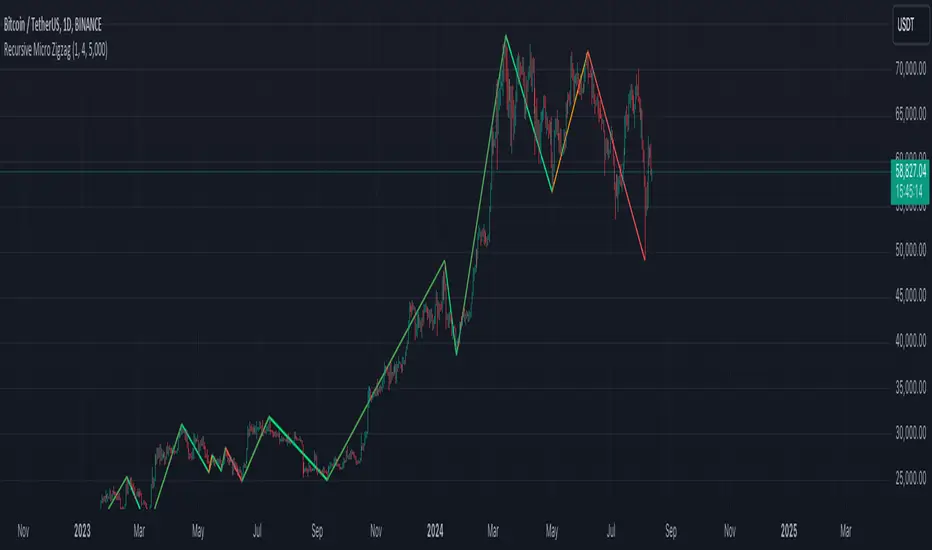
Recursive Micro Zigzag🎲 Overview
Zigzag is basic building block for any pattern recognition algorithm. This indicator is a research-oriented tool that combines the concepts of Micro Zigzag and Recursive Zigzag to facilitate a comprehensive analysis of price patterns. This indicator focuses on deriving zigzag on multiple levels in more efficient and enhanced manner in order to support enhanced pattern recognition.
The Recursive Micro Zigzag Indicator utilises the Micro Zigzag as the foundation and applies the Recursive Zigzag technique to derive higher-level zigzags. By integrating these techniques, this indicator enables researchers to analyse price patterns at multiple levels and gain a deeper understanding of market behaviour.
🎲 Concept:
Micro Zigzag Base : The indicator utilises the Micro Zigzag concept to capture detailed price movements within each candle. It allows for the visualisation of the sequential price action within the candle, aiding in pattern recognition at a micro level.
Basic implementation of micro zigzag can be found in this link - Micro-Zigzag
Recursive Zigzag Expansion : Building upon the Micro Zigzag base, the indicator applies the Recursive Zigzag concept to derive higher-level zigzags. Through recursive analysis of the Micro Zigzag's pivots, the indicator uncovers intricate patterns and trends that may not be evident in single-level zigzags.
Earlier implementations of recursive zigzag can be found here:
Recursive Zigzag
Recursive Zigzag - Trendoscope
And the libraries
rZigzag
ZigzagMethods
The major differences in this implementation are
Micro Zigzag Base - Earlier implementation made use of standard zigzag as base whereas this implementation uses Micro Zigzag as base
Not cap on Pivot depth - Earlier implementation was limited by the depth of level 0 zigzag. In this implementation, we are trying to build the recursive algorithm progressively so that there is no cap on the depth of level 0 zigzag. But, if we go for higher levels, there is chance of program timing out due to pine limitations.
These algorithms are useful in automatically spotting patterns on the chart including Harmonic Patterns, Chart Patterns, Elliot Waves and many more.
Smart Money Concepts Probability (Expo)█ Overview
The Smart Money Concept Probability (Expo) is an indicator developed to track the actions of institutional investors, commonly known as "smart money." This tool calculates the likelihood of smart money being actively engaged in buying or selling within the market, referred to as the "smart money order flow."
The indicator measures the probability of three key events: Change of Character ( CHoCH ), Shift in Market Structure ( SMS ), and Break of Structure ( BMS ). These probabilities are displayed as percentages alongside their respective levels, providing a straightforward and immediate understanding of the likelihood of smart money order flow.
Finally, the backtested results are shown in a table, which gives traders an understanding of the historical performance of the current order flow direction.
█ Calculations
The algorithm individually computes the likelihood of the events ( CHoCH , SMS , and BMS ). A positive score is assigned for events where the price successfully breaks through the level with the highest probability, and a negative score when the price fails to do so. By doing so, the algorithm determines the probability of each event occurring and calculates the total profitability derived from all the events.
█ Example
In this case, we have an 85% probability that the price will break above the upper range and make a new Break Of Structure and only a 16.36% probability that the price will break below the lower range and make a Change Of Character.
█ Settings
The Structure Period sets the pivot period to use when calculating the market structure.
The Structure Response sets how responsive the market structure should be. A low value returns a more responsive structure. A high value returns a less responsive structure.
█ How to use
This indicator is a perfect tool for anyone that wants to understand the probability of a Change of Character ( CHoCH ), Shift in Market Structure ( SMS ), and Break of Structure ( BMS )
The insights provided by this tool help traders gain an understanding of the smart money order flow direction, which can be used to determine the market trend.
█ Any Alert function call
An alert is sent when the price breaks the upper or lower range, and you can select what should be included in the alert. You can enable the following options:
Ticker ID
Timeframe
Probability percentage
-----------------
Disclaimer
The information contained in my Scripts/Indicators/Ideas/Algos/Systems does not constitute financial advice or a solicitation to buy or sell any securities of any type. I will not accept liability for any loss or damage, including without limitation any loss of profit, which may arise directly or indirectly from the use of or reliance on such information.
All investments involve risk, and the past performance of a security, industry, sector, market, financial product, trading strategy, backtest, or individual's trading does not guarantee future results or returns. Investors are fully responsible for any investment decisions they make. Such decisions should be based solely on an evaluation of their financial circumstances, investment objectives, risk tolerance, and liquidity needs.
My Scripts/Indicators/Ideas/Algos/Systems are only for educational purposes!

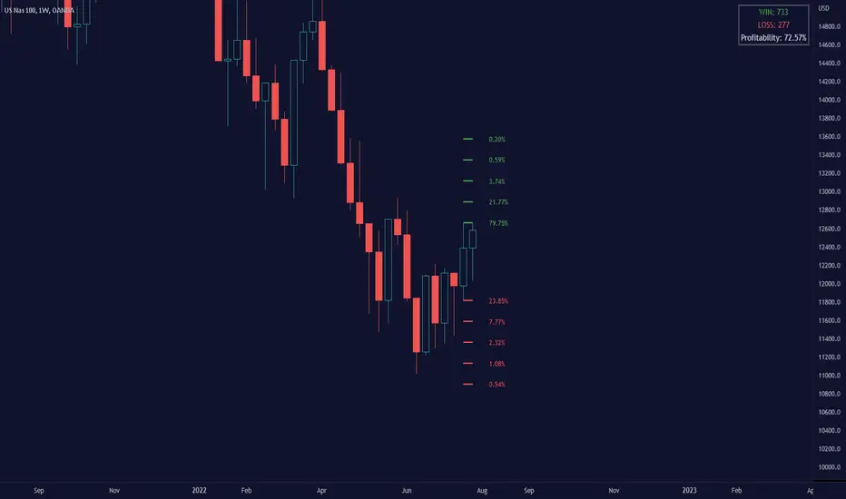
Breakout Probability (Expo)█ Overview
Breakout Probability is a valuable indicator that calculates the probability of a new high or low and displays it as a level with its percentage. The probability of a new high and low is backtested, and the results are shown in a table— a simple way to understand the next candle's likelihood of a new high or low. In addition, the indicator displays an additional four levels above and under the candle with the probability of hitting these levels.
The indicator helps traders to understand the likelihood of the next candle's direction, which can be used to set your trading bias.
█ Calculations
The algorithm calculates all the green and red candles separately depending on whether the previous candle was red or green and assigns scores if one or more lines were reached. The algorithm then calculates how many candles reached those levels in history and displays it as a percentage value on each line.
█ Example
In this example, the previous candlestick was green; we can see that a new high has been hit 72.82% of the time and the low only 28.29%. In this case, a new high was made.
█ Settings
Percentage Step
The space between the levels can be adjusted with a percentage step. 1% means that each level is located 1% above/under the previous one.
Disable 0.00% values
If a level got a 0% likelihood of being hit, the level is not displayed as default. Enable the option if you want to see all levels regardless of their values.
Number of Lines
Set the number of levels you want to display.
Show Statistic Panel
Enable this option if you want to display the backtest statistics for that a new high or low is made. (Only if the first levels have been reached or not)
█ Any Alert function call
An alert is sent on candle open, and you can select what should be included in the alert. You can enable the following options:
Ticker ID
Bias
Probability percentage
The first level high and low price
█ How to use
This indicator is a perfect tool for anyone that wants to understand the probability of a breakout and the likelihood that set levels are hit.
The indicator can be used for setting a stop loss based on where the price is most likely not to reach.
The indicator can help traders to set their bias based on probability. For example, look at the daily or a higher timeframe to get your trading bias, then go to a lower timeframe and look for setups in that direction.
-----------------
Disclaimer
The information contained in my Scripts/Indicators/Ideas/Algos/Systems does not constitute financial advice or a solicitation to buy or sell any securities of any type. I will not accept liability for any loss or damage, including without limitation any loss of profit, which may arise directly or indirectly from the use of or reliance on such information.
All investments involve risk, and the past performance of a security, industry, sector, market, financial product, trading strategy, backtest, or individual's trading does not guarantee future results or returns. Investors are fully responsible for any investment decisions they make. Such decisions should be based solely on an evaluation of their financial circumstances, investment objectives, risk tolerance, and liquidity needs.
My Scripts/Indicators/Ideas/Algos/Systems are only for educational purposes!
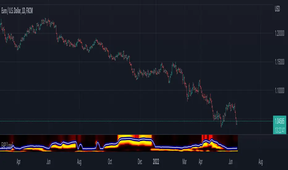
FATL, SATL, RFTL, & RSTL Digital Signal Filter Smoother [Loxx]FATL, SATL, RFTL, & RSTL Digital Signal Filter (DSP) Smoother is is a baseline indicator with DSP processed source inputs
What are digital indicators: distinctions from standard tools, types of filters.
To date, dozens of technical analysis indicators have been developed: trend instruments, oscillators, etc. Most of them use the method of averaging historical data, which is considered crude. But there is another group of tools - digital indicators developed on the basis of mathematical methods of spectral analysis. Their formula allows the trader to filter price noise accurately and exclude occasional surges, making the forecast more effective in comparison with conventional indicators. In this review, you will learn about their distinctions, advantages, types of digital indicators and examples of strategies based on them.
Two non-standard strategies based on digital indicators
Basic technical analysis indicators built into most platforms are based on mathematical formulas. These formulas are a reflection of market behavior in past periods. In other words, these indicators are built based on patterns that were discovered as a result of statistical analysis, which allows one to predict further trend movement to some extent. But there is also a group of indicators called digital indicators. They are developed using mathematical analysis and are an algorithmic spectral system called ATCF (Adaptive Trend & Cycles Following). In this article, I will tell you more about the components of this system, describe the differences between digital and regular indicators, and give examples of 2 strategies with indicator templates.
ATCF - Market Spectrum Analysis Method
There is a theory according to which the market is chaotic and unpredictable, i.e. it cannot be accurately analyzed. After all, no one can tell how traders will react to certain news, or whether some large investor will want to play against the market like George Soros did with the Bank of England. But there is another theory: many general market trends are logical, and have a rationale, causes and effects. The economy is undulating, which means it can be described by mathematical methods.
Digital indicators are defined as a group of algorithms for assessing the market situation, which are based exclusively on mathematical methods. They differ from standard indicators by the form of analysis display. They display certain values: price, smoothed price, volumes. Many standard indicators are built on the basis of filtering the minute significant price fluctuations with the help of moving averages and their variations. But we can hardly call the MA a good filter, because digital indicators that use spectral filters make it possible to do a more accurate calculation.
Simply put, digital indicators are technical analysis tools in which spectral filters are used to filter out price noise instead of moving averages.
The display of traditional indicators is lines, areas, and channels. Digital indicators can be displayed both in the form of lines and in digital form (a set of numbers in columns, any data in a text field, etc.). The digital display of the data is more like an additional source of statistics; for trading, a standard visual linear chart view is used.
All digital models belong to the category of spectral analysis of the market situation. In conventional technical indicators, price indications are averaged over a fixed period of time, which gives a rather rough result. The use of spectral analysis allows us to increase trading efficiency due to the fact that digital indicators use a statistical data set of past periods, which is converted into a “frequency” of the market (period of fluctuations).
Fourier theory provides the following spectral ranging of the trend duration:
low frequency range (0-4) - a reflection of a long trend of 2 months or more
medium frequency range (5-40) - the trend lasts 10-60 days, thus it is referred to as a correction
high frequency range (41-130) - price noise that lasts for several days
The ATCF algorithm is built on the basis of spectral analysis and includes a set of indicators created using digital filters. Its consists of indicators and filters:
FATL: Built on the basis of a low-frequency digital trend filter
SATL: Built on the basis of a low-frequency digital trend filter of a different order
RFTL: High frequency trend line
RSTL: Low frequency trend line
Inclucded:
4 DSP filters
Bar coloring
Keltner channels with variety ranges and smoothing functions
Bollinger bands
40 Smoothing filters
33 souce types
Variable channels

Ehlers Autocorrelation Periodogram [Loxx]Ehlers Autocorrelation Periodogram contains two versions of Ehlers Autocorrelation Periodogram Algorithm. This indicator is meant to supplement adaptive cycle indicators that myself and others have published on Trading View, will continue to publish on Trading View. These are fast-loading, low-overhead, streamlined, exact replicas of Ehlers' work without any other adjustments or inputs.
Versions:
- 2013, Cycle Analytics for Traders Advanced Technical Trading Concepts by John F. Ehlers
- 2016, TASC September, "Measuring Market Cycles"
Description
The Ehlers Autocorrelation study is a technical indicator used in the calculation of John F. Ehlers’s Autocorrelation Periodogram. Its main purpose is to eliminate noise from the price data, reduce effects of the “spectral dilation” phenomenon, and reveal dominant cycle periods. The spectral dilation has been discussed in several studies by John F. Ehlers; for more information on this, refer to sources in the "Further Reading" section.
As the first step, Autocorrelation uses Mr. Ehlers’s previous installment, Ehlers Roofing Filter, in order to enhance the signal-to-noise ratio and neutralize the spectral dilation. This filter is based on aerospace analog filters and when applied to market data, it attempts to only pass spectral components whose periods are between 10 and 48 bars.
Autocorrelation is then applied to the filtered data: as its name implies, this function correlates the data with itself a certain period back. As with other correlation techniques, the value of +1 would signify the perfect correlation and -1, the perfect anti-correlation.
Using values of Autocorrelation in Thermo Mode may help you reveal the cycle periods within which the data is best correlated (or anti-correlated) with itself. Those periods are displayed in the extreme colors (orange) while areas of intermediate colors mark periods of less useful cycles.
What is an adaptive cycle, and what is the Autocorrelation Periodogram Algorithm?
From his Ehlers' book mentioned above, page 135:
"Adaptive filters can have several different meanings. For example, Perry Kaufman’s adaptive moving average ( KAMA ) and Tushar Chande’s variable index dynamic average ( VIDYA ) adapt to changes in volatility . By definition, these filters are reactive to price changes, and therefore they close the barn door after the horse is gone.The adaptive filters discussed in this chapter are the familiar Stochastic , relative strength index ( RSI ), commodity channel index ( CCI ), and band-pass filter.The key parameter in each case is the look-back period used to calculate the indicator.This look-back period is commonly a fixed value. However, since the measured cycle period is changing, as we have seen in previous chapters, it makes sense to adapt these indicators to the measured cycle period. When tradable market cycles are observed, they tend to persist for a short while.Therefore, by tuning the indicators to the measure cycle period they are optimized for current conditions and can even have predictive characteristics.
The dominant cycle period is measured using the Autocorrelation Periodogram Algorithm. That dominant cycle dynamically sets the look-back period for the indicators. I employ my own streamlined computation for the indicators that provide smoother and easier to interpret outputs than traditional methods. Further, the indicator codes have been modified to remove the effects of spectral dilation.This basically creates a whole new set of indicators for your trading arsenal."
How to use this indicator
The point of the Ehlers Autocorrelation Periodogram Algorithm is to dynamically set a period between a minimum and a maximum period length. While I leave the exact explanation of the mechanic to Dr. Ehlers’s book, for all practical intents and purposes, in my opinion, the punchline of this method is to attempt to remove a massive source of overfitting from trading system creation–namely specifying a look-back period. SMA of 50 days? 100 days? 200 days? Well, theoretically, this algorithm takes that possibility of overfitting out of your hands. Simply, specify an upper and lower bound for your look-back, and it does the rest. In addition, this indicator tells you when its best to use adaptive cycle inputs for your other indicators.
Usage Example 1
Let's say you're using "Adaptive Qualitative Quantitative Estimation (QQE) ". This indicator has the option of adaptive cycle inputs. When the "Ehlers Autocorrelation Periodogram " shows a period of high correlation that adaptive cycle inputs work best during that period.
Usage Example 2
Check where the dominant cycle line lines, grab that output number and inject it into your other standard indicators for the length input.
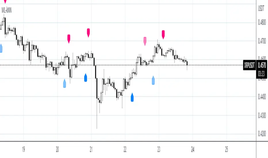
Machine Learning: kNN-based StrategykNN-based Strategy (FX and Crypto)
Description:
This strategy uses a classic machine learning algorithm - k Nearest Neighbours (kNN) - to let you find a prediction for the next (tomorrow's, next month's, etc.) market move. Being an unsupervised machine learning algorithm, kNN is one of the most simple learning algorithms.
To do a prediction of the next market move, the kNN algorithm uses the historic data, collected in 3 arrays - feature1, feature2 and directions, - and finds the k-nearest
neighbours of the current indicator(s) values.
The two dimensional kNN algorithm just has a look on what has happened in the past when the two indicators had a similar level. It then looks at the k nearest neighbours,
sees their state and thus classifies the current point.
The kNN algorithm offers a framework to test all kinds of indicators easily to see if they have got any *predictive value*. One can easily add cog, wpr and others.
Note: TradingViews's playback feature helps to see this strategy in action.
Warning: Signals ARE repainting.
Style tags: Trend Following, Trend Analysis
Asset class: Equities, Futures, ETFs, Currencies and Commodities
Dataset: FX Minutes/Hours+++/Days
Relative Strength(RSMK) + Perks - Markos KatsanosIf you are desperately looking for a novel RSI, this isn't that. This is another lesser known novel species of indicator. Hot off the press, in multiple stunning color schemes, I present my version of "Relative Strength (RSMK)" employing PSv4.0, originally formulated by Markos Katsanos for TASC - March 2020 Traders Tips. This indicator is used to compare performance of an asset to a market index of your choosing. I included the S&P 500 index along side the Dow Jones and the NASDAQ indices selectively by an input() in "Settings". You may comparatively analyze other global market indices by adapting the code, if you are skilled enough in Pine to do so.
With this contribution to the Tradingview community, also included is MY twin algorithmic formulation of "Comparative Relative Strength" as a supplementary companion indicator. They are eerily similar, so I decided to include it. You may easily disable my algorithm within the indicator "Settings". I do hope you may find both of them useful. Configurations are displayed above in multiple scenarios that should be suitable for most traders.
As always, I have included advanced Pine programming techniques that conform to proper "Pine Etiquette". For those of you who are newcomers to Pine Script, this script may also help you understand advanced programming techniques in Pine and how they may be utilized in a most effective manner. Utilizing the "Power of Pine", I included the maximum amount of features I could surmise in an ultra small yet powerful package, being less than a 60 line implementation at initial release.
Unfortunately, there are so many Pine mastery techniques included, I don't have time to write about all of them. I will have to let you discover them for yourself, excluding the following Pine "Tricks and Tips" described next. Of notable mention with this release, I have "overwritten" the Pine built-in function ema(). You may overwrite other built-in functions too. If you weren't aware of this Pine capability, you now know! Just heed caution when doing so to ensure your replacement algorithms are 100% sound. My ema() will also accept a floating point number for the period having ultimate adjustability. Yep, you heard all of that properly. Pine is becoming more impressive than `impressive` was originally thought of...
Features List Includes:
Dark Background - Easily disabled in indicator Settings->Style for "Light" charts or with Pine commenting
AND much, much more... You have the source!
The comments section below is solely just for commenting and other remarks, ideas, compliments, etc... regarding only this indicator, not others. When available time provides itself, I will consider your inquiries, thoughts, and concepts presented below in the comments section, should you have any questions or comments regarding this indicator. When my indicators achieve more prevalent use by TV members, I may implement more ideas when they present themselves as worthy additions. As always, "Like" it if you simply just like it with a proper thumbs up, and also return to my scripts list occasionally for additional postings. Have a profitable future everyone!
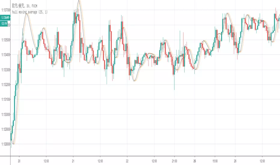
the "fasle" hull moving averageThere is a little different between my "fasle hull moving average" the "correct one".
the correct algorithm:
hma = wma((2*wma(close,n/2) - wma(close,n),sqrt(n))
the "fasle" algorithm:
=wma((2*wma(close,n/4) - wma(close,n),sqrt(n))
Amazing! Why the "fasle" describe the trend so accurate!?
MACD, backtest 2015+ only, cut in half and doubledThis is only a slight modification to the existing "MACD Strategy" strategy plugin!
found the default MACD strategy to be lacking, although impressive for its simplicity. I added "year>2014" to the IF buy/sell conditions so it will only backtest from 2015 and beyond ** .
I also had a problem with the standard MACD trading late, per se. To that end I modified the inputs for fast/slow/signal to double. Example: my defaults are 10, 21, 10 so I put 20, 42, 20 in. This has the effect of making a 30min interval the same as 1 hour at 10,21,10. So if you want to backtest at 4hr, you would set your time interval to 2hr on the main chart. This is a handy way to make shorter time periods more useful even regardless of strategy/testing, since you can view 15min with alot less noise but a better response.
Used on BTCCNY OKcoin, with the chart set at 45 min (so really 90min in the strategy) this gave me a percent profitable of 42% and a profit factor of 1.998 on 189 trades.
Personally, I like to set the length/signals to 30,63,30. Meaning you need to triple the time, it allows for much better use of shorter time periods and the backtests are remarkably profitable. (i.e. 15min chart view = 45min on script, 30min= 1.5hr on script)
** If you want more specific time periods you need to try plugging in different bar values: replace "year" with "n" and "2014" with "5500". The bars are based on unix time I believe so you will need to play around with the number for n, with n being the numbers of bars.

Timeframe-Independent Anchored VWAPAn anchored VWAP (Volume Weighted Average Price) that produces identical values (down to the tick!) across different timeframes (unlike, for example, TradingView's built-in Anchored VWAP).
Advantages
This indicator calculates identical values whether you view it on 1m, 5m, 15m, or any other timeframe within reasonable ranges. Even challenging non-integer timeframe ratios like calculating on 2m while viewing on 3m are handled perfectly. In High or Low mode, VWAP will anchor precisely at the selected candle's high/low. As usual for AVWAP, up to 3 standard deviation bands are supported.
How to Use
Setting the Anchor: When the indicator is added, select your anchor time. This is typically placed at a significant swing high/low or session open.
Source Selection: Choose whether to anchor from High, Low, or Close price.
Calculation Timeframe: Select the timeframe used for VWAP calculation.
For intraday trading (1m-1H charts): Just keep the default setting (1m)
For swing trading (4H-D charts): Use 5m or 15m calculation timeframe
For position trading (D-W charts): Use 1H calculation timeframe
Important: Lower calculation timeframes provide more precise data but may hit Pine Script's bar limit on very long timeframes
Standard Deviation Bands: Enable additional band sets as needed for your trading style.
Technical Implementation
The indicator achieves timeframe independence through the following algorithm:
Lower Timeframe Sampling: Uses Pine Script's request.security_lower_tf() to retrieve bar data at the specified calculation timeframe, regardless of the viewing timeframe. This provides consistent data resolution across all chart timeframes.
Anchor Detection: Scans the lower timeframe data to identify the exact bar containing the selected anchor price. The algorithm handles both simple cases (where anchor falls on a complete bar) and complex cases (where anchor falls within a split bar in non-integer timeframe ratios like calculating on 2m while viewing on 3m).
FIFO Buffer Management: Maintains a First-In-First-Out buffer of lower timeframe bars. On each chart bar:
Adds new lower timeframe bars to the buffer
Processes exactly one period worth of bars (matching the viewing timeframe)
Removes processed bars from the buffer
This approach ensures consistent calculation regardless of viewing timeframe.
First Bar Initialization: On the anchor bar, processes only the single anchor bar to ensure the VWAP starts exactly at the anchor price. Subsequent bars process the full period, maintaining mathematical accuracy.
VWAP Calculation: Applies the standard volume-weighted average price formula:
VWAP = Σ(Price × Volume) / Σ(Volume)
StdDev = √(Σ(Price² × Volume) / Σ(Volume) - VWAP²)
All calculations accumulate from the anchor point forward.
Visual Continuity: For edge cases where the anchor falls in an incomplete bar (e.g., calculating on 2m while viewing on 3m), displays the anchor price as a visual placeholder until the actual calculation begins on the next bar. This ensures the line always starts visually at the anchor point.

RSI Fibonacci Flow [JOAT]RSI Fibonacci Flow - Advanced Fibonacci Retracement with RSI Confluence
Introduction
RSI Fibonacci Flow is an open-source overlay indicator that combines automatic Fibonacci retracement levels with RSI momentum analysis to identify high-probability trading zones. The indicator automatically detects swing highs and lows, draws Fibonacci levels, and generates confluence signals when RSI conditions align with key Fibonacci zones.
This indicator is designed for traders who use Fibonacci retracements but want additional confirmation from momentum analysis before entering trades.
Originality and Purpose
This indicator is NOT a simple mashup of RSI and Fibonacci tools. It is an original implementation that creates a synergistic relationship between two complementary analysis methods:
Why Combine RSI with Fibonacci? Fibonacci retracements identify WHERE price might reverse, but they don't tell you WHEN. RSI provides the timing component by showing momentum exhaustion. When price reaches the Golden Zone (50%-61.8%) AND RSI shows oversold conditions, the probability of a successful bounce increases significantly.
Original Confluence Scoring System: The indicator calculates a 0-5 confluence score that weights multiple factors: Golden Zone presence (+2), entry zone presence (+1), RSI extreme alignment (+1), RSI divergence (+1), and strong RSI momentum (+1). This scoring system is original to this indicator.
Automatic Pivot Detection: Unlike manual Fibonacci tools, this indicator automatically detects swing highs and lows using a configurable pivot algorithm, then draws Fibonacci levels accordingly. The pivot detection uses a center-bar comparison method that checks if a bar's high/low is the highest/lowest within the specified depth on both sides.
Dynamic Trend Awareness: The indicator determines trend direction based on pivot sequence (last pivot was high or low) and adjusts Fibonacci orientation accordingly. In uptrends, 0% is at swing low; in downtrends, 0% is at swing high.
Each component serves a specific purpose:
Fibonacci levels identify potential reversal zones based on natural price ratios
RSI provides momentum context to filter out low-probability setups
Confluence scoring quantifies setup quality for position sizing decisions
Automatic pivot detection removes subjectivity from level placement
Core Concept: RSI-Fibonacci Confluence
The most powerful trading setups occur when multiple factors align. RSI Fibonacci Flow identifies these moments by:
Automatically detecting price pivots and drawing Fibonacci levels
Tracking which Fibonacci zone the current price occupies
Monitoring RSI for overbought/oversold conditions
Generating signals when RSI extremes coincide with key Fibonacci levels
Scoring confluence strength on a 0-5 scale
When price reaches the Golden Zone (50%-61.8%) while RSI shows oversold conditions in an uptrend, the probability of a bounce increases significantly.
Fibonacci Levels Explained
The indicator draws nine Fibonacci levels based on the most recent swing:
0% (Swing Low/High): The starting point of the move
23.6%: Shallow retracement - often seen in strong trends
38.2%: First significant support/resistance level
50%: Psychological midpoint of the move
61.8% (Golden Ratio): The most important Fibonacci level
78.6%: Deep retracement - last defense before trend failure
100% (Swing High/Low): The end point of the move
127.2% (TP1): First extension target for take profit
161.8% (TP2): Second extension target for take profit
The Golden Zone
The area between 50% and 61.8% is highlighted as the "Golden Zone" because:
It represents the optimal retracement depth for trend continuation
Institutional traders often place orders in this zone
It offers favorable risk-to-reward ratios
Price frequently bounces from this area in healthy trends
When price enters the Golden Zone, the indicator highlights it with a semi-transparent box and optional background coloring.
Pivot Detection System
The indicator uses a configurable pivot detection algorithm:
pivotDetect(float src, int len, bool isHigh) =>
int halfLen = len / 2
float centerVal = nz(src , src)
bool isPivot = true
for i = 0 to len - 1
if isHigh
if nz(src , src) > centerVal
isPivot := false
break
else
if nz(src , src) < centerVal
isPivot := false
break
isPivot ? centerVal : float(na)
This identifies swing highs and lows by checking if a bar's high/low is the highest/lowest within the specified depth on both sides.
Visual Components
1. Fibonacci Lines
Horizontal lines at each Fibonacci level:
Solid lines for major levels (0%, 50%, 61.8%, 100%)
Dashed lines for secondary levels (23.6%, 38.2%, 78.6%)
Dotted lines for extension levels (127.2%, 161.8%)
Color-coded for easy identification
Configurable line width
2. Fibonacci Labels
Price labels at each level showing:
Fibonacci percentage
Actual price at that level
Golden Zone label highlighted
TP1 and TP2 labels for targets
3. Golden Zone Box
A semi-transparent box highlighting the 50%-61.8% zone:
Gold colored border and fill
Extends from swing start to current bar (or beyond if extended)
Provides clear visual of the optimal entry zone
4. ZigZag Lines
Connecting lines between detected pivots:
Cyan for moves from low to high
Orange for moves from high to low
Helps visualize market structure
Configurable line width
5. Pivot Markers
Small labels at detected swing points:
"HH" (Higher High) at swing highs
"LL" (Lower Low) at swing lows
Helps track market structure
6. Entry Signals
BUY and SELL labels when confluence conditions are met:
BUY: RSI oversold + price in entry zone + uptrend + positive momentum
SELL: RSI overbought + price in entry zone + downtrend + negative momentum
Labels include "RSI+FIB" to indicate confluence
Confluence Scoring System
The indicator calculates a confluence score from 0 to 5:
+2 points: Price is in the Golden Zone (50%-61.8%)
+1 point: Price is in the entry zone (38.2%-61.8%)
+1 point: RSI is oversold in uptrend OR overbought in downtrend
+1 point: RSI divergence detected (bullish or bearish)
+1 point: Strong RSI momentum (change > 2 points)
Confluence ratings:
STRONG (4-5): Multiple factors align - high probability setup
MODERATE (2-3): Some factors align - proceed with caution
WEAK (0-1): Few factors align - wait for better setup
Dashboard Panel
The 10-row dashboard provides comprehensive analysis:
RSI Value: Current RSI reading (large text)
RSI State: OVERBOUGHT, OVERSOLD, BULLISH, BEARISH, or NEUTRAL
Fib Trend: UPTREND or DOWNTREND based on last pivot sequence
Price Zone: Current Fibonacci zone (e.g., "GOLDEN ZONE", "38.2% - 50%")
Price: Current close price (large text)
Confluence: Score rating with numeric value (e.g., "STRONG (4/5)")
Nearest Fib: Closest key Fibonacci level with price
TP1 (127.2%): First take profit target price
TP2 (161.8%): Second take profit target price
Input Parameters
Pivot Detection:
Pivot Depth: Bars to look back for swing detection (default: 10)
Min Deviation %: Minimum price move to confirm pivot (default: 1.0)
RSI Settings:
RSI Length: Period for RSI calculation (default: 14)
Source: Price source (default: close)
Overbought: Upper threshold (default: 70)
Oversold: Lower threshold (default: 30)
Fibonacci Display:
Show Fib Lines: Toggle Fibonacci lines (default: enabled)
Show Fib Labels: Toggle price labels (default: enabled)
Show Golden Zone Box: Toggle zone highlight (default: enabled)
Line Width: Thickness of Fibonacci lines (default: 2)
Extend Fib Lines: Extend lines into future (default: enabled)
ZigZag:
Show ZigZag: Toggle connecting lines (default: enabled)
ZigZag Width: Line thickness (default: 2)
Signals:
Show Entry Signals: Toggle BUY/SELL labels (default: enabled)
Show TP Levels: Toggle take profit in dashboard (default: enabled)
Show RSI-Fib Confluence: Toggle confluence analysis (default: enabled)
Dashboard:
Show Dashboard: Toggle information panel (default: enabled)
Position: Choose corner placement
Colors:
Bullish: Color for bullish elements (default: cyan)
Bearish: Color for bearish elements (default: orange)
Neutral: Color for neutral elements (default: gray)
Golden Zone: Color for Golden Zone highlight (default: gold)
How to Use RSI Fibonacci Flow
Identifying Entry Zones:
Wait for price to retrace to the 38.2%-61.8% zone
Check if RSI is approaching oversold (for longs) or overbought (for shorts)
Look for STRONG confluence rating in the dashboard
Enter when BUY or SELL signal appears
Setting Take Profit Targets:
TP1 at 127.2% extension for conservative target
TP2 at 161.8% extension for aggressive target
Consider scaling out at each level
Using the Price Zone:
"BELOW 23.6%" - Price hasn't retraced much; wait for deeper pullback
"23.6% - 38.2%" - Shallow retracement; strong trend continuation possible
"38.2% - 50%" - Good entry zone for trend trades
"GOLDEN ZONE" - Optimal entry zone; highest probability
"61.8% - 78.6%" - Deep retracement; trend may be weakening
"78.6% - 100%" - Very deep; trend reversal possible
"ABOVE/BELOW 100%" - Trend has likely reversed
Confluence Trading Strategy:
Only take trades with confluence score of 3 or higher
STRONG confluence (4-5) warrants larger position size
MODERATE confluence (2-3) warrants smaller position size
WEAK confluence (0-1) - wait for better setup
Alert Conditions
Ten alert conditions are available:
RSI-Fib BUY Signal: Strong bullish confluence detected
RSI-Fib SELL Signal: Strong bearish confluence detected
Price in Golden Zone: Price enters 50%-61.8% zone
New Pivot High: Swing high detected
New Pivot Low: Swing low detected
RSI Overbought: RSI crosses above overbought threshold
RSI Oversold: RSI crosses below oversold threshold
Bullish Divergence: Potential bullish RSI divergence
Bearish Divergence: Potential bearish RSI divergence
Strong Confluence: Confluence score reaches 4 or higher
Understanding Trend Direction
The indicator determines trend based on pivot sequence:
UPTREND: Last pivot was a low after a high (expecting move up)
DOWNTREND: Last pivot was a high after a low (expecting move down)
Fibonacci levels are drawn accordingly:
In uptrend: 0% at swing low, 100% at swing high
In downtrend: 0% at swing high, 100% at swing low
Bar Coloring
When confluence features are enabled:
Cyan bars on strong bullish signals
Orange bars on strong bearish signals
Gold-tinted bars when price is in Golden Zone
Best Practices
Use on 1H timeframe or higher for more reliable pivots
Adjust Pivot Depth based on timeframe (higher for longer timeframes)
Wait for price to enter Golden Zone before considering entries
Confirm RSI is in favorable territory before trading
Use extension levels (127.2%, 161.8%) for realistic profit targets
Combine with support/resistance and candlestick patterns
Higher confluence scores indicate higher probability setups
Limitations
Pivot detection has inherent lag (must wait for confirmation)
Fibonacci levels are subjective - different swings produce different levels
Works best in trending markets with clear swings
RSI can remain overbought/oversold in strong trends
Not all Golden Zone entries will be successful
The source code is open and available for review and modification.
Disclaimer
This indicator is provided for educational and informational purposes only. It is not financial advice. Trading involves substantial risk of loss. Past performance does not guarantee future results. Fibonacci levels are not guaranteed support/resistance - they are probability zones based on historical price behavior. Always conduct your own analysis and use proper risk management.
- Made with passion by officialjackofalltrades :D

Quarter Point Autopilot v2.0.0Hello traders,
I am pleased to release the Quarter Point Autopilot . This is a specialized structural framework designed to impose mathematical order on price action by synthesizing major market cycles with fractal geometric subdivisions.
Defining accurate Support and Resistance often presents a dilemma: rely on subjective, manually drawn lines that vary from trader to trader, or clutter charts with lagging moving averages. The Quarter Point Autopilot solves this by quantifying "Algorithmic Geometry." It eliminates subjectivity by projecting a universal grid based on the mathematical quarter-points that institutional algorithms utilize to execute orders.
📐 The Concept: Algorithmic Geometry
To the untrained eye, price movement can appear chaotic or random. However, professional analysis reveals that markets move in measured "Steps." Large institutions do not place orders at random numbers; they utilize specific mathematical fractions of a Major Cycle to manage liquidity.
This indicator is specifically engineered to visualize this hidden framework. By defining a "Major Cycle" (Point A and Point B), the script calculates the entire universe of the chart. It mathematically subdivides the range into Halves, Quarters, Eighths, and Sixteenths, highlighting the precise levels where price creates "Structure" and where algorithmic reactions are most likely to occur.
⚙️ The Autopilot Logic: Infinite Scroll
In previous iterations of quarter-theory tools, traders were forced to manually redraw grids as price expanded into new territories.
This version introduces the "Autopilot" engine ( current_base logic ). The script dynamically detects which "Block" price is currently trading within and automatically projects the grid forward and backward in real-time. Whether price rallies 1,000 points or drops 500, the mathematical subdivisions snap to the correct integer block immediately, ensuring you never trade without context.
📊 Fractal Hierarchy
Not all levels are created equal. The indicator uses a visual hierarchy to help you distinguish the strength of a level at a glance:
Major Cycle: The "Hard Deck" boundaries of the range (0% / 100%).
Half-Major: The Equilibrium of the cycle (50%).
Large Quarters: The standard deviation points (25% / 75%).
Mid & Small Quarters: The granular detail (Eighths and Sixteenths) for precision entries.
User Guide:
Simply input two "Major Cycle Points" (a significant High and Low) in the settings. The script calculates the "Step Size" and handles the rest, projecting the grid relative to current price action.
Settings Include:
Calculation Group: Set your Point A and Point B to define the grid size.
Visual Group: Toggle the upper/lower buffers and customize the lookback/lookforward lengths to keep your chart clean.
Label Group: Choose to see Level Names, Prices, or both.

Moon Phases & Declinations - Chronos Capital [BETA]High-Precision Lunar Cycles: Moon Phases & Declinations (Swiss Ephemeris)
Overview
This indicator provides institutional-grade astronomical data directly on your chart. Unlike standard scripts that use basic sine-wave approximations, this tool implements the **Swiss Ephemeris algorithm**, the gold standard for high-precision celestial calculations.
By tracking the Moon’s phases and its **Maximum/Minimum Declinations**, traders can identify potential "turning points" or "energy shifts" in market volatility often associated with lunar cycles.
---
Key Features
Ultra-High Precision: Calculations are accurate to within *seconds* of time, ensuring that the visual plot aligns perfectly with astronomical reality.
Moon Phase Tracking: Distinct markers for New Moon, Full Moon, and Quarters.
Lunar Declination Peaks: Automatically identifies when the moon reaches its *Maximum North* and *Maximum South* points (Lunar Extremes).
Customizable Visuals: Toggle between background highlights, vertical lines, or plot signals to suit your trading style.
---
Technical Accuracy
This script is built using a ported version of the Swiss Ephemeris
Positional Accuracy: Within 0.1 arcseconds.
Time Accuracy: Within **~1-2 seconds** of official JPL data.
Algorithm: Integration of the *ELP2000-85* lunar theory for maximum reliability over decades of historical data.
---
### **How to Use**
1. **Reversal Zones:** Watch for the Moon’s *Max/Min Declination* points, which often coincide with local tops or bottoms in trending markets.
2. **Volatility Shifts:** Use the *New Moon* and *Full Moon* markers to anticipate periods of increased or decreased market liquidity and volume.
3. **Confluence:** Best used in combination with your existing price action or momentum indicators to add a "time-based" filter to your entries.
*Disclaimer: This tool is for educational and analytical purposes only. Lunar cycles are a study of time-based correlation, not a guaranteed financial signal.*

Neosha Concept V4 (NY Time)
Imagine the financial market as a huge ocean. Millions of traders throw orders into it every second. But beneath all the noise, there is a powerful current that quietly controls where the waves move. That current is not a person, not a trader, and not random—it is an algorithm.
This algorithm is called the Interbank Price Delivery Algorithm (IPDA).
Think of it as the “navigation system” that guides price through the market.
IPDA has one job:
to move prices in a way that keeps the market efficient and liquid.
To do this, it constantly looks for two things:
1. Where liquidity is hiding
Liquidity is usually found above highs and below lows—where traders place stop losses. The algorithm moves price there first to collect that liquidity.
2. Where price became unbalanced
Sometimes price moves too fast and creates gaps or imbalances. IPDA returns to those areas later to “fix” the missing orders.
Once you start looking at the charts with this idea in mind, everything makes more sense:
Why price suddenly spikes above a high and crashes down
Why big moves leave gaps that price later fills
Why the market reverses right after taking stops
Why trends begin only after certain levels are hit
These are not accidents.
They are the algorithm doing its job.
Price moves in a repeating cycle:
Gather liquidity
Make a strong move (displacement)
Return to fix inefficiency
Deliver to the next target
Most beginners only see the candles.
But once you understand IPDA, you see the intention behind the candles.
Instead of guessing where price might go, you begin to understand why it moves there.
And once you understand the “why,” your trading becomes clearer, calmer, and far more accurate.

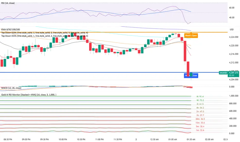
Gold AI RSI Monitor [Stacked + KNN]Here is a comprehensive description and user guide for the Gold AI RSI Monitor. You can copy and paste this into the "Description" field if you publish the script on TradingView, or save it for your own reference.
Gold AI RSI Monitor
🚀 Overview
The Gold AI RSI Monitor is a next-generation dashboard designed specifically for trading volatile assets like Gold (XAUUSD). It completely reimagines the traditional RSI by "stacking" 10 different timeframes (from 1-minute to Monthly) into a single, vertical view.
Integrated into this dashboard is a K-Nearest Neighbors (KNN) Machine Learning algorithm. This AI analyzes historical price action to find patterns similar to the current market and predicts the next likely move with a confidence score.
📊 Visual Guide: How to Read the Chart
1. The "Stacked" Lanes Instead of switching timeframes constantly, this indicator displays them all at once using vertical offsets.
Bottom Lane (0-100): 1-Minute RSI
Middle Lanes: 5m, 15m, 30m, 1H, 2H, 4H, Daily
Top Lane (900-1000): Monthly RSI
2. Gradient Color System The RSI lines change color based on momentum strength:
🔴 Red: Oversold / Bearish (Approaching 30 or lower)
🟡 Yellow: Neutral (Around 50)
🟢 Green: Overbought / Bullish (Approaching 70 or higher)
3. Tracker Lines Each timeframe has a dotted horizontal line extending to the right. This allows you to instantly see the exact RSI value for every timeframe without squinting.
🤖 The AI Engine (KNN)
The "AI" component uses a K-Nearest Neighbors algorithm.
Learning: It scans the last 1,000 bars of history.
Matching: It finds the 5 historical moments that look mathematically identical to the current market conditions (based on RSI and Volatility).
Predicting: It checks if price went UP or DOWN after those historical matches.
The Signals:
Buying Signal: If the majority of historical matches resulted in a price increase, the AI triggers a BUY.
Selling Signal: If the majority resulted in a drop, the AI triggers a SELL.
🎯 How to Trade with This Indicator
1. The "Crosshair" Signal
When the AI detects a high-probability setup, a massive Crosshair appears on your chart:
Green Crosshair: Strong BUY signal.
Red Crosshair: Strong SELL signal.
Note: The crosshair consists of a thick vertical line and a dashed horizontal line intersecting at the signal candle.
2. Timeframe Alignment (Confluence)
Do not rely on the AI alone. Look at the stacked RSIs:
Strong Long: The AI shows a Green Crosshair AND the lower timeframes (1m, 5m, 15m) are all turning Green/upward.
Strong Short: The AI shows a Red Crosshair AND the lower timeframes are turning Red/downward.
3. Support & Resistance Zones
Bottom Dotted Line (30): Support. If RSI hits this and turns up, it's a buying opportunity.
Top Dotted Line (70): Resistance. If RSI hits this and turns down, it's a selling opportunity.
⚙️ Settings Guide
RSI Length: Default is 14. Lower (e.g., 7) makes it faster/choppier; higher (e.g., 21) makes it smoother.
Enable AI Signals: Toggles the KNN calculation on/off.
Neighbors (K): How many historical matches to check. Default is 5.
Increase to 9-10 for fewer, more conservative signals.
Decrease to 3 for faster, more aggressive signals.
AI Timeframe: CRITICAL SETTING.
If left empty, the AI calculates based on your current chart.
Recommendation: For Gold scalping, set this to 15m or 1h. This ensures the AI looks at the bigger trend even if you are zooming in on the 1-minute chart.
⚠️ Disclaimer
This tool is for educational and analytical purposes. The "AI" is a statistical probability algorithm based on past performance, which is not indicative of future results. Always manage your risk.
RCV Essentials════════════════════════════════════════════
RCV ESSENTIALS - MULTI-TIMEFRAME & SESSION ANALYSIS TOOL
════════════════════════════════════════════
📊 WHAT THIS INDICATOR DOES
This professional-grade indicator combines two powerful analysis modules:
1. TRADING SESSION TRACKER - Visualizes high/low ranges for major global market sessions (NY Open, London Open, Asian Session, etc.)
2. MULTI-TIMEFRAME CANDLE DISPLAY - Shows up to 8 higher timeframes simultaneously on your chart (15m, 30m, 1H, 4H, 1D, 1W, 1M, 3M)
════════════════════════════════════════════
🎯 KEY FEATURES
════════════════════════════════════════════
TRADING SESSIONS MODULE:
✓ Track up to 6 custom trading sessions simultaneously
✓ Real-time high/low range detection during active sessions
✓ Pre-configured for NYO (7-9am), LNO (2-3am), Asian Session (4:30pm-12am)
✓ 60+ global timezone options
✓ Customizable colors, labels, and transparency
✓ Daily divider lines (optional Sunday skip for traditional markets)
✓ Only displays on ≤30m timeframes for optimal clarity
MULTI-TIMEFRAME CANDLES MODULE:
✓ Display 1-8 higher timeframes with up to 10 candles each
✓ Real-time candle updates (non-repainting)
✓ Fully customizable colors (separate bullish/bearish for body/border/wick)
✓ Adjustable candle width, spacing, and positioning
✓ Smart label system (top/bottom/both, aligned or follow candles)
✓ Automatic timeframe validation (only shows TFs higher than chart)
✓ Memory-optimized with automatic cleanup
════════════════════════════════════════════
🔧 HOW IT WORKS
════════════════════════════════════════════
TECHNICAL IMPLEMENTATION:
Session Tracking Algorithm:
• Detects session start/end using time() function with timezone support
• Continuously monitors and updates high/low during active session
• Finalizes range when session ends using var persistence
• Draws boxes using real-time bar_index positioning
• Maintains session ranges across multiple days for reference
Multi-Timeframe System:
• Uses ta.change(time()) detection to identify new MTF candle formation
• Constructs candles using custom Type definitions (Candle, CandleSet, Config)
• Stores OHLC data in arrays with automatic size management
• Renders using box objects (bodies) and line objects (wicks)
• Updates current candle every tick; historical candles remain static
• Calculates dynamic positioning based on user settings (offset, spacing, width)
Object-Oriented Architecture:
• Custom Type "Candle" - Stores OHLC values, timestamps, visual elements
• Custom Type "CandleSet" - Manages arrays of candles + settings per timeframe
• Custom Type "Config" - Centralizes all display configuration
• Efficient memory management via unshift() for new candles, pop() for old
Performance Optimizations:
• var declarations minimize recalculation overhead
• Conditional execution (sessions only on short timeframes)
• Maximum display limits prevent excessive object creation
• Timeframe validation at barstate.isfirst reduces redundant checks
════════════════════════════════════════════
📈 HOW TO USE
════════════════════════════════════════════
SETUP:
1. Add indicator to chart (works best on 1m-30m timeframes)
2. Open Settings → "Trading Sessions" group
- Enable desired sessions (NYO, LNO, AS, or custom)
- Select your timezone from 60+ options
- Adjust colors and transparency
3. Open Settings → "Multi-TF Candles" group
- Enable timeframes (TF1-TF8)
- Configure each timeframe and display count
- Customize colors and layout
READING THE CHART:
• Session boxes show high/low ranges during active sessions
• MTF candles display to the right of current price
• Labels identify each timeframe (15m, 1H, 4H, etc.)
• Real-time updates on the most recent MTF candle
TRADING APPLICATIONS:
Session Breakout Strategy:
→ Identify session high/low (e.g., Asian session 16:30-00:00)
→ Wait for break above/below range
→ Confirm with higher timeframe candle close
→ Enter in breakout direction, stop at opposite side of range
Multi-Timeframe Confirmation:
→ Spot setup on primary chart (e.g., 5m)
→ Verify 15m, 1H, 4H candles align with trade direction
→ Only take trades where higher TFs confirm
→ Exit when higher TF candles show reversal
Combined Session + MTF:
→ Asian session establishes range overnight
→ London Open breaks Asian high
→ Confirm with bullish 15m + 1H candles
→ Enter long with stop below Asian high
════════════════════════════════════════════
🎨 ORIGINALITY & INNOVATION
════════════════════════════════════════════
What makes this indicator original:
1. INTEGRATED DUAL-MODULE DESIGN
Unlike separate session or MTF indicators, this combines both in a single performance-optimized script, enabling powerful correlation analysis between session behavior and timeframe structure.
2. ADVANCED RENDERING SYSTEM
Uses custom Pine Script v5 Types with dynamic box/line object management instead of basic plot functions. This enables:
• Precise visual control over positioning and spacing
• Real-time updates without repainting
• Efficient memory handling via automatic cleanup
• Support for 8 simultaneous timeframes with independent settings
3. INTELLIGENT SESSION TRACKING
The algorithm continuously recalculates ranges bar-by-bar during active sessions, then preserves the final range. This differs from static zone indicators that simply draw fixed boxes at predefined levels.
4. MODULAR ARCHITECTURE
Custom Type definitions (Candle, CandleSet, Config) create extensible, maintainable code structure while supporting complex multi-timeframe operations with minimal performance impact.
5. PROFESSIONAL FLEXIBILITY
Extensive customization: 6 configurable sessions, 8 timeframe slots, 60+ timezones, granular color/sizing/spacing controls, multiple label positioning modes—adaptable to any market or trading style.
6. SMART VISUAL DESIGN
Automatic timeframe validation, dynamic label alignment options, and intelligent spacing calculations ensure clarity even with multiple timeframes displayed simultaneously.
════════════════════════════════════════════
⚙️ CONFIGURATION OPTIONS
════════════════════════════════════════════
TRADING SESSIONS:
• Session 1-6: On/Off toggles
• Time Ranges: Custom start-end times
• Labels: Custom text for each session
• Colors: Individual color per session
• Timezone: 60+ options (Americas, Europe, Asia, Pacific, Africa)
• Range Transparency: 0-100%
• Outline: Optional border
• Label Display: Show/hide session names
• Daily Divider: Dotted lines at day changes
• Skip Sunday: For traditional markets vs 24/7 crypto
MULTI-TF CANDLES:
• Timeframes 1-8: Enable/disable individually
• Timeframe Selection: Any TF (seconds to months)
• Display Count: 1-10 candles per timeframe
• Bullish Colors: Body/Border/Wick (independent)
• Bearish Colors: Body/Border/Wick (independent)
• Candle Width: 1-10+ bars
• Right Margin: 0-200+ bars from edge
• TF Spacing: Gap between timeframe groups
• Label Color: Any color
• Label Size: Tiny/Small/Normal/Large/Huge
• Label Position: Top/Bottom/Both
• Label Alignment: Follow Candles or Align
════════════════════════════════════════════
📋 TECHNICAL SPECIFICATIONS
════════════════════════════════════════════
• Pine Script Version: v5
• Chart Overlay: True
• Max Boxes: 500
• Max Lines: 500
• Max Labels: 500
• Max Bars Back: 5000
• Update Frequency: Real-time (every tick)
• Timeframe Compatibility: Chart TF must be lower than selected MTFs
• Session Display: Activates only on ≤30 minute timeframes
• Memory Management: Automatic cleanup via array operations

Pattern Match & Forward Projection – Weekly (EN)
Overview
This indicator searches for recurring price patterns in weekly data and projects their average forward performance.
The logic is based on historical pattern repetition: it scans past price sequences similar to the most recent one, then aggregates their forward returns to estimate potential outcomes.
⚠️ Important: The indicator is designed for weekly timeframe only. Using it on daily or intraday charts will trigger an error message.
Settings (Inputs)
Pattern Settings
Pattern length (weeks): Number of weeks used to define the reference pattern.
Forward length (weeks): Number of weeks into the future to evaluate after each pattern match.
Lookback (weeks): Historical window to scan for past pattern matches.
Normalize by shape (z-score): If enabled, patterns are normalized by z-score, focusing on shape similarity rather than absolute values.
Distance threshold (Euclidean): Maximum allowed Euclidean distance between the reference pattern and historical candidates. Smaller values = stricter matching.
Min. required matches: Minimum number of valid matches needed for analysis.
Quality Filters
Min required Hit%: Minimum percentage of positive outcomes (upside forward returns) required for the pattern to be considered valid.
Return filter mode:
Either: absolute average return ≥ threshold
Long only: average return ≥ threshold
Short only: average return ≤ -threshold
Min avg return (%): Minimum average forward return threshold for validation.
Visual Options
Highlight historical matches (labels): Marks where in history similar patterns occurred.
Max match labels to draw: Caps the number of match markers shown to avoid clutter.
Draw average projection: Displays the average projected forward curve if conditions are met.
Show summary panel: Enables/disables the information panel.
Show weekly avg curve in panel: Adds a breakdown of average returns week by week.
Projection color: Choose the color of the projected forward curve.
What the Screen Shows
Summary Panel (top-left by default)
Total matches found in history
Matches with valid forward data
Average, minimum, and maximum distance (similarity measure)
Average forward return and Hit%
Distance threshold and normalization setting
Weekly average forward curve (if enabled)
Quality filter results (pass/fail)
Projection Curve (dotted line on price chart)
Drawn only if enough valid matches are found and filters are satisfied
Represents the average forward performance of historical matches, anchored at the current bar
Historical Match Labels (▲ markers)
Small arrows below past bars where similar patterns occurred
Tooltip: “Historical match”
Forecast Logic
The indicator does not predict the future in a deterministic way.
Instead, it relies on a pattern-matching algorithm:
The most recent N weeks (defined by Pattern length) are taken as the reference.
The algorithm scans the last Lookback (weeks) for segments with similar shape and magnitude.
Similarity is measured using Euclidean distance (optionally z-score normalized).
For each valid match, the subsequent Forward length weeks are collected.
These forward paths are averaged to generate a composite forward projection.
The summary panel reports whether the current setup passes the quality filters (Hit% and minimum average return).
Usage Notes
Best used as a contextual tool, not a standalone trading system.
Works only on weekly timeframe.
Quality filters help distinguish between noisy and statistically meaningful patterns.
A higher number of matches usually improves reliability, but very strict thresholds may reduce sample size.
📊 This tool is useful for traders who want to evaluate how similar historical setups have behaved and to visualize potential forward paths in a statistically aggregated way.

主力资金进出监控器Main Capital Flow Monitor-MEWINSIGHTMain Capital Flow Monitor Indicator
Indicator Description
This indicator utilizes a multi-cycle composite weighting algorithm to accurately capture the movement of main capital in and out of key price zones. The core logic is built upon three dimensions:
Multi-Cycle Pressure/Support System
Using triple timeframes (500-day/250-day/90-day) to calculate:
Long-term resistance lines (VAR1-3): Monitoring historical high resistance zones
Long-term support lines (VAR4-6): Identifying historical low support zones
EMA21 smoothing is applied to eliminate short-term fluctuations
Dynamic Capital Activity Engine
Proprietary VARD volatility algorithm:
VARD = EMA
Automatically amplifies volatility sensitivity by 10x when price approaches the safety margin (VARA×1.35), precisely capturing abnormal main capital movements
Capital Inflow Trigger Mechanism
Capital entry signals require simultaneous fulfillment of:
Price touching 30-day low zone (VARE)
Capital activity breaking recent peaks (VARF)
Weighted capital flow verified through triple EMA:
Capital Entry = EMA / 618
Visualization:
Green histogram: Continuous main capital inflow
Red histogram: Abnormal daily capital movement intensity
Column height intuitively displays capital strength
Application Scenarios:
Consecutive green columns → Main capital accumulation at bottom
Sudden expansion of red columns → Abnormal main capital rush
Continuous fluctuations near zero axis → Main capital washing phase
Core Value:
Provides 1-3 trading days early warning of main capital movements, suitable for:
Medium/long-term investors identifying main capital accumulation zones
Short-term traders capturing abnormal main capital breakouts
Risk control avoiding main capital distribution phases
Parameter Notes: Default parameters are optimized through historical A-share market backtesting. Users can adjust cycle parameters according to different market characteristics (suggest extending cycles by 20% for European/American markets).
Formula Features:
Multi-timeframe weighted synthesis technology
Dynamic sensitivity adjustment mechanism
Main capital activity intensity quantification
Early warning function for capital movements
Suitable Markets:
Stocks, futures, cryptocurrencies and other financial markets with obvious main capital characteristics.
指标名称:主力资金进出监控器
指标描述:
本指标通过多周期复合加权算法,精准捕捉主力资金在关键价格区域的进出动向。核心逻辑基于三大维度构建:
多周期压力/支撑体系
通过500日/250日/90日三重时间框架,分别计算:
长期压力线(VAR1-3):监控历史高位阻力区
长期支撑线(VAR4-6):识别历史低位承接区
采用EMA21平滑处理,消除短期波动干扰
动态资金活跃度引擎
独创VARD波动率算法:
当价格接近安全边际(VARA×1.35)时自动放大波动敏感度10倍,精准捕捉主力异动
资金进场触发机制
资金入场信号需同时满足:
价格触及30日最低区域(VARE)
资金活跃度突破近期峰值(VARF)
通过三重EMA验证的加权资金流:
资金入场 = EMA / 618
可视化呈现:
绿色柱状图:主力资金持续流入
红色柱状图:当日资金异动量级
柱体高度直观显示资金强度
使用场景:
绿色柱体连续出现 → 主力底部吸筹
红色柱体突然放大 → 主力异动抢筹
零轴附近持续波动 → 主力洗盘阶段
核心价值:
提前1-3个交易日预警主力资金动向,适用于:
中长线投资者识别主力建仓区间
短线交易者捕捉主力异动突破
风险控制规避主力出货阶段
参数说明:默认参数经A股历史数据回测优化,用户可根据不同市场特性调整周期参数(建议欧美市场延长周期20%)
Composite Time ProfileComposite Time Profile Overlay (CTPO) - Market Profile Compositing Tool
Automatically composite multiple time periods to identify key areas of balance and market structure
What is the Composite Time Profile Overlay?
The Composite Time Profile Overlay (CTPO) is a Pine Script indicator that automatically composites multiple time periods to identify key areas of balance and market structure. It's designed for traders who use market profile concepts and need to quickly identify where price is likely to find support or resistance.
The indicator analyzes TPO (Time Price Opportunity) data across different timeframes and merges overlapping profiles to create composite levels that represent the most significant areas of balance. This helps you spot where institutional traders are likely to make decisions based on accumulated price action.
Why Use CTPO for Market Profile Trading?
Eliminate Manual Compositing Work
Instead of manually drawing and compositing profiles across different timeframes, CTPO does this automatically. You get instant access to composite levels without spending time analyzing each individual period.
Spot Areas of Balance Quickly
The indicator highlights the most significant areas of balance by compositing overlapping profiles. These areas often act as support and resistance levels because they represent where the most trading activity occurred across multiple time periods.
Focus on What Matters
Rather than getting lost in individual session profiles, CTPO shows you the composite levels that have been validated across multiple timeframes. This helps you focus on the levels that are most likely to hold.
How CTPO Works for Market Profile Traders
Automatic Profile Compositing
CTPO uses a proprietary algorithm that:
- Identifies period boundaries based on your selected timeframe (sessions, daily, weekly, monthly, or auto-detection)
- Calculates TPO profiles for each period using the C2M (Composite 2 Method) row sizing calculation
- Merges overlapping profiles using configurable overlap thresholds (default 50% overlap required)
- Updates composite levels as new price action develops in real-time
Key Levels for Market Profile Analysis
The indicator displays:
- Value Area High (VAH) and Value Area Low (VAL) levels calculated from composite TPO data
- Point of Control (POC) levels where most trading occurred across all composited periods
- Composite zones representing areas of balance with configurable transparency
- 1.618 Fibonacci extensions for breakout targets based on composite range
Multiple Timeframe Support
- Sessions: For intraday market profile analysis
- Daily: For swing trading with daily profiles
- Weekly: For position trading with weekly structure
- Monthly: For long-term market profile analysis
- Auto: Automatically selects timeframe based on your chart
Trading Applications for Market Profile Users
Support and Resistance Trading
Use composite levels as dynamic support and resistance zones. These levels often hold because they represent areas where significant trading decisions were made across multiple timeframes.
Breakout Trading
When composite levels break, they often lead to significant moves. The indicator calculates 1.618 Fibonacci extensions to give you clear targets for breakout trades.
Mean Reversion Strategies
Value Area levels represent the price range where most trading activity occurred. These levels often act as magnets, drawing price back when it moves too far from the mean.
Institutional Level Analysis
Composite levels represent areas where institutional traders have made significant decisions. These levels often hold more weight than traditional technical analysis levels because they're based on actual trading activity.
Key Features for Market Profile Traders
Smart Compositing Logic
- Automatic overlap detection using price range intersection algorithms
- Configurable overlap thresholds (minimum 50% overlap required for merging)
- Dead composite identification (profiles that become engulfed by newer composites)
- Real-time updates as new price action develops using barstate.islast optimization
Visual Customization
- Customizable colors for active, broken, and dead composites
- Adjustable transparency levels for each composite state
- Premium/Discount zone highlighting based on current price vs composite range
- TPO aggression coloring using TPO distribution analysis to identify buying/selling pressure
- Fibonacci level extensions with 1.618 target calculations based on composite range
Clean Chart Presentation
- Only shows the most relevant composite levels (maximum 10 active composites)
- Eliminates clutter from individual session profiles
- Focuses on areas of balance that matter most to current price action
Real-World Trading Examples
Day Trading with Session Composites
Use session-based composites to identify intraday areas of balance. The VAH and VAL levels often act as natural profit targets and stop-loss levels for scalping strategies.
Swing Trading with Daily Composites
Daily composites provide excellent swing trading levels. Look for price reactions at composite zones and use the 1.618 extensions for profit targets.
Position Trading with Weekly Composites
Weekly composites help identify major trend changes and long-term areas of balance. These levels often hold for months or even years.
Risk Management
Composite levels provide natural stop-loss levels. If a composite level breaks, it often signals a significant shift in market sentiment, making it an ideal place to exit losing positions.
Why Composite Levels Work
Composite levels work because they represent areas where significant trading decisions were made across multiple timeframes. When price returns to these levels, traders often remember the previous price action and make similar decisions, creating self-fulfilling prophecies.
The compositing process uses a proprietary algorithm that ensures only levels validated across multiple time periods are displayed. This means you're looking at levels that have proven their significance through actual market behavior, not just random technical levels.
Technical Foundation
The indicator uses TPO (Time Price Opportunity) data combined with price action analysis to identify areas of balance. The C2M row sizing method ensures accurate profile calculations, while the overlap detection algorithm (minimum 50% price range intersection) ensures only truly significant composites are displayed. The algorithm calculates row size based on ATR (Average True Range) divided by 10, then converts to tick size for precise level calculations.
How the Code Actually Works
1. Period Detection and ATR Calculation
The code first determines the appropriate timeframe based on your chart:
- 1m-5m charts: Session-based profiles
- 15m-2h charts: Daily profiles
- 4h charts: Weekly profiles
- 1D charts: Monthly profiles
For each period type, it calculates the number of bars needed for ATR calculation:
- Sessions: 540 minutes divided by chart timeframe
- Daily: 1440 minutes divided by chart timeframe
- Weekly: 7 days worth of minutes divided by chart timeframe
- Monthly: 30 days worth of minutes divided by chart timeframe
2. C2M Row Size Calculation
The code calculates True Range for each bar in the determined period:
- True Range = max(high-low, |high-prevClose|, |low-prevClose|)
- Averages all True Range values to get ATR
- Row Size = (ATR / 10) converted to tick size
- This ensures each TPO row represents a meaningful price movement
3. TPO Profile Generation
For each period, the code:
- Creates price levels from lowest to highest price in the range
- Each level is separated by the calculated row size
- Counts how many bars touch each price level (TPO count)
- Finds the level with highest count = Point of Control (POC)
- Calculates Value Area by expanding from POC until 68.27% of total TPO blocks are included
4. Overlap Detection Algorithm
When a new profile is created, the code checks if it overlaps with existing composites:
- Calculates overlap range = min(currentVAH, prevVAH) - max(currentVAL, prevVAL)
- Calculates current profile range = currentVAH - currentVAL
- Overlap percentage = (overlap range / current profile range) * 100
- If overlap >= 50%, profiles are merged into a composite
5. Composite Merging Logic
When profiles overlap, the code creates a new composite by:
- Taking the earliest start bar and latest end bar
- Using the wider VAH/VAL range (max of both profiles)
- Keeping the POC from the profile with more TPO blocks
- Marking the composite as "active" until price breaks through
6. Real-Time Updates
The code uses barstate.islast to optimize performance:
- Only recalculates on the last bar of each period
- Updates active composite with live price action if enabled
- Cleans up old composites to prevent memory issues
- Redraws all visual elements from scratch each bar
7. Visual Rendering System
The code uses arrays to manage drawing objects:
- Clears all lines/boxes arrays on every bar
- Iterates through composites array to redraw everything
- Uses different colors for active, broken, and dead composites
- Calculates 1.618 Fibonacci extensions for broken composites
Getting Started with CTPO
Step 1: Choose Your Timeframe
Select the period type that matches your trading style:
- Use "Sessions" for day trading
- Use "Daily" for swing trading
- Use "Weekly" for position trading
- Use "Auto" to let the indicator choose based on your chart timeframe
Step 2: Customize the Display
Adjust colors, transparency, and display options to match your charting preferences. The indicator offers extensive customization options to ensure it fits seamlessly into your existing analysis.
Step 3: Identify Key Levels
Look for:
- Composite zones (blue boxes) - major areas of balance
- VAH/VAL lines - value area boundaries
- POC lines - areas of highest trading activity
- 1.618 extension lines - breakout targets
Step 4: Develop Your Strategy
Use these levels to:
- Set entry points near composite zones
- Place stop losses beyond composite levels
- Take profits at 1.618 extension levels
- Identify trend changes when major composites break
Perfect for Market Profile Traders
If you're already using market profile concepts in your trading, CTPO eliminates the manual work of compositing profiles across different timeframes. Instead of spending time analyzing each individual period, you get instant access to the composite levels that matter most.
The indicator's automated compositing process ensures you're always looking at the most relevant areas of balance, while its real-time updates keep you informed of changes as they happen. Whether you're a day trader looking for intraday levels or a position trader analyzing long-term structure, CTPO provides the market profile intelligence you need to succeed.
Streamline Your Market Profile Analysis
Stop wasting time on manual compositing. Let CTPO do the heavy lifting while you focus on executing profitable trades based on areas of balance that actually matter.
Ready to Streamline Your Market Profile Trading?
Add the Composite Time Profile Overlay to your charts today and experience the difference that automated profile compositing can make in your trading performance.
Volume Profile Grid [Alpha Extract]A sophisticated volume distribution analysis system that transforms market activity into institutional-grade visual profiles, revealing hidden support/resistance zones and market participant behavior. Utilizing advanced price level segmentation, bullish/bearish volume separation, and dynamic range analysis, the Volume Profile Grid delivers comprehensive market structure insights with Point of Control (POC) identification, Value Area boundaries, and volume delta analysis. The system features intelligent visualization modes, real-time sentiment analysis, and flexible range selection to provide traders with clear, actionable volume-based market context.
🔶 Dynamic Range Analysis Engine
Implements dual-mode range selection with visible chart analysis and fixed period lookback, automatically adjusting to current market view or analyzing specified historical periods. The system intelligently calculates optimal bar counts while maintaining performance through configurable maximum limits, ensuring responsive profile generation across all timeframes with institutional-grade precision.
// Dynamic period calculation with intelligent caching
get_analysis_period() =>
if i_use_visible_range
chart_start_time = chart.left_visible_bar_time
current_time = last_bar_time
time_span = current_time - chart_start_time
tf_seconds = timeframe.in_seconds()
estimated_bars = time_span / (tf_seconds * 1000)
range_bars = math.floor(estimated_bars)
final_bars = math.min(range_bars, i_max_visible_bars)
math.max(final_bars, 50) // Minimum threshold
else
math.max(i_periods, 50)
🔶 Advanced Bull/Bear Volume Separation
Employs sophisticated candle classification algorithms to separate bullish and bearish volume at each price level, with weighted distribution based on bar intersection ratios. The system analyzes open/close relationships to determine volume direction, applying proportional allocation for doji patterns and ensuring accurate representation of buying versus selling pressure across the entire price spectrum.
🔶 Multi-Mode Volume Visualization
Features three distinct display modes for bull/bear volume representation: Split mode creates mirrored profiles from a central axis, Side by Side mode displays sequential bull/bear segments, and Stacked mode separates volumes vertically. Each mode offers unique insights into market participant behavior with customizable width, thickness, and color parameters for optimal visual clarity.
// Bull/Bear volume calculation with weighted distribution
for bar_offset = 0 to actual_periods - 1
bar_high = high
bar_low = low
bar_volume = volume
// Calculate intersection weight
weight = math.min(bar_high, next_level) - math.max(bar_low, current_level)
weight := weight / (bar_high - bar_low)
weighted_volume = bar_volume * weight
// Classify volume direction
if bar_close > bar_open
level_bull_volume += weighted_volume
else if bar_close < bar_open
level_bear_volume += weighted_volume
else // Doji handling
level_bull_volume += weighted_volume * 0.5
level_bear_volume += weighted_volume * 0.5
🔶 Point of Control & Value Area Detection
Implements institutional-standard POC identification by locating the price level with maximum volume accumulation, providing critical support/resistance zones. The Value Area calculation uses sophisticated sorting algorithms to identify the price range containing 70% of trading volume, revealing the market's accepted value zone where institutional participants concentrate their activity.
🔶 Volume Delta Analysis System
Incorporates real-time volume delta calculation with configurable dominance thresholds to identify significant bull/bear imbalances. The system visually highlights price levels where buying or selling pressure exceeds threshold percentages, providing immediate insight into directional volume flow and potential reversal zones through color-coded delta indicators.
// Value Area calculation using 70% volume accumulation
total_volume_sum = array.sum(total_volumes)
target_volume = total_volume_sum * 0.70
// Sort volumes to find highest activity zones
for i = 0 to array.size(sorted_volumes) - 2
for j = i + 1 to array.size(sorted_volumes) - 1
if array.get(sorted_volumes, j) > array.get(sorted_volumes, i)
// Swap and track indices for value area boundaries
// Accumulate until 70% threshold reached
for i = 0 to array.size(sorted_indices) - 1
accumulated_volume += vol
array.push(va_levels, array.get(volume_levels, idx))
if accumulated_volume >= target_volume
break
❓How It Works
🔶 Weighted Volume Distribution
Implements proportional volume allocation based on the percentage of each bar that intersects with price levels. When a bar spans multiple levels, volume is distributed proportionally based on the intersection ratio, ensuring precise representation of trading activity across the entire price spectrum without double-counting or volume loss.
🔶 Real-Time Profile Generation
Profiles regenerate on each bar close when in visible range mode, automatically adapting to chart zoom and scroll actions. The system maintains optimal performance through intelligent caching mechanisms and selective line updates, ensuring smooth operation even with maximum resolution settings and extended analysis periods.
🔶 Market Sentiment Analysis
Features comprehensive volume analysis table displaying total volume metrics, bullish/bearish percentages, and overall market sentiment classification. The system calculates volume dominance ratios in real-time, providing immediate insight into whether buyers or sellers control the current price structure with percentage-based sentiment thresholds.
🔶 Visual Profile Mapping
Provides multi-layered visual feedback through colored volume bars, POC line highlighting, Value Area boundaries, and optional delta indicators. The system supports profile mirroring for alternative perspectives, line extension for future reference, and customizable label positioning with detailed price information at critical levels.
Why Choose Volume Profile Grid
The Volume Profile Grid represents the evolution of volume analysis tools, combining traditional volume profile concepts with modern visualization techniques and intelligent analysis algorithms. By integrating dynamic range selection, sophisticated bull/bear separation, and multi-mode visualization with POC/Value Area detection, it provides traders with institutional-quality market structure analysis that adapts to any trading style. The comprehensive delta analysis and sentiment monitoring system eliminates guesswork while the flexible visualization options ensure optimal clarity across all market conditions, making it an essential tool for traders seeking to understand true market dynamics through volume-based price discovery.