ICT IPDA LookbackThis description is tailored for the TradingView community, using the specific terminology associated with Michael Huddleston's (ICT) Interbank Price Delivery Algorithm (IPDA).
📜 TradingView Indicator Description
ICT IPDA Lookback Engine (20-40-60 Day Cycles)
Overview This indicator automates the IPDA Data Range lookback periods as taught by Michael J. Huddleston (ICT). In the Interbank Price Delivery Algorithm, time is the primary filter. The algorithm references specific lookback windows—20, 40, and 60 trading days—to seek liquidity and rebalance inefficiencies.
Instead of manually counting bars every morning, this tool plots precise vertical anchors to help you identify the Institutional Order Flow and the "Draw on Liquidity" (DOL) within the current dealing range.
🛠️ Key Features
Rolling Lookback Anchors: Automatically plots red vertical lines at the 20, 40, and 60-day intervals.
Time-Based Accuracy: Calculated using calendar-adjusted trading days to ensure the lines land on the correct institutional data points, regardless of weekends or holidays.
Multi-Asset Support: Works seamlessly across Forex, Futures, Indices, and Commodities.
Real-Time Movement: The lines shift dynamically with the current candle, maintaining the exact IPDA window as the algorithm processes new data.
💡 How to Use (ICT IPDA Logic)
Define the Context: Look back at the 20-day range (Short-term), 40-day range (Intermediate-term), and 60-day range (Long-term).
Identify PD Arrays: Use these vertical lines to anchor your search for Old Highs/Lows, Fair Value Gaps (FVG), and Order Blocks (OB) within those specific windows.
Determine Premium vs. Discount: Check where the current price sits relative to the Highs and Lows of these three ranges to establish your Daily Bias.
Quarterly Shifts: Monitor how price reacts as it reaches the extremity of the 60-day lookback, often signaling a potential "Quarterly Shift" in institutional direction.
📖 Technical Details
Indicator Type: Overlay
Calculations: Uses timenow and millisecond conversion for precise "Calendar Day" placement.
Best Timeframes: Designed for the Daily (1D) chart but can be used on lower timeframes (H4, H1, M15) to visualize the higher-timeframe data ranges while scalping.
在腳本中搜尋"algo"

OTE Visualizer by AvenoirOTE Visualizer by Avenoir - Premium Fib-Based Structure Mapping
OTE Visualizer by Avenoir is a clean, modern market-structure indicator designed to automatically detect and visualize Optimal Trade Entry (OTE) zones using true ICT-style fib logic.
It identifies valid bullish and bearish impulse legs based on swing structure, then plots discount and premium retracement zones for high-probability entries.
This tool is built for precision, clarity, and algorithmic consistency.
🔶 Key Features
✔ Automatic OTE Zones (Bullish & Bearish)
Bullish OTE = deep discount zone from the prior swing low → swing high
Bearish OTE = deep premium zone from the prior swing high → swing low
Uses exact retracement levels: 62% – 79%, with optional 70.5% midline
✔ Active vs Old OTE Visualization
The most recent OTE is highlighted
Older OTE zones are automatically:
Faded, or
Completely hidden (optional toggle)
This keeps charts clean while maintaining structure awareness.
✔ Swing Structure Detection
Uses pivot-based swing identification
Tracks swing highs/lows and builds legs only when structure is valid
Optional labels for swing points
✔ Impulse Leg Lines
Draws the actual impulse leg used for OTE generation
Shows exactly which high/low produced the zone
Helps traders understand the logic behind each OTE
✔ BOS (Break of Structure) Detection
Marks BOS↑ when price closes above the previous swing high
Marks BOS↓ when price closes below the previous swing low
Useful confirmation for shift in market direction
✔ ATR-Based Impulse Filtering
Optional filter to ensure OTEs only form on significant moves:
Choose ATR length
Choose minimum impulse size (ATR multiples)
Removes noise and minor swings
Produces cleaner, more reliable OTE zones
✔ Fully Customizable Visuals
Choose any colors
Adjust opacity
Show/hide individual elements
Clean, minimalist aesthetic that blends beautifully into charts
🎯 Ideal For
ICT / Smart Money Concepts traders
Algo/systematic traders
Scalpers to swing traders
Anyone wanting clear structure-based OTE zones
Traders building automated or rule-based trading models
📌 How to Use
Identify trend direction
Wait for a bullish or bearish BOS
Watch for price to retrace into the active OTE zone
Combine with liquidity sweeps, displacement candles, FVGs, or other SMC/ICT techniques
Execute trades in premium/discount areas with strong context
✨ Final Notes
This indicator is built for precision and clarity.
It does not repaint and provides an objective, consistently structured view of OTE zones across any market or timeframe.
For traders who rely on execution models, structural mapping, and disciplined entries, this is your new foundation tool.

Bloomberg Mega Board [v2.5 Fixed]Transform your TradingView chart into a professional-grade command center. Designed for traders who need high-level market awareness without switching tabs, this dashboard provides deep, multi-timeframe analysis across US Sectors, Commodities, Currencies, and Crypto.
Key Features
1. Multi-Asset Paging System Pine Script has a limit of 40 security calls, which usually limits how much data you can see. This script bypasses that limitation using a smart Paging System:
Sectors Page: Tracks the top 10 US Sectors (SPY, XLK, XLF, etc.) & Indices.
Commodities Page: Gold, Silver, Oil, Gas, Copper, Corn, etc.
Currencies Page: Major Forex pairs including DXY, EURUSD, USDJPY.
Crypto Page: Top 10 Cryptocurrencies by volume.
Switch pages instantly via the Settings menu.
2. Smart "News" Headlines Since Pine Script cannot access the live internet for news, this script uses an Algorithmic Headline Generator. It analyzes price action and trend alignment to generate a "Market Status" summary:
Full Bull Trend: Intraday + Daily + Weekly trends are all positive.
Strong Rally: Asset is up significantly (>1.25%) on the day.
Heavy Sell-off: Asset is down significantly (<-1.25%) on the day.
Pullback (Buy?): Daily trend is UP, but Intraday is DOWN (potential entry).
Consolidating: Market is chopping sideways.
3. Timeframe Trend Matrix Monitor momentum across the curve with a single glance. The "Trend" columns are powered by the 5 EMA (Exponential Moving Average):
Intraday: Adapts to your current chart timeframe (e.g., switch your chart to 15m to see the 15m trend).
Daily / Weekly / Monthly: These are hard coded to always show the higher timeframe trend, regardless of what chart you are looking at. Trend is determined by price in relation to it's 5 EMA.
4. "Terminal" Aesthetic
Styled with a dark, high-contrast Bloomberg Terminal look.
Uses Amber tickers and Neon status blocks for rapid visual scanning.
Optimized for Full Screen Mode: Hide your main chart candles to turn your monitor into a dedicated data dashboard.
How to Use
Add the indicator to your chart and move it to "New Lower Indicator" Then repeat 4 times for each dashboard.
Open Settings (the gear icon) and find "Select Page".
Choose your desired market view (e.g., Sectors, Crypto, Currencies, Commodities)
Optional: To replicate the full dashboard look, go to your Chart Settings -> Symbol -> Uncheck "Body" and "Borders" to hide the candles behind the table.
2 hours ago
Release Notes
Transform your TradingView chart into a professional-grade command center. Designed for traders who need high-level market awareness without switching tabs, this dashboard provides deep, multi-timeframe analysis across US Sectors, Commodities, Currencies, and Crypto.
Key Features
1. Multi-Asset Paging System Pine Script has a limit of 40 security calls, which usually limits how much data you can see. This script bypasses that limitation using a smart Paging System:
Sectors Page: Tracks the top 10 US Sectors (SPY, XLK, XLF, etc.) & Indices.
Commodities Page: Gold, Silver, Oil, Gas, Copper, Corn, etc.
Currencies Page: Major Forex pairs including DXY, EURUSD, USDJPY.
Crypto Page: Top 10 Cryptocurrencies by volume.
Switch pages instantly via the Settings menu.
2. Smart "News" Headlines Since Pine Script cannot access the live internet for news, this script uses an Algorithmic Headline Generator. It analyzes price action and trend alignment to generate a "Market Status" summary:
Full Bull Trend: Intraday + Daily + Weekly trends are all positive.
Strong Rally: Asset is up significantly (>1.25%) on the day.
Heavy Sell-off: Asset is down significantly (<-1.25%) on the day.
Pullback (Buy?): Daily trend is UP, but Intraday is DOWN (potential entry).
Consolidating: Market is chopping sideways.
3. Timeframe Trend Matrix Monitor momentum across the curve with a single glance. The "Trend" columns are powered by the 5 EMA (Exponential Moving Average):
Intraday: Adapts to your current chart timeframe (e.g., switch your chart to 15m to see the 15m trend).
Daily / Weekly / Monthly: These are hard coded to always show the higher timeframe trend, regardless of what chart you are looking at. Trend is determined by price in relation to it's 5 EMA.
4. "Terminal" Aesthetic
Styled with a dark, high-contrast Bloomberg Terminal look.
Uses Amber tickers and Neon status blocks for rapid visual scanning.
Optimized for Full Screen Mode: Hide your main chart candles to turn your monitor into a dedicated data dashboard.
How to Use
Add the indicator to your chart and move it to "New Lower Indicator" Then repeat 4 times for each dashboard.
Open Settings (the gear icon) and find "Select Page".
Choose your desired market view (e.g., Sectors, Crypto, Currencies, Commodities)
Optional: To replicate the full dashboard look, go to your Chart Settings -> Symbol -> Uncheck "Body" and "Borders" to hide the candles behind the table.

cd_bias_profile_Cxcd_bias_profile Cx
Overview:
cd_bias_profile_Cx is an all-in-one professional analysis terminal designed to determine market direction (Bias) based on institutional trading strategies (SMC & ICT). This tool integrates multi-timeframe (MTF) data, institutional liquidity sweeps, SMT divergences, and candle closure confirmations into a single cohesive structure, providing traders with a comprehensive map of institutional Order Flow.
🚀 Advanced Hierarchical Profile Architecture
The indicator visualizes the market through a three-layered hierarchy (Major, Middle, Plot), allowing you to see exactly which higher-tier structure the current price action is serving.
• Smart Timeframe (Auto-TF) Logic: In "Auto" mode, the system automatically selects the most logical hierarchy based on your chart interval using the following sequence:
.
o Example Scenario: If your chart is set to 5-Minute (5m):
Major (Macro Structure): H4 (The outermost container candle)
Middle (Intermediate Structure): H1 (Mid-scale candle)
Plot (Local Structure): 15m (The smallest nested high-timeframe candle)
• Nested Candle Design: Each high-timeframe candle is rendered as transparent boxes with specific body colors, encapsulating the lower-tier price action (OHLC) within it.
• Cyclical Refresh: Profile drawings reset automatically at the opening of every new Major timeframe candle. This ensures the analysis remains focused on the freshest institutional cycle.
🧠 Bias Algorithm & Decision Mechanism
To eliminate subjective interpretation, the algorithm operates on a purely mathematical logic based solely on Candle Closures (Close). It generates three distinct outcomes:
1. Reversal:
o Condition 1: A liquidity Sweep must occur at the HTF level.
o Condition 2 (SMT Confirmation): If no sweep is detected on the primary pair, the algorithm automatically scans correlated assets (e.g., checking GBPUSD or DXY for an EURUSD trade). An SMT Divergence in a correlated asset is accepted as institutional manipulation confirmation.
o Final Trigger: Once a CISD (Change in State of Delivery) occurs on the Lower Timeframe (LTF), the "Reversal" bias is confirmed.
2. Continuation: When a high-timeframe candle closes convincingly above/below the previous candle's High or Low, the algorithm reports that the current trend maintains its strength.
3. Indeterminate: In "non-delivery" zones where the market neither sweeps liquidity nor creates a structural break, the algorithm remains neutral to prevent overtrading.
🚨 Alert Center
The alert system is designed for high-confluence setups, ensuring you never miss a structural shift:
• Flexible TF Selection: You can manually toggle which of the 5 tracked timeframes (1M, 1W, 1D, etc.) should trigger notifications based on your strategy.
• "Any of Them" Function: When enabled, an instant notification is sent the moment a "Reversal" or "Continuation" signal forms on any of your selected timeframes.
• Directional Filtering: You can filter alerts to receive only "Bullish" or only "Bearish" setups, allowing you to align with your primary macro bias.
⚙️ Pro Tips for Usage
• Invalidation Lines: The dashed lines on the chart indicate the exact price level where the institutional bias is "invalidated." These serve as professional-grade stop-loss levels.
• B-ADJ Support: For Futures traders, back-adjustment settings are optimized within the code for seamless data transition.
• Manual Mode: If you wish to use custom timeframes not found in the standard sequence (e.g., 2-hour or 3-day charts), you can define them via the "Manuel" settings toggle.
• High-probability trade setups can be expected when there is multi-timeframe alignment in the same direction.
• Strategic Use Cases: The indicator is optimized for trading Distribution Phases within advanced frameworks. Whether you are looking for the C3 candle in the Universal Model or the Distribution (D) phase in an AMD (Power of 3) setup, this tool provides the necessary structural confirmation.
• User Discretion: Please note that this is a directional bias tool. While it identifies which direction is supported by multi-timeframe alignment, the final execution and entry management on lower timeframes are the user's responsibility.
• Always remember to seek additional confluence before executing a trade.
Chart Visual
Profile Visual
Example (SMT Usage) : On the chart, while the 10:00 H1 candle on GBPUSD sweeps its previous candle's liquidity, its correlated pair EURUSD does not show a sweep. If the "Use SMT for Bias" option is enabled, this SMT divergence with the correlated pair is accepted as a valid HTF Sweep. Upon the new candle open, once a 5m CISD confirmation occurs on EURUSD, the Bias Table will display "Bearish" for the H1/5m row.
Entry examples:
Please feel free to share your feedback and suggestions in the comments below.
Happy trading!

Session Volume Analyzer [JOAT]
Session Volume Analyzer — Global Trading Session and Volume Intelligence System
This indicator addresses the analytical challenge of understanding market participation patterns across global trading sessions. It combines precise session detection with comprehensive volume analysis to provide insights into when and how different market participants are active. The tool recognizes that different trading sessions exhibit distinct characteristics in terms of participation, volatility, and volume patterns.
Why This Combination Provides Unique Analytical Value
Traditional session indicators typically only show time boundaries, while volume indicators show raw volume data without session context. This creates analytical gaps:
1. **Session Context Missing**: Volume spikes without session context provide incomplete information
2. **Participation Patterns Hidden**: Different sessions have different participant types (retail, institutional, algorithmic)
3. **Comparative Analysis Lacking**: No easy way to compare volume patterns across sessions
4. **Timing Intelligence Absent**: Understanding WHEN volume occurs is as important as HOW MUCH volume occurs
This indicator's originality lies in creating an integrated session-volume analysis system that:
**Provides Session-Aware Volume Analysis**: Volume data is contextualized within specific trading sessions
**Enables Cross-Session Comparison**: Compare volume patterns between Asian, London, and New York sessions
**Delivers Participation Intelligence**: Understand which sessions are showing above-normal participation
**Offers Real-Time Session Tracking**: Know exactly which session is active and how current volume compares
Technical Innovation and Originality
While session detection and volume analysis exist separately, the innovation lies in:
1. **Integrated Session-Volume Architecture**: Simultaneous tracking of session boundaries and volume statistics creates comprehensive market participation analysis
2. **Multi-Session Volume Comparison System**: Real-time calculation and comparison of volume statistics across different global sessions
3. **Adaptive Volume Threshold Detection**: Automatic identification of above-average volume periods within session context
4. **Comprehensive Visual Integration**: Session backgrounds, volume highlights, and statistical dashboards provide complete market participation picture
How Session Detection and Volume Analysis Work Together
The integration creates a sophisticated market participation analysis system:
**Session Detection Logic**: Uses Pine Script's time functions to identify active sessions
// Session detection based on exchange time
bool inAsian = not na(time(timeframe.period, asianSession))
bool inLondon = not na(time(timeframe.period, londonSession))
bool inNY = not na(time(timeframe.period, nySession))
// Session transition detection
bool asianStart = inAsian and not inAsian
bool londonStart = inLondon and not inLondon
bool nyStart = inNY and not inNY
**Volume Analysis Integration**: Volume statistics are calculated within session context
// Session-specific volume accumulation
if asianStart
asianVol := 0.0
asianBars := 0
if inAsian
asianVol += volume
asianBars += 1
// Real-time session volume analysis
float asianAvgVol = asianBars > 0 ? asianVol / asianBars : 0
**Relative Volume Assessment**: Current volume compared to session-specific averages
float volMA = ta.sma(volume, volLength)
float volRatio = volMA > 0 ? volume / volMA : 1
// Volume classification within session context
bool isHighVol = volRatio >= 1.5 and volRatio < 2.5
bool isVeryHighVol = volRatio >= 2.5
This creates a system where volume analysis is always contextualized within the appropriate trading session, providing more meaningful insights than raw volume data alone.
Comprehensive Session Analysis Framework
**Default Session Definitions** (customizable based on broker timezone):
- **Asian Session**: 1800-0300 (exchange time) - Represents Asian market participation including Tokyo, Hong Kong, Singapore
- **London Session**: 0300-1200 (exchange time) - Represents European market participation
- **New York Session**: 0800-1700 (exchange time) - Represents North American market participation
**Session Overlap Analysis**: The system recognizes and highlights overlap periods:
- **London/New York Overlap**: 0800-1200 - Typically the highest volume period
- **Asian/London Overlap**: 0300-0300 (brief) - Transition period
- **New York/Asian Overlap**: 1700-1800 (brief) - End of NY, start of Asian
**Volume Intelligence Features**:
1. **Session-Specific Volume Accumulation**: Tracks total volume within each session
2. **Cross-Session Volume Comparison**: Compare current session volume to other sessions
3. **Relative Volume Detection**: Identify when current volume exceeds historical averages
4. **Participation Pattern Analysis**: Understand which sessions show consistent high/low participation
Advanced Volume Analysis Methods
**Relative Volume Calculation**:
float volMA = ta.sma(volume, volLength) // Volume moving average
float volRatio = volMA > 0 ? volume / volMA : 1 // Current vs average ratio
// Multi-tier volume classification
bool isNormalVol = volRatio < 1.5
bool isHighVol = volRatio >= 1.5 and volRatio < 2.5
bool isVeryHighVol = volRatio >= 2.5
bool isExtremeVol = volRatio >= 4.0
**Session Volume Tracking**:
// Cumulative session volume with bar counting
if londonStart
londonVol := 0.0
londonBars := 0
if inLondon
londonVol += volume
londonBars += 1
// Average volume per bar calculation
float londonAvgVol = londonBars > 0 ? londonVol / londonBars : 0
**Cross-Session Volume Comparison**:
The system maintains running totals for each session, enabling real-time comparison of participation levels across different global markets.
What the Display Shows
Session Backgrounds — Colored backgrounds indicating which session is active
- Pink: Asian session
- Blue: London session
- Green: New York session
Session Open Lines — Horizontal lines at each session's opening price
Session Markers — Labels (AS, LN, NY) when sessions begin
Volume Highlights — Bar coloring when volume exceeds thresholds
- Orange: High volume (1.5x+ average)
- Red: Very high volume (2.5x+ average)
Dashboard — Current session, cumulative volume, and averages
Color Scheme
Asian — #E91E63 (pink)
London — #2196F3 (blue)
New York — #4CAF50 (green)
High Volume — #FF9800 (orange)
Very High Volume — #F44336 (red)
Inputs
Session Times:
Asian Session window (default: 1800-0300)
London Session window (default: 0300-1200)
New York Session window (default: 0800-1700)
Volume Settings:
Volume MA Length (default: 20)
High Volume threshold (default: 1.5x)
Very High Volume threshold (default: 2.5x)
Visual Settings:
Session colors (customizable)
Show/hide backgrounds, lines, markers
Background transparency
How to Read the Display
Background color shows which session is currently active
Session open lines show where each session started
Orange/red bars indicate above-average volume
Dashboard shows cumulative volume for each session today
Alerts
Session opened (Asian, London, New York)
High volume bar detected
Very high volume bar detected
Important Limitations and Realistic Expectations
Session times are approximate and depend on your broker's server timezone—manual adjustment may be required for accuracy
Volume data quality varies significantly by broker, instrument, and market type
Cryptocurrency and some forex markets trade continuously, making traditional session boundaries less meaningful
High volume indicates participation level only—it does not predict price direction or market outcomes
Session participation patterns can change over time due to market structure evolution, holidays, and economic conditions
This tool displays historical and current market participation data—it cannot predict future volume or price movements
Volume spikes can occur for numerous reasons unrelated to directional price movement (news, algorithmic trading, etc.)
Different instruments exhibit different session sensitivity and volume patterns
Market holidays and special events can significantly alter normal session patterns
Appropriate Use Cases
This indicator is designed for:
- Market participation pattern analysis
- Session-based trading schedule planning
- Volume context and comparison across sessions
- Educational study of global market structure
- Supplementary analysis for session-based strategies
This indicator is NOT designed for:
- Standalone trading signal generation
- Volume-based price direction prediction
- Automated trading system triggers
- Guaranteed session pattern repetition
- Replacement of fundamental or sentiment analysis
Understanding Session Analysis Limitations
Session analysis provides valuable context but has inherent limitations:
- Session patterns can change due to economic conditions, holidays, and market structure evolution
- Volume patterns may not repeat consistently across different market conditions
- Global events can override normal session characteristics
- Different asset classes respond differently to session boundaries
- Technology and algorithmic trading continue to blur traditional session distinctions
— Made with passion by officialjackofalltrades

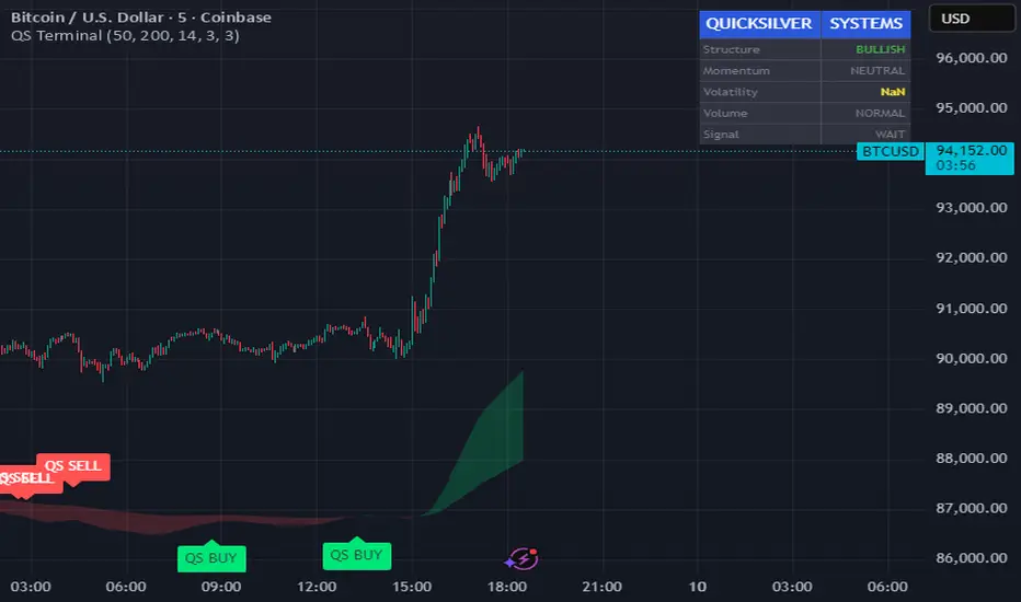
Quicksilver Master Terminal [Institutional]Overview
The Quicksilver Master Terminal is a comprehensive data visualization interface designed to bring institutional-grade market awareness to the retail chart. It replaces the need for multiple cluttered indicators by consolidating Trend, Momentum, Volatility, and Structure into a single Heads-Up Display (HUD).
Designed by Quicksilver Algo Systems, this tool is engineered for precision scalpers and prop firm traders who require instant situational awareness without switching timeframes.
Features
1. The Institutional HUD (Heads-Up Display)
Located in the top-right corner, this live dashboard provides real-time metrics on:
Market Structure: Instantly identifies if the asset is in a Bullish or Bearish regime relative to the 200 EMA.
Momentum Status: Tracks overbought/oversold conditions using smoothed Stochastic logic.
Volatility (ATR): Displays live Average True Range data for precise Stop Loss placement.
Volume Flow: Detects institutional volume spikes (1.5x average).
2. The Trend Cloud
A dynamic visual ribbon that fills the space between the Fast EMA (50) and Slow EMA (200).
Green Cloud: Strong Bullish Trend (Look for Longs).
Red Cloud: Strong Bearish Trend (Look for Shorts).
Cross: Visual warning of trend reversals.
3. Sniper Signal Logic
The script paints "INSTITUTIONAL BUY" and "INSTITUTIONAL SELL" labels only when high-probability confluence occurs:
Exhaustion: Stochastic RSI breaches extreme levels (<20 or >80).
Confirmation: Price action aligns with Heikin Ashi smoothing to filter noise.
Momentum: Fast %K crosses Slow %D.
How to Use
For Scalping (1m - 5m): Wait for the Trend Cloud to align with the Signal. Take "BUY" signals only when the Cloud is Green.
For Risk Management: Use the live "Volatility" number in the HUD to set your Stop Loss (e.g., 1.5x the current Volatility value).
About the Developer
This script is part of the Quicksilver Ecosystem. We build algorithmic solutions focused on capital preservation and risk management for funded traders.
Disclaimer: This tool is for educational market analysis only. Past performance is not indicative of future results.
Macros+AMD [NW]Macros + AMD - Daily & Weekly Time-Based Analysis
Multi-timeframe AMD (Accumulation, Manipulation, Distribution) visualization with ICT Macro timing windows for time-based market analysis.
Overview
This indicator visualizes the AMD (Accumulation, Manipulation, Distribution) framework on both daily and weekly timeframes, combined with ICT Macro timing windows. It is designed as an educational tool to help traders study time-based market structure and algorithmic price delivery concepts.
The AMD model is based on the idea that markets move through distinct phases within each trading period:
Accumulation (A) - Initial range formation, liquidity building
Manipulation (M) - False moves to trap traders, liquidity sweeps
Distribution (D) - True directional move, price delivery to targets
What This Indicator Displays
Daily AMD Phases
Displays the intraday AMD cycle based on New York trading hours:
A Phase (Blue): 4:00 AM - 8:35 AM EST — Morning accumulation, Asian/London overlap
M Phase (Red): 8:35 AM - 11:25 AM EST — NY session manipulation, news events
D Phase (Green): 11:25 AM - 4:00 PM EST — Afternoon distribution and price delivery
Weekly AMD Phases
Displays the weekly AMD cycle from Monday to Monday:
A Phase: Monday 00:00 - Tuesday 21:56 EST — Weekly high/low formation begins
M Phase: Tuesday 21:56 - Thursday 02:04 EST — Mid-week reversal zone
D Phase: Thursday 02:04 - Monday 00:00 EST — Weekly price delivery
Inner M Phase Fibs
When enabled, subdivides the M (Manipulation) phase using Fibonacci levels:
0.382 level — Inner accumulation ends
0.500 level — Mid-point of manipulation
0.618 level — Inner distribution begins
This helps identify potential reversal points within the manipulation phase.
ICT Macro Windows
Horizontal lines marking the XX:42 to XX:15 macro periods (33-minute windows):
2:42 - 3:15 AM
3:42 - 4:15 AM (London)
7:42 - 8:15 AM
8:42 - 9:15 AM
9:42 - 10:15 AM (Prime AM session)
10:42 - 11:15 AM
11:42 - 12:15 PM
12:42 - 1:15 PM
1:42 - 2:15 PM
2:42 - 3:15 PM
These windows represent times when algorithmic price delivery is more likely to occur.
How To Use
Understanding the AMD Framework
During the A Phase:
Observe range formation and initial liquidity pools
Note the high and low established during this phase
Wait for manipulation before committing to direction
During the M Phase:
Watch for false breakouts and stop hunts
Look for reversal patterns after liquidity sweeps
The inner fibs (0.382, 0.5, 0.618) can help time entries within this phase
Mid-week (Wednesday) often sees key reversals on weekly AMD
During the D Phase:
This is typically when the true move occurs
Price tends to deliver toward draw on liquidity targets
The direction is often opposite to the manipulation move
Using the Macro Windows
The XX:42 to XX:15 windows are times to pay attention to price action:
These 33-minute periods often see increased algorithmic activity
Look for displacement, fair value gaps, or order blocks forming
The 9:42-10:15 AM window is considered particularly significant for NY session
Weekly Day Labels
Monday/Tuesday: "H/L of Week" — Watch for weekly high or low formation
Wednesday: "Reversal Day" — Mid-week reversal probability increases
Thursday/Friday: "Reversal Day" — Continuation or secondary reversal
Settings Guide
Main Settings
Timezone: Set to your broker's timezone or preferred timezone
Macros On Top: Toggle macro lines above or below AMD boxes
Show All Text Labels: Master toggle for all text (turn off for clean charts on HTF)
Daily/Weekly AMD
Show: Enable/disable the AMD visualization
Opacity: Adjust transparency of the phase boxes (higher = more transparent)
AMD Colors
Customize colors for each phase (A, M, D)
Default: Blue (A), Red (M), Green (D)
Inner M Style
Customize the inner M phase fib lines and text colors
Default: Black lines for clean visibility
Macro Settings
Adjust macro line color and thickness
Toggle individual macro windows on/off
Important Notes
This indicator is for educational purposes and time-based analysis
It does not provide buy/sell signals
Always use in conjunction with proper price action analysis
Past price behavior during these time windows does not guarantee future results
The AMD framework is one lens for viewing market structure — use it as part of a complete methodology
Credits
This indicator is based on concepts taught by ICT (Inner Circle Trader) and the broader Smart Money Concepts community. The AMD framework, macro timing windows, and weekly profile concepts are derived from this educational methodology.
Timeframe Recommendations
Best viewed on 1-minute to 15-minute charts
Text labels automatically hide on 9-minute and higher timeframes for cleaner visualization
Indicator hides completely on 1-hour and higher timeframes
Changelog
v1.0 - Initial release
Daily AMD phases (4am-4pm EST)
Weekly AMD phases (Monday-Monday)
Inner M phase Fibonacci subdivisions
10 ICT Macro timing windows
Full customization options
Automatic 9-day cleanup

Bitgak [Osprey]🟠 INTRODUCTION
Bitgak , translated as "Oblique Angle" in Korean, is a strategy used by multi-hundred-million traders in Korea, sometimes more heavily than Fibonacci retracement.
It is a concept that by connecting two or more pivot points on the chart and creating equidistant parallel lines, we can spot other pivot points. As seen in the example, a line at a different height but with the same angle spots many pivot points.
This indicator spots pivot points on the chart and tests all different possible Bitgak lines with a brute-force method. Then it shows the parallel line configuration with the most pivots hitting it. You may use the lines drawn on the chart as possible reversal points.
It is best to use on Day and Week candles . In the very short range of time, the noise makes it hard to capture meaningful data.
🟠 HOW TO USE
The orange dots are the major pivot points (you can set the period of the long-term pivot) upon which the lines are built.
Change the "Manual Lookback Bars" from 300 to a meaningful period upon your inspection.
"Hit Tolerance %" means how close a pivot needs to be to the line to be considered as having touched the line.
If the line is too narrow, which is not very useful, you may consider increasing the "Long-term Pivot Bars" and experimenting with different settings for Channel Lines and Heuristics.
The result:
"Top Anchors to Test (L)" is how many L highest peaks and L lowest troughs should be weighed heavily when testing the lines. That is, with L = 1, the algorithm will reward the Bitgak lines that touch 1 highest peak and 1 lowest trough. It doesn't make much intuitive sense, so I suggest just testing it out.
🟠 HOW IT WORKS
Step 1: Pivot Detection
The indicator runs two parallel detection systems:
Short-term pivots (default: 7 bars on each side) - Captures minor swing highs/lows for detailed analysis
Long-term pivots (default: 17 bars on each side) - Identifies major structural turning points
These pivots form the foundation for all channel calculations.
Step 2: Anchor Point Selection
From the detected long-term pivots, the algorithm identifies:
The L highest peaks (default L=1, meaning the single highest peak)
The L lowest troughs (default L=1, meaning the single lowest trough)
These become potential "anchor points" for channel construction. Higher L values test more combinations but increase computation time.
Step 3: Channel Candidate Generation
For support channels: Every pair of troughs becomes a potential base line (A-B)
For resistance channels: Every pair of peaks becomes a potential base line (A-B)
The algorithm then tests each peak (for support) or trough (for resistance) as pivot C.
Step 4: Optimal Spacing Calculation
For each A-B-C combination, the algorithm calculates:
Unit Spacing = (Distance from C to A-B line) / Multiplier
It tests multipliers from 0.5 to 4.0 (or your custom range), asking: "If pivot C sits on the 1.0 line, what spacing makes the most pivots hit other lines?"
Step 5: Scoring & Selection
Each configuration is scored by counting how many pivots fall within tolerance (default 1% of price) of any parallel line in the range . The highest-scoring channel is drawn on your chart.

Simplified Percentile ClusteringSimplified Percentile Clustering (SPC) is a clustering system for trend regime analysis.
Instead of relying on heavy iterative algorithms such as k-means, SPC takes a deterministic approach: it uses percentiles and running averages to form cluster centers directly from the data, producing smooth, interpretable market state segmentation that updates live with every bar.
Most clustering algorithms are designed for offline datasets, they require recomputation, multiple iterations, and fixed sample sizes.
SPC borrows from both statistical normalization and distance-based clustering theory , but simplifies them. Percentiles ensure that cluster centers are resistant to outliers , while the running mean provides a stable mid-point reference.
Unlike iterative methods, SPC’s centers evolve smoothly with time, ideal for charts that must update in real time without sudden reclassification noise.
SPC provides a simple yet powerful clustering heuristic that:
Runs continuously in a charting environment,
Remains interpretable and reproducible,
And allows traders to see how close the current market state is to transitioning between regimes.
Clustering by Percentiles
Traditional clustering methods find centers through iteration. SPC defines them deterministically using three simple statistics within a moving window:
Lower percentile (p_low) → captures the lower basin of feature values.
Upper percentile (p_high) → captures the upper basin.
Mean (mid) → represents the central tendency.
From these, SPC computes stable “centers”:
// K = 2 → two regimes (e.g., bullish / bearish)
=
// K = 3 → adds a neutral zone
=
These centers move gradually with the market, forming live regime boundaries without ever needing convergence steps.
Two clusters capture directional bias; three clusters add a neutral ‘range’ state.
Multi-Feature Fusion
While SPC can cluster a single feature such as RSI, CCI, Fisher Transform, DMI, Z-Score, or the price-to-MA ratio (MAR), its real strength lies in feature fusion. Each feature adds a unique lens to the clustering system. By toggling features on or off, traders can test how each dimension contributes to the regime structure.
In “Clusters” mode, SPC measures how far the current bar is from each cluster center across all enabled features, averages these distances, and assigns the bar to the nearest combined center. This effectively creates a multi-dimensional regime map , where each feature contributes equally to defining the overall market state.
The fusion distance is computed as:
dist := (rsi_d * on_off(use_rsi) + cci_d * on_off(use_cci) + fis_d * on_off(use_fis) + dmi_d * on_off(use_dmi) + zsc_d * on_off(use_zsc) + mar_d * on_off(use_mar)) / (on_off(use_rsi) + on_off(use_cci) + on_off(use_fis) + on_off(use_dmi) + on_off(use_zsc) + on_off(use_mar))
Because each feature can be standardized (Z-Score), the distances remain comparable across different scales.
Fusion mode combines multiple standardized features into a single smooth regime signal.
Visualizing Proximity - The Transition Gradient
Most indicators show binary or discrete conditions (e.g., bullish/bearish). SPC goes further, it quantifies how close the current value is to flipping into the next cluster.
It measures the distances to the two nearest cluster centers and interpolates between them:
rel_pos = min_dist / (min_dist + second_min_dist)
real_clust = cluster_val + (second_val - cluster_val) * rel_pos
This real_clust output forms a continuous line that moves smoothly between clusters:
Near 0.0 → firmly within the current regime
Around 0.5 → balanced between clusters (transition zone)
Near 1.0 → about to flip into the next regime
Smooth interpolation reveals when the market is close to a regime change.
How to Tune the Parameters
SPC includes intuitive parameters to adapt sensitivity and stability:
K Clusters (2–3): Defines the number of regimes. K = 2 for trend/range distinction, K = 3 for trend/neutral transitions.
Lookback: Determines the number of past bars used for percentile and mean calculations. Higher = smoother, more stable clusters. Lower = faster reaction to new trends.
Lower / Upper Percentiles: Define what counts as “low” and “high” states. Adjust to widen or tighten cluster ranges.
Shorter lookbacks react quickly to shifts; longer lookbacks smooth the clusters.
Visual Interpretation
In “Clusters” mode, SPC plots:
A colored histogram for each cluster (red, orange, green depending on K)
Horizontal guide lines separating cluster levels
Smooth proximity transitions between states
Each bar’s color also changes based on its assigned cluster, allowing quick recognition of when the market transitions between regimes.
Cluster bands visualize regime structure and transitions at a glance.
Practical Applications
Identify market regimes (bullish, neutral, bearish) in real time
Detect early transition phases before a trend flip occurs
Fuse multiple indicators into a single consistent signal
Engineer interpretable features for machine-learning research
Build adaptive filters or hybrid signals based on cluster proximity
Final Notes
Simplified Percentile Clustering (SPC) provides a balance between mathematical rigor and visual intuition. It replaces complex iterative algorithms with a clear, deterministic logic that any trader can understand, and yet retains the multidimensional insight of a fusion-based clustering system.
Use SPC to study how different indicators align, how regimes evolve, and how transitions emerge in real time. It’s not about predicting; it’s about seeing the structure of the market unfold.
Disclaimer
This indicator is intended for educational and analytical use.
It does not generate buy or sell signals.
Historical regime transitions are not indicative of future performance.
Always validate insights with independent analysis before making trading decisions.

Advanced Speedometer Gauge [PhenLabs]Advanced Speedometer Gauge
Version: PineScript™v6
📌 Description
The Advanced Speedometer Gauge is a revolutionary multi-metric visualization tool that consolidates 13 distinct trading indicators into a single, intuitive speedometer display. Instead of cluttering your workspace with multiple oscillators and panels, this gauge provides a unified interface where you can switch between different metrics while maintaining consistent visual interpretation.
Built on PineScript™ v6, the indicator transforms complex technical calculations into an easy-to-read semi-circular gauge with color-coded zones and a precision needle indicator. Each of the 13 available metrics has been carefully normalized to a 0-100 scale, ensuring that whether you’re analyzing RSI, volume trends, or volatility extremes, the visual interpretation remains consistent and intuitive.
The gauge is designed for traders who value efficiency and clarity. By consolidating multiple analytical perspectives into one compact display, you can quickly assess market conditions without the visual noise of traditional multi-indicator setups. All metrics are non-overlapping, meaning each provides unique insights into different aspects of market behavior.
🚀 Points of Innovation
13 selectable metrics covering momentum, volume, volatility, trend, and statistical analysis, all accessible through a single dropdown menu
Universal 0-100 normalization system that standardizes different indicator scales for consistent visual interpretation across all metrics
Semi-circular gauge design with 21 arc segments providing smooth precision and clear visual feedback through color-coded zones
Non-redundant metric selection ensuring each indicator provides unique market insights without analytical overlap
Advanced metrics including MFI (volume-weighted momentum), CCI (statistical deviation), Volatility Rank (extended lookback), Trend Strength (ADX-style), Choppiness Index, Volume Trend, and Price Distance from MA
Flexible positioning system with 5 chart locations, 3 size options, and fully customizable color schemes for optimal workspace integration
🔧 Core Components
Metric Selection Engine: Dropdown interface allowing instant switching between 13 different technical indicators, each with independent parameter controls
Normalization System: All metrics converted to 0-100 scale using indicator-specific algorithms that preserve the statistical significance of each measurement
Semi-Circular Gauge: Visual display using 21 arc segments arranged in curved formation with two-row thickness for enhanced visibility
Color Zone System: Three distinct zones (0-40 green, 40-70 yellow, 70-100 red) providing instant visual feedback on metric extremes
Needle Indicator: Dynamic pointer that positions across the gauge arc based on precise current metric value
Table Implementation: Professional table structure ensuring consistent positioning and rendering across different chart configurations
🔥 Key Features
RSI (Relative Strength Index): Classic momentum oscillator measuring overbought/oversold conditions with adjustable period length (default 14)
Stochastic Oscillator: Compares closing price to price range over specified period with smoothing, ideal for identifying momentum shifts
MFI (Money Flow Index): Volume-weighted RSI that combines price movement with volume to measure buying and selling pressure intensity
CCI (Commodity Channel Index): Measures statistical deviation from average price, normalized from typical -200 to +200 range to 0-100 scale
Williams %R: Alternative overbought/oversold indicator using high-low range analysis, inverted to match 0-100 scale conventions
Volume %: Current volume relative to moving average expressed as percentage, capped at 100 for extreme spikes
Volume Trend: Cumulative directional volume flow showing whether volume is flowing into up moves or down moves over specified period
ATR Percentile: Current Average True Range position within historical range using specified lookback period (default 100 bars)
Volatility Rank: Close-to-close volatility measured against extended historical range (default 252 days), differs from ATR in calculation method
Momentum: Rate of change calculation showing price movement speed, centered at 50 and normalized to 0-100 range
Trend Strength: ADX-style calculation using directional movement to quantify trend intensity regardless of direction
Choppiness Index: Measures market choppiness versus trending behavior, where high values indicate ranging markets and low values indicate strong trends
Price Distance from MA: Measures current price over-extension from moving average using standard deviation calculations
🎨 Visualization
Semi-Circular Arc Display: Curved gauge spanning from 0 (left) to 100 (right) with smooth progression and two-row thickness for visibility
Color-Coded Zones: Green zone (0-40) for low/oversold conditions, yellow zone (40-70) for neutral readings, red zone (70-100) for high/overbought conditions
Needle Indicator: Downward-pointing triangle (▼) positioned precisely at current metric value along the gauge arc
Scale Markers: Vertical line markers at 0, 25, 50, 75, and 100 positions with corresponding numerical labels below
Title Display: Merged cell showing “𓄀 PhenLabs” branding plus currently selected metric name in monospace font
Large Value Display: Current metric value shown with two decimal precision in large text directly below title
Table Structure: Professional table with customizable background color, text color, and transparency for minimal chart obstruction
📖 Usage Guidelines
Metric Selection
Select Metric: Default: RSI | Options: RSI, Stochastic, Volume %, ATR Percentile, Momentum, MFI (Money Flow), CCI (Commodity Channel), Williams %R, Volatility Rank, Trend Strength, Choppiness Index, Volume Trend, Price Distance | Choose the technical indicator you want to display on the gauge based on your current analytical needs
RSI Settings
RSI Length: Default: 14 | Range: 1+ | Controls the lookback period for RSI calculation, shorter periods increase sensitivity to recent price changes
Stochastic Settings
Stochastic Length: Default: 14 | Range: 1+ | Lookback period for stochastic calculation comparing close to high-low range
Stochastic Smooth: Default: 3 | Range: 1+ | Smoothing period applied to raw stochastic value to reduce noise and false signals
Volume Settings
Volume MA Length: Default: 20 | Range: 1+ | Moving average period used to calculate average volume for comparison with current volume
Volume Trend Length: Default: 20 | Range: 5+ | Period for calculating cumulative directional volume flow trend
ATR and Volatility Settings
ATR Length: Default: 14 | Range: 1+ | Period for Average True Range calculation used in ATR Percentile metric
ATR Percentile Lookback: Default: 100 | Range: 20+ | Historical range used to determine current ATR position as percentile
Volatility Rank Lookback (Days): Default: 252 | Range: 50+ | Extended lookback period for Volatility Rank metric using close-to-close volatility
Momentum and Trend Settings
Momentum Length: Default: 10 | Range: 1+ | Lookback period for rate of change calculation in Momentum metric
Trend Strength Length: Default: 20 | Range: 5+ | Period for directional movement calculations in ADX-style Trend Strength metric
Advanced Metric Settings
MFI Length: Default: 14 | Range: 1+ | Lookback period for Money Flow Index calculation combining price and volume
CCI Length: Default: 20 | Range: 1+ | Period for Commodity Channel Index statistical deviation calculation
Williams %R Length: Default: 14 | Range: 1+ | Lookback period for Williams %R high-low range analysis
Choppiness Index Length: Default: 14 | Range: 5+ | Period for calculating market choppiness versus trending behavior
Price Distance MA Length: Default: 50 | Range: 10+ | Moving average period used for Price Distance standard deviation calculation
Visual Customization
Position: Default: Top Right | Options: Top Left, Top Right, Bottom Left, Bottom Right, Middle Right | Controls gauge placement on chart for optimal workspace organization
Size: Default: Normal | Options: Small, Normal, Large | Adjusts overall gauge dimensions and text size for different monitor resolutions and preferences
Low Zone Color (0-40): Default: Green (#00FF00) | Customize color for low/oversold zone of gauge arc
Medium Zone Color (40-70): Default: Yellow (#FFFF00) | Customize color for neutral/medium zone of gauge arc
High Zone Color (70-100): Default: Red (#FF0000) | Customize color for high/overbought zone of gauge arc
Background Color: Default: Semi-transparent dark gray | Customize gauge background for contrast and chart integration
Text Color: Default: White (#FFFFFF) | Customize all text elements including title, value, and scale labels
✅ Best Use Cases
Quick visual assessment of market conditions when you need instant feedback on whether an asset is in extreme territory across multiple analytical dimensions
Workspace organization for traders who monitor multiple indicators but want to reduce chart clutter and visual complexity
Metric comparison by switching between different indicators while maintaining consistent visual interpretation through the 0-100 normalization
Overbought/oversold identification using RSI, Stochastic, Williams %R, or MFI depending on whether you prefer price-only or volume-weighted analysis
Volume analysis through Volume %, Volume Trend, or MFI to confirm price movements with corresponding volume characteristics
Volatility monitoring using ATR Percentile or Volatility Rank to identify expansion/contraction cycles and adjust position sizing
Trend vs range identification by comparing Trend Strength (high values = trending) against Choppiness Index (high values = ranging)
Statistical over-extension detection using CCI or Price Distance to identify when price has deviated significantly from normal behavior
Multi-timeframe analysis by duplicating the gauge on different timeframe charts to compare metric readings across time horizons
Educational purposes for new traders learning to interpret technical indicators through consistent visual representation
⚠️ Limitations
The gauge displays only one metric at a time, requiring manual switching to compare different indicators rather than simultaneous multi-metric viewing
The 0-100 normalization, while providing consistency, may obscure the raw values and specific nuances of each underlying indicator
Table-based visualization cannot be exported or saved as an image separately from the full chart screenshot
Optimal parameter settings vary by asset type, timeframe, and market conditions, requiring user experimentation for best results
💡 What Makes This Unique
Unified Multi-Metric Interface: The only gauge-style indicator offering 13 distinct metrics through a single interface, eliminating the need for multiple oscillator panels
Non-Overlapping Analytics: Each metric provides genuinely unique insights—MFI combines volume with price, CCI measures statistical deviation, Volatility Rank uses extended lookback, Trend Strength quantifies directional movement, and Choppiness Index measures ranging behavior
Universal Normalization System: All metrics standardized to 0-100 scale using indicator-appropriate algorithms that preserve statistical meaning while enabling consistent visual interpretation
Professional Visual Design: Semi-circular gauge with 21 arc segments, precision needle positioning, color-coded zones, and clean table implementation that maintains clarity across all chart configurations
Extensive Customization: Independent parameter controls for each metric, five position options, three size presets, and full color customization for seamless workspace integration
🔬 How It Works
1. Metric Calculation Phase:
All 13 metrics are calculated simultaneously on every bar using their respective algorithms with user-defined parameters
Each metric applies its own specific calculation method—RSI uses average gains vs losses, Stochastic compares close to high-low range, MFI incorporates typical price and volume, CCI measures deviation from statistical mean, ATR calculates true range, directional indicators measure up/down movement, and statistical metrics analyze price relationships
2. Normalization Process:
Each calculated metric is converted to a standardized 0-100 scale using indicator-appropriate transformations
Some metrics are naturally 0-100 (RSI, Stochastic, MFI, Williams %R), while others require scaling—CCI transforms from ±200 range, Momentum centers around 50, Volume ratio caps at 2x for 100, ATR and Volatility Rank calculate percentile positions, and Price Distance scales by standard deviations
3. Gauge Rendering:
The selected metric’s normalized value determines the needle position across 21 arc segments spanning 0-100
Each arc segment receives its color based on position—segments 0-8 are green zone, segments 9-14 are yellow zone, segments 15-20 are red zone
The needle indicator (▼) appears in row 5 at the column corresponding to the current metric value, providing precise visual feedback
4. Table Construction:
The gauge uses TradingView’s table system with merged cells for title and value display, ensuring consistent positioning regardless of chart configuration
Rows are allocated as follows: Row 0 merged for title, Row 1 merged for large value display, Row 2 for spacing, Rows 3-4 for the semi-circular arc with curved shaping, Row 5 for needle indicator, Row 6 for scale markers, Row 7 for numerical labels at 0/25/50/75/100
All visual elements update on every bar when barstate.islast is true, ensuring real-time accuracy without performance impact
💡 Note:
This indicator is designed for visual analysis and market condition assessment, not as a standalone trading system. For best results, combine gauge readings with price action analysis, support and resistance levels, and broader market context. Parameter optimization is recommended based on your specific trading timeframe and asset class. The gauge works on all timeframes but may require different parameter settings for intraday versus daily/weekly analysis. Consider using multiple instances of the gauge set to different metrics for comprehensive market analysis without switching between settings.

Smart Money Support/Resistance - LiteSmart Money Support/Resistance — Lite
Overview & Methodology
This indicator identifies support and resistance as zones derived from concentrated buying and selling pressure, rather than relying solely on traditional swing highs/lows. Its design focuses on transparency: how data is sourced, how zones are computed, and how the on‑chart display should be interpreted.
Lower‑Timeframe (LTF) Data
The script requests Up Volume, Down Volume, and Volume Delta from a lower timeframe to expose intrabar order‑flow structure that the chart’s native timeframe cannot show. In practical terms, this lets you see where buyers or sellers briefly dominated inside the body of a higher‑timeframe bar.
bool use_custom_tf_input = input.bool(true, title="Use custom lower timeframe", tooltip="Override the automatically chosen lower timeframe for volume calculations.", group=grpVolume)
string custom_tf_input = input. Timeframe("1", title="Lower timeframe", tooltip="Lower timeframe used for up/down volume calculations (default 5 seconds).", group=grpVolume)
import TradingView/ta/10 as tvta
resolve_lower_tf(useCustom, customTF) =>
useCustom ? customTF :
timeframe.isseconds ? "1S" :
timeframe.isintraday ? "1" :
timeframe.isdaily ? "5" : "60"
get_up_down_volume(lowerTf) =>
= tvta.requestUpAndDownVolume(lowerTf)
var float upVolume = na
var float downVolume = na
var float deltaVolume = na
string lower_tf = resolve_lower_tf(use_custom_tf_input, custom_tf_input)
= get_up_down_volume(lower_tf)
upVolume := u_tmp
downVolume := d_tmp
deltaVolume := dl_tmp
• Data source: TradingView’s ta.requestUpAndDownVolume(lowerTf) via the official TA library.
• Plan capabilities: higher‑tier subscriptions unlock seconds‑based charts and allow more historical bars per chart. This expands both the temporal depth of LTF data and the precision of short‑horizon analysis, while base tiers provide minute‑level data suitable for day/short‑swing studies.
• Coverage clarity: a small on‑chart Coverage Panel reports the active lower timeframe, the number of bars covered, and the latest computed support/resistance ranges so you always know the bounds of valid LTF input.
Core Method
1) Data acquisition (LTF)
The script retrieves three series from the chosen lower timeframe:
– Up Volume (buyers)
– Down Volume (sellers)
– Delta (Up – Down)
2) Rolling window & extrema
Over a user‑defined lookback (Global Volume Period), the algorithm builds rolling arrays of completed bars and scans for extrema:
– Buyers_max / Buyers_min from Up Volume
– Sellers_max / Sellers_min from Down Volume
Only completed bars are considered; the current bar is excluded for stability.
3) Price mapping
The extrema are mapped back to their source candles to obtain price bounds:
– For “maximum” roles the algorithm uses the relevant candle highs.
– For “minimum” roles it uses the relevant candle lows.
These pairs define candidate resistance (max‑based) and support (min‑based) zones or vice versa.
4) Zone construction & minimum width
To ensure practicality on all symbols, zones enforce a minimum vertical thickness of two ticks. This prevents visually invisible or overly thin ranges on instruments with tight ticks.
5) Vertical role resolution
When both max‑ and min‑based zones exist, the script compares their midpoints. If, due to local price structure, the min‑based zone sits above the max‑based zone, display roles are swapped so the higher zone is labeled Resistance and the lower zone Support. Colors/widths are updated accordingly to keep the visual legend consistent.
6) Rendering & panel
Two horizontal lines and a filled box represent each active zone. The Coverage Panel (bottom‑right by default) prints:
– Lower‑timeframe in use
– Number of bars covered by LTF data
– Current Support and Resistance ranges
If the two zones overlap, an additional “Range Market” note is shown.
Key Inputs
• Global Volume Period: shared lookback window for the extrema search.
• Lower timeframe: user‑selectable override of the automatically resolved lower timeframe.
• Visualization toggles: independent show/hide controls and colors for maximum (resistance) and minimum (support) zones.
• Coverage Panel: enable/disable the single‑cell table and its readout.
Operational Notes
• The algorithm aligns all lookups to completed bars (no peeking). Price references are shifted appropriately to avoid using the still‑forming bar in calculations.
• Second‑based lower timeframes improve granularity for scalping and very short‑term entries. Minute‑based lower timeframes provide broader coverage for intraday and short‑swing contexts.
• Use the Coverage Panel to confirm the true extent of available LTF history on your symbol/plan before drawing conclusions from very deep lookbacks.
Visual Walkthrough
A step‑by‑step image sequence accompanies this description. Each figure demonstrates how the indicator reads LTF volume, locates extrema, builds price‑mapped zones, and updates labels/colors when vertical order requires it.
Chart Interpretation
This chart illustrates two distinct perspectives of the Smart Money Support/Resistance — Lite indicator, each derived from different lookback horizons and lower-timeframe (LTF) resolutions.
1- Short-term view (43 bars, 10-second LTF)
Using the most recent 43 completed bars with 10-second intrabar data, the algorithm detects that both maximum and minimum volume extrema fall within a narrow range. The result is a clearly identified range market: resistance between 178.15–184.55 and support between 175.02–179.38.
The Coverage Panel (bottom-right) confirms the scope of valid input: the lower timeframe used, number of bars covered, and the resulting zones. This short-term scan highlights how the indicator adapts to limited data depth, flagging sideways structure where neither side dominates.
2 - Long-term view (120 bars, 30-second LTF)
Over a wider 120-bar lookback with higher-granularity 30-second data, broader supply and demand zones emerge.
– The long-term resistance zone captures the concentration of buyers and sellers at the upper boundary of recent price history.
– The long-term support zone anchors to the opposite side of the distribution, derived from maxima and minima of both buying and selling pressure.
These zones reflect deeper structural levels where market participants previously committed significant volume.
Combined Perspective
By aligning the short-term and long-term outputs, the chart shows how the indicator distinguishes immediate consolidation (range market) from more durable support and resistance levels derived from extended history. This dual resolution approach makes clear that support and resistance are not static lines but dynamic zones, dependent on both timeframe depth and the resolution of intrabar volume data.

Lorentzian Key Support and Resistance Level Detector [mishy]🧮 Lorentzian Key S/R Levels Detector
Advanced Support & Resistance Detection Using Mathematical Clustering
The Problem
Traditional S/R indicators fail because they're either subjective (manual lines), rigid (fixed pivots), or break when price spikes occur. Most importantly, they don't tell you where prices actually spend time, just where they touched briefly.
The Solution: Lorentzian Distance Clustering
This indicator introduces a novel approach by using Lorentzian distance instead of traditional Euclidean distance for clustering. This is groundbreaking for financial data analysis.
Data Points Clustering:
🔬 Why Euclidean Distance Fails in Trading
Traditional K-means uses Euclidean distance:
• Formula: distance = (price_A - price_B)²
• Problem: Squaring amplifies differences exponentially
• Real impact: One 5% price spike has 25x more influence than a 1% move
• Result: Clusters get pulled toward outliers, missing real support/resistance zones
Example scenario:
Prices: ← flash spike
Euclidean: Centroid gets dragged toward 150
Actual S/R zone: Around 100 (where prices actually trade)
⚡ Lorentzian Distance: The Game Changer
Our approach uses Lorentzian distance:
• Formula: distance = log(1 + (price_difference)² / σ²)
• Breakthrough: Logarithmic compression keeps outliers in check
• Real impact: Large moves still matter, but don't dominate
• Result: Clusters focus on where prices actually spend time
Same example with Lorentzian:
Prices: ← flash spike
Lorentzian: Centroid stays near 100 (real trading zone)
Outlier (150): Acknowledged but not dominant
🧠 Adaptive Intelligence
The σ parameter isn't fixed,it's calculated from market disturbance/entropy:
• High volatility: σ increases, making algorithm more tolerant of large moves
• Low volatility: σ decreases, making algorithm more sensitive to small changes
• Self-calibrating: Adapts to any instrument or market condition automatically
Why this matters: Traditional methods treat a 2% move the same whether it's in a calm or volatile market. Lorentzian adapts the sensitivity based on current market behavior.
🎯 Automatic K-Selection (Elbow Method)
Instead of guessing how many S/R levels to draw, the indicator:
• Tests 2-6 clusters and calculates WCSS (tightness measure)
• Finds the "elbow" - where adding more clusters stops helping much
• Uses sharpness calculation to pick the optimal number automatically
Result: Perfect balance between detail and clarity.
How It Works
1. Collect recent closing prices
2. Calculate entropy to adapt to current market volatility
3. Cluster prices using Lorentzian K-means algorithm
4. Auto-select optimal cluster count via statistical analysis
5. Draw levels at cluster centers with deviation bands
📊 Manual K-Selection Guide (Using WCSS & Sharpness Analysis)
When you disable auto-selection, use both WCSS and Sharpness metrics from the analysis table to choose manually:
What WCSS tells you:
• Lower WCSS = tighter clusters = better S/R levels
• Higher WCSS = scattered clusters = weaker levels
What Sharpness tells you:
• Higher positive values = optimal elbow point = best K choice
• Lower/negative values = poor elbow definition = avoid this K
• Measures the "sharpness" of the WCSS curve drop-off
Decision strategy using both metrics:
K=2: WCSS = 150.42 | Sharpness = - | Selected =
K=3: WCSS = 89.15 | Sharpness = 22.04 | Selected = ✓ ← Best choice
K=4: WCSS = 76.23 | Sharpness = 1.89 | Selected =
K=5: WCSS = 73.91 | Sharpness = 1.43 | Selected =
Quick decision rules:
• Pick K with highest positive Sharpness (indicates optimal elbow)
• Confirm with significant WCSS drop (30%+ reduction is good)
• Avoid K values with negative or very low Sharpness (<1.0)
• K=3 above shows: Big WCSS drop (41%) + High Sharpness (22.04) = Perfect choice
Why this works:
The algorithm finds the "elbow" where adding more clusters stops being useful. High Sharpness pinpoints this elbow mathematically, while WCSS confirms the clustering quality.
Elbow Method Visualization:
Traditional clustering problems:
❌ Price spikes distort results
❌ Fixed parameters don't adapt
❌ Manual tuning is subjective
❌ No way to validate choices
Lorentzian solution:
☑️ Outlier-resistant distance metric
☑️ Entropy-based adaptation to volatility
☑️ Automatic optimal K selection
☑️ Statistical validation via WCSS & Sharpness
Features
Visual:
• Color-coded levels (red=highest resistance, green=lowest support)
• Optional deviation bands showing cluster spread
• Strength scores on labels: Each cluster shows a reliability score.
• Higher scores (0.8+) = very strong S/R levels with tight price clustering
• Lower scores (0.6-0.7) = weaker levels, use with caution
• Based on cluster tightness and data point density
• Clean line extensions and labels
Analytics:
• WCSS analysis table showing why K was chosen
• Cluster metrics and statistics
• Real-time entropy monitoring
Control:
• Auto/manual K selection toggle
• Customizable sample size (20-500 bars)
• Show/hide bands and metrics tables
The Result
You get mathematically validated S/R levels that focus on where prices actually cluster, not where they randomly spiked. The algorithm adapts to market conditions and removes guesswork from level selection.
Best for: Traders who want objective, data-driven S/R levels without manual chart analysis.
Credits: This script is for educational purposes and is inspired by the work of @ThinkLogicAI and an amazing mentor @DskyzInvestments . It demonstrates how Lorentzian geometrical concepts can be applied not only in ML classification but also quite elegantly in clustering.

GTrader-ICT All In One-Comumnity VersionMeet the **GTrader-ICT All In One **, a comprehensive toolkit designed to integrate key Inner Circle Trader (ICT) concepts directly onto your chart. This powerful overlay indicator consolidates multiple essential tools, streamlining your technical analysis and helping you identify key temporal and price-based events.
📚 References & Inspiration
This indicator stands on the shoulders of giants. With the help of **tradeforopp** and **LuxAlgo**. The concepts and some implementation details were referenced from the following excellent, publicly available scripts:
ICT Killzones: The session drawing and pivot logic is adapted from tradeforopp
ICT Macros: The macro detection and plotting functionality is inspired by the work of Lux Algo , particularly their widely-used indicators covering ICT concepts.
🎯 Core Features
* **ICT Killzones:** Visualize critical trading sessions with customizable boxes. You can easily toggle and style the **Asia**, **London**, and **New York (AM, Lunch, PM)** sessions to focus on the liquidity and volatility that matter most to your strategy.
* Fully customizable session times and colors.
* Timezone support to align sessions with your local or preferred trading time (defaults to `America/New_York`).
* **ICT Macros:** Automatically identify and plot specific, short-duration time windows where institutional algorithms are known to be active (e.g., `09:50-10:10`, `14:50-15:10`, etc.).
* Plots the high/low range of the macro, providing clear levels of interest.
* Utilizes 1-minute data for precision, even when viewing on 3-minute or 5-minute charts.
📚 Optimization over the other original indicators
We add the custom input for macros session, users just need to input the from/to hour: minute format, and they will be converted into session objects in pinescript
The macro draws function is optimized, removing redundant draws, leading to better performance
Add "Distance from Macro Line to Chart" option
Add "Session Drawings Limit" for better performance
⚠️ Notes on TradingView Warnings
You may encounter some warnings from TradingView when using this script. These are generally expected due to the script's advanced, event-driven nature:
1. **Function Call Consistency:** The function 'box.new' should be called on each calculation for consistency, which may appear. This happens because drawing elements (like session boxes) are intentionally created only on the *first bar* of a new session, not on every single bar. This is a necessary design choice for performance and to prevent duplicate drawings.
2. **Potential for Repainting/Slow Load:** The **Macro** feature uses the `request.security_lower_tf()` function to get accurate 1-minute data. This can trigger warnings about performance or slow loading times. This is a known trade-off for achieving the precision required for the feature.

Machine Learning | Adaptive Trend Signals [Bitwardex]⚙️🧠Machine Learning | Adaptive Trend Signals
🔷Overview
Machine Learning | Adaptive Trend Signals is a Pine Script™ v6 indicator designed to visualize market trends and generate signals through a combination of volatility clustering, Gaussian smoothing, and adaptive trend calculations. Built as an overlay indicator, it integrates advanced techniques inspired by machine learning concepts, such as K-Means clustering, to adapt to changing market conditions. The script is highly customizable, includes a backtesting module, and supports alert conditions, making it suitable for traders exploring trend-based strategies and developers studying volatility-driven indicator design.
🔷Functionality
The indicator performs the following core functions:
• Volatility Clustering: Uses K-Means clustering to categorize market volatility into high, medium, and low states, adjusting trend sensitivity accordingly.
• Trend Calculation: Computes adaptive trend lines (SmartTrend) based on volatility-adjusted standard deviation, smoothed RSI, and ADX filters.
• Signal Generation: Identifies potential buy and sell points through trend line crossovers and directional confirmation.
• Backtesting Module: Tracks trade outcomes based on the SmartTrend3 value, displaying win rate and total trades.
• Visualization: Plots trend lines with gradient colors and optional signal markers (bullish 🐮 and bearish 🐻).
• Alerts: Provides configurable alerts for trend shifts and volatility state changes.
🔷Technical Methodology
Volatility Clustering with K-Means
The indicator employs a K-Means clustering algorithm to classify market volatility, measured via the Average True Range (ATR), into three distinct clusters:
• Data Collection: Gathers ATR values over a user-defined training period (default: 100 bars).
• Centroid Initialization: Sets initial centroids at the highest, lowest, and midpoint ATR values within the training period.
• Iterative Clustering: Assigns ATR data points to the nearest centroid, recalculates centroid means, and repeats until convergence.
• Dynamic Adjustment: Assigns a volatility state (high, medium, or low) based on the closest centroid, adjusting the trend factor (e.g., tighter for high volatility, wider for low volatility).
This approach allows the indicator to adapt its sensitivity to varying market conditions, providing a data-driven foundation for trend calculations.
🔷Gaussian Smoothing
To enhance signal clarity and reduce noise, the indicator applies Gaussian kernel smoothing to:
• RSI: Smooths the Relative Strength Index (calculated from OHLC4) to filter short-term fluctuations.
• SmartTrend: Smooths the primary trend line for a more stable output.
The Gaussian kernel uses a sigma value derived from the user-defined smoothing length, ensuring mathematically consistent noise reduction.
🔷SmartTrend Calculation
The pineSmartTrend function is the core of the indicator, producing three trend lines:
• SmartTrend: The primary trend line, calculated using a volatility-adjusted standard deviation, smoothed RSI, and ADX conditions.
• SmartTrend2: A secondary trend line with a wider factor (base factor * 1.382) for signal confirmation.
SmartTrend3: The average of SmartTrend and SmartTrend2, used for plotting and backtesting.
Key components of the calculation include:
• Dynamic Standard Deviation: Scales based on ATR relative to its 50-period smoothed average, with multipliers (1.0 to 1.4) applied according to volatility thresholds.
• RSI and ADX Filters: Requires RSI > 50 for bullish trends or < 50 for bearish trends, alongside ADX > 15 and rising to confirm trend strength.
Volatility-Adjusted Bands: Constructs upper and lower bands around price action, adjusted by the volatility cluster’s dynamic factor.
🔷Signal Generation
The generate_signals function generates signals as follows:
• Buy Signal: Triggered when SmartTrend crosses above SmartTrend2 and the price is above SmartTrend, with directional confirmation.
• Sell Signal: Triggered when SmartTrend crosses below SmartTrend2 and the price is below SmartTrend, with directional confirmation.
Directional Logic: Tracks trend direction to filter out conflicting signals, ensuring alignment with the broader market context.
Signals are visualized as small circles with bullish (🐮) or bearish (🐻) emojis, with an option to toggle visibility.
🔷Backtesting
The get_backtest function evaluates signal outcomes using the SmartTrend3 value (rather than closing prices) to align with the trend-based methodology.
It tracks:
• Total Trades: Counts completed long and short trades.
• Win Rate: Calculates the percentage of trades where SmartTrend3 moves favorably (higher for longs, lower for shorts).
Position Management: Closes opposite positions before opening new ones, simulating a single-position trading system.
Results are displayed in a table at the top-right of the chart, showing win rate and total trades. Note that backtest results reflect the indicator’s internal logic and should not be interpreted as predictive of real-world performance.
🔷Visualization and Alerts
• Trend Lines: SmartTrend3 is plotted with gradient colors reflecting trend direction and volatility cluster, accompanied by a secondary line for visual clarity.
• Signal Markers: Optional buy/sell signals are plotted as small circles with customizable colors.
• Alerts: Supports alerts for:
• Bullish and bearish trend shifts (confirmed on bar close).
Transitions to high, medium, or low volatility states.
🔷Input Parameters
• ATR Length (default: 14): Period for ATR calculation, used in volatility clustering.
• Period (default: 21): Common period for RSI, ADX, and standard deviation calculations.
• Base SmartTrend Factor (default: 2.0): Base multiplier for volatility-adjusted bands.
• SmartTrend Smoothing Length (default: 10): Length for Gaussian smoothing of the trend line.
• Show Buy/Sell Signals? (default: true): Enables/disables signal markers.
• Bullish/Bearish Color: Customizable colors for trend lines and signals.
🔷Usage Instructions
• Apply to Chart: Add the indicator to any TradingView chart.
• Configure Inputs: Adjust parameters to align with your trading style or market conditions (e.g., shorter ATR length for faster markets).
• Interpret Output:
• Trend Lines: Use SmartTrend3’s direction and color to gauge market bias.
• Signals: Monitor bullish (🐮) and bearish (🐻) markers for potential entry/exit points.
• Backtest Table: Review win rate and total trades to understand the indicator’s behavior in historical data.
• Set Alerts: Configure alerts for trend shifts or volatility changes to support manual or automated trading workflows.
• Combine with Analysis: Use the indicator alongside other tools or market context, as it is designed to complement, not replace, comprehensive analysis.
🔷Technical Notes
• Data Requirements: Requires at least 100 bars for accurate volatility clustering. Ensure sufficient historical data is loaded.
• Market Suitability: The indicator is designed for trend detection and may perform differently in ranging or volatile markets due to its reliance on RSI and ADX filters.
• Backtesting Scope: The backtest module uses SmartTrend3 values, which may differ from price-based outcomes. Results are for informational purposes only.
• Computational Intensity: The K-Means clustering and Gaussian smoothing may increase processing time on lower timeframes or with large datasets.
🔷For Developers
The script is modular, well-commented, encouraging reuse and modification with proper attribution.
Key functions include:
• gaussianSmooth: Applies Gaussian kernel smoothing to any data series.
• pineSmartTrend: Computes adaptive trend lines with volatility and momentum filters.
• getDynamicFactor: Adjusts trend sensitivity based on volatility clusters.
• get_backtest: Evaluates signal performance using SmartTrend3.
Developers can extend these functions for custom indicators or strategies, leveraging the volatility clustering and smoothing methodologies. The K-Means implementation is particularly useful for adaptive volatility analysis.
🔷Limitations
• The indicator is not predictive and should be used as part of a broader trading strategy.
• Performance varies by market, timeframe, and parameter settings, requiring user experimentation.
• Backtest results are based on historical data and internal logic, not real-world trading conditions.
• Volatility clustering assumes sufficient historical data; incomplete data may affect accuracy.
🔷Acknowledgments
Developed by Bitwardex, inspired by machine learning concepts and adaptive trading methodologies. Community feedback is welcome via TradingView’s platform.
🔷 Risk Disclaimer
Trading involves significant risks, and most traders may incur losses. Bitwardex AI Algo is provided for informational and educational purposes only and does not constitute financial advice or a recommendation to buy or sell any financial instrument . The signals, metrics, and features are tools for analysis and do not guarantee profits or specific outcomes. Past performance is not indicative of future results. Always conduct your own due diligence and consult a financial advisor before making trading decisions.

Altcoin Reversal or Correction DetectionINDICATOR OVERVIEW: Altcoin Reversal or Correction Detection
Altcoin Reversal or Correction Detection is a powerful crypto-specific indicator designed exclusively for altcoins by analyzing their RSI values across multiple timeframes alongside Bitcoin’s RSI. Since BTC's price movements have a strong influence on altcoins, this tool helps traders better understand whether a reversal or correction signal is truly reliable or just noise. Even if an altcoin appears oversold or overbought, it may continue trending with BTC—so this indicator gives you the full picture.
The indicator is optimized for CRYPTO MARKETS only. Not suitable for BTC itself—this is a precision tool built only for ALTCOINS only.
This indicator is not only for signals but also serves as a tool for observing all the information from different timeframes of BTC and altcoins collectively.
How the Calculation Works: Algorithm Overview
The Altcoin Reversal or Correction Detection indicator relies on an algorithm that compares the RSI values of the altcoin across multiple timeframes with Bitcoin's RSI values. This allows the indicator to identify key market moments where a reversal or correction might occur.
BTC-Altcoin RSI Correlation: The algorithm looks for the correlation between Bitcoin's price movements and the altcoin's price actions, as BTC often influences the direction of altcoins. When both Bitcoin and the altcoin show either overbought or oversold conditions in a significant number of timeframes, the indicator signals the potential for a reversal or correction.
Multi-Timeframe Confirmation: Unlike traditional indicators that may focus on a single timeframe, this tool checks multiple timeframes for both BTC and the altcoin. When the same overbought/oversold conditions are met across multiple timeframes, it confirms the likelihood of a trend reversal or correction, providing a more reliable signal. The more timeframes that align with this pattern, the stronger the signal becomes.
Overbought/Oversold Conditions & Extreme RSI Values: The algorithm also takes into account the size of the RSI values, especially focusing on extreme overbought and oversold levels. The greater the RSI values are in these extreme regions, the stronger the potential reversal or correction signal. This means that not only do multiple timeframes need to confirm the condition, but the magnitude of the overbought or oversold RSI level plays a crucial role in determining the strength of the signal.
Signal Strength Levels: The signals are classified into three levels:
Early Signal
Strong Signal
Very Strong Signal
By taking into account the multi-timeframe analysis of both BTC and the altcoin RSI values, along with the magnitude of these RSI values, the indicator offers a highly reliable method for detecting potential reversals and corrections.
Who Is This Indicator Suitable For?
This indicator can also be used to detect reversal points, but it is especially effective for scalping. It highlights potential correction points, making it perfect for quick entries during smaller market pullbacks or short-term trend shifts, which is more suitable for scalpers looking to capitalize on short-term movements
Integration with other tools
Use this tool alongside key Support and Resistance zones to further enhance your trade by filtering for even better quality entries and focusing only on high-quality reversal or correction setups. It can be also used with other indicators and suitable with other personalised strategies.

ThinkTech AI SignalsThink Tech AI Strategy
The Think Tech AI Strategy provides a structured approach to trading by integrating liquidity-based entries, ATR volatility thresholds, and dynamic risk management. This strategy generates buy and sell signals while automatically calculating take profit and stop loss levels, boasting a 64% win rate based on historical data.
Usage
The strategy can be used to identify key breakout and retest opportunities. Liquidity-based zones act as potential accumulation and distribution areas and may serve as future support or resistance levels. Buy and sell zones are identified using liquidity zones and ATR-based filters. Risk management is built-in, automatically calculating take profit and stop loss levels using ATR multipliers. Volume and trend filtering options help confirm directional bias using a 50 EMA and RSI filter. The strategy also allows for session-based trading, limiting trades to key market hours for higher probability setups.
Settings
The risk/reward ratio can be adjusted to define the desired stop loss and take profit calculations. The ATR length and threshold determine ATR-based breakout conditions for dynamic entries. Liquidity period settings allow for customized analysis of price structure for support and resistance zones. Additional trend and RSI filters can be enabled to refine trade signals based on moving averages and momentum conditions. A session filter is included to restrict trade signals to specific market hours.
Style
The strategy includes options to display liquidity lines, showing key support and resistance areas. The first 15-minute candle breakout zones can also be visualized to highlight critical market structure points. A win/loss statistics table is included to track trade performance directly on the chart.
This strategy is intended for descriptive analysis and should be used alongside other confluence factors. Optimize your trading process with Think Tech AI today!
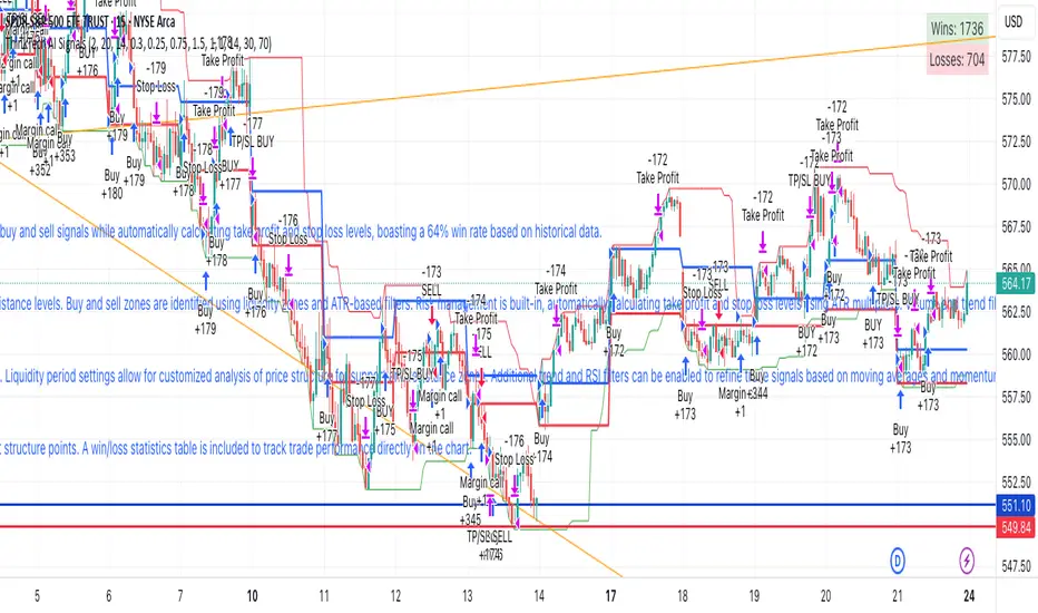
Mark Hours/Minutes (Formula + Minutes)This Pine Script code is a TradingView indicator that analyzes the hour and minutes of each candle in a 1-minute timeframe and plots a red triangle above the candle if one of the following conditions is met:
Sum/Difference Condition: The sum or the absolute difference of the hours and minutes is equal to 29, 35, or 71, with a tolerance of +/- 1.
Minutes Condition: The minutes are equal to 00, 29, or 35.
This indicator is based on the Goldbach theory and the "algo path" concept popularized by Hopiplaka, which posits that algorithmic trading paths often initiate from minute values of 00, 29, and 35. Use this indicator according to your trading strategy.
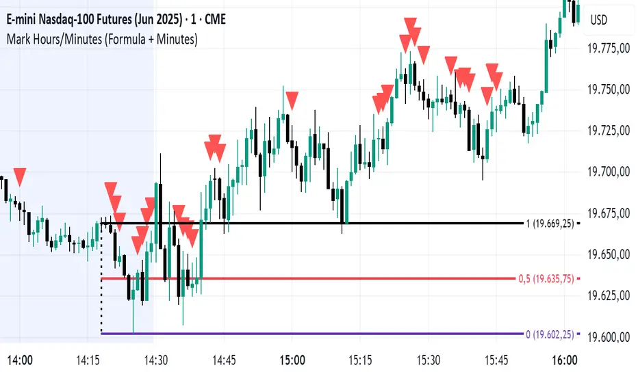
Stop/Take BoundsThe Stop/Take Bounds indicator is tool for setting dynamic stop-loss and take-profit levels based on percentage distance from the price. Unlike traditional ATR-based methods, this indicator allows traders to set stop levels as a fixed percentage of the price and define the take-profit multiple.
- Stop-loss distanceis determined as a percentage of the current price (e.g., 1% means the stop-loss is always 1% away from the price).
- Take-profit distance is calculated by multiplying the stop-loss distance by a user-defined multiplier (e.g., a multiplier of 2 places the take-profit level twice as far as the stop-loss).
- The indicator plots red lines for stop-loss levels and green lines for take-profit levels, making it easy to visualize risk-to-reward scenarios.
How to Use
1. Set Stop-Loss Distance (%) – Define how far the stop-loss should be from the price.
2. Set Take-Profit Multiplier – Choose how many times larger the take-profit should be compared to the stop-loss.
3. Apply to Long and Short Trades – The indicator automatically plots levels for both long and short positions.
4. Use in Manual or Algorithmic Trading – Ideal for discretionary traders as well as for integration into algorithmic strategies.
Use Cases
- Risk Management – Helps maintain disciplined risk-to-reward ratios.
- Strategy Development – Can be used in the creation of algorithmic trading systems.
- Trailing Stop Simulation – Can act as a trailing stop mechanism when used dynamically.
This indicator is a great addition to any trading strategy!
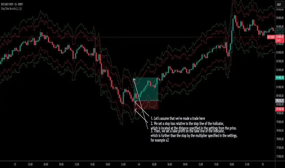
Quarterly Theory ICT 01 [TradingFinder] XAMD + Q1-Q4 Sessions🔵 Introduction
The Quarterly Theory ICT indicator is an advanced analytical system based on the concepts of ICT (Inner Circle Trader) and fractal time. It divides time into quarterly periods and accurately determines entry and exit points for trades by using the True Open as the starting point of each cycle. This system is applicable across various time frames including annual, monthly, weekly, daily, and even 90-minute sessions.
Time is divided into four quarters: in the first quarter (Q1), which is dedicated to the Accumulation phase, the market is in a consolidation state, laying the groundwork for a new trend; in the second quarter (Q2), allocated to the Manipulation phase (also known as Judas Swing), sudden price changes and false moves occur, marking the true starting point of a trend change; the third quarter (Q3) is dedicated to the Distribution phase, during which prices are broadly distributed and price volatility peaks; and the fourth quarter (Q4), corresponding to the Continuation/Reversal phase, either continues or reverses the previous trend.
By leveraging smart algorithms and technical analysis, this system identifies optimal price patterns and trading positions through the precise detection of stop-run and liquidity zones.
With the division of time into Q1 through Q4 and by incorporating key terms such as Quarterly Theory ICT, True Open, Accumulation, Manipulation (Judas Swing), Distribution, Continuation/Reversal, ICT, fractal time, smart algorithms, technical analysis, price patterns, trading positions, stop-run, and liquidity, this system enables traders to identify market trends and make informed trading decisions using real data and precise analysis.
♦ Important Note :
This indicator and the "Quarterly Theory ICT" concept have been developed based on material published in primary sources, notably the articles on Daye( traderdaye ) and Joshuuu . All copyright rights are reserved.
🔵 How to Use
The Quarterly Theory ICT strategy is built on dividing time into four distinct periods across various time frames such as annual, monthly, weekly, daily, and even 90-minute sessions. In this approach, time is segmented into four quarters, during which the phases of Accumulation, Manipulation (Judas Swing), Distribution, and Continuation/Reversal appear in a systematic and recurring manner.
The first segment (Q1) functions as the Accumulation phase, where the market consolidates and lays the foundation for future movement; the second segment (Q2) represents the Manipulation phase, during which prices experience sudden initial changes, and with the aid of the True Open concept, the real starting point of the market’s movement is determined; in the third segment (Q3), the Distribution phase takes place, where prices are widely dispersed and price volatility reaches its peak; and finally, the fourth segment (Q4) is recognized as the Continuation/Reversal phase, in which the previous trend either continues or reverses.
This strategy, by harnessing the concepts of fractal time and smart algorithms, enables precise analysis of price patterns across multiple time frames and, through the identification of key points such as stop-run and liquidity zones, assists traders in optimizing their trading positions. Utilizing real market data and dividing time into Q1 through Q4 allows for a comprehensive and multi-level technical analysis in which optimal entry and exit points are identified by comparing prices to the True Open.
Thus, by focusing on keywords like Quarterly Theory ICT, True Open, Accumulation, Manipulation, Distribution, Continuation/Reversal, ICT, fractal time, smart algorithms, technical analysis, price patterns, trading positions, stop-run, and liquidity, the Quarterly Theory ICT strategy acts as a coherent framework for predicting market trends and developing trading strategies.
🔵b]Settings
Cycle Display Mode: Determines whether the cycle is displayed on the chart or on the indicator panel.
Show Cycle: Enables or disables the display of the ranges corresponding to each quarter within the micro cycles (e.g., Q1/1, Q1/2, Q1/3, Q1/4, etc.).
Show Cycle Label: Toggles the display of textual labels for identifying the micro cycle phases (for example, Q1/1 or Q2/2).
Table Display Mode: Enables or disables the ability to display cycle information in a tabular format.
Show Table: Determines whether the table—which summarizes the phases (Q1 to Q4)—is displayed.
Show More Info: Adds additional details to the table, such as the name of the phase (Accumulation, Manipulation, Distribution, or Continuation/Reversal) or further specifics about each cycle.
🔵 Conclusion
Quarterly Theory ICT provides a fractal and recurring approach to analyzing price behavior by dividing time into four quarters (Q1, Q2, Q3, and Q4) and defining the True Open at the beginning of the second phase.
The Accumulation, Manipulation (Judas Swing), Distribution, and Continuation/Reversal phases repeat in each cycle, allowing traders to identify price patterns with greater precision across annual, monthly, weekly, daily, and even micro-level time frames.
Focusing on the True Open as the primary reference point enables faster recognition of potential trend changes and facilitates optimal management of trading positions. In summary, this strategy, based on ICT principles and fractal time concepts, offers a powerful framework for predicting future market movements, identifying optimal entry and exit points, and managing risk in various trading conditions.

AO/AC Trading Zones Strategy [Skyrexio] Overview
AO/AC Trading Zones Strategy leverages the combination of Awesome Oscillator (AO), Acceleration/Deceleration Indicator (AC), Williams Fractals, Williams Alligator and Exponential Moving Average (EMA) to obtain the high probability long setups. Moreover, strategy uses multi trades system, adding funds to long position if it considered that current trend has likely became stronger. Combination of AO and AC is used for creating so-called trading zones to create the signals, while Alligator and Fractal are used in conjunction as an approximation of short-term trend to filter them. At the same time EMA (default EMA's period = 100) is used as high probability long-term trend filter to open long trades only if it considers current price action as an uptrend. More information in "Methodology" and "Justification of Methodology" paragraphs. The strategy opens only long trades.
Unique Features
No fixed stop-loss and take profit: Instead of fixed stop-loss level strategy utilizes technical condition obtained by Fractals and Alligator to identify when current uptrend is likely to be over. In some special cases strategy uses AO and AC combination to trail profit (more information in "Methodology" and "Justification of Methodology" paragraphs)
Configurable Trading Periods: Users can tailor the strategy to specific market windows, adapting to different market conditions.
Multilayer trades opening system: strategy uses only 10% of capital in every trade and open up to 5 trades at the same time if script consider current trend as strong one.
Short and long term trend trade filters: strategy uses EMA as high probability long-term trend filter and Alligator and Fractal combination as a short-term one.
Methodology
The strategy opens long trade when the following price met the conditions:
1. Price closed above EMA (by default, period = 100). Crossover is not obligatory.
2. Combination of Alligator and Williams Fractals shall consider current trend as an upward (all details in "Justification of Methodology" paragraph)
3. Both AC and AO shall print two consecutive increasing values. At the price candle close which corresponds to this condition algorithm opens the first long trade with 10% of capital.
4. If combination of Alligator and Williams Fractals shall consider current trend has been changed from up to downtrend, all long trades will be closed, no matter how many trades has been opened.
5. If AO and AC both continue printing the rising values strategy opens the long trade on each candle close with 10% of capital while number of opened trades reaches 5.
6. If AO and AC both has printed 5 rising values in a row algorithm close all trades if candle's low below the low of the 5-th candle with rising AO and AC values in a row.
Script also has additional visuals. If second long trade has been opened simultaneously the Alligator's teeth line is plotted with the green color. Also for every trade in a row from 2 to 5 the label "Buy More" is also plotted just below the teeth line. With every next simultaneously opened trade the green color of the space between teeth and price became less transparent.
Strategy settings
In the inputs window user can setup strategy setting:
EMA Length (by default = 100, period of EMA, used for long-term trend filtering EMA calculation).
User can choose the optimal parameters during backtesting on certain price chart.
Justification of Methodology
Let's explore the key concepts of this strategy and understand how they work together. We'll begin with the simplest: the EMA.
The Exponential Moving Average (EMA) is a type of moving average that assigns greater weight to recent price data, making it more responsive to current market changes compared to the Simple Moving Average (SMA). This tool is widely used in technical analysis to identify trends and generate buy or sell signals. The EMA is calculated as follows:
1.Calculate the Smoothing Multiplier:
Multiplier = 2 / (n + 1), Where n is the number of periods.
2. EMA Calculation
EMA = (Current Price) × Multiplier + (Previous EMA) × (1 − Multiplier)
In this strategy, the EMA acts as a long-term trend filter. For instance, long trades are considered only when the price closes above the EMA (default: 100-period). This increases the likelihood of entering trades aligned with the prevailing trend.
Next, let’s discuss the short-term trend filter, which combines the Williams Alligator and Williams Fractals. Williams Alligator
Developed by Bill Williams, the Alligator is a technical indicator that identifies trends and potential market reversals. It consists of three smoothed moving averages:
Jaw (Blue Line): The slowest of the three, based on a 13-period smoothed moving average shifted 8 bars ahead.
Teeth (Red Line): The medium-speed line, derived from an 8-period smoothed moving average shifted 5 bars forward.
Lips (Green Line): The fastest line, calculated using a 5-period smoothed moving average shifted 3 bars forward.
When the lines diverge and align in order, the "Alligator" is "awake," signaling a strong trend. When the lines overlap or intertwine, the "Alligator" is "asleep," indicating a range-bound or sideways market. This indicator helps traders determine when to enter or avoid trades.
Fractals, another tool by Bill Williams, help identify potential reversal points on a price chart. A fractal forms over at least five consecutive bars, with the middle bar showing either:
Up Fractal: Occurs when the middle bar has a higher high than the two preceding and two following bars, suggesting a potential downward reversal.
Down Fractal: Happens when the middle bar shows a lower low than the surrounding two bars, hinting at a possible upward reversal.
Traders often use fractals alongside other indicators to confirm trends or reversals, enhancing decision-making accuracy.
How do these tools work together in this strategy? Let’s consider an example of an uptrend.
When the price breaks above an up fractal, it signals a potential bullish trend. This occurs because the up fractal represents a shift in market behavior, where a temporary high was formed due to selling pressure. If the price revisits this level and breaks through, it suggests the market sentiment has turned bullish.
The breakout must occur above the Alligator’s teeth line to confirm the trend. A breakout below the teeth is considered invalid, and the downtrend might still persist. Conversely, in a downtrend, the same logic applies with down fractals.
In this strategy if the most recent up fractal breakout occurs above the Alligator's teeth and follows the last down fractal breakout below the teeth, the algorithm identifies an uptrend. Long trades can be opened during this phase if a signal aligns. If the price breaks a down fractal below the teeth line during an uptrend, the strategy assumes the uptrend has ended and closes all open long trades.
By combining the EMA as a long-term trend filter with the Alligator and fractals as short-term filters, this approach increases the likelihood of opening profitable trades while staying aligned with market dynamics.
Now let's talk about the trading zones concept and its signals. To understand this we need to briefly introduce what is AO and AC. The Awesome Oscillator (AO), developed by Bill Williams, is a momentum indicator designed to measure market momentum by contrasting recent price movements with a longer-term historical perspective. It helps traders detect potential trend reversals and assess the strength of ongoing trends.
The formula for AO is as follows:
AO = SMA5(Median Price) − SMA34(Median Price)
where:
Median Price = (High + Low) / 2
SMA5 = 5-period Simple Moving Average of the Median Price
SMA 34 = 34-period Simple Moving Average of the Median Price
The Acceleration/Deceleration (AC) Indicator, introduced by Bill Williams, measures the rate of change in market momentum. It highlights shifts in the driving force of price movements and helps traders spot early signs of trend changes. The AC Indicator is particularly useful for identifying whether the current momentum is accelerating or decelerating, which can indicate potential reversals or continuations. For AC calculation we shall use the AO calculated above is the following formula:
AC = AO − SMA5(AO) , where SMA5(AO)is the 5-period Simple Moving Average of the Awesome Oscillator
When the AC is above the zero line and rising, it suggests accelerating upward momentum.
When the AC is below the zero line and falling, it indicates accelerating downward momentum.
When the AC is below zero line and rising it suggests the decelerating the downtrend momentum. When AC is above the zero line and falling, it suggests the decelerating the uptrend momentum.
Now let's discuss the trading zones concept and how it can create the signal. Zones are created by the combination of AO and AC. We can divide three zone types:
Greed zone: when the AO and AC both are rising
Red zone: when the AO and AC both are decreasing
Gray zone: when one of AO or AC is rising, the other is falling
Gray zone is considered as uncertainty. AC and AO are moving in the opposite direction. Strategy skip such price action to decrease the chance to stuck in the losing trade during potential sideways. Red zone is also not interesting for the algorithm because both indicators consider the trend as bearish, but strategy opens only long trades. It is waiting for the green zone to increase the chance to open trade in the direction of the potential uptrend. When we have 2 candles in a row in the green zone script executes a long trade with 10% of capital.
Two green zone candles in a row is considered by algorithm as a bullish trend, but now so strong, that's the reason why trade is going to be closed when the combination of Alligator and Fractals will consider the the trend change from bullish to bearish. If id did not happens, algorithm starts to count the green zone candles in a row. When we have 5 in a row script change the trade closing condition. Such situation is considered is a high probability strong bull market and all trades will be closed if candle's low will be lower than fifth green zone candle's low. This is used to increase probability to secure the profit. If long trades are initiated, the strategy continues utilizing subsequent signals until the total number of trades reaches a maximum of 5. Each trade uses 10% of capital.
Why we use trading zones signals? If currently strategy algorithm considers the high probability of the short-term uptrend with the Alligator and Fractals combination pointed out above and the long-term trend is also suggested by the EMA filter as bullish. Rising AC and AO values in the direction of the most likely main trend signaling that we have the high probability of the fastest bullish phase on the market. The main idea is to take part in such rapid moves and add trades if this move continues its acceleration according to indicators.
Backtest Results
Operating window: Date range of backtests is 2023.01.01 - 2024.12.31. It is chosen to let the strategy to close all opened positions.
Commission and Slippage: Includes a standard Binance commission of 0.1% and accounts for possible slippage over 5 ticks.
Initial capital: 10000 USDT
Percent of capital used in every trade: 10%
Maximum Single Position Loss: -9.49%
Maximum Single Profit: +24.33%
Net Profit: +4374.70 USDT (+43.75%)
Total Trades: 278 (39.57% win rate)
Profit Factor: 2.203
Maximum Accumulated Loss: 668.16 USDT (-5.43%)
Average Profit per Trade: 15.74 USDT (+1.37%)
Average Trade Duration: 60 hours
How to Use
Add the script to favorites for easy access.
Apply to the desired timeframe and chart (optimal performance observed on 4h BTC/USDT).
Configure settings using the dropdown choice list in the built-in menu.
Set up alerts to automate strategy positions through web hook with the text: {{strategy.order.alert_message}}
Disclaimer:
Educational and informational tool reflecting Skyrex commitment to informed trading. Past performance does not guarantee future results. Test strategies in a simulated environment before live implementation
These results are obtained with realistic parameters representing trading conditions observed at major exchanges such as Binance and with realistic trading portfolio usage parameters.
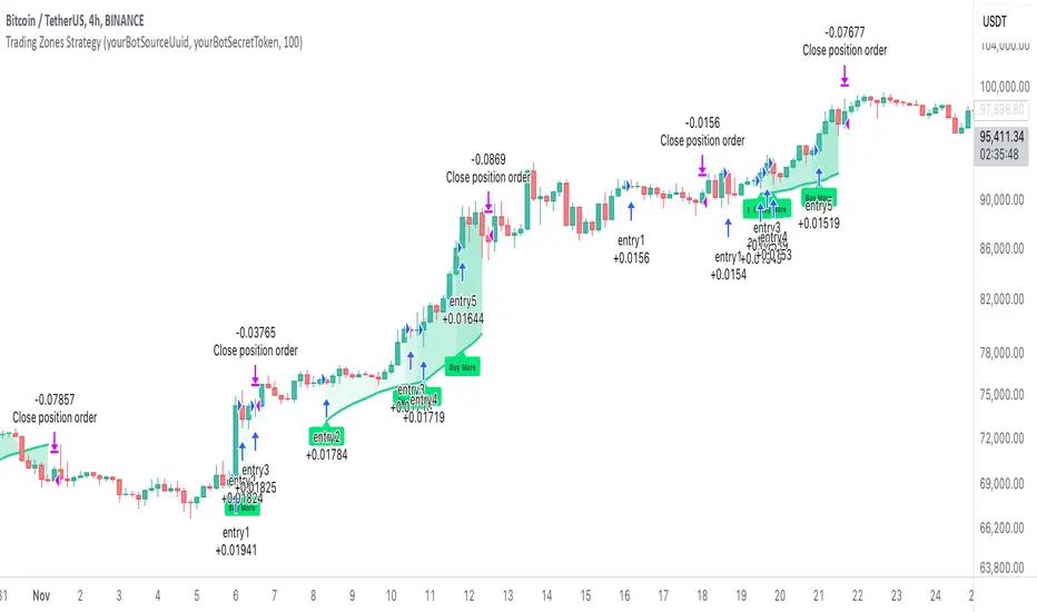
Arpeet MACDOverview
This strategy is based on the zero-lag version of the MACD (Moving Average Convergence Divergence) indicator, which captures short-term trends by quickly responding to price changes, enabling high-frequency trading. The strategy uses two moving averages with different periods (fast and slow lines) to construct the MACD indicator and introduces a zero-lag algorithm to eliminate the delay between the indicator and the price, improving the timeliness of signals. Additionally, the crossover of the signal line and the MACD line is used as buy and sell signals, and alerts are set up to help traders seize trading opportunities in a timely manner.
Strategy Principle
Calculate the EMA (Exponential Moving Average) or SMA (Simple Moving Average) of the fast line (default 12 periods) and slow line (default 26 periods).
Use the zero-lag algorithm to double-smooth the fast and slow lines, eliminating the delay between the indicator and the price.
The MACD line is formed by the difference between the zero-lag fast line and the zero-lag slow line.
The signal line is formed by the EMA (default 9 periods) or SMA of the MACD line.
The MACD histogram is formed by the difference between the MACD line and the signal line, with blue representing positive values and red representing negative values.
When the MACD line crosses the signal line from below and the crossover point is below the zero axis, a buy signal (blue dot) is generated.
When the MACD line crosses the signal line from above and the crossover point is above the zero axis, a sell signal (red dot) is generated.
The strategy automatically places orders based on the buy and sell signals and triggers corresponding alerts.
Advantage Analysis
The zero-lag algorithm effectively eliminates the delay between the indicator and the price, improving the timeliness and accuracy of signals.
The design of dual moving averages can better capture market trends and adapt to different market environments.
The MACD histogram intuitively reflects the comparison of bullish and bearish forces, assisting in trading decisions.
The automatic order placement and alert functions make it convenient for traders to seize trading opportunities in a timely manner, improving trading efficiency.
Risk Analysis
In volatile markets, frequent crossover signals may lead to overtrading and losses.
Improper parameter settings may cause signal distortion and affect strategy performance.
The strategy relies on historical data for calculations and has poor adaptability to sudden events and black swan events.
Optimization Direction
Introduce trend confirmation indicators, such as ADX, to filter out false signals in volatile markets.
Optimize parameters to find the best combination of fast and slow line periods and signal line periods, improving strategy stability.
Combine other technical indicators or fundamental factors to construct a multi-factor model, improving risk-adjusted returns of the strategy.
Introduce stop-loss and take-profit mechanisms to control single-trade risk.
Summary
The MACD Dual Crossover Zero Lag Trading Strategy achieves high-frequency trading by quickly responding to price changes and capturing short-term trends. The zero-lag algorithm and dual moving average design improve the timeliness and accuracy of signals. The strategy has certain advantages, such as intuitive signals and convenient operation, but also faces risks such as overtrading and parameter sensitivity. In the future, the strategy can be optimized by introducing trend confirmation indicators, parameter optimization, multi-factor models, etc., to improve the robustness and profitability of the strategy.
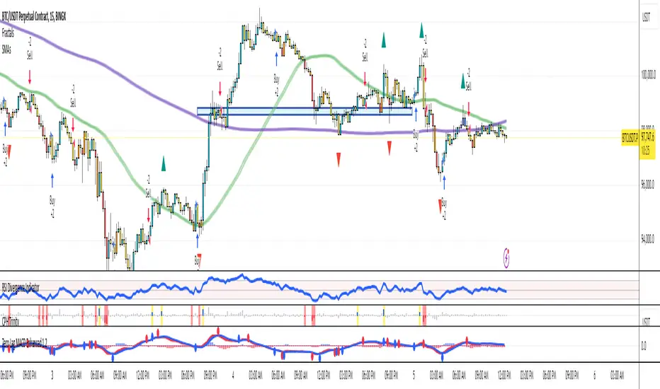
Classic Nacked Z-Score ArbitrageThe “Classic Naked Z-Score Arbitrage” strategy employs a statistical arbitrage model based on the Z-score of the price spread between two assets. This strategy follows the premise of pair trading, where two correlated assets, typically from the same market sector, are traded against each other to profit from relative price movements (Gatev, Goetzmann, & Rouwenhorst, 2006). The approach involves calculating the Z-score of the price spread between two assets to determine market inefficiencies and capitalize on short-term mispricing.
Methodology
Price Spread Calculation:
The strategy calculates the spread between the two selected assets (Asset A and Asset B), typically from different sectors or asset classes, on a daily timeframe.
Statistical Basis – Z-Score:
The Z-score is used as a measure of how far the current price spread deviates from its historical mean, using the standard deviation for normalization.
Trading Logic:
• Long Position:
A long position is initiated when the Z-score exceeds the predefined threshold (e.g., 2.0), indicating that Asset A is undervalued relative to Asset B. This signals an arbitrage opportunity where the trader buys Asset B and sells Asset A.
• Short Position:
A short position is entered when the Z-score falls below the negative threshold, indicating that Asset A is overvalued relative to Asset B. The strategy involves selling Asset B and buying Asset A.
Theoretical Foundation
This strategy is rooted in mean reversion theory, which posits that asset prices tend to return to their long-term average after temporary deviations. This form of arbitrage is widely used in statistical arbitrage and pair trading techniques, where investors seek to exploit short-term price inefficiencies between two assets that historically maintain a stable price relationship (Avery & Sibley, 2020).
Further, the Z-score is an effective tool for identifying significant deviations from the mean, which can be seen as a signal for the potential reversion of the price spread (Braucher, 2015). By capturing these inefficiencies, traders aim to profit from convergence or divergence between correlated assets.
Practical Application
The strategy aligns with the Financial Algorithmic Trading and Market Liquidity analysis, emphasizing the importance of statistical models and efficient execution (Harris, 2024). By utilizing a simple yet effective risk-reward mechanism based on the Z-score, the strategy contributes to the growing body of research on market liquidity, asset correlation, and algorithmic trading.
The integration of transaction costs and slippage ensures that the strategy accounts for practical trading limitations, helping to refine execution in real market conditions. These factors are vital in modern quantitative finance, where liquidity and execution risk can erode profits (Harris, 2024).
References
• Gatev, E., Goetzmann, W. N., & Rouwenhorst, K. G. (2006). Pairs Trading: Performance of a Relative-Value Arbitrage Rule. The Review of Financial Studies, 19(3), 1317-1343.
• Avery, C., & Sibley, D. (2020). Statistical Arbitrage: The Evolution and Practices of Quantitative Trading. Journal of Quantitative Finance, 18(5), 501-523.
• Braucher, J. (2015). Understanding the Z-Score in Trading. Journal of Financial Markets, 12(4), 225-239.
• Harris, L. (2024). Financial Algorithmic Trading and Market Liquidity: A Comprehensive Analysis. Journal of Financial Engineering, 7(1), 18-34.
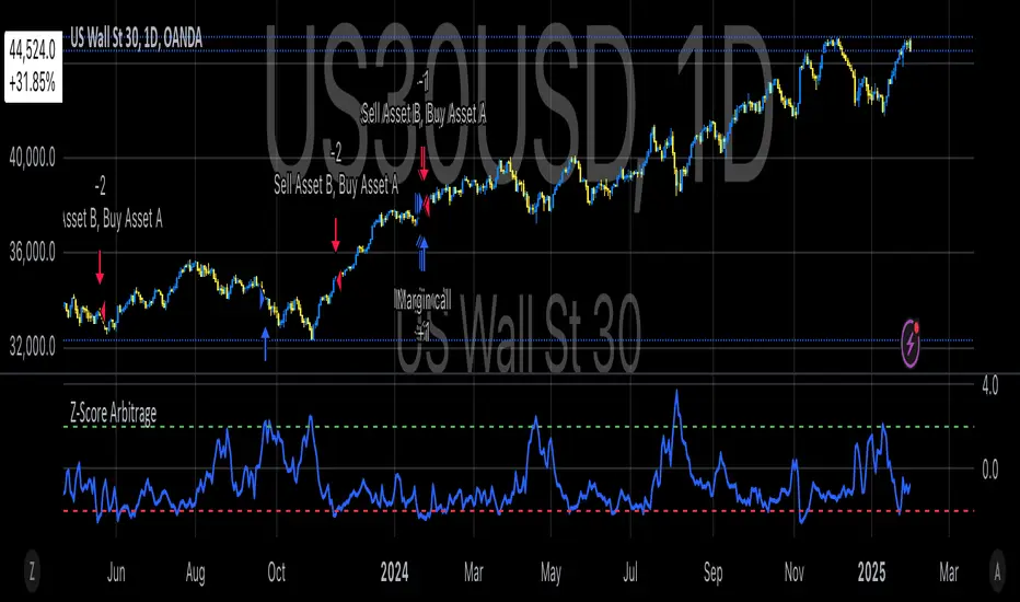
Auto-Adjusting Kalman Filter by TenozenNew year, new indicator! Auto-Adjusting Kalman Filter is an indicator designed to provide an adaptive approach to trend analysis. Using the Kalman Filter (a recursive algorithm used in signal processing), this algo dynamically adjusts to market conditions, offering traders a reliable way to identify trends and manage risk! In other words, it's a remaster of my previous indicator, Kalman Filter by Tenozen.
What's the difference with the previous indicator (Kalman Filter by Tenozen)?
The indicator adjusts its parameters (Q and R) in real-time using the Average True Range (ATR) as a measure of market volatility. This ensures the filter remains responsive during high-volatility periods and smooth during low-volatility conditions, optimizing its performance across different market environments.
The filter resets on a user-defined timeframe, aligning its calculations with dominant trends and reducing sensitivity to short-term noise. This helps maintain consistency with the broader market structure.
A confidence metric, derived from the deviation of price from the Kalman filter line (measured in ATR multiples), is visualized as a heatmap:
Green : Bullish confidence (higher values indicate stronger trends).
Red : Bearish confidence (higher values indicate stronger trends).
Gray : Neutral zone (low confidence, suggesting caution).
This provides a clear, objective measure of trend strength.
How it works?
The Kalman Filter estimates the "true" price by filtering out market noise. It operates in two steps, that is, prediction and update. Prediction is about projection the current state (price) forward. Update is about adjusting the prediction based on the latest price data. The filter's parameters (Q and R) are scaled using normalized ATR, ensuring adaptibility to changing market conditions. So it means that, Q (Process Noise) increases during high volatility, making the filter more responsive to price changes and R (Measurement Noise) increases during low volatility, smoothing out the filter to avoid overreacting to minor fluctuations. Also, the trend confidence is calculated based on the deviation of price from the Kalman filter line, measured in ATR multiples, this provides a quantifiable measure of trend strength, helping traders assess market conditions objectively.
How to use?
Use the Kalman Filter line to identify the prevailing trend direction. Trade in alignment with the filter's slope for higher-probability setups.
Look for pullbacks toward the Kalman Filter line during strong trends (high confidence zones)
Utilize the dynamic stop-loss and take-profit levels to manage risk and lock in profits
Confidence Heatmap provides an objective measure of market sentiment, helping traders avoid low-confidence (neutral) zones and focus on high-probability opportunities
Guess that's it! I hope this indicator helps! Let me know if you guys got some feedback! Ciao!