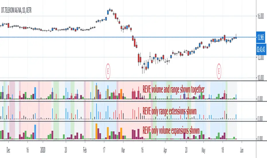
REVEREVE is abbreviation from Range Extension Volume Expansion. This indicator shows these against a background of momentum. The histogram and columns for the range and volume rises ara calculated with the same algorithm as I use in the Volume Range Events indicator, which I published before. Because this algorithm uses the same special function to assess 'normal' levels for volume and range and uses the same calculation for depicting the rises on a scale of zero through 100, it becomes possible to compare volume and range rises in the same chart panel and come to meaningful conclusions. Different from VolumeRangeEvents is that I don't attempt to show direction of the bars and columns by actually pointing up or down. However I did color the bars for range events according to direction if Close jumps more than 20 percent of ATR up or down either blue or red. If the wider range leads to nothing, i.e. a smaller jump than 20 percent, the color is black. You can teak this in the inputs. The volume colums ar colored according to two criteria, resulting in four colors (orange, blue, maroon, green). The first criterium is whether the expansion is climactic (orange, blue) or moderate (maroon, green). I assume that climactic (i.e. more than twice as much) volume marks the beginning or end of a trend. The second criterium looks at the range event that goes together with the volume event. If lots of volume lead to little change in range (blue, green), I assume that this volume originates from institutional traders who are accumulating or distributing. If wild price jumps occur with comparatively little volume (orange, maroon, or even no volume event) I assume that opportunistic are active, some times attributing to more volume.
For the background I use the same colors calculated with the same algorithm as in the Hull Agreement Indicator, which I published before. This way I try to predict trend changes by observation of REVE.
在腳本中搜尋"algo"
T3 ICL MACD STRATEGY
Backtested manually and received approx 60% winrate. Tradingview strategy tester is skewed because this program does not specify when to sell at profit target or at a stop loss.
Uses 1 min for entry and a longer time frame for confirmation (5,10,15, etc..) (Not sure what the yellow arrows are in the picture but they can be ignored)
Ideal Long Entry - The algo uses T3 moving average (T3) and the Ichimoku Conversion Line (ICL) to determine when to enter a long or short position. In this case we are going to showcase what causes the algo to alert long. It first checks to see if the the ICL is greater than T3. Once that condition is met T3 must be green in order to enter long and finally the last closing price has to be greater than the ICL. You can use the MACD to further verify a long trend as well!
Ideal Short Entry - The algo uses T3 moving average (T3) and the Ichimoku Conversion Line (ICL) to determine when to enter a long or short position. In this case we are going to showcase what causes the algo to alert short. It first checks to see if the the ICL is less than T3. Once that condition is met T3 must be red in order to enter short and finally the last closing price has to be less than the ICL. You can use the MACD to further verify a long trend as well!

[PX] Moon PhaseHello guys,
while scrolling through the public library, I was surprised that there was no Open-Source version of the Moon Phase indicator. All moon phase indicators in the public library were either protected or not exactly what I was looking for. There is a built-in "Moon Phase" indicator, but even for this one, we can't access its source code.
Therefore, I started searching for an algorithm that I could implement into PineScript.
So here we go, an Open-Source Moon Phase indicator. It comes with the option to color the background based on the recent moon. Compared to the built-in indicator, the moon is slightly shifted, because it is centered on the candle and not plotted between two candles like the built-in indicator is doing it.
Feel free to use the indicator for your analysis or build on top of it in an open-source fashion.
Happy trading,
paaax :)
Reference: This indicator is a converted and simplified version of the original javascript algorithm, which can be found here .

SMU Quantum Thermo BallsThis script is the enhanced version of Market Thermometer with one difference. This one has Quantum Thermo balls shooting out of the thermometer tube when overheated. Quantum psychology, Quantum observation, call it what you like
My scripts are designed to beat ALGO, so the behavior of indicators is not like traditional indicators. Don't try to overthink it and compare it to other established functions.
If you knew ALGo as much as I do, then you would also ditch old indicators and design your own weird scripts to match the ALGO's personality. Oh yes, each AlGo for each stock has its own programming personality. Most my scripts are tuned to beat SPX ALGO meniac
Enjoy and think outside the box, the only way to beat the ALGO

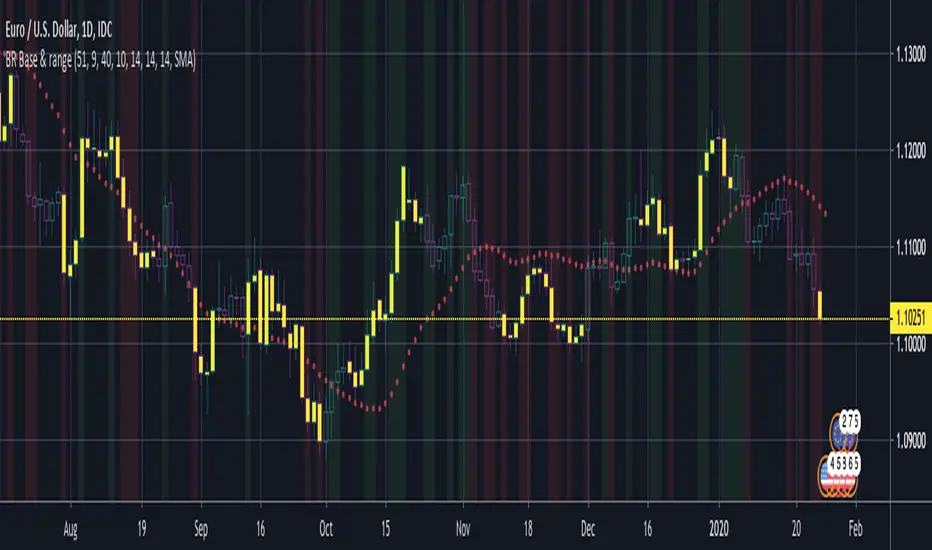
BERLIN Renegade - Baseline & RangeThis is the baseline and range candles part of a larger algorithm called the "BERLIN Renegade". It is based on the NNFX way of trading, with some modifications.
The baseline is used for price crossover signals, and consists of the LSMA. When price is below the baseline, the background turns red, and when it is above the baseline, the background turns green.
It also includes a modified version of the Range Identifier by LazyBear. This version calculates the same, but draws differently. It remove the baseline signal color if the Range Identifier signals there is a possible trading range forming.
The main way of identifying ranges is using the BERLIN Range Index. A panel version of this indicator is included in another part of the algorithm, but the bar color version is included here, to make the ranges even more visible and easier to avoid.
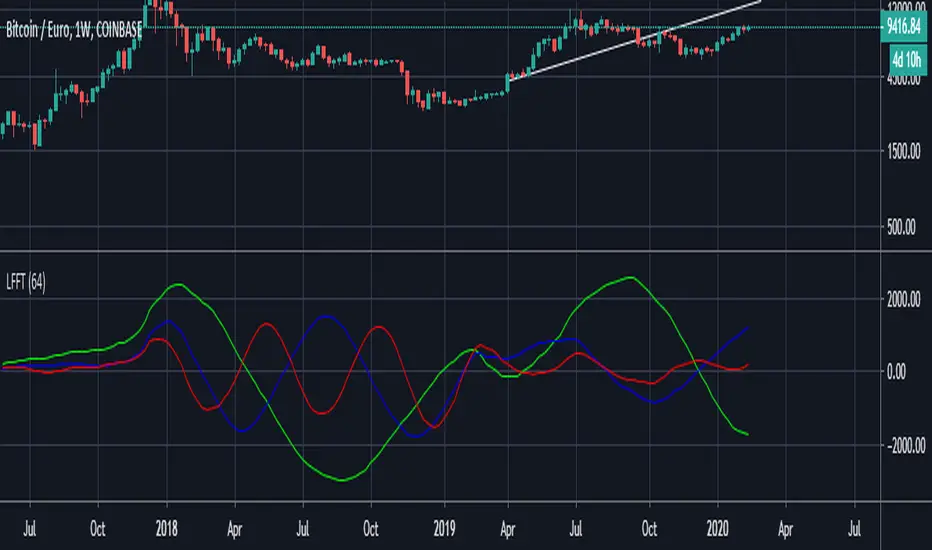
Low Frequency Fourier TransformThis Study uses the Real Discrete Fourier Transform algorithm to generate 3 sinusoids possibly indicative of future price.
I got information about this RDFT algorithm from "The Scientist and Engineer's Guide to Digital Signal Processing" By Steven W. Smith, Ph.D.
It has not been tested thoroughly yet, but it seems that that the RDFT isn't suited for predicting prices as the Frequency Domain Representation shows that the signal is similar to white noise, showing no significant peaks, indicative of very low periodicity of price movements.
Correlation MATRIX (Flexible version)Hey folks
A quick unrelated but interesting foreword
Hope you're all good and well and tanned
Me? I'm preparing the opening of my website where we're going to offer the Algorithm Builder Single Trend, Multiple Trends, Multi-Timeframe and plenty of others across many platforms (TradingView, FXCM, MT4, PRT). While others are at the beach and tanning (Yes I'm jealous, so what !?!), we're working our a** off to deliver an amazing looking website and great indicators and strategies for you guys.
Today I worked in including the Trade Manager Pro version and the Risk/Reward Pro version into all our Algorithm Builders. Here's a teaser
We're going to have a few indicators/strategies packages and subscriptions will open very soon.
The website should open in a few weeks and we still have loads to do ... (#no #summer #holidays #for #dave)
I see every message asking me to allow access to my Algorithm Builders but with the website opening shortly, it will be better for me to manage the trials from there - otherwise, it's duplicated and I can't follow all those requests
As you can probably all understand, it becomes very challenging to publish once a day with all that workload so I'll probably slow down (just a bit) and maybe posting once every 2/3 days until the website will be over (please forgive me for failing you). But once it will open, the daily publishing will resume again :) (here's when you're supposed to be clapping guys....)
While I'm so honored by all the likes, private messages and comments encouraging me, you have to realize that a script always takes me about 2/3 hours of work (with research, coding, debugging) but I'm doing it because I like it. Only pushing the brake a bit because of other constraints
INDICATOR OF THE DAY
I made a more flexible version of my Correlation Matrix .
You can now select the symbols you want and the matrix will update automatically !!! Let me repeat it once more because this is very cool... You can now select the symbols you want and the matrix will update automatically :)
Actually, I have nothing more to say about it... that's all :) Ah yes, I added a condition to detect negative correlation and they're being flagged with a black dot
Definition : Negative correlation or inverse correlation is a relationship between two variables whereby they move in opposite directions.
A negative correlation is a key concept in portfolio construction, as it enables the creation of diversified portfolios that can better withstand portfolio volatility and smooth out returns.
Correlation between two variables can vary widely over time. Stocks and bonds generally have a negative correlation, but in the decade to 2018, their correlation has ranged from -0.8 to 0.2. (Source : www.investopedia.com
See you maybe tomorrow or in a few days for another script/idea.
Be sure to hit the thumbs up to cheer me up as your likes will be the only sunlight I'll get for the next weeks.... because working on building a great offer for you guys.
Dave
____________________________________________________________
- I'm an officially approved PineEditor/LUA/MT4 approved mentor on codementor. You can request a coaching with me if you want and I'll teach you how to build kick-ass indicators and strategies
Jump on a 1 to 1 coaching with me
- You can also hire for a custom dev of your indicator/strategy/bot/chrome extension/python

SMA/pivot/Bollinger/MACD/RSI en pantalla gráficoMulti-indicador con los indicadores que empleo más pero sin añadir ventanas abajo.
Contiene:
Cruce de 3 medias móviles
La idea es no tenerlas en pantalla, pero están dibujadas también. Yo las dejo ocultas salvo que las quiera mirar para algo.
Lo que presento en pantalla es la media lenta con verde si el cruce de las 3 marca alcista, amarillo si no está claro y rojo si marca bajista.
Pivot
Normalmente los tengo ocultos pero los muestro cuando me interesa. Están todos aunque aparezcan 2 seguidos.
Bandas de Bollinger
No dibujo la línea central porque empleo la media como tal.
Parabollic SAR
Lo empleo para dibujar las ondas de Elliott como postula Matías Menéndez Larre en el capítulo 11 de su libro "Las ondas de Elliott". Así que, aunque se puede mostrar, lo mantengo oculto y lo que muestro es dónde cambia (SAR cambio).
MACD
No está dibujado porque necesitaría sacarlo del gráfico.
Marco en la parte superior cuándo la señal sobrepasa al MACD hacia arriba o hacia abajo con un flecha indicando el sentido de esta señal.
RSI
Similar al MACD pero en la parte inferior.
Probablemente, programe otro indicador para visualizar en una ventanita MACD, RSI y volumen todo junto. El volumen en la principal hay veces que no te permite ver bien alguna sombra y los otros 2 te quitan mucho espacio para graficar si los tienes permanentemente en 2 ventanas separadas.
DFT - Dominant Cycle Period 8-50 bars - John EhlerThis is the translation of discret cosine tranform (DCT) usage by John Ehler for finding dominant cycle period (DC).
The price is first filtered to remove aliasing noise(bellow 8 bars) and trend informations(above 50 bars), then the power is computed.
The trick here is to use a normalisation against the maximum power in order to get a good frequency resolution.
Current limitation in tradingview does not allow to display all of the periods, still the DC period is plot after beeing computed based on the center of gravity algo.
The DC period can be used to tune all of the indicators based on the cycles of the markets. For instance one can use this (DC period)/2 as an input for RSI.
Hope you find this of some interrest.
[naoligo] Simple ADXI'm publishing this indicator just for study purposes, because the result is exactly the same as DMI without the smoothing factor. It is exactly the same as ADX Wilder from MT5.
I was looking for the algorithm all over and it was a pain to find the right formula, meaning: one that would match with the built-in ones. After several study and comparison, I still didn't find the algorithm that match with the MT5's built-in simple ADX ...
Enjoy!

Patrones de entrada/salida V.1.0 -BETA-Este algoritmo intenta identificar patrones o fractales dentro de los movimientos de precios para dar señales de compra o venta de activos.

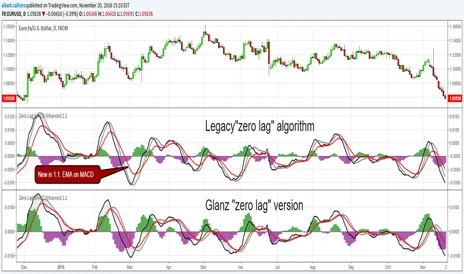
Zero Lag MACD Enhanced - Version 1.1ENHANCED ZERO LAG MACD
Version 1.1
Based on ZeroLag EMA - see Technical Analysis of Stocks and Commodities, April 2000
Original version by user Glaz. Thanks !
Ideas and code from @yassotreyo version.
Tweaked by Albert Callisto (AC)
New features:
Added original signal line formula
Added optional EMA on MACD
Added filling between the MACD and signal line
I looked at other versions of the zero lag and noticed that the histogram was slightly different. After looking at other zero lags on TV, I noticed that the algorithm implementation of Glanz generated a modified signal line. I decided to add the old version to be compliant with the original algorithm that you will find in other platforms like MT4, FXCM, etc.
So now you can choose if you want the original algorithm or Glanz version. It's up to you then to choose which one you prefer. I also added an extra EMA applied on the MACD. This is used in a system I am currently studying and can be of some interest to filter out false signals.
Acc/Dist. Cloud with Fractal Deviation Bands by @XeL_ArjonaACCUMULATION / DISTRIBUTION CLOUD with MORPHIC DEVIATION BANDS
Ver. 2.0.beta.23:08:2015
by Ricardo M. Arjona @XeL_Arjona
DISCLAIMER
The Following indicator/code IS NOT intended to be a formal investment advice or recommendation by the author, nor should be construed as such. Users will be fully responsible by their use regarding their own trading vehicles/assets.
The embedded code and ideas within this work are FREELY AND PUBLICLY available on the Web for NON LUCRATIVE ACTIVITIES and must remain as is.
Pine Script code MOD's and adaptations by @XeL_Arjona with special mention in regard of:
Buy (Bull) and Sell (Bear) "Power Balance Algorithm by Vadim Gimelfarb published at Stocks & Commodities V. 21:10 (68-72).
Custom Weighting Coefficient for Exponential Moving Average (nEMA) adaptation work by @XeL_Arjona with contribution help from @RicardoSantos at TradingView @pinescript chat room.
Morphic Numbers (PHI & Plastic) Pine Script adaptation from it's algebraic generation formulas by @XeL_Arjona
Fractal Deviation Bands idea by @XeL_Arjona
CHANGE LOG:
ACCUMULATION / DISTRIBUTION CLOUD: I decided to change it's name from the Buy to Sell Pressure. The code is essentially the same as older versions and they are the center core (VORTEX?) of all derived New stuff which are:
MORPHIC NUMBERS: The "Golden Ratio" expressed by the result of the constant "PHI" and the newer and same in characteristics "Plastic Number" expressed as "PN". For more information about this regard take a look at: HERE!
CUSTOM(K) EXPONENTIAL MOVING AVERAGE: Some code has cleaned from last version to include as custom function the nEMA , which use an additional input (K) to customise the way the "exponentially" is weighted from the custom array. For the purpose of this indicator, I implement a volatility algorithm using the Average True Range of last 9 periods multiplied by the morphic number used in the fractal study. (Golden Ratio as default) The result is very similar in response to classic EMA but tend to accelerate or decelerate much more responsive with wider bars presented in trending average.
FRACTAL DEVIATION BANDS: The main idea is based on the so useful Standard Deviation process to create Bands in favor of a multiplier (As John Bollinger used in it's own bands) from a custom array, in which for this case is the "Volume Pressure Moving Average" as the main Vortex for the "Fractallitly", so then apply as many "Child bands" using the older one as the new calculation array using the same morphic constant as multiplier (Like Fibonacci but with other approach rather than %ratios). Results are AWSOME! Market tend to accelerate or decelerate their Trend in favor of a Fractal approach. This bands try to catch them, so please experiment and feedback me your own observations.
EXTERNAL TICKER FOR VOLUME DATA: I Added a way to input volume data for this kind of study from external tickers. This is just a quicky-hack given that currently TradingView is not adding Volume to their Indexes so; maybe this is temporary by now. It seems that this part of the code is conflicting with intraday timeframes, so You are advised.
This CODE is versioned as BETA FOR TESTING PROPOSES. By now TradingView Admins are changing lot's of things internally, so maybe this could conflict with correct rendering of this study with special tickers or timeframes. I will try to code by itself just the core parts of this study in order to use them at discretion in other areas. ALL NEW IDEAS OR MODIFICATIONS to these indicator(s) are Welcome in favor to deploy a better and more accurate readings. I will be very glad to be notified at Twitter or TradingView accounts at: @XeL_Arjona

Bubble Risk ModelThe question of whether markets can be objectively assessed for overextension has occupied financial researchers for decades. Charles Kindleberger, in his seminal work "Manias, Panics, and Crashes" (1978), documented that speculative bubbles follow remarkably consistent patterns across centuries and asset classes. Yet identifying these patterns in real time remains notoriously difficult. The Bubble Risk Model attempts to address this challenge not by predicting crashes, but by systematically measuring the statistical characteristics that historically precede fragile market conditions.
The theoretical foundation draws from two distinct research traditions. The first is the work on regime-switching models pioneered by James Hamilton (1989), who demonstrated that economic time series often exhibit discrete shifts between different behavioral states. The second is the literature on tail risk and market fragility, most notably articulated by Nassim Taleb in "The Black Swan" (2007), which emphasizes that extreme events carry disproportionate importance and that traditional risk measures systematically underestimate their probability.
Rather than attempting to build a probabilistic model requiring assumptions about underlying distributions, the Bubble Risk Model operates as a deterministic state-inference system. This distinction matters. Lawrence Rabiner's foundational tutorial on Hidden Markov Models (1989) established the mathematical framework for inferring hidden states from observable data through Bayesian updating. The present model borrows the conceptual architecture of states and transitions but replaces probabilistic inference with rule-based logic. States are not computed through forward-backward algorithms but inferred through deterministic thresholds. This trade-off sacrifices theoretical elegance for practical robustness and interpretability.
The measurement framework rests on four empirically grounded components. The first captures trailing twelve-month returns, reflecting the well-documented momentum effect identified by Jegadeesh and Titman (1993), who found that securities with strong past performance tend to continue outperforming over intermediate horizons. The second component measures trend persistence as the proportion of positive daily returns over a quarterly window, drawing on the research by Campbell and Shiller (1988) showing that price trends exhibit serial correlation that deviates from random walk assumptions. The third normalizes the distance between current prices and their long-term moving average by volatility, addressing the cross-sectional comparability problem noted by Fama and French (1992) when analyzing assets with different variance characteristics. The fourth component calculates return efficiency as the ratio of returns to realized volatility, a concept related to the Sharpe ratio but stripped of distributional assumptions that often fail in practice.
The aggregation methodology deliberately prioritizes worst-case scenarios. Rather than averaging component scores, the model uses quantile-based aggregation with an explicit tail penalty. This design choice reflects the asymmetric error costs in bubble detection: failing to identify fragility carries greater consequences than occasional false positives. The approach aligns with the precautionary principle advocated by Taleb and colleagues in their work on fragility and antifragility (2012), which argues that systems exposed to tail risks require conservative assessment frameworks.
Normalization presents a particular challenge. Raw metrics like year-over-year returns are not directly comparable across asset classes with different volatility profiles. The model addresses this through percentile ranking over multiple historical windows, typically two and five years. This dual-window approach provides regime stability, preventing the normalization from adapting too quickly during extended bull markets where elevated readings become statistically normal. The methodology draws on the concept of lookback bias documented by Lo and MacKinlay (1990), who demonstrated that single-window statistical measures can produce misleading results when market regimes shift.
The state machine introduces controlled inertia into the system. Once the model enters a particular state, transitions become progressively more difficult as the state matures. This transition resistance mechanism prevents rapid oscillation near threshold boundaries, a problem that plagues many indicator-based systems. The concept parallels the hysteresis effects described in economic literature by Dixit (1989), where systems exhibit path dependence and resist returning to previous states even when underlying conditions change.
Volatility regime detection adds contextual interpretation. Research by Engle (1982) on autoregressive conditional heteroskedasticity established that volatility clusters, with periods of high volatility tending to follow other high-volatility periods. The model scales its maturity thresholds inversely with volatility: in calm markets, states mature slowly and persist longer; in turbulent markets, information decays faster and states become more transient. This adaptive behavior reflects the empirical observation that low-volatility environments often precede significant market dislocations, as documented by Brunnermeier and Pedersen (2009) in their work on liquidity spirals.
The confidence metric addresses internal model consistency. When individual components diverge substantially, the overall score becomes less reliable regardless of its absolute level. This approach draws on ensemble methods in machine learning, where disagreement among predictors signals increased uncertainty. Dietterich (2000) provides theoretical justification for this principle, demonstrating that ensemble disagreement correlates with prediction error.
Distribution drift detection monitors whether the model's calibration remains valid. By comparing recent score distributions to longer historical baselines, the model can identify when market structure has shifted sufficiently to potentially invalidate its historical percentile rankings. This self-diagnostic capability reflects the concern raised by Andrews (1993) about parameter instability in time series models, where structural breaks can render previously estimated relationships unreliable.
The cross-asset analysis extends the framework beyond individual securities. By calculating scores for multiple asset classes simultaneously and measuring their correlation, the model distinguishes between idiosyncratic overextension affecting a single asset and systemic conditions affecting markets broadly. This differentiation matters for portfolio construction, as documented by Longin and Solnik (2001), who found that correlations between international equity markets increase significantly during periods of market stress.
Several limitations deserve explicit acknowledgment. The model cannot identify timing. Overextended conditions can persist far longer than rational analysis might suggest, a phenomenon documented by Shiller (2000) in his analysis of speculative episodes. The model provides no mechanism for determining when fragile conditions will resolve. Additionally, the cross-asset analysis lacks lead-lag detection, meaning it cannot distinguish whether assets became overextended simultaneously or sequentially. Finally, the rule-based nature of state inference means the model cannot express graduated probability assessments; states are discrete rather than continuous.
The philosophical stance underlying the model is one of epistemic humility. It does not claim to identify bubbles definitively or predict their collapse. Instead, it provides a systematic framework for measuring characteristics that have historically been associated with fragile market conditions. The distinction between information and action remains the user's responsibility. States describe current conditions; how to respond to those conditions requires judgment that no quantitative model can provide.
Practical guide for traders
This section translates the model's outputs into actionable intelligence for both retail traders managing personal portfolios and professional traders operating within institutional frameworks. The interpretation differs not in kind but in scale and consequence.
Understanding the score
The primary output is a continuous score ranging from zero to one. Lower scores indicate elevated bubble risk; higher scores suggest more sustainable market conditions. This inverse relationship may seem counterintuitive but reflects the model's construction: it measures how extreme current conditions are relative to historical norms, with extremity mapping to fragility.
A score above 0.50 generally indicates normal market conditions where standard investment approaches remain appropriate. Scores between 0.30 and 0.50 represent an elevated zone where caution is warranted but not alarm. Scores below 0.30 enter the extreme territory where historical precedent suggests increased fragility. These thresholds are not magical boundaries but represent statistical rarity: a score below 0.30 indicates conditions that occur in roughly the bottom quintile of historical observations.
For retail traders, a score in the normal range means continuing with established strategies without modification. In the elevated range, this might mean pausing new position additions while maintaining existing holdings. In the extreme range, retail traders should consider whether their portfolio could withstand a significant drawdown and whether their time horizon permits waiting for recovery. For professional traders, the score integrates into broader risk frameworks: normal conditions permit full risk budgets, elevated conditions might trigger reduced position sizing or tighter stop losses, and extreme conditions could warrant defensive positioning or increased hedging activity.
Reading the states
The model classifies conditions into three discrete states: Normal, Elevated, and Extreme. These states differ from the continuous score by incorporating persistence and transition resistance. A market can have a score temporarily dipping below 0.30 without triggering an Extreme state if the condition proves transient.
The Normal state indicates business as usual. Market conditions fall within historical norms across all measured dimensions. For retail traders, this means standard portfolio management applies. For professional traders, full strategy deployment remains appropriate with normal risk parameters.
The Elevated state signals heightened attention. At least one dimension of market behavior has moved outside normal ranges, though not to extreme levels. Retail traders should review portfolio concentration and ensure diversification remains intact. Professional traders might reduce leverage slightly, tighten risk limits, or increase monitoring frequency.
The Extreme state represents statistically rare conditions. Multiple dimensions show readings that historically occur infrequently. Retail traders should seriously evaluate whether they can tolerate potential drawdowns and consider reducing exposure to volatile assets. Professional traders should implement defensive protocols, potentially reducing gross exposure, increasing cash allocations, or adding protective positions.
Interpreting transitions
State transitions carry more information than states themselves. The model tracks whether conditions are entering, persisting in, or exiting particular states.
An Entry into Extreme represents the most important signal. It indicates a regime shift from normal or elevated conditions into territory associated with historical fragility. For retail traders, this warrants immediate portfolio review. For professional traders, this typically triggers predefined defensive protocols.
Persistence in a state indicates stability. Whether Normal or Extreme, persistence suggests the current regime has become established. For retail traders, persistence in Extreme over extended periods actually reduces immediate concern; the dangerous moment was the entry, not the continuation. For professional traders, persistent Extreme states require maintained vigilance but do not necessarily demand additional action beyond what the initial entry triggered.
An Exit from Extreme suggests improving conditions. For retail traders, this might warrant cautious return to normal positioning over time. For professional traders, exits permit gradual normalization of risk budgets, though institutional memory typically counsels slower reentry than the mathematical signal might suggest.
Duration and its meaning
The model distinguishes between Tactical, Accelerating, and Structural durations in critical zones.
Tactical duration (10-39 bars in critical territory) represents short-term overextension. Many Tactical episodes resolve without significant market disruption. Retail traders should note the condition but need not take dramatic action. Professional traders might implement modest hedges or reduce marginal positions.
Accelerating indicates Tactical duration combined with actively deteriorating scores. This combination historically precedes more significant corrections. Retail traders should consider lightening positions in their most volatile holdings. Professional traders typically implement more substantial hedges.
Structural duration (40+ bars in critical territory) indicates persistent overextension that has become a market feature rather than a temporary condition. Paradoxically, Structural conditions are both more concerning and less immediately actionable than Accelerating conditions. The market has demonstrated ability to sustain extreme readings. Retail traders should maintain heightened awareness but recognize that timing remains impossible. Professional traders often find Structural conditions require strategy adaptation rather than simple defensive positioning.
Confidence and what it tells you
The Confidence reading indicates internal model consistency. High confidence means all four underlying components agree in their assessment. Low confidence means components diverge significantly.
High confidence combined with Extreme state represents the clearest signal. The model is both indicating fragility and agreeing with itself about that assessment. Retail and professional traders alike should treat this combination with maximum seriousness.
Low confidence in any state reduces signal reliability. For retail traders, low confidence suggests waiting for clearer conditions before making significant portfolio changes. For professional traders, low confidence warrants increased skepticism about the score and potentially reduced position sizing in either direction.
Alignment and model health
The Alignment indicator monitors whether the model's calibration remains valid relative to recent market behavior.
Good alignment means recent score distributions match longer-term historical patterns. The model's percentile rankings remain meaningful. Both retail and professional traders can interpret scores at face value.
Degraded alignment indicates that recent market behavior has shifted somewhat from historical norms. Scores remain interpretable but with reduced precision. Retail traders should apply wider uncertainty bands to their interpretation. Professional traders might reduce position sizing slightly or require additional confirmation before acting.
Poor alignment signals significant distribution shift. The model may be comparing current conditions to an increasingly irrelevant historical baseline. Retail traders should rely more heavily on other information sources during Poor alignment periods. Professional traders typically reduce model weight in their decision frameworks until alignment recovers.
Volatility regime context
The volatility regime provides essential context for score interpretation.
Low volatility combined with Extreme state creates maximum concern. Research consistently shows that low-volatility environments can precede significant market dislocations. The market's apparent calm masks underlying fragility. Retail traders should recognize that low volatility does not mean low risk; it often means compressed risk premiums that will eventually normalize, potentially violently. Professional traders typically maintain or increase defensive positioning despite the market's calm appearance.
High volatility combined with Extreme state is actually less immediately concerning than low volatility. The market has already acknowledged stress; risk premiums have expanded; potential sellers may have already sold. Retail traders should resist the urge to panic sell during high-volatility extremes, as much of the adjustment may have already occurred. Professional traders recognize that high-volatility extremes often represent better entry points than low-volatility extremes.
Normal volatility requires no regime adjustment to interpretation. Scores mean what they appear to mean.
Cross-asset analysis
When enabled, the model calculates scores for multiple asset classes simultaneously, enabling systemic versus idiosyncratic risk assessment.
Systemic risk (multiple assets in Extreme with high correlation) indicates market-wide fragility. Diversification benefits are reduced precisely when most needed. Retail traders should recognize that their portfolio's apparent diversification may not protect them during systemic events. Professional traders implement cross-asset hedges and consider tail-risk protection.
Broad risk (multiple assets in Extreme with low correlation) suggests widespread but potentially unrelated overextension. Diversification may still provide some protection. Retail traders can take modest comfort in genuine diversification. Professional traders analyze which assets might offer relative value.
Isolated risk (single asset in Extreme while others remain Normal) indicates asset-specific rather than market-wide conditions. Retail traders holding the affected asset should evaluate their position specifically. Professional traders may find relative value opportunities going long unaffected assets against the extended one.
Scattered risk represents a few assets showing elevation without clear pattern. This typically warrants monitoring rather than action for both retail and professional traders.
Parameter guidance
The Short Percentile parameter (default 504 bars, approximately two years) controls the shorter normalization window. Increasing this value makes the model more conservative, requiring more extreme readings to flag concern. Retail traders should generally leave this at default. Professional traders might increase it for assets with shorter reliable history.
The Long Percentile parameter (default 1260 bars, approximately five years) controls the longer normalization window. This provides regime stability. Again, default settings suit most applications.
The Critical Threshold (default 0.30) determines where the Extreme state boundary lies. Lowering this value makes the model less sensitive, flagging fewer Extreme conditions. Raising it increases sensitivity. Retail traders seeking fewer false alarms might lower this to 0.25. Professional traders seeking earlier warning might raise it to 0.35.
The Structural Duration parameter (default 40 bars) determines when Tactical conditions become Structural. Shorter values provide earlier Structural classification. Longer values require more persistence before reclassification.
The State Maturity and Transition Resistance parameters control how readily the model changes states. Higher values create more stable states with fewer transitions. Lower values create more responsive but potentially noisier state changes. Default settings balance responsiveness against stability.
The Adaptive Smoothing parameters control how the model filters noise. In extreme zones, longer smoothing periods reduce whipsaws but increase lag. In normal zones, shorter periods maintain responsiveness. Most traders should leave these at defaults.
What the model cannot do
The model cannot predict when overextended conditions will resolve. Markets can remain irrational longer than any trader can remain solvent, as the saying goes. Extended Extreme readings may persist for months or even years before any correction materializes.
The model cannot distinguish between healthy bull markets and dangerous bubbles in their early stages. Both initially appear as strong returns and positive momentum. The model begins flagging concern only when statistical extremity develops, which may occur well into an advance.
The model cannot account for fundamental changes in market structure. If a new paradigm genuinely justifies higher valuations (rare but not impossible), the model will continue flagging extremity against historical norms that may no longer apply. The Alignment indicator provides partial protection against this failure mode but cannot eliminate it.
The model cannot replace judgment. It provides systematic measurement of conditions that have historically preceded fragility. Whether and how to act on that measurement remains entirely the trader's responsibility. Retail traders must still evaluate their personal circumstances, time horizons, and risk tolerance. Professional traders must still integrate model output with fundamental analysis, portfolio constraints, and client mandates.
References
Andrews, D.W.K. (1993). Tests for Parameter Instability and Structural Change with Unknown Change Point. Econometrica, 61(4).
Brunnermeier, M.K., & Pedersen, L.H. (2009). Market Liquidity and Funding Liquidity. Review of Financial Studies, 22(6).
Campbell, J.Y., & Shiller, R.J. (1988). Stock Prices, Earnings, and Expected Dividends. Journal of Finance, 43(3).
Dietterich, T.G. (2000). Ensemble Methods in Machine Learning. Multiple Classifier Systems.
Dixit, A. (1989). Entry and Exit Decisions under Uncertainty. Journal of Political Economy, 97(3).
Engle, R.F. (1982). Autoregressive Conditional Heteroscedasticity with Estimates of the Variance of United Kingdom Inflation. Econometrica, 50(4).
Fama, E.F., & French, K.R. (1992). The Cross-Section of Expected Stock Returns. Journal of Finance, 47(2).
Hamilton, J.D. (1989). A New Approach to the Economic Analysis of Nonstationary Time Series and the Business Cycle. Econometrica, 57(2).
Jegadeesh, N., & Titman, S. (1993). Returns to Buying Winners and Selling Losers: Implications for Stock Market Efficiency. Journal of Finance, 48(1).
Kindleberger, C.P. (1978). Manias, Panics, and Crashes: A History of Financial Crises. Basic Books.
Lo, A.W., & MacKinlay, A.C. (1990). Data-Snooping Biases in Tests of Financial Asset Pricing Models. Review of Financial Studies, 3(3).
Longin, F., & Solnik, B. (2001). Extreme Correlation of International Equity Markets. Journal of Finance, 56(2).
Rabiner, L.R. (1989). A Tutorial on Hidden Markov Models and Selected Applications in Speech Recognition. Proceedings of the IEEE, 77(2).
Shiller, R.J. (2000). Irrational Exuberance. Princeton University Press.
Taleb, N.N. (2007). The Black Swan: The Impact of the Highly Improbable. Random House.
Taleb, N.N., & Douady, R. (2012). Mathematical Definition, Mapping, and Detection of (Anti)Fragility. Quantitative Finance, 13(11).

SA Range Rank ALOG PRESSURE 1 AND 2This is a 4-candle market mechanic:
Bull pattern (orange)
Impulse up (strong bullish candle)
Stall / absorption (small candle; indecision)
Trap down (small bearish candle that fails to continue down)
Ignition up (bull candle breaks above the micro-range)
Bear pattern (yellow)
Impulse down
Stall / absorption
Trap up
Ignition down (bear candle breaks below micro-range)
Interpretation:
This is “pressure → absorption → reversal ignition.”
It’s meant to catch the moment where retail commits late and gets forced out.
How to Trade It on 15-Minute
15m is your structure execution timeframe: fewer signals, higher quality.
Recommended Indicator Settings (15m /NQ)
For CLEAN version (best baseline)
Sensitivity: BALANCED
Require VWAP bias: ON
Require EMA slope: ON
Targets: ON
Line extend bars: 40–60
For PRO (Looser) (more signals)
Keep defaults, then:
useVWAP: ON
useTrend: ON
useRetestHold: OFF (turn ON only if you want A+ only)
15m Entry Rules (Simple + Effective)
BULL (orange)
Enter on:
The close of the signal candle or
Next candle if it holds above the breakout area (safer)
BEAR (yellow)
Enter on:
The close of the signal candle or
Next candle if it holds below the breakdown area (safer)
15m Risk & Targets
STOP = the STOP line
PT1 = first scale / partial
PT2 = runner target
Suggested execution
Take 50–70% off at PT1
Move stop to breakeven after PT1 (optional)
Hold remainder to PT2 or trail
When to IGNORE a 15m signal
Skip it if:
Signal prints into a major level (prior day high/low, VWAP bands, overnight high/low)
You’re in the middle of chop and ATR is collapsing hard
The signal prints right before major news (CPI/FOMC)
How to Trade It on 1-Minute
1m is your execution / microstructure timeframe: more signals, faster decisions.
Recommended Indicator Settings (1m /NQ)
CLEAN version (to avoid spam)
Sensitivity: STRICT or BALANCED
VWAP: ON
EMA slope: ON
Targets: ON
PRO (Looser) (if you WANT frequent scalps)
Defaults are fine, but do:
useRetestHold: ON (recommended for 1m to avoid fake-outs)
Keep VWAP ON
1m Entry Rules (must be disciplined)
Best entry method (highest probability)
Wait for signal
Enter on the first retest/hold (if using retest hold)
If not using retest hold: enter only if next bar does not immediately reverse
1m Risk & Targets
PTs are ATR-based. On 1m, ATR is smaller, so targets are naturally tighter.
Use PT1 as a fast scalp, PT2 as stretch.
Suggested execution
Take 70–80% off at PT1
Very small runner to PT2
When to ignore 1m signals
Skip if:
It’s printing against the 15m direction
Price is whipping above/below VWAP repeatedly (chop)
ATR is extremely low (fake signals)
5) “Permission Layer” (15m → 1m workflow)
This is the cleanest way to combine both:
Step 1 (15m)
Use 15m signals as permission:
If 15m prints BULL, then you ONLY take 1m BULL signals for the next 30–90 minutes
If 15m prints BEAR, then you ONLY take 1m BEAR signals
Step 2 (1m)
Use 1m signals for entries and re-entries, with tighter targets.
This matches your framework:
15m = “structure gives permission”
1m = “execution extracts”
6) Ready-to-paste TradingView Descriptions
A) Description for SA 4-Candle Cycle — CLEAN (ATR Auto Targets)
Paste this into your TradingView script description:
SA 4-Candle Cycle (CLEAN) identifies a repeatable market mechanic: impulse → stall/absorption → trap → ignition.
Orange BULL signals print when a 4-candle bullish reversal/continuation cycle completes and price confirms by breaking above the micro-range. Yellow BEAR signals print on the inverse breakdown cycle.
This tool includes ATR-adaptive targets:
STOP = volatility-scaled invalidation level (optionally uses the swing reference candle)
PT1 / PT2 = first and second profit objectives scaled by ATR
Best use
15m: primary signal timeframe (higher quality, fewer signals). Enable VWAP and EMA slope filters for best results.
1m: execution timeframe for scalps and re-entries. Use STRICT/BALANCED sensitivity to reduce noise.
Risk note: This is not financial advice. Always manage risk and confirm with your larger structure levels.
B) Description for SA 4-Candle ATR-Adaptive Cycle — PRO (Looser) + Auto Targets
Paste this into your TradingView script description:
SA 4-Candle Cycle (PRO/Looser) is a higher-frequency variant of the 4-candle cycle model designed to print more signals while still respecting ATR-based structure. It detects impulse → absorption → trap → ignition sequences and plots ATR-scaled STOP, PT1, and PT2 levels automatically.
Best use
15m: use VWAP + EMA slope filters ON for higher probability.
1m: enable retest/hold if you want A+ entries only and fewer false breaks.
This version is ideal when you want earlier detection and more opportunities, while still keeping the risk framework systematic through ATR-adaptive targets.
Risk note: This is not financial advice. Use strict risk management.
Quick Recommendations (so you don’t get flooded)
If you want very high probability:
15m: CLEAN + BALANCED + VWAP ON + EMA slope ON
1m: PRO + VWAP ON + RetestHold ON + (optionally EMA slope ON)

Cup & Handle (Zeiierman)█ Overview
Cup & Handle (Zeiierman) is a classic continuation-pattern scanner that detects both bullish Cup+Handle and bearish Inverted Cup+Handle structures using a compact pivot stream. It’s designed to highlight rounded reversals back to a “rim” level, followed by a smaller pullback (“handle”) before a potential continuation move.
⚪ What It Detects
A Cup & Handle (Bull) forms when price makes a rounded decline from a left rim, bottoms, then climbs back to a similar right rim. After returning to the rim, price forms a handle (a smaller pullback) that stays within an allowed retracement range. This pattern often precedes a bullish continuation attempt.
An Inverted Cup & Handle (Bear) is the mirrored version. Price makes a rounded rise to a left rim, tops, then declines back to a similar right rim. After returning to that rim, price forms a handle (a smaller bounce) that stays within the allowed retracement range. This pattern often precedes a bearish continuation attempt.
█ How It Works
⚪ 1) Pivot Extraction (Swing Compression)
The script first converts raw candles into a small set of meaningful swing pivots using ta.pivothigh() and ta.pivotlow() with Pivot span. A pivot is accepted only after it is confirmed by the lookback window, which helps reduce noise.
Key effect:
Higher Pivot span = fewer, stronger pivots (cleaner patterns)
Lower Pivot span = more pivots (more patterns, more noise)
⚪ 2) Pattern Framing (4-Point Structure)
When at least four pivots exist, the script maps them into a fixed sequence:
For a bull Cup+Handle sequence: High → Low → High → Low
These are treated as:
L = left rim pivot
B = cup bottom pivot
R = right rim pivot
H = handle pivot
For a bear inverted Cup+Handle sequence: Low → High → Low → High
Mapped similarly, but inverted.
This “4-pivot” structure is the minimum shape needed to define a cup and a handle without overfitting.
⚪ 3) Rim Similarity Filter (Cup Quality Control)
The script checks if the left rim and right rim are close enough to be considered a proper cup rim:
Rim similarity tolerance (%) controls this.
Lower tolerance = only very clean symmetric rims
Higher tolerance = allows uneven rims (more detections)
⚪ 4) Handle Depth Filter (Reject Weak or Messy Handles)
The handle is validated by measuring how deep it retraces relative to the cup depth:
Handle Retraction = |rim − handle| / |rim − bottom|
The handle must fall between:
Handle retrace min
Handle retrace max
This prevents:
tiny “non-handle” wiggles (too shallow)
deep pullbacks that break the structure (too deep)
█ How to Use
⚪ Interpreting a Bull Cup & Handle
Treat it like a continuation setup built around a key breakout level:
Cup forms
Handle forms
Breakout happens above this level
Once price returns to this breakout zone and the handle stays controlled, the structure may attempt to continue upward.
Common behaviors after a clean signal:
Push above the breakout level
Brief retest/acceptance near the breakout zone
Continuation toward the projected target if momentum holds
⚪ Interpreting a Bear Inverted Cup & Handle
Treat it like a bearish continuation/rollover setup built around the same breakout concept:
Cup forms (inverted)
Handle forms
Breakout happens below this level
Once price returns to this breakout zone and the handle stays controlled, the structure may attempt to continue downward.
Common behaviors after a clean signal:
Drop below the breakout level
Retest from underneath
Continuation toward the projected target if selling pressure persists
█ Settings
Pivot span – pivot sensitivity. Higher = smoother pivots, fewer signals. Lower = more pivots, more signals/noise.
Rim similarity tolerance (%) – rim quality filter. Lower = stricter symmetry, higher = more permissive detection.
Handle retrace min – minimum handle depth (filters weak handles).
Handle retrace max – maximum handle depth (filters messy/deep handles).
Invalidation (handle max retrace %) – “maximum tolerated damage” for handle move before the structure is considered broken.
Require breakout confirmation – only trigger when price closes beyond the rim in the expected direction.
Target multiplier (× cup depth) – scales how far the projection target is. Lower = closer targets; 1.0 = classic depth target.
-----------------
Disclaimer
The content provided in my scripts, indicators, ideas, algorithms, and systems is for educational and informational purposes only. It does not constitute financial advice, investment recommendations, or a solicitation to buy or sell any financial instruments. I will not accept liability for any loss or damage, including without limitation any loss of profit, which may arise directly or indirectly from the use of or reliance on such information.
All investments involve risk, and the past performance of a security, industry, sector, market, financial product, trading strategy, backtest, or individual's trading does not guarantee future results or returns. Investors are fully responsible for any investment decisions they make. Such decisions should be based solely on an evaluation of their financial circumstances, investment objectives, risk tolerance, and liquidity needs.
