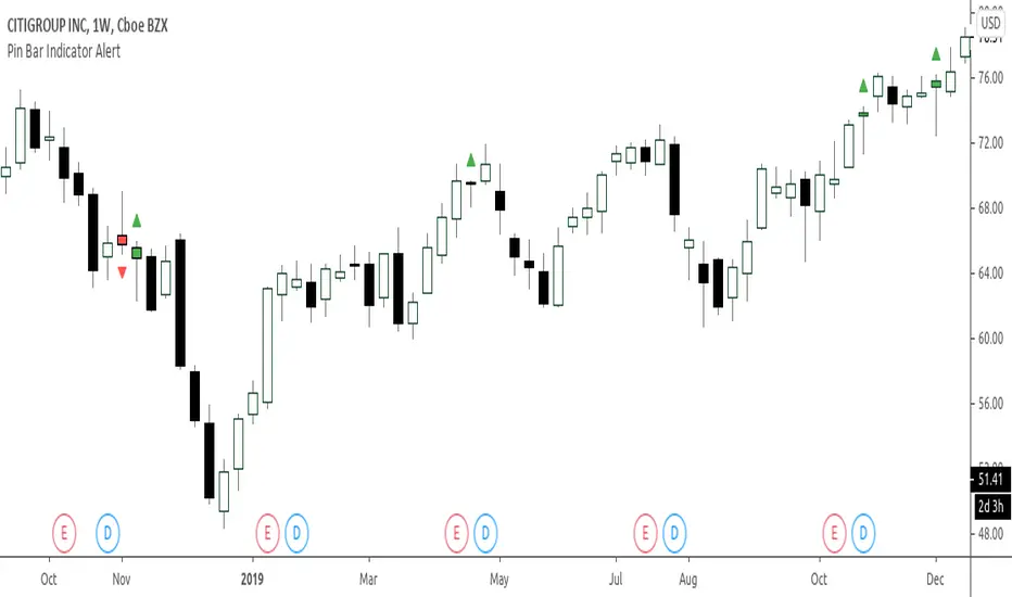
MAFIA CANDLESMafia Candles is a Exhaustion bar count and candle count indicator, Using the Leledc Candles and 1-3 counting candle play gives you a pretty good idea where a so called "top" will be or a so called "bottom" will be!
In this example, getting the transparent round circles ( either lime or red ) would mean that the move will be a good size move!
EXAMPLE=1 You see a down trend and then the Mafia Candles Flashes a Green Dot on the forming new red candle. This is where in theory you might want to consider going long on the market!
EXAMPLE=2 If you see a RED $ symbol, after a uptrend, this means in theory, there might be room for a short play or room for a small pullback in the price!
THE CIRCLES(RED OR LIME COLORED) ARE INDICATING BIGGER MOVES!
THE $ SYMBOLS (RED OR LIME COLORED) ARE INDICATING SMALLER PULLBACKS OR SMALLER PUMPS IN PRICE!
RED IS CONSIDERED TO BE A SELL!
LIME COLOR IS CONSIDERED TO BE A BUY!
AS MUCH IS BASED OF THE 1-3 CANDLE COUNT AND THE LEDLEC CANDLE DEVIATION STRATEGY, LET ME EXPLAIN THE THEORY ON BOTH THE 1-3 CANDLE COUNT AND THE LELEDC STRATEGY I COMBINE TO BRING YOU THIS ADDITION OF THE INDICATOR....
LELEDC THEORY USAGE...
An Exhaustion Bar is a bar which signals
the exhaustion of the trend in the current direction. In other words an
exhaustion bar is “A bar of last seller” in case of a downtrend and “A bar of
last buyer”in case of an uptrend.
Having said that when a party cannot take the price further in their direction,naturally the other party comes in , takes charge and reverses the direction of the trend.
TO EASIER UNDERSTAND I GIVE YOU A EASY EXAMPLE OF WHAT AN LELEDC EXHAUSTION BAR IS...
1. A wide range bar ( a bar with
long body!!!).
2. A long wick at the bottom of
the bar and no or negligible wick at the top of the bar in case of “Bear exhaustion bar” and
a long wick at the top and no or
negligible wick at the bottom of the bar in case of
“Bull exhuation bar”!!!
3. Extreme volume and.....
4. Bar forming at a key support or resistance
area including a Round Number (RN) and Big Round Number ( BRN ).THE PSYCHOLOGY BEHIND THIS!!!
Now let's assume that we have a group
of people,say 100 people who decides to go for a casual running. After running for few KM's few of
them will say “I am exhausted. I cannot run further”. They will quit running.
After running further, another bunch of runners will say “I am exhausted. I can’t run
further” and they also will quit running.
This goes on and on and then there will be a stage where only few will be left in the running. Now a stage will come where the last person left in the running will say “I
am exhausted” and he stops running. That means no one is left now in the
running.This means all are exhausted in the running.
The same way an exhaustion bar works and if we can figure out that
exhaustion bar with all the tools available on hand, we will be in a big trade
for sure!!.The reason is an exhaustion bar is formed at exact tops and bottoms most of the times.In forex with wide variety of pairs available at the counter ,one can trade this technique to make lifetime gains.
NOW LET ME EXPLAIN THE 1-3 CANDLE CORRECTION COUNT THEORY WHICH IS USED TO GET THE SUM UP SIGNALS FROM THIS INDICATOR FROM ITS INPUT LEVELS!!!
1-3 CANDLES....
The 1-3 Candlestick pattern is basically like sequential, aka a candle counting system!
1-3 CANDLE COUNT means you count the number of bullish=green candles or the bearish=red candles!
3 BULL/GREEN CANDLES in a row, each closing its close higher than the previous one before it is the 1-3 candle top count idea!
lets say you get 3 red bear candles, each candle after the first closes its body below the previous red candle before it, then you see 3 red candles with each closing lower bodies lower than the previous candle, THATS A POSSIBLE SIGN OF BEARISH EXHAUSTION, AND YOU MIGHT HAVE SOME BULLS STEP IN TO TAKE THE PRICE UP AFTER THE IMMEDIATE DOWNFALL OF THOSE 3 RED CANDLES!!
PLEASE IF ANYONE HAS QUESTIONS OR NEEDS ANY FURTHER EXPLANATION, DONT HESISITATE TO MESSAGE ME! CHALRES KNIGHT IS THE ORIGINAL AUTHOR OF THE 1-3 CANDLE COUNT AND THE LELEDC EXHAUSTION BAR INDICATOR ON METE-TRADER! R.IP CHARLES F KNIGHT!!! WE LOVE YOU AND MISS YOU BROTHER!
CHARLES KNIGHT PASSED DOWN ALL OF HIS INDICATORS AND SCRIPTS IN ORIGINAL CODE TO MYSELF WHEN HE PASSED AWAY AND I WILL CONTINUE TO HONOR HIS MEMORY BY ENHANCING HIS ORIGINAL SOURCE CODED SCRIPTS TO ENHANCE THE LIFE FOR ALL TRADERS!
CHARLIE LOVED WHEN I WOULD PUT MY OWN SWING ON HIS INDICATORS! HE TAUGHT ME EVERYTHING I KNOW AND I KNOW ONE DAY I WILL SEE HIM AGAIN!
TRADE IN PARADISE CHARLIE!!!
THE BEST TRADER IN THE WORLD!!!
在腳本中搜尋"bar"
Tensor Market Analysis Engine (TMAE)# Tensor Market Analysis Engine (TMAE)
## Advanced Multi-Dimensional Mathematical Analysis System
*Where Quantum Mathematics Meets Market Structure*
---
## 🎓 THEORETICAL FOUNDATION
The Tensor Market Analysis Engine represents a revolutionary synthesis of three cutting-edge mathematical frameworks that have never before been combined for comprehensive market analysis. This indicator transcends traditional technical analysis by implementing advanced mathematical concepts from quantum mechanics, information theory, and fractal geometry.
### 🌊 Multi-Dimensional Volatility with Jump Detection
**Hawkes Process Implementation:**
The TMAE employs a sophisticated Hawkes process approximation for detecting self-exciting market jumps. Unlike traditional volatility measures that treat price movements as independent events, the Hawkes process recognizes that market shocks cluster and exhibit memory effects.
**Mathematical Foundation:**
```
Intensity λ(t) = μ + Σ α(t - Tᵢ)
```
Where market jumps at times Tᵢ increase the probability of future jumps through the decay function α, controlled by the Hawkes Decay parameter (0.5-0.99).
**Mahalanobis Distance Calculation:**
The engine calculates volatility jumps using multi-dimensional Mahalanobis distance across up to 5 volatility dimensions:
- **Dimension 1:** Price volatility (standard deviation of returns)
- **Dimension 2:** Volume volatility (normalized volume fluctuations)
- **Dimension 3:** Range volatility (high-low spread variations)
- **Dimension 4:** Correlation volatility (price-volume relationship changes)
- **Dimension 5:** Microstructure volatility (intrabar positioning analysis)
This creates a volatility state vector that captures market behavior impossible to detect with traditional single-dimensional approaches.
### 📐 Hurst Exponent Regime Detection
**Fractal Market Hypothesis Integration:**
The TMAE implements advanced Rescaled Range (R/S) analysis to calculate the Hurst exponent in real-time, providing dynamic regime classification:
- **H > 0.6:** Trending (persistent) markets - momentum strategies optimal
- **H < 0.4:** Mean-reverting (anti-persistent) markets - contrarian strategies optimal
- **H ≈ 0.5:** Random walk markets - breakout strategies preferred
**Adaptive R/S Analysis:**
Unlike static implementations, the TMAE uses adaptive windowing that adjusts to market conditions:
```
H = log(R/S) / log(n)
```
Where R is the range of cumulative deviations and S is the standard deviation over period n.
**Dynamic Regime Classification:**
The system employs hysteresis to prevent regime flipping, requiring sustained Hurst values before regime changes are confirmed. This prevents false signals during transitional periods.
### 🔄 Transfer Entropy Analysis
**Information Flow Quantification:**
Transfer entropy measures the directional flow of information between price and volume, revealing lead-lag relationships that indicate future price movements:
```
TE(X→Y) = Σ p(yₜ₊₁, yₜ, xₜ) log
```
**Causality Detection:**
- **Volume → Price:** Indicates accumulation/distribution phases
- **Price → Volume:** Suggests retail participation or momentum chasing
- **Balanced Flow:** Market equilibrium or transition periods
The system analyzes multiple lag periods (2-20 bars) to capture both immediate and structural information flows.
---
## 🔧 COMPREHENSIVE INPUT SYSTEM
### Core Parameters Group
**Primary Analysis Window (10-100, Default: 50)**
The fundamental lookback period affecting all calculations. Optimization by timeframe:
- **1-5 minute charts:** 20-30 (rapid adaptation to micro-movements)
- **15 minute-1 hour:** 30-50 (balanced responsiveness and stability)
- **4 hour-daily:** 50-100 (smooth signals, reduced noise)
- **Asset-specific:** Cryptocurrency 20-35, Stocks 35-50, Forex 40-60
**Signal Sensitivity (0.1-2.0, Default: 0.7)**
Master control affecting all threshold calculations:
- **Conservative (0.3-0.6):** High-quality signals only, fewer false positives
- **Balanced (0.7-1.0):** Optimal risk-reward ratio for most trading styles
- **Aggressive (1.1-2.0):** Maximum signal frequency, requires careful filtering
**Signal Generation Mode:**
- **Aggressive:** Any component signals (highest frequency)
- **Confluence:** 2+ components agree (balanced approach)
- **Conservative:** All 3 components align (highest quality)
### Volatility Jump Detection Group
**Volatility Dimensions (2-5, Default: 3)**
Determines the mathematical space complexity:
- **2D:** Price + Volume volatility (suitable for clean markets)
- **3D:** + Range volatility (optimal for most conditions)
- **4D:** + Correlation volatility (advanced multi-asset analysis)
- **5D:** + Microstructure volatility (maximum sensitivity)
**Jump Detection Threshold (1.5-4.0σ, Default: 3.0σ)**
Standard deviations required for volatility jump classification:
- **Cryptocurrency:** 2.0-2.5σ (naturally volatile)
- **Stock Indices:** 2.5-3.0σ (moderate volatility)
- **Forex Major Pairs:** 3.0-3.5σ (typically stable)
- **Commodities:** 2.0-3.0σ (varies by commodity)
**Jump Clustering Decay (0.5-0.99, Default: 0.85)**
Hawkes process memory parameter:
- **0.5-0.7:** Fast decay (jumps treated as independent)
- **0.8-0.9:** Moderate clustering (realistic market behavior)
- **0.95-0.99:** Strong clustering (crisis/event-driven markets)
### Hurst Exponent Analysis Group
**Calculation Method Options:**
- **Classic R/S:** Original Rescaled Range (fast, simple)
- **Adaptive R/S:** Dynamic windowing (recommended for trading)
- **DFA:** Detrended Fluctuation Analysis (best for noisy data)
**Trending Threshold (0.55-0.8, Default: 0.60)**
Hurst value defining persistent market behavior:
- **0.55-0.60:** Weak trend persistence
- **0.65-0.70:** Clear trending behavior
- **0.75-0.80:** Strong momentum regimes
**Mean Reversion Threshold (0.2-0.45, Default: 0.40)**
Hurst value defining anti-persistent behavior:
- **0.35-0.45:** Weak mean reversion
- **0.25-0.35:** Clear ranging behavior
- **0.15-0.25:** Strong reversion tendency
### Transfer Entropy Parameters Group
**Information Flow Analysis:**
- **Price-Volume:** Classic flow analysis for accumulation/distribution
- **Price-Volatility:** Risk flow analysis for sentiment shifts
- **Multi-Timeframe:** Cross-timeframe causality detection
**Maximum Lag (2-20, Default: 5)**
Causality detection window:
- **2-5 bars:** Immediate causality (scalping)
- **5-10 bars:** Short-term flow (day trading)
- **10-20 bars:** Structural flow (swing trading)
**Significance Threshold (0.05-0.3, Default: 0.15)**
Minimum entropy for signal generation:
- **0.05-0.10:** Detect subtle information flows
- **0.10-0.20:** Clear causality only
- **0.20-0.30:** Very strong flows only
---
## 🎨 ADVANCED VISUAL SYSTEM
### Tensor Volatility Field Visualization
**Five-Layer Resonance Bands:**
The tensor field creates dynamic support/resistance zones that expand and contract based on mathematical field strength:
- **Core Layer (Purple):** Primary tensor field with highest intensity
- **Layer 2 (Neutral):** Secondary mathematical resonance
- **Layer 3 (Info Blue):** Tertiary harmonic frequencies
- **Layer 4 (Warning Gold):** Outer field boundaries
- **Layer 5 (Success Green):** Maximum field extension
**Field Strength Calculation:**
```
Field Strength = min(3.0, Mahalanobis Distance × Tensor Intensity)
```
The field amplitude adjusts to ATR and mathematical distance, creating dynamic zones that respond to market volatility.
**Radiation Line Network:**
During active tensor states, the system projects directional radiation lines showing field energy distribution:
- **8 Directional Rays:** Complete angular coverage
- **Tapering Segments:** Progressive transparency for natural visual flow
- **Pulse Effects:** Enhanced visualization during volatility jumps
### Dimensional Portal System
**Portal Mathematics:**
Dimensional portals visualize regime transitions using category theory principles:
- **Green Portals (◉):** Trending regime detection (appear below price for support)
- **Red Portals (◎):** Mean-reverting regime (appear above price for resistance)
- **Yellow Portals (○):** Random walk regime (neutral positioning)
**Tensor Trail Effects:**
Each portal generates 8 trailing particles showing mathematical momentum:
- **Large Particles (●):** Strong mathematical signal
- **Medium Particles (◦):** Moderate signal strength
- **Small Particles (·):** Weak signal continuation
- **Micro Particles (˙):** Signal dissipation
### Information Flow Streams
**Particle Stream Visualization:**
Transfer entropy creates flowing particle streams indicating information direction:
- **Upward Streams:** Volume leading price (accumulation phases)
- **Downward Streams:** Price leading volume (distribution phases)
- **Stream Density:** Proportional to information flow strength
**15-Particle Evolution:**
Each stream contains 15 particles with progressive sizing and transparency, creating natural flow visualization that makes information transfer immediately apparent.
### Fractal Matrix Grid System
**Multi-Timeframe Fractal Levels:**
The system calculates and displays fractal highs/lows across five Fibonacci periods:
- **8-Period:** Short-term fractal structure
- **13-Period:** Intermediate-term patterns
- **21-Period:** Primary swing levels
- **34-Period:** Major structural levels
- **55-Period:** Long-term fractal boundaries
**Triple-Layer Visualization:**
Each fractal level uses three-layer rendering:
- **Shadow Layer:** Widest, darkest foundation (width 5)
- **Glow Layer:** Medium white core line (width 3)
- **Tensor Layer:** Dotted mathematical overlay (width 1)
**Intelligent Labeling System:**
Smart spacing prevents label overlap using ATR-based minimum distances. Labels include:
- **Fractal Period:** Time-based identification
- **Topological Class:** Mathematical complexity rating (0, I, II, III)
- **Price Level:** Exact fractal price
- **Mahalanobis Distance:** Current mathematical field strength
- **Hurst Exponent:** Current regime classification
- **Anomaly Indicators:** Visual strength representations (○ ◐ ● ⚡)
### Wick Pressure Analysis
**Rejection Level Mathematics:**
The system analyzes candle wick patterns to project future pressure zones:
- **Upper Wick Analysis:** Identifies selling pressure and resistance zones
- **Lower Wick Analysis:** Identifies buying pressure and support zones
- **Pressure Projection:** Extends lines forward based on mathematical probability
**Multi-Layer Glow Effects:**
Wick pressure lines use progressive transparency (1-8 layers) creating natural glow effects that make pressure zones immediately visible without cluttering the chart.
### Enhanced Regime Background
**Dynamic Intensity Mapping:**
Background colors reflect mathematical regime strength:
- **Deep Transparency (98% alpha):** Subtle regime indication
- **Pulse Intensity:** Based on regime strength calculation
- **Color Coding:** Green (trending), Red (mean-reverting), Neutral (random)
**Smoothing Integration:**
Regime changes incorporate 10-bar smoothing to prevent background flicker while maintaining responsiveness to genuine regime shifts.
### Color Scheme System
**Six Professional Themes:**
- **Dark (Default):** Professional trading environment optimization
- **Light:** High ambient light conditions
- **Classic:** Traditional technical analysis appearance
- **Neon:** High-contrast visibility for active trading
- **Neutral:** Minimal distraction focus
- **Bright:** Maximum visibility for complex setups
Each theme maintains mathematical accuracy while optimizing visual clarity for different trading environments and personal preferences.
---
## 📊 INSTITUTIONAL-GRADE DASHBOARD
### Tensor Field Status Section
**Field Strength Display:**
Real-time Mahalanobis distance calculation with dynamic emoji indicators:
- **⚡ (Lightning):** Extreme field strength (>1.5× threshold)
- **● (Solid Circle):** Strong field activity (>1.0× threshold)
- **○ (Open Circle):** Normal field state
**Signal Quality Rating:**
Democratic algorithm assessment:
- **ELITE:** All 3 components aligned (highest probability)
- **STRONG:** 2 components aligned (good probability)
- **GOOD:** 1 component active (moderate probability)
- **WEAK:** No clear component signals
**Threshold and Anomaly Monitoring:**
- **Threshold Display:** Current mathematical threshold setting
- **Anomaly Level (0-100%):** Combined volatility and volume spike measurement
- **>70%:** High anomaly (red warning)
- **30-70%:** Moderate anomaly (orange caution)
- **<30%:** Normal conditions (green confirmation)
### Tensor State Analysis Section
**Mathematical State Classification:**
- **↑ BULL (Tensor State +1):** Trending regime with bullish bias
- **↓ BEAR (Tensor State -1):** Mean-reverting regime with bearish bias
- **◈ SUPER (Tensor State 0):** Random walk regime (neutral)
**Visual State Gauge:**
Five-circle progression showing tensor field polarity:
- **🟢🟢🟢⚪⚪:** Strong bullish mathematical alignment
- **⚪⚪🟡⚪⚪:** Neutral/transitional state
- **⚪⚪🔴🔴🔴:** Strong bearish mathematical alignment
**Trend Direction and Phase Analysis:**
- **📈 BULL / 📉 BEAR / ➡️ NEUTRAL:** Primary trend classification
- **🌪️ CHAOS:** Extreme information flow (>2.0 flow strength)
- **⚡ ACTIVE:** Strong information flow (1.0-2.0 flow strength)
- **😴 CALM:** Low information flow (<1.0 flow strength)
### Trading Signals Section
**Real-Time Signal Status:**
- **🟢 ACTIVE / ⚪ INACTIVE:** Long signal availability
- **🔴 ACTIVE / ⚪ INACTIVE:** Short signal availability
- **Components (X/3):** Active algorithmic components
- **Mode Display:** Current signal generation mode
**Signal Strength Visualization:**
Color-coded component count:
- **Green:** 3/3 components (maximum confidence)
- **Aqua:** 2/3 components (good confidence)
- **Orange:** 1/3 components (moderate confidence)
- **Gray:** 0/3 components (no signals)
### Performance Metrics Section
**Win Rate Monitoring:**
Estimated win rates based on signal quality with emoji indicators:
- **🔥 (Fire):** ≥60% estimated win rate
- **👍 (Thumbs Up):** 45-59% estimated win rate
- **⚠️ (Warning):** <45% estimated win rate
**Mathematical Metrics:**
- **Hurst Exponent:** Real-time fractal dimension (0.000-1.000)
- **Information Flow:** Volume/price leading indicators
- **📊 VOL:** Volume leading price (accumulation/distribution)
- **💰 PRICE:** Price leading volume (momentum/speculation)
- **➖ NONE:** Balanced information flow
- **Volatility Classification:**
- **🔥 HIGH:** Above 1.5× jump threshold
- **📊 NORM:** Normal volatility range
- **😴 LOW:** Below 0.5× jump threshold
### Market Structure Section (Large Dashboard)
**Regime Classification:**
- **📈 TREND:** Hurst >0.6, momentum strategies optimal
- **🔄 REVERT:** Hurst <0.4, contrarian strategies optimal
- **🎲 RANDOM:** Hurst ≈0.5, breakout strategies preferred
**Mathematical Field Analysis:**
- **Dimensions:** Current volatility space complexity (2D-5D)
- **Hawkes λ (Lambda):** Self-exciting jump intensity (0.00-1.00)
- **Jump Status:** 🚨 JUMP (active) / ✅ NORM (normal)
### Settings Summary Section (Large Dashboard)
**Active Configuration Display:**
- **Sensitivity:** Current master sensitivity setting
- **Lookback:** Primary analysis window
- **Theme:** Active color scheme
- **Method:** Hurst calculation method (Classic R/S, Adaptive R/S, DFA)
**Dashboard Sizing Options:**
- **Small:** Essential metrics only (mobile/small screens)
- **Normal:** Balanced information density (standard desktop)
- **Large:** Maximum detail (multi-monitor setups)
**Position Options:**
- **Top Right:** Standard placement (avoids price action)
- **Top Left:** Wide chart optimization
- **Bottom Right:** Recent price focus (scalping)
- **Bottom Left:** Maximum price visibility (swing trading)
---
## 🎯 SIGNAL GENERATION LOGIC
### Multi-Component Convergence System
**Component Signal Architecture:**
The TMAE generates signals through sophisticated component analysis rather than simple threshold crossing:
**Volatility Component:**
- **Jump Detection:** Mahalanobis distance threshold breach
- **Hawkes Intensity:** Self-exciting process activation (>0.2)
- **Multi-dimensional:** Considers all volatility dimensions simultaneously
**Hurst Regime Component:**
- **Trending Markets:** Price above SMA-20 with positive momentum
- **Mean-Reverting Markets:** Price at Bollinger Band extremes
- **Random Markets:** Bollinger squeeze breakouts with directional confirmation
**Transfer Entropy Component:**
- **Volume Leadership:** Information flow from volume to price
- **Volume Spike:** Volume 110%+ above 20-period average
- **Flow Significance:** Above entropy threshold with directional bias
### Democratic Signal Weighting
**Signal Mode Implementation:**
- **Aggressive Mode:** Any single component triggers signal
- **Confluence Mode:** Minimum 2 components must agree
- **Conservative Mode:** All 3 components must align
**Momentum Confirmation:**
All signals require momentum confirmation:
- **Long Signals:** RSI >50 AND price >EMA-9
- **Short Signals:** RSI <50 AND price 0.6):**
- **Increase Sensitivity:** Catch momentum continuation
- **Lower Mean Reversion Threshold:** Avoid counter-trend signals
- **Emphasize Volume Leadership:** Institutional accumulation/distribution
- **Tensor Field Focus:** Use expansion for trend continuation
- **Signal Mode:** Aggressive or Confluence for trend following
**Range-Bound Markets (Hurst <0.4):**
- **Decrease Sensitivity:** Avoid false breakouts
- **Lower Trending Threshold:** Quick regime recognition
- **Focus on Price Leadership:** Retail sentiment extremes
- **Fractal Grid Emphasis:** Support/resistance trading
- **Signal Mode:** Conservative for high-probability reversals
**Volatile Markets (High Jump Frequency):**
- **Increase Hawkes Decay:** Recognize event clustering
- **Higher Jump Threshold:** Avoid noise signals
- **Maximum Dimensions:** Capture full volatility complexity
- **Reduce Position Sizing:** Risk management adaptation
- **Enhanced Visuals:** Maximum information for rapid decisions
**Low Volatility Markets (Low Jump Frequency):**
- **Decrease Jump Threshold:** Capture subtle movements
- **Lower Hawkes Decay:** Treat moves as independent
- **Reduce Dimensions:** Simplify analysis
- **Increase Position Sizing:** Capitalize on compressed volatility
- **Minimal Visuals:** Reduce distraction in quiet markets
---
## 🚀 ADVANCED TRADING STRATEGIES
### The Mathematical Convergence Method
**Entry Protocol:**
1. **Fractal Grid Approach:** Monitor price approaching significant fractal levels
2. **Tensor Field Confirmation:** Verify field expansion supporting direction
3. **Portal Signal:** Wait for dimensional portal appearance
4. **ELITE/STRONG Quality:** Only trade highest quality mathematical signals
5. **Component Consensus:** Confirm 2+ components agree in Confluence mode
**Example Implementation:**
- Price approaching 21-period fractal high
- Tensor field expanding upward (bullish mathematical alignment)
- Green portal appears below price (trending regime confirmation)
- ELITE quality signal with 3/3 components active
- Enter long position with stop below fractal level
**Risk Management:**
- **Stop Placement:** Below/above fractal level that generated signal
- **Position Sizing:** Based on Mahalanobis distance (higher distance = smaller size)
- **Profit Targets:** Next fractal level or tensor field resistance
### The Regime Transition Strategy
**Regime Change Detection:**
1. **Monitor Hurst Exponent:** Watch for persistent moves above/below thresholds
2. **Portal Color Change:** Regime transitions show different portal colors
3. **Background Intensity:** Increasing regime background intensity
4. **Mathematical Confirmation:** Wait for regime confirmation (hysteresis)
**Trading Implementation:**
- **Trending Transitions:** Trade momentum breakouts, follow trend
- **Mean Reversion Transitions:** Trade range boundaries, fade extremes
- **Random Transitions:** Trade breakouts with tight stops
**Advanced Techniques:**
- **Multi-Timeframe:** Confirm regime on higher timeframe
- **Early Entry:** Enter on regime transition rather than confirmation
- **Regime Strength:** Larger positions during strong regime signals
### The Information Flow Momentum Strategy
**Flow Detection Protocol:**
1. **Monitor Transfer Entropy:** Watch for significant information flow shifts
2. **Volume Leadership:** Strong edge when volume leads price
3. **Flow Acceleration:** Increasing flow strength indicates momentum
4. **Directional Confirmation:** Ensure flow aligns with intended trade direction
**Entry Signals:**
- **Volume → Price Flow:** Enter during accumulation/distribution phases
- **Price → Volume Flow:** Enter on momentum confirmation breaks
- **Flow Reversal:** Counter-trend entries when flow reverses
**Optimization:**
- **Scalping:** Use immediate flow detection (2-5 bar lag)
- **Swing Trading:** Use structural flow (10-20 bar lag)
- **Multi-Asset:** Compare flow between correlated assets
### The Tensor Field Expansion Strategy
**Field Mathematics:**
The tensor field expansion indicates mathematical pressure building in market structure:
**Expansion Phases:**
1. **Compression:** Field contracts, volatility decreases
2. **Tension Building:** Mathematical pressure accumulates
3. **Expansion:** Field expands rapidly with directional movement
4. **Resolution:** Field stabilizes at new equilibrium
**Trading Applications:**
- **Compression Trading:** Prepare for breakout during field contraction
- **Expansion Following:** Trade direction of field expansion
- **Reversion Trading:** Fade extreme field expansion
- **Multi-Dimensional:** Consider all field layers for confirmation
### The Hawkes Process Event Strategy
**Self-Exciting Jump Trading:**
Understanding that market shocks cluster and create follow-on opportunities:
**Jump Sequence Analysis:**
1. **Initial Jump:** First volatility jump detected
2. **Clustering Phase:** Hawkes intensity remains elevated
3. **Follow-On Opportunities:** Additional jumps more likely
4. **Decay Period:** Intensity gradually decreases
**Implementation:**
- **Jump Confirmation:** Wait for mathematical jump confirmation
- **Direction Assessment:** Use other components for direction
- **Clustering Trades:** Trade subsequent moves during high intensity
- **Decay Exit:** Exit positions as Hawkes intensity decays
### The Fractal Confluence System
**Multi-Timeframe Fractal Analysis:**
Combining fractal levels across different periods for high-probability zones:
**Confluence Zones:**
- **Double Confluence:** 2 fractal levels align
- **Triple Confluence:** 3+ fractal levels cluster
- **Mathematical Confirmation:** Tensor field supports the level
- **Information Flow:** Transfer entropy confirms direction
**Trading Protocol:**
1. **Identify Confluence:** Find 2+ fractal levels within 1 ATR
2. **Mathematical Support:** Verify tensor field alignment
3. **Signal Quality:** Wait for STRONG or ELITE signal
4. **Risk Definition:** Use fractal level for stop placement
5. **Profit Targeting:** Next major fractal confluence zone
---
## ⚠️ COMPREHENSIVE RISK MANAGEMENT
### Mathematical Position Sizing
**Mahalanobis Distance Integration:**
Position size should inversely correlate with mathematical field strength:
```
Position Size = Base Size × (Threshold / Mahalanobis Distance)
```
**Risk Scaling Matrix:**
- **Low Field Strength (<2.0):** Standard position sizing
- **Moderate Field Strength (2.0-3.0):** 75% position sizing
- **High Field Strength (3.0-4.0):** 50% position sizing
- **Extreme Field Strength (>4.0):** 25% position sizing or no trade
### Signal Quality Risk Adjustment
**Quality-Based Position Sizing:**
- **ELITE Signals:** 100% of planned position size
- **STRONG Signals:** 75% of planned position size
- **GOOD Signals:** 50% of planned position size
- **WEAK Signals:** No position or paper trading only
**Component Agreement Scaling:**
- **3/3 Components:** Full position size
- **2/3 Components:** 75% position size
- **1/3 Components:** 50% position size or skip trade
### Regime-Adaptive Risk Management
**Trending Market Risk:**
- **Wider Stops:** Allow for trend continuation
- **Trend Following:** Trade with regime direction
- **Higher Position Size:** Trend probability advantage
- **Momentum Stops:** Trail stops based on momentum indicators
**Mean-Reverting Market Risk:**
- **Tighter Stops:** Quick exits on trend continuation
- **Contrarian Positioning:** Trade against extremes
- **Smaller Position Size:** Higher reversal failure rate
- **Level-Based Stops:** Use fractal levels for stops
**Random Market Risk:**
- **Breakout Focus:** Trade only clear breakouts
- **Tight Initial Stops:** Quick exit if breakout fails
- **Reduced Frequency:** Skip marginal setups
- **Range-Based Targets:** Profit targets at range boundaries
### Volatility-Adaptive Risk Controls
**High Volatility Periods:**
- **Reduced Position Size:** Account for wider price swings
- **Wider Stops:** Avoid noise-based exits
- **Lower Frequency:** Skip marginal setups
- **Faster Exits:** Take profits more quickly
**Low Volatility Periods:**
- **Standard Position Size:** Normal risk parameters
- **Tighter Stops:** Take advantage of compressed ranges
- **Higher Frequency:** Trade more setups
- **Extended Targets:** Allow for compressed volatility expansion
### Multi-Timeframe Risk Alignment
**Higher Timeframe Trend:**
- **With Trend:** Standard or increased position size
- **Against Trend:** Reduced position size or skip
- **Neutral Trend:** Standard position size with tight management
**Risk Hierarchy:**
1. **Primary:** Current timeframe signal quality
2. **Secondary:** Higher timeframe trend alignment
3. **Tertiary:** Mathematical field strength
4. **Quaternary:** Market regime classification
---
## 📚 EDUCATIONAL VALUE AND MATHEMATICAL CONCEPTS
### Advanced Mathematical Concepts
**Tensor Analysis in Markets:**
The TMAE introduces traders to tensor analysis, a branch of mathematics typically reserved for physics and advanced engineering. Tensors provide a framework for understanding multi-dimensional market relationships that scalar and vector analysis cannot capture.
**Information Theory Applications:**
Transfer entropy implementation teaches traders about information flow in markets, a concept from information theory that quantifies directional causality between variables. This provides intuition about market microstructure and participant behavior.
**Fractal Geometry in Trading:**
The Hurst exponent calculation exposes traders to fractal geometry concepts, helping understand that markets exhibit self-similar patterns across multiple timeframes. This mathematical insight transforms how traders view market structure.
**Stochastic Process Theory:**
The Hawkes process implementation introduces concepts from stochastic process theory, specifically self-exciting point processes. This provides mathematical framework for understanding why market events cluster and exhibit memory effects.
### Learning Progressive Complexity
**Beginner Mathematical Concepts:**
- **Volatility Dimensions:** Understanding multi-dimensional analysis
- **Regime Classification:** Learning market personality types
- **Signal Democracy:** Algorithmic consensus building
- **Visual Mathematics:** Interpreting mathematical concepts visually
**Intermediate Mathematical Applications:**
- **Mahalanobis Distance:** Statistical distance in multi-dimensional space
- **Rescaled Range Analysis:** Fractal dimension measurement
- **Information Entropy:** Quantifying uncertainty and causality
- **Field Theory:** Understanding mathematical fields in market context
**Advanced Mathematical Integration:**
- **Tensor Field Dynamics:** Multi-dimensional market force analysis
- **Stochastic Self-Excitation:** Event clustering and memory effects
- **Categorical Composition:** Mathematical signal combination theory
- **Topological Market Analysis:** Understanding market shape and connectivity
### Practical Mathematical Intuition
**Developing Market Mathematics Intuition:**
The TMAE serves as a bridge between abstract mathematical concepts and practical trading applications. Traders develop intuitive understanding of:
- **How markets exhibit mathematical structure beneath apparent randomness**
- **Why multi-dimensional analysis reveals patterns invisible to single-variable approaches**
- **How information flows through markets in measurable, predictable ways**
- **Why mathematical models provide probabilistic edges rather than certainties**
---
## 🔬 IMPLEMENTATION AND OPTIMIZATION
### Getting Started Protocol
**Phase 1: Observation (Week 1)**
1. **Apply with defaults:** Use standard settings on your primary trading timeframe
2. **Study visual elements:** Learn to interpret tensor fields, portals, and streams
3. **Monitor dashboard:** Observe how metrics change with market conditions
4. **No trading:** Focus entirely on pattern recognition and understanding
**Phase 2: Pattern Recognition (Week 2-3)**
1. **Identify signal patterns:** Note what market conditions produce different signal qualities
2. **Regime correlation:** Observe how Hurst regimes affect signal performance
3. **Visual confirmation:** Learn to read tensor field expansion and portal signals
4. **Component analysis:** Understand which components drive signals in different markets
**Phase 3: Parameter Optimization (Week 4-5)**
1. **Asset-specific tuning:** Adjust parameters for your specific trading instrument
2. **Timeframe optimization:** Fine-tune for your preferred trading timeframe
3. **Sensitivity adjustment:** Balance signal frequency with quality
4. **Visual customization:** Optimize colors and intensity for your trading environment
**Phase 4: Live Implementation (Week 6+)**
1. **Paper trading:** Test signals with hypothetical trades
2. **Small position sizing:** Begin with minimal risk during learning phase
3. **Performance tracking:** Monitor actual vs. expected signal performance
4. **Continuous optimization:** Refine settings based on real performance data
### Performance Monitoring System
**Signal Quality Tracking:**
- **ELITE Signal Win Rate:** Track highest quality signals separately
- **Component Performance:** Monitor which components provide best signals
- **Regime Performance:** Analyze performance across different market regimes
- **Timeframe Analysis:** Compare performance across different session times
**Mathematical Metric Correlation:**
- **Field Strength vs. Performance:** Higher field strength should correlate with better performance
- **Component Agreement vs. Win Rate:** More component agreement should improve win rates
- **Regime Alignment vs. Success:** Trading with mathematical regime should outperform
### Continuous Optimization Process
**Monthly Review Protocol:**
1. **Performance Analysis:** Review win rates, profit factors, and maximum drawdown
2. **Parameter Assessment:** Evaluate if current settings remain optimal
3. **Market Adaptation:** Adjust for changes in market character or volatility
4. **Component Weighting:** Consider if certain components should receive more/less emphasis
**Quarterly Deep Analysis:**
1. **Mathematical Model Validation:** Verify that mathematical relationships remain valid
2. **Regime Distribution:** Analyze time spent in different market regimes
3. **Signal Evolution:** Track how signal characteristics change over time
4. **Correlation Analysis:** Monitor correlations between different mathematical components
---
## 🌟 UNIQUE INNOVATIONS AND CONTRIBUTIONS
### Revolutionary Mathematical Integration
**First-Ever Implementations:**
1. **Multi-Dimensional Volatility Tensor:** First indicator to implement true tensor analysis for market volatility
2. **Real-Time Hawkes Process:** First trading implementation of self-exciting point processes
3. **Transfer Entropy Trading Signals:** First practical application of information theory for trade generation
4. **Democratic Component Voting:** First algorithmic consensus system for signal generation
5. **Fractal-Projected Signal Quality:** First system to predict signal quality at future price levels
### Advanced Visualization Innovations
**Mathematical Visualization Breakthroughs:**
- **Tensor Field Radiation:** Visual representation of mathematical field energy
- **Dimensional Portal System:** Category theory visualization for regime transitions
- **Information Flow Streams:** Real-time visual display of market information transfer
- **Multi-Layer Fractal Grid:** Intelligent spacing and projection system
- **Regime Intensity Mapping:** Dynamic background showing mathematical regime strength
### Practical Trading Innovations
**Trading System Advances:**
- **Quality-Weighted Signal Generation:** Signals rated by mathematical confidence
- **Regime-Adaptive Strategy Selection:** Automatic strategy optimization based on market personality
- **Anti-Spam Signal Protection:** Mathematical prevention of signal clustering
- **Component Performance Tracking:** Real-time monitoring of algorithmic component success
- **Field-Strength Position Sizing:** Mathematical volatility integration for risk management
---
## ⚖️ RESPONSIBLE USAGE AND LIMITATIONS
### Mathematical Model Limitations
**Understanding Model Boundaries:**
While the TMAE implements sophisticated mathematical concepts, traders must understand fundamental limitations:
- **Markets Are Not Purely Mathematical:** Human psychology, news events, and fundamental factors create unpredictable elements
- **Past Performance Limitations:** Mathematical relationships that worked historically may not persist indefinitely
- **Model Risk:** Complex models can fail during unprecedented market conditions
- **Overfitting Potential:** Highly optimized parameters may not generalize to future market conditions
### Proper Implementation Guidelines
**Risk Management Requirements:**
- **Never Risk More Than 2% Per Trade:** Regardless of signal quality
- **Diversification Mandatory:** Don't rely solely on mathematical signals
- **Position Sizing Discipline:** Use mathematical field strength for sizing, not confidence
- **Stop Loss Non-Negotiable:** Every trade must have predefined risk parameters
**Realistic Expectations:**
- **Mathematical Edge, Not Certainty:** The indicator provides probabilistic advantages, not guaranteed outcomes
- **Learning Curve Required:** Complex mathematical concepts require time to master
- **Market Adaptation Necessary:** Parameters must evolve with changing market conditions
- **Continuous Education Important:** Understanding underlying mathematics improves application
### Ethical Trading Considerations
**Market Impact Awareness:**
- **Information Asymmetry:** Advanced mathematical analysis may provide advantages over other market participants
- **Position Size Responsibility:** Large positions based on mathematical signals can impact market structure
- **Sharing Knowledge:** Consider educational contributions to trading community
- **Fair Market Participation:** Use mathematical advantages responsibly within market framework
### Professional Development Path
**Skill Development Sequence:**
1. **Basic Mathematical Literacy:** Understand fundamental concepts before advanced application
2. **Risk Management Mastery:** Develop disciplined risk control before relying on complex signals
3. **Market Psychology Understanding:** Combine mathematical analysis with behavioral market insights
4. **Continuous Learning:** Stay updated on mathematical finance developments and market evolution
---
## 🔮 CONCLUSION
The Tensor Market Analysis Engine represents a quantum leap forward in technical analysis, successfully bridging the gap between advanced pure mathematics and practical trading applications. By integrating multi-dimensional volatility analysis, fractal market theory, and information flow dynamics, the TMAE reveals market structure invisible to conventional analysis while maintaining visual clarity and practical usability.
### Mathematical Innovation Legacy
This indicator establishes new paradigms in technical analysis:
- **Tensor analysis for market volatility understanding**
- **Stochastic self-excitation for event clustering prediction**
- **Information theory for causality-based trade generation**
- **Democratic algorithmic consensus for signal quality enhancement**
- **Mathematical field visualization for intuitive market understanding**
### Practical Trading Revolution
Beyond mathematical innovation, the TMAE transforms practical trading:
- **Quality-rated signals replace binary buy/sell decisions**
- **Regime-adaptive strategies automatically optimize for market personality**
- **Multi-dimensional risk management integrates mathematical volatility measures**
- **Visual mathematical concepts make complex analysis immediately interpretable**
- **Educational value creates lasting improvement in trading understanding**
### Future-Proof Design
The mathematical foundations ensure lasting relevance:
- **Universal mathematical principles transcend market evolution**
- **Multi-dimensional analysis adapts to new market structures**
- **Regime detection automatically adjusts to changing market personalities**
- **Component democracy allows for future algorithmic additions**
- **Mathematical visualization scales with increasing market complexity**
### Commitment to Excellence
The TMAE represents more than an indicator—it embodies a philosophy of bringing rigorous mathematical analysis to trading while maintaining practical utility and visual elegance. Every component, from the multi-dimensional tensor fields to the democratic signal generation, reflects a commitment to mathematical accuracy, trading practicality, and educational value.
### Trading with Mathematical Precision
In an era where markets grow increasingly complex and computational, the TMAE provides traders with mathematical tools previously available only to institutional quantitative research teams. Yet unlike academic mathematical models, the TMAE translates complex concepts into intuitive visual representations and practical trading signals.
By combining the mathematical rigor of tensor analysis, the statistical power of multi-dimensional volatility modeling, and the information-theoretic insights of transfer entropy, traders gain unprecedented insight into market structure and dynamics.
### Final Perspective
Markets, like nature, exhibit profound mathematical beauty beneath apparent chaos. The Tensor Market Analysis Engine serves as a mathematical lens that reveals this hidden order, transforming how traders perceive and interact with market structure.
Through mathematical precision, visual elegance, and practical utility, the TMAE empowers traders to see beyond the noise and trade with the confidence that comes from understanding the mathematical principles governing market behavior.
Trade with mathematical insight. Trade with the power of tensors. Trade with the TMAE.
*"In mathematics, you don't understand things. You just get used to them." - John von Neumann*
*With the TMAE, mathematical market understanding becomes not just possible, but intuitive.*
— Dskyz, Trade with insight. Trade with anticipation.
DDDDD: ATR & ADR Table + Suggested Time-based Exit📈 DDDDD: ATR & ADR Table + Suggested Time-based Exit
This indicator provides a simple yet powerful table displaying key volatility metrics for any timeframe you apply it to. It is designed for traders who want to assess the volatility of an asset, estimate the average time required for a potential move, and define a time-based exit strategy.
🔍 Features:
Displays ATR (Average True Range) for the selected length
Shows Average Range (High-Low) and Maximum Range over a configurable number of bars
Calculates Avg Bars/Move → average number of bars needed to achieve the maximum range
Calculates Recommended Exit Bars → suggested maximum holding period (in bars) before considering an exit if price hasn’t moved as expected
All values dynamically adjust based on the chart’s current timeframe
Outputs values directly in a table overlay on your main chart for quick reference
📝 How to interpret the table:
Field Meaning
ATR (14) Average True Range over the last 14 bars (volatility indicator)
Avg Range (20) Average High-Low range over the last 20 bars
Max Range Maximum High-Low range observed in the last 20 bars
Avg Bars/Move Average number of bars it takes to achieve a Max Range move
Rec. Exit Bars Suggested max holding period (bars) → consider exit if move hasn’t occurred
✅ How to use:
Apply this indicator to any chart (works on minutes, hourly, daily, weekly…)
It will automatically calculate based on the chart’s current timeframe
Use ATR & Avg Range to gauge volatility
Use Avg Bars/Move to estimate how long the market usually takes to achieve a big move
Use Rec. Exit Bars as a soft stop — if price hasn’t moved by this time, consider exiting due to declining probability of a breakout
⚠️ Notes:
All values are relative to your current chart timeframe. For example:
→ On a daily chart, ATR represents daily volatility
→ On a 1H chart, ATR represents hourly volatility
“Bars” refers to the bars of the current timeframe. Always interpret time accordingly.
Perfect for traders who want to:
Time their trades based on average volatility
Avoid overholding losing positions
Set time-based exit rules to complement price-based stoplosses
EXODUS EXODUS by (DAFE) Trading Systems
EXODUS is a sophisticated trading algorithm built by Dskyz (DAFE) Trading Systems for competitive and competition purposes, designed to identify high-probability trades with robust risk management. this strategy leverages a multi-signal voting system, combining three core components—SPR, VWMO, and VEI—alongside ADX, choppiness filters, and ATR-based volatility gates to ensure trades are taken only in favorable market conditions. the algo uses a take-profit to stop-loss ratio, dynamic position sizing, and a strict voting mechanism requiring all signals to align before entering a trade.
EXODUS was not overfitted for any specific symbol. instead, it uses a generic tuned setting, making it versatile across various markets. while it can trade futures, it’s not currently set up for it but has the potential to do more with further development. visuals are intentionally minimal due to its competition focus, prioritizing performance over aesthetics. a more visually stunning version may be released in the future with enhanced graphics.
The Unique Core Components Developed for EXODUS
SPR (Session Price Recalibration)
SPR measures momentum during regular trading hours (RTH, 0930-1600, America/New_York) to catch session-specific trends.
spr_lookback = input.int(15, "SPR Lookback") this sets how many bars back SPR looks to calculate momentum (default 15 bars). it compares the current session’s price-volume score to the score 15 bars ago to gauge momentum strength.
how it works: a longer lookback smooths out the signal, focusing on bigger trends. a shorter one makes SPR more sensitive to recent moves.
how to adjust: on a 1-hour chart, 15 bars is 15 hours (about 2 trading days). if you’re on a shorter timeframe like 5 minutes, 15 bars is just 75 minutes, so you might want to increase it to 50 or 100 to capture more meaningful trends. if you’re trading a choppy stock, a shorter lookback (like 5) can help catch quick moves, but it might give more false signals.
spr_threshold = input.float (0.7, "SPR Threshold")
this is the cutoff for SPR to vote for a trade (default 0.7). if SPR’s normalized value is above 0.7, it votes for a long; below -0.7, it votes for a short.
how it works: SPR normalizes its momentum score by ATR, so this threshold ensures only strong moves count. a higher threshold means fewer trades but higher conviction.
how to adjust: if you’re getting too few trades, lower it to 0.5 to let more signals through. if you’re seeing too many false entries, raise it to 1.0 for stricter filtering. test on your chart to find a balance.
spr_atr_length = input.int(21, "SPR ATR Length") this sets the ATR period (default 21 bars) used to normalize SPR’s momentum score. ATR measures volatility, so this makes SPR’s signal relative to market conditions.
how it works: a longer ATR period (like 21) smooths out volatility, making SPR less jumpy. a shorter one makes it more reactive.
how to adjust: if you’re trading a volatile stock like TSLA, a longer period (30 or 50) can help avoid noise. for a calmer stock, try 10 to make SPR more responsive. match this to your timeframe—shorter timeframes might need a shorter ATR.
rth_session = input.session("0930-1600","SPR: RTH Sess.") rth_timezone = "America/New_York" this defines the session SPR uses (0930-1600, New York time). SPR only calculates momentum during these hours to focus on RTH activity.
how it works: it ignores pre-market or after-hours noise, ensuring SPR captures the main market action.
how to adjust: if you trade a different session (like London hours, 0300-1200 EST), change the session to match. you can also adjust the timezone if you’re in a different region, like "Europe/London". just make sure your chart’s timezone aligns with this setting.
VWMO (Volume-Weighted Momentum Oscillator)
VWMO measures momentum weighted by volume to spot sustained, high-conviction moves.
vwmo_momlen = input.int(21, "VWMO Momentum Length") this sets how many bars back VWMO looks to calculate price momentum (default 21 bars). it takes the price change (close minus close 21 bars ago).
how it works: a longer period captures bigger trends, while a shorter one reacts to recent swings.
how to adjust: on a daily chart, 21 bars is about a month—good for trend trading. on a 5-minute chart, it’s just 105 minutes, so you might bump it to 50 or 100 for more meaningful moves. if you want faster signals, drop it to 10, but expect more noise.
vwmo_volback = input.int(30, "VWMO Volume Lookback") this sets the period for calculating average volume (default 30 bars). VWMO weights momentum by volume divided by this average.
how it works: it compares current volume to the average to see if a move has strong participation. a longer lookback smooths the average, while a shorter one makes it more sensitive.
how to adjust: for stocks with spiky volume (like NVDA on earnings), a longer lookback (50 or 100) avoids overreacting to one-off spikes. for steady volume stocks, try 20. match this to your timeframe—shorter timeframes might need a shorter lookback.
vwmo_smooth = input.int(9, "VWMO Smoothing")
this sets the SMA period to smooth VWMO’s raw momentum (default 9 bars).
how it works: smoothing reduces noise in the signal, making VWMO more reliable for voting. a longer smoothing period cuts more noise but adds lag.
how to adjust: if VWMO is too jumpy (lots of false votes), increase to 15. if it’s too slow and missing trades, drop to 5. test on your chart to see what keeps the signal clean but responsive.
vwmo_threshold = input.float(10, "VWMO Threshold") this is the cutoff for VWMO to vote for a trade (default 10). above 10, it votes for a long; below -10, a short.
how it works: it ensures only strong momentum signals count. a higher threshold means fewer but stronger trades.
how to adjust: if you want more trades, lower it to 5. if you’re getting too many weak signals, raise it to 15. this depends on your market—volatile stocks might need a higher threshold to filter noise.
VEI (Velocity Efficiency Index)
VEI measures market efficiency and velocity to filter out choppy moves and focus on strong trends.
vei_eflen = input.int(14, "VEI Efficiency Smoothing") this sets the EMA period for smoothing VEI’s efficiency calc (bar range / volume, default 14 bars).
how it works: efficiency is how much price moves per unit of volume. smoothing it with an EMA reduces noise, focusing on consistent efficiency. a longer period smooths more but adds lag.
how to adjust: for choppy markets, increase to 20 to filter out noise. for faster markets, drop to 10 for quicker signals. this should match your timeframe—shorter timeframes might need a shorter period.
vei_momlen = input.int(8, "VEI Momentum Length") this sets how many bars back VEI looks to calculate momentum in efficiency (default 8 bars).
how it works: it measures the change in smoothed efficiency over 8 bars, then adjusts for inertia (volume-to-range). a longer period captures bigger shifts, while a shorter one reacts faster.
how to adjust: if VEI is missing quick reversals, drop to 5. if it’s too noisy, raise to 12. test on your chart to see what catches the right moves without too many false signals.
vei_threshold = input.float(4.5, "VEI Threshold") this is the cutoff for VEI to vote for a trade (default 4.5). above 4.5, it votes for a long; below -4.5, a short.
how it works: it ensures only strong, efficient moves count. a higher threshold means fewer trades but higher quality.
how to adjust: if you’re not getting enough trades, lower to 3. if you’re seeing too many false entries, raise to 6. this depends on your market—fast stocks like NQ1 might need a lower threshold.
Features
Multi-Signal Voting: requires all three signals (SPR, VWMO, VEI) to align for a trade, ensuring high-probability setups.
Risk Management: uses ATR-based stops (2.1x) and take-profits (4.1x), with dynamic position sizing based on a risk percentage (default 0.4%).
Market Filters: ADX (default 27) ensures trending conditions, choppiness index (default 54.5) avoids sideways markets, and ATR expansion (default 1.12) confirms volatility.
Dashboard: provides real-time stats like SPR, VWMO, VEI values, net P/L, win rate, and streak, with a clean, functional design.
Visuals
EXODUS prioritizes performance over visuals, as it was built for competitive and competition purposes. entry/exit signals are marked with simple labels and shapes, and a basic heatmap highlights market regimes. a more visually stunning update may be released later, with enhanced graphics and overlays.
Usage
EXODUS is designed for stocks and ETFs but can be adapted for futures with adjustments. it performs best in trending markets with sufficient volatility, as confirmed by its generic tuning across symbols like TSLA, AMD, NVDA, and NQ1. adjust inputs like SPR threshold, VWMO smoothing, or VEI momentum length to suit specific assets or timeframes.
Setting I used: (Again, these are a generic setting, each security needs to be fine tuned)
SPR LB = 19 SPR TH = 0.5 SPR ATR L= 21 SPR RTH Sess: 9:30 – 16:00
VWMO L = 21 VWMO LB = 18 VWMO S = 6 VWMO T = 8
VEI ES = 14 VEI ML = 21 VEI T = 4
R % = 0.4
ATR L = 21 ATR M (S) =1.1 TP Multi = 2.1 ATR min mult = 0.8 ATR Expansion = 1.02
ADX L = 21 Min ADX = 25
Choppiness Index = 14 Chop. Max T = 55.5
Backtesting: TSLA
Frame: Jan 02, 2018, 08:00 — May 01, 2025, 09:00
Slippage: 3
Commission .01
Disclaimer
this strategy is for educational purposes. past performance is not indicative of future results. trading involves significant risk, and you should only trade with capital you can afford to lose. always backtest and validate any strategy before using it in live markets.
(This publishing will most likely be taken down do to some miscellaneous rule about properly displaying charting symbols, or whatever. Once I've identified what part of the publishing they want to pick on, I'll adjust and repost.)
About the Author
Dskyz (DAFE) Trading Systems is dedicated to building high-performance trading algorithms. EXODUS is a product of rigorous research and development, aimed at delivering consistent, and data-driven trading solutions.
Use it with discipline. Use it with clarity. Trade smarter.
**I will continue to release incredible strategies and indicators until I turn this into a brand or until someone offers me a contract.
2025 Created by Dskyz, powered by DAFE Trading Systems. Trade smart, trade bold.
WhispererRealtimeVolumeLibrary "WhispererRealtimeVolume"
▮ Overview
The Whisperer Realtime Volume Library is a lightweight and reusable Pine Script® library designed for real-time volume analysis.
It calculates up, down, and neutral volumes dynamically, making it an essential tool for traders who want to gain deeper insights into market activity.
This library is a simplified and modular version of the original "Realtime Volume Bars w Market Buy/Sell/Neutral split & Mkt Delta" indicator by the_MarketWhisperer , tailored for integration into custom scripts.
How bars are classified
- Up Bars
If the current bar’s closing price is higher than the previous bar’s closing price, it is classified as an up bar.
Volume handling:
The increase in volume for this bar is added to the up volume.
This represents buying pressure.
- Down Bars
If the current bar’s closing price is lower than the previous bar’s closing price, it is classified as a down bar.
Volume handling:
The increase in volume for this bar is added to the down volume.
This represents selling pressure.
- Neutral Bars
If the current bar’s closing price is the same as the previous bar’s closing price, it is classified as a neutral bar.
Volume handling:
If neutral volume is enabled, the volume is added to the neutral volume.
If neutral volume is not enabled, the volume is assigned to the same direction as the previous bar (up or down). If the previous direction is unknown, it is added to the neutral volume.
▮ What to look for
Real-Time Volume Calculation : Analyze up, down, and neutral volumes in real-time based on price movements and bar volume.
Customizable Start Line : Add a visual reference line to your chart for better context by viewing the starting point of real-time bars.
Ease of Integration : Designed as a library for seamless use in other Pine Script® indicators or strategies.
▮ How to use
Example code:
//@version=6
indicator("Volume Realtime from Whisperer")
import andre_007/WhispererRealtimeVolume/4 as MW
MW.displayStartLine(startLineColor = color.gray, startLineWidth = 1, startLineStyle = line.style_dashed,
displayStartLine = true, y1=volume, y2=volume + 10)
= MW.mw_upDownVolumeRealtime(true)
plot(volume, style=plot.style_columns, color=color.gray)
plot(volumeUp, style=plot.style_columns, color=color.green)
plot(volumeDown, style=plot.style_columns, color=color.red)
plot(volumeNeutral, style=plot.style_columns, color=color.purple)
▮ Credits
This library is inspired by the original work of the_MarketWhisperer , whose "Realtime Volume Bars" indicator served as the foundation.
Link to original indicator :
Anchored Darvas Box## ANCHORED DARVAS BOX
---
### OVERVIEW
**Anchored Darvas Box** lets you drop a single timestamp on your chart and build a Darvas-style consolidation zone forward from that exact candle. The indicator freezes the first user-defined number of bars to establish the range, verifies that price respects that range for another user-defined number of bars, then waits for the first decisive breakout. The resulting rectangle captures every tick of the accumulation phase and the exact moment of expansion—no manual drawing, complete timestamp precision.
---
### HISTORICAL BACKGROUND
Nicolas Darvas’s 1950s box theory tracked institutional accumulation by hand-drawing rectangles around tight price ranges. A trade was triggered only when price escaped the rectangle.
The anchored version preserves Darvas’s logic but pins the entire sequence to a user-chosen candle: perfect for analysing a market open, an earnings release, FOMC minute, or any other catalytic bar.
---
### ALGORITHM DETAIL
1. **ANCHOR BAR**
*You provide a timestamp via the settings panel.* The script waits until the chart reaches that bar and records its index as **startBar**.
2. **RANGE DEFINITION — BARS 1-7**
• `rangeHigh` = highest high of bars 1-7 plus optional tolerance.
• `rangeLow` = lowest low of bars 1-7 minus optional tolerance.
3. **RANGE VALIDATION — BARS 8-14**
• Price must stay inside ` `.
• Any violation aborts the test; no box is created.
4. **ARMED STATE**
• If bars 8-14 hold the range, two live guide-lines appear:
– **Green** at `rangeHigh`
– **Red** at `rangeLow`
• The script is now “armed,” waiting indefinitely for the first true breakout.
5. **BREAKOUT & BOX CREATION**
• **Up breakout** =`high > rangeHigh` → rectangle drawn in **green**.
• **Down breakout**=`low < rangeLow` → rectangle drawn in **red**.
• Box extends from **startBar** to the breakout bar and never updates again.
• Optional labels print the dollar and percentage height of the box at its left edge.
6. **OPTIONAL COOLDOWN**
• After the box is painted the script can stay silent for a user-defined number of bars, letting you study the fallout without another range immediately arming on top of it.
---
### INPUT PARAMETERS
• **ANCHOR TIME** – Precise yyyy-mm-dd HH:MM:SS that seeds the sequence.
• **BARS TO DEFINE RANGE** – Default 7; affects both definition and validation windows.
• **OPTIONAL TOLERANCE** – Absolute price buffer to ignore micro-wicks.
• **COOLDOWN BARS AFTER BREAKOUT** – Pause length before the indicator is allowed to re-anchor (set to zero to disable).
• **SHOW BOX DISTANCE LABELS** – Toggle to print Δ\$ and Δ% on every completed box.
---
### USER WORKFLOW
1. Add the indicator, open settings, and set **ANCHOR TIME** to the candle you care about (e.g., “2025-04-23 09:30:00” for NYSE open).
2. Watch live as the script:
– Paints the seven-bar range.
– Draws validation lines.
– Locks in the box on breakout.
3. Use the box boundaries as structural stops, targets, or context for further trades.
---
### PRACTICAL APPLICATIONS
• **OPENING RANGE BREAKOUTS** – Anchor at the first second of the session; capture the initial 7-bar range and trade the first clean break.
• **EVENT STUDIES** – Anchor at a news candle to measure immediate post-event volatility.
• **VOLUME PROFILE FUSION** – Combine the anchored box with VPVR to see if the breakout occurs at a high-volume node or a low-liquidity pocket.
• **RISK DISCIPLINE** – Stop-loss can sit just inside the opposite edge of the anchored range, enforcing objective risk.
---
### ADVANCED CUSTOMISATION IDEAS
• **MULTIPLE ANCHORS** – Clone the indicator and anchor several boxes (e.g., London open, New York open).
• **DYNAMIC WINDOW** – Switch the 7-bar fixed length to a volatility-scaled length (ATR percentile).
• **STRATEGY WRAPPER** – Turn the indicator into a `strategy{}` script and back-test anchored boxes on decades of data.
---
### FINAL THOUGHTS
Anchored Darvas Boxes give you Darvas’s timeless range-break methodology anchored to any candle of interest—perfect for dissecting openings, economic releases, or your own bespoke “important” bars with laboratory precision.
Recency-Weighted Market Memory w/ Quantile-Based DriftRecency-Weighted Market Memory w/ Quantile-Based Drift
This indicator combines market memory, recency-weighted drift, quantile-based volatility analysis, momentum (RoC) filtering, and historical correlation checks to generate dynamic forecasts of possible future price levels. It calculates bullish and bearish forecast lines at each horizon, reflecting how the price might behave based on historical similarities.
Trading Concepts & Mathematical Foundations Explained
1) Market Memory
Concept:
Markets tend to repeat past behaviors under similar conditions. By identifying historical market states that closely match current conditions, we predict future price movements based on what happened historically.
Calculation Steps:
We select a historical lookback window (for example, 210 bars).
Each historical bar within this window is evaluated to see if its conditions match the current market. Conditions include:
Correlation between price change and bullish/bearish volume changes (over a user-defined correlation lookback period).
Momentum (Rate of Change, RoC) measured over a separate lookback period.
Only bars closely matching current conditions (within user-defined tolerance percentages) are included.
2) Recency-Weighted Drift
Concept:
Recent market movements often influence future direction. We assign more importance to recent bars to capture the current market bias effectively.
Calculation Steps:
Consider recent price changes between opens and closes for a user-defined drift lookback (for example, last 20 bars).
Give higher weight to recent bars (the most recent bar gets the highest weight, and weights decrease progressively for older bars).
Average these weighted changes separately for upward and downward movements, then combine these averages to calculate a final drift percentage relative to the current price.
3) Correlation Filtering
Concept:
Price changes often correlate strongly with bullish or bearish volume activity. By using historical correlation comparisons, we focus only on past market states with similar volume-price dynamics.
Calculation Steps:
Compute current correlations between price changes and bullish/bearish volume over the user-defined correlation lookback.
Evaluate each historical bar to see if its correlation closely matches the current correlation (within a user-specified percentage tolerance).
Only historical bars meeting this correlation criterion are selected.
4) Momentum (RoC) Filtering
Concept:
Two market periods may exhibit similar correlation structures but differ in how fast prices move (momentum). To ensure true similarity, momentum is checked as an additional filter.
Calculation Steps:
Compute the current Rate of Change (RoC) over the specified RoC lookback.
For each candidate historical bar, calculate its historical RoC.
Only include historical bars whose RoC closely matches the current RoC (within the RoC percentage tolerance).
5) Quantile-Based Volatility and Drift Amplification
Concept:
Quantiles (such as the 95th, 50th, and 5th percentiles) help gauge if current prices are near historical extremes or the median. Quantile bands measure volatility expansions and contractions.
Calculation Steps:
Calculate the 95%, 50%, and 5% quantiles of price over the quantile lookback period.
Add and subtract multiples of the standard deviation to these quantiles, creating upper and lower bands.
Measure the bands' widths relative to the current price as volatility indicators.
Determine the active quantile (95%, 50%, or 5%) based on proximity to the current price (within a percentage tolerance).
Compute the rate of change (RoC) of the active quantile to detect directional bias.
Combine volatility and quantile RoC into a scaling factor that amplifies or dampens expected price moves.
6) Expected Value (EV) Computation & Forecast Lines
Concept:
We forecast future prices based on how similarly-conditioned historical periods performed. We average historical moves to estimate the expected future price.
Calculation Steps:
For each forecast horizon (e.g., 1 to 27 bars ahead), collect all historical price moves that passed correlation and RoC filters.
Calculate average historical moves for bullish and bearish cases separately.
Adjust these averages by applying recency-weighted drift and quantile-based scaling.
Translate adjusted percentages into absolute future price forecasts.
Draw bullish and bearish forecast lines accordingly.
Indicator Inputs & Their Roles
Correlation Tolerance (%)
Adjusts how strictly the indicator matches historical correlation. Higher tolerance includes more matches, lower tolerance selects fewer but closer matches.
Price RoC Lookback and Price RoC Tolerance (%)
Controls how momentum (speed of price moves) is matched historically. Increasing tolerance broadens historical matches.
Drift Lookback (bars)
Determines the number of recent bars influencing current drift estimation.
Quantile Lookback Period and Std Dev Multipliers
Defines quantile calculation and the size of the volatility bands.
Quantile Contact Tolerance (%)
Sets how close the current price must be to a quantile for it to be considered "active."
Forecast Horizons
Specifies how many future bars to forecast.
Continuous Forecast Lines
Toggles between drawing continuous lines or separate horizontal segments for each forecast horizon.
Practical Trading Applications
Bullish & Bearish EV Lines
These forecast lines indicate expected price levels based on historical similarity. Green indicates positive expectations; red indicates negative.
Momentum vs. Mean Reversion
Wide quantile bands and high drift suggest momentum, while extremes may signal possible reversals.
Volatility Sensitivity
Forecasts adapt dynamically to market volatility. Broader bands increase forecasted price movements.
Filtering Non-Relevant Historical Data
By using both correlation and RoC filtering, irrelevant past periods are excluded, enhancing forecast reliability.
Multi-Timeframe Suitability
Adaptable parameters make this indicator suitable for different trading styles and timeframes.
Complementary Tool
This indicator provides probabilistic projections rather than direct buy or sell signals. Combine it with other trading signals and analyses for optimal results.
Important Considerations
While historically-informed forecasts are valuable, market behavior can evolve unpredictably. Always manage risks and use supplementary analysis.
Experiment extensively with input settings for your specific market and timeframe to optimize forecasting performance.
Summary
The Recency-Weighted Market Memory w/ Quantile-Based Drift indicator uniquely merges multiple sophisticated concepts, delivering dynamic, historically-informed price forecasts. By combining historical similarity, adaptive drift, momentum filtering, and quantile-driven volatility scaling, traders gain an insightful perspective on future price possibilities.
Feel free to experiment, explore, and enjoy this powerful addition to your trading toolkit!
SCE Price Action SuiteThis is an indicator designed to use past market data to mark key price action levels as well as provide a different kind of insight. There are 8 different features in the script that users can turn on and off. This description will go in depth on all 8 with chart examples.
#1 Absorption Zones
I defined Absorption Zones as follows.
//----------------------------------------------
//---------------Absorption---------------------
//----------------------------------------------
box absorptionBox = na
absorptionBar = ta.highest(bodySize, absorptionLkb)
bsab = ta.barssince(bool(ta.change(absorptionBar)))
if bsab == 0 and upBar and showAbsorption
absorptionBox := box.new(left = bar_index - 1, top = close, right = bar_index + az_strcuture, bottom = open, border_color = color.rgb(0, 80, 75), border_width = boxLineSize, bgcolor = color.rgb(0, 80, 75))
absorptionBox
else if bsab == 0 and downBar and showAbsorption
absorptionBox := box.new(left = bar_index - 1, top = close, right = bar_index + az_strcuture, bottom = open, border_color = color.rgb(105, 15, 15), border_width = boxLineSize, bgcolor = color.rgb(105, 15, 15))
absorptionBox
What this means is that absorption bars are defined as the bars with the largest bodies over a selected lookback period. Those large bodies represent areas where price may react. I was inspired by the concept of a Fair Value Gap for this concept. In that body price may enter to be a point of support or resistance, market participants get “absorbed” in the area so price can continue in whichever direction.
#2 Candle Wick Theory/Strategy
I defined Candle Wick Theory/Strategy as follows.
//----------------------------------------------
//---------------Candle Wick--------------------
//----------------------------------------------
highWick = upBar ? high - close : downBar ? high - open : na
lowWick = upBar ? open - low : downBar ? close - low : na
upWick = upBar ? close + highWick : downBar ? open + highWick : na
downWick = upBar ? open - lowWick : downBar ? close - lowWick : na
downDelivery = upBar and downBar and high > upWick and highWick > lowWick and totalSize > totalSize and barstate.isconfirmed and session.ismarket
upDelivery = downBar and upBar and low < downWick and highWick < lowWick and totalSize > totalSize and barstate.isconfirmed and session.ismarket
line lG = na
line lE = na
line lR = na
bodyMidpoint = math.abs(body) / 2
upWickMidpoint = math.abs(upWickSize) / 2
downWickkMidpoint = math.abs(downWickSize) / 2
if upDelivery and showCdTheory
cpE = chart.point.new(time, bar_index - 1, downWickkMidpoint)
cpE2 = chart.point.new(time, bar_index + bl, downWickkMidpoint)
cpG = chart.point.new(time, bar_index + bl, downWickkMidpoint * (1 + tp))
cpR = chart.point.new(time, bar_index + bl, downWickkMidpoint * (1 - sl))
cpG1 = chart.point.new(time, bar_index - 1, downWickkMidpoint * (1 + tp))
cpR1 = chart.point.new(time, bar_index - 1, downWickkMidpoint * (1 - sl))
lG := line.new(cpG1, cpG, xloc.bar_index, extend.none, color.green, line.style_solid, 1)
lE := line.new(cpE, cpE2, xloc.bar_index, extend.none, color.white, line.style_solid, 1)
lR := line.new(cpR1, cpR, xloc.bar_index, extend.none, color.red, line.style_solid, 1)
lR
else if downDelivery and showCdTheory
cpE = chart.point.new(time, bar_index - 1, upWickMidpoint)
cpE2 = chart.point.new(time, bar_index + bl, upWickMidpoint)
cpG = chart.point.new(time, bar_index + bl, upWickMidpoint * (1 - tp))
cpR = chart.point.new(time, bar_index + bl, upWickMidpoint * (1 + sl))
cpG1 = chart.point.new(time, bar_index - 1, upWickMidpoint * (1 - tp))
cpR1 = chart.point.new(time, bar_index - 1, upWickMidpoint * (1 + sl))
lG := line.new(cpG1, cpG, xloc.bar_index, extend.none, color.green, line.style_solid, 1)
lE := line.new(cpE, cpE2, xloc.bar_index, extend.none, color.white, line.style_solid, 1)
lR := line.new(cpR1, cpR, xloc.bar_index, extend.none, color.red, line.style_solid, 1)
lR
First I get the size of the wicks for the top and bottoms of the candles. This depends on if the bar is red or green. If the bar is green the wick is the high minus the close, if red the high minus the open, and so on. Next, the script defines the upper and lower bounds of the wicks for further comparison. If the candle is green, it's the open price minus the bottom wick. If the candle is red, it's the close price minus the bottom wick, and so on. Next we have the condition for when this strategy is present.
Down delivery:
Occurs when the previous candle is green, the current candle is red, and:
The high of the current candle is above the upper wick of the previous candle.
The size of the current candle's top wick is greater than its bottom wick.
The total size of the previous candle is greater than the total size of the current candle.
The current bar is confirmed (barstate.isconfirmed).
The session is during market hours (session.ismarket).
Up delivery:
Occurs when the previous candle is red, the current candle is green, and:
The low of the current candle is below the lower wick of the previous candle.
The size of the current candle's bottom wick is greater than its top wick.
The total size of the previous candle is greater than the total size of the current candle.
The current bar is confirmed.
The session is during market hours
Then risk is plotted from the percentage that users can input from an ideal entry spot.
#3 Candle Size Theory
I defined Candle Size Theory as follows.
//----------------------------------------------
//---------------Candle displacement------------
//----------------------------------------------
line lECD = na
notableDown = bodySize > bodySize * candle_size_sensitivity and downBar and session.ismarket and barstate.isconfirmed
notableUp = bodySize > bodySize * candle_size_sensitivity and upBar and session.ismarket and barstate.isconfirmed
if notableUp and showCdSizeTheory
cpE = chart.point.new(time, bar_index - 1, close)
cpE2 = chart.point.new(time, bar_index + bl_strcuture, close)
lECD := line.new(cpE, cpE2, xloc.bar_index, extend.none, color.rgb(0, 80, 75), line.style_solid, 3)
lECD
else if notableDown and showCdSizeTheory
cpE = chart.point.new(time, bar_index - 1, close)
cpE2 = chart.point.new(time, bar_index + bl_strcuture, close)
lECD := line.new(cpE, cpE2, xloc.bar_index, extend.none, color.rgb(105, 15, 15), line.style_solid, 3)
lECD
This plots candles that are “notable” or out of the ordinary. Candles that are larger than the last by a value users get to specify. These candles' highs or lows, if they are green or red, act as levels for support or resistance.
#4 Candle Structure Theory
I defined Candle Structure Theory as follows.
//----------------------------------------------
//---------------Structure----------------------
//----------------------------------------------
breakDownStructure = low < low and low < low and high > high and upBar and downBar and upBar and downBar and session.ismarket and barstate.isconfirmed
breakUpStructure = low > low and low > low and high < high and downBar and upBar and downBar and upBar and session.ismarket and barstate.isconfirmed
if breakUpStructure and showStructureTheory
cpE = chart.point.new(time, bar_index - 1, close)
cpE2 = chart.point.new(time, bar_index + bl_strcuture, close)
lE := line.new(cpE, cpE2, xloc.bar_index, extend.none, color.teal, line.style_solid, 3)
lE
else if breakDownStructure and showStructureTheory
cpE = chart.point.new(time, bar_index - 1, open)
cpE2 = chart.point.new(time, bar_index + bl_strcuture, open)
lE := line.new(cpE, cpE2, xloc.bar_index, extend.none, color.red, line.style_solid, 3)
lE
It is a series of candles to create a notable event. 2 lower lows in a row, a lower high, then green bar, red bar, green bar is a structure for a breakdown. 2 higher lows in a row, a higher high, red bar, green bar, red bar for a break up.
#5 Candle Swing Structure Theory
I defined Candle Swing Structure Theory as follows.
//----------------------------------------------
//---------------Swing Structure----------------
//----------------------------------------------
line htb = na
line ltb = na
if totalSize * swing_struct_sense < totalSize and upBar and downBar and high > high and showSwingSturcture and session.ismarket and barstate.isconfirmed
cpS = chart.point.new(time, bar_index - 1, high)
cpE = chart.point.new(time, bar_index + bl_strcuture, high)
htb := line.new(cpS, cpE, xloc.bar_index, color = color.red, style = line.style_dashed)
htb
else if totalSize * swing_struct_sense < totalSize and downBar and upBar and low > low and showSwingSturcture and session.ismarket and barstate.isconfirmed
cpS = chart.point.new(time, bar_index - 1, low)
cpE = chart.point.new(time, bar_index + bl_strcuture, low)
ltb := line.new(cpS, cpE, xloc.bar_index, color = color.teal, style = line.style_dashed)
ltb
A bearish swing structure is defined as the last candle’s total size, times a scalar that the user can input, is less than the current candles. Like a size imbalance. The last bar must be green and this one red. The last high should also be less than this high. For a bullish swing structure the same size imbalance must be present, but we need a red bar then a green bar, and the last low higher than the current low.
#6 Fractal Boxes
I define the Fractal Boxes as follows
//----------------------------------------------
//---------------Fractal Boxes------------------
//----------------------------------------------
box b = na
int indexx = na
if bar_index % (n * 2) == 0 and session.ismarket and showBoxes
b := box.new(left = bar_index, top = topBox, right = bar_index + n, bottom = bottomBox, border_color = color.rgb(105, 15, 15), border_width = boxLineSize, bgcolor = na)
indexx := bar_index + 1
indexx
The idea of this strategy is that the market is fractal. It is considered impossible to be able to tell apart two different time frames from just the chart. So inside the chart there are many many breakouts and breakdowns happening as price bounces around. The boxes are there to give you the view from your timeframe if the market is in a range from a time frame that would be higher than it. Like if we are inside what a larger time frame candle’s range. If we break out or down from this, we might be able to trade it. Users can specify a lookback period and the box is that period’s, as an interval, high and low. I say as an interval because it is plotted every n * 2 bars. So we get a box, price moves, then a new box.
#7 Potential Move Width
I define the Potential Move Width as follows
//----------------------------------------------
//---------------Move width---------------------
//----------------------------------------------
velocity = V(n)
line lC = na
line l = na
line l2 = na
line l3 = na
line l4 = na
line l5 = na
line l6 = na
line l7 = na
line l8 = na
line lGFractal = na
line lRFractal = na
cp2 = chart.point.new(time, bar_index + n, close + velocity)
cp3 = chart.point.new(time, bar_index + n, close - velocity)
cp4 = chart.point.new(time, bar_index + n, close + velocity * 5)
cp5 = chart.point.new(time, bar_index + n, close - velocity * 5)
cp6 = chart.point.new(time, bar_index + n, close + velocity * 10)
cp7 = chart.point.new(time, bar_index + n, close - velocity * 10)
cp8 = chart.point.new(time, bar_index + n, close + velocity * 15)
cp9 = chart.point.new(time, bar_index + n, close - velocity * 15)
cpG = chart.point.new(time, bar_index + n, close + R)
cpR = chart.point.new(time, bar_index + n, close - R)
if ((bar_index + n) * 2 - bar_index) % n == 0 and session.ismarket and barstate.isconfirmed and showPredictionWidtn
cp = chart.point.new(time, bar_index, close)
cpG1 = chart.point.new(time, bar_index, close + R)
cpR1 = chart.point.new(time, bar_index, close - R)
l := line.new(cp, cp2, xloc.bar_index, extend.none, color.aqua, line.style_solid, 1)
l2 := line.new(cp, cp3, xloc.bar_index, extend.none, color.aqua, line.style_solid, 1)
l3 := line.new(cp, cp4, xloc.bar_index, extend.none, color.red, line.style_solid, 1)
l4 := line.new(cp, cp5, xloc.bar_index, extend.none, color.red, line.style_solid, 1)
l5 := line.new(cp, cp6, xloc.bar_index, extend.none, color.teal, line.style_solid, 1)
l6 := line.new(cp, cp7, xloc.bar_index, extend.none, color.teal, line.style_solid, 1)
l7 := line.new(cp, cp8, xloc.bar_index, extend.none, color.blue, line.style_solid, 1)
l8 := line.new(cp, cp9, xloc.bar_index, extend.none, color.blue, line.style_solid, 1)
l8
By using the past n bar’s velocity, or directional speed, every n * 2 bars. I can use it to scale the close value and get an estimate for how wide the next moves might be.
#8 Linear regression
//----------------------------------------------
//---------------Linear Regression--------------
//----------------------------------------------
lr = showLR ? ta.linreg(close, n, 0) : na
plot(lr, 'Linear Regression', color.blue)
I used TradingView’s built in linear regression to not reinvent the wheel. This is present to see past market strength of weakness from a different perspective.
User input
Users can control a lot about this script. For the strategy based plots you can enter what you want the risk to be in percentages. So the default 0.01 is 1%. You can also control how far forward the line goes.
Look back at where it is needed as well as line width for the Fractal Boxes are controllable. Also users can check on and off what they would like to see on the charts.
No indicator is 100% reliable, do not follow this one blindly. I encourage traders to make their own decisions and not trade solely based on technical indicators. I encourage constructive criticism in the comments below. Thank you.
PseudoPlotLibrary "PseudoPlot"
PseudoPlot: behave like plot and fill using polyline
This library enables line plotting by polyline like plot() and fill().
The core of polyline() is array of chart.point array, polyline() is called in its method.
Moreover, plotarea() makes a box in main chart, plotting data within the box is enabled.
It works so slowy to manage array of chart.point, so limit the target to visible area of the chart.
Due to polyline specifications, na and expression can not be used for colors.
1. pseudoplot
pseudoplot() behaves like plot().
//use plot()
plot(close)
//use pseudoplot()
pseudoplot(close)
Pseudoplot has label. Label is enabled when title argument is set.
In the example bellow, "close value" label is shown with line.
The label is shown at right of the line when recent bar is visible.
It is shown at 15% from the left of visible area when recent bar is not visible.
Just set "" if you don't need label.
//use plot()
plot(close,"close value")
//use pseudoplot
pseudoplot(close, "close value")
Arguments are designed in an order as similar as possible to plot.
plot(series, title, color, linewidth, style, trackprice, histbase, offset, join, editable, show_last, display, format, precision, force_overlay) → plot
pseudoplot(series, title, ,linecolor ,linewidth, linestyle, labelbg, labeltext, labelsize, shorttitle, format, xpos_from_left, overlay) → pseudo_plot
2. pseudofill
pseudofill() behaves like fill().
The label is shown(text only) at right of the line when recent bar is visible.
It is shown at 10% from the left of visible area when recent bar is not visible.
Just set "" if you don't need label.
//use plot() and fill()
p1=plot(open)
p2=plot(close)
fill(p1,p2)
//use pseudofill()
pseudofill(open,close)
Arguments are designed in an order as similar as possible to fill.
fill(hline1, hline2, color, title, editable, fillgaps, display) → void
pseudofill(series1, series2, fillcolor, title, linecolor, linewidth, linestyle, labeltext, labelsize, shorttitle, format, xpos_from_left, overlay) → pseudo_plot
3. plotarea and its methods
plotarea() makes a box in main chart. You can set the box position to top or bottom, and
the box height in percentage of the range of visible high and low prices.
x-coordinate of the box is from chart.left_visible_bar_time to chart.right_visible_bar_time,
y-coordinate is highest and lowest price of visible bars.
pseudoplot() and pseudofill() work as method of plotarea(box).
Usage is almost same as the function version, just set min and max value, y-coodinate is remapped automatically.
hline() is also available. The y-coordinate of hline is specified as a percentage from the bottom.
plotarea() and its associated methods are overlay=true as default.
Depending on the drawing order of the objects, plot may become invisible, so the bgcolor of plotarea should be na or tranceparent.
//1. make a plotarea
// bgcolor should be na or transparent color.
area=plotarea("bottom",30,"plotarea",bgcolor=na)
//2. plot in a plotarea
//(min=0, max=100 is omitted as it is the default.)
area.pseudoplot(ta.rsi(close,14))
//3. draw hlines
area.hline(30,linestyle="dotted",linewidth=2)
area.hline(70,linestyle="dotted",linewidth=2)
4. Data structure and sub methods
Array management is most imporant part of using polyline.
I don't know the proper way to handle array, so it is managed by array and array as intermediate data.
(type xy_arrays to manage bar_time and price as independent arrays.)
method cparray() pack arrays to array, when array includes both chart.left_visible_bar_time and chart.right_visible_bar.time.
Calling polyline is implemented as methods of array of chart.point.
Method creates polyline object if array is not empty.
method polyline(linecolor, linewidth, linestyle, overlay) → series polyline
method polyline_fill(fillcolor, linecolor, linewidth, linestyle, overlay) → series polyline
Also calling label is implemented as methods of array of chart.point.
Method creates label ofject if array is not empty.
Label is located at right edge of the chart when recent bar is visible, located at left side when recent bar is invisible.
label(title, labelbg, labeltext, labelsize, format, shorttitle, xpos_from_left, overlay) → series label
label_for_fill(title, labeltext, labelsize, format, shorttitle, xpos_from_left, overlay) → series label
visible_xyInit(series)
make arrays of visible x(bar_time) and y(price/value).
Parameters:
series (float) : (float) series variable
Returns: (xy_arrays)
method remap(this, bottom, top, min, max)
Namespace types: xy_arrays
Parameters:
this (xy_arrays)
bottom (float) : (float) bottom price to ajust.
top (float) : (float) top price to ajust.
min (float) : (float) min of src value.
max (float) : (float) max of src value.
Returns: (xy_arrays)
method polyline(this, linecolor, linewidth, linestyle, overlay)
Namespace types: array
Parameters:
this (array)
linecolor (color) : (color) color of polyline.
linewidth (int) : (int) width of polyline.
linestyle (string) : (string) linestyle of polyline. default is line.style_solid("solid"), others line.style_dashed("dashed"), line.style_dotted("dotted").
overlay (bool) : (bool) force_overlay of polyline. default is false.
Returns: (polyline)
method polyline_fill(this, fillcolor, linecolor, linewidth, linestyle, overlay)
Namespace types: array
Parameters:
this (array)
fillcolor (color)
linecolor (color) : (color) color of polyline.
linewidth (int) : (int) width of polyline.
linestyle (string) : (string) linestyle of polyline. default is line.style_solid("solid"), others line.style_dashed("dashed"), line.style_dotted("dotted").
overlay (bool) : (bool) force_overlay of polyline. default is false.
Returns: (polyline)
method label(this, title, labelbg, labeltext, labelsize, format, shorttitle, xpos_from_left, overlay)
Namespace types: array
Parameters:
this (array)
title (string) : (string) label text.
labelbg (color) : (color) color of label bg.
labeltext (color) : (color) color of label text.
labelsize (int) : (int) size of label.
format (string) : (string) textformat of label. default is text.format_none("none"). others text.format_bold("bold"), text.format_italic("italic"), text.format_bold+text.format_italic("bold+italic").
shorttitle (string) : (string) another label text for recent bar is not visible.
xpos_from_left (int) : (int) another label x-position(percentage from left of chart width), when recent bar is not visible. default is 15%.
overlay (bool) : (bool) force_overlay of label. default is false.
Returns: (label)
method label_for_fill(this, title, labeltext, labelsize, format, shorttitle, xpos_from_left, overlay)
Namespace types: array
Parameters:
this (array)
title (string) : (string) label text.
labeltext (color) : (color) color of label text.
labelsize (int) : (int) size of label.
format (string) : (string) textformat of label. default is text.format_none("none"). others text.format_bold("bold"), text.format_italic("italic"), text.format_bold+text.format_italic("bold+italic").
shorttitle (string) : (string) another label text for recent bar is not visible.
xpos_from_left (int) : (int) another label x-position(percentage from left of chart width), when recent bar is not visible. default is 10%.
overlay (bool) : (bool) force_overlay of label. default is false.
Returns: (label)
pseudoplot(series, title, linecolor, linewidth, linestyle, labelbg, labeltext, labelsize, shorttitle, format, xpos_from_left, overlay)
polyline like plot with label
Parameters:
series (float) : (float) series variable to plot.
title (string) : (string) title if need label. default value is ""(disable label).
linecolor (color) : (color) color of line.
linewidth (int) : (int) width of line.
linestyle (string) : (string) style of plotting line. default is "solid", others "dashed", "dotted".
labelbg (color) : (color) color of label bg.
labeltext (color) : (color) color of label text.
labelsize (int) : (int) size of label text.
shorttitle (string) : (string) another label text for recent bar is not visible.
format (string) : (string) textformat of label. default is text.format_none("none"). others text.format_bold("bold"), text.format_italic("italic"), text.format_bold+text.format_italic("bold+italic").
xpos_from_left (int) : (int) another label x-position(percentage from left of chart width), when recent bar is not visible. default is 15%.
overlay (bool) : (bool) force_overlay of polyline and label.
Returns: (pseudo_plot)
method pseudoplot(this, series, title, linecolor, linewidth, linestyle, labelbg, labeltext, labelsize, shorttitle, format, xpos_from_left, min, max, overlay)
Namespace types: series box
Parameters:
this (box)
series (float) : (float) series variable to plot.
title (string) : (string) title if need label. default value is ""(disable label).
linecolor (color) : (color) color of line.
linewidth (int) : (int) width of line.
linestyle (string) : (string) style of plotting line. default is "solid", others "dashed", "dotted".
labelbg (color) : (color) color of label bg.
labeltext (color) : (color) color of label text.
labelsize (int) : (int) size of label text.
shorttitle (string) : (string) another label text for recent bar is not visible.
format (string) : (string) textformat of label. default is text.format_none("none"). others text.format_bold("bold"), text.format_italic("italic"), text.format_bold+text.format_italic("bold+italic").
xpos_from_left (int) : (int) another label x-position(percentage from left of chart width), when recent bar is not visible. default is 15%.
min (float)
max (float)
overlay (bool) : (bool) force_overlay of polyline and label.
Returns: (pseudo_plot)
pseudofill(series1, series2, fillcolor, title, linecolor, linewidth, linestyle, labeltext, labelsize, shorttitle, format, xpos_from_left, overlay)
fill by polyline
Parameters:
series1 (float) : (float) series variable to plot.
series2 (float) : (float) series variable to plot.
fillcolor (color) : (color) color of fill.
title (string)
linecolor (color) : (color) color of line.
linewidth (int) : (int) width of line.
linestyle (string) : (string) style of plotting line. default is "solid", others "dashed", "dotted".
labeltext (color)
labelsize (int)
shorttitle (string)
format (string) : (string) textformat of label. default is text.format_none("none"). others text.format_bold("bold"), text.format_italic("italic"), text.format_bold+text.format_italic("bold+italic").
xpos_from_left (int) : (int) another label x-position(percentage from left of chart width), when recent bar is not visible. default is 15%.
overlay (bool) : (bool) force_overlay of polyline and label.
Returns: (pseudoplot)
method pseudofill(this, series1, series2, fillcolor, title, linecolor, linewidth, linestyle, labeltext, labelsize, shorttitle, format, xpos_from_left, min, max, overlay)
Namespace types: series box
Parameters:
this (box)
series1 (float) : (float) series variable to plot.
series2 (float) : (float) series variable to plot.
fillcolor (color) : (color) color of fill.
title (string)
linecolor (color) : (color) color of line.
linewidth (int) : (int) width of line.
linestyle (string) : (string) style of plotting line. default is "solid", others "dashed", "dotted".
labeltext (color)
labelsize (int)
shorttitle (string)
format (string) : (string) textformat of label. default is text.format_none("none"). others text.format_bold("bold"), text.format_italic("italic"), text.format_bold+text.format_italic("bold+italic").
xpos_from_left (int) : (int) another label x-position(percentage from left of chart width), when recent bar is not visible. default is 15%.
min (float)
max (float)
overlay (bool) : (bool) force_overlay of polyline and label.
Returns: (pseudo_plot)
plotarea(pos, height, title, bordercolor, borderwidth, bgcolor, textsize, textcolor, format, overlay)
subplot area in main chart
Parameters:
pos (string) : (string) position of subplot area, bottom or top.
height (int) : (float) percentage of visible chart heght.
title (string) : (string) text of area box.
bordercolor (color) : (color) color of border.
borderwidth (int) : (int) width of border.
bgcolor (color) : (string) color of area bg.
textsize (int)
textcolor (color)
format (string)
overlay (bool) : (bool) force_overlay of polyline and label.
Returns: (box)
method hline(this, ypos_from_bottom, linecolor, linestyle, linewidth, overlay)
Namespace types: series box
Parameters:
this (box)
ypos_from_bottom (float) : (float) percentage of box height from the bottom of box.(bottom is 0%, top is 100%).
linecolor (color) : (color) color of line.
linestyle (string) : (string) style of line.
linewidth (int) : (int) width of line.
overlay (bool) : (bool) force_overlay of polyline and label.
Returns: (line)
pseudo_plot
polyline and label.
Fields:
p (series polyline)
l (series label)
xy_arrays
x(bartime) and y(price or value) arrays.
Fields:
t (array)
p (array)
Salman Indicator: Multi-Purpose Price ActionSalman Indicator: Multi-Purpose Price Action Tool for Pin Bars, Breakouts, and VWAP Anchoring
This indicator provides a comprehensive suite of price action insights, designed for active traders looking to identify key market structures and potential reversals. The script incorporates a Quarterly VWAP for trend bias, marks pin bars for possible reversal points, highlights outside bars for volatility signals, and indicates simple breakouts and pivot-level breaks. Customizable settings allow for flexibility in various trading styles, with default settings optimized for daily charts.
Outside Bars : Represented by an ⤬ symbol on the chart, these indicate bars where the current high is greater than the previous bar’s high, and the low is lower than the previous bar’s low, signaling high volatility and potential market reversals.
Pin Bars : Denoted by a small dot at the top or bottom of a candle’s wick, these are crucial signals of potential reversal areas. Pin bars are identified based on the percentage length of their shadows, with adjustable strictness in settings.
Quarterly VWAP : The light blue line on the chart represents the VWAP (Volume-Weighted Average Price), which is anchored to the Quarterly period by default. The VWAP acts as a directional bias filter, helping you to determine underlying market trends. This period, source, and offset are fully adjustable in the script’s settings.
Simple Breaks : Hollow candles on the chart indicate "simple breaks," defined when the current bar closes above the previous high or below the previous low. This is an effective way to highlight directional momentum in the market.
Bonus Pivot Breaks : The tilde symbol ~ appears when the price closes above or below prior pivot high/low levels, helping traders spot significant breakout or breakdown points relative to recent pivots.
Alerts
Simple Breaks : Alerts you when a breakout occurs beyond the previous bar’s high or low. Pin Bars : Notifies you of potential reversal points as indicated by bullish or bearish pin bars. Outside Bars : Triggers an alert whenever an outside bar is detected, indicating possible volatility changes.
How to Use
VWAP for Trend Bias : Use the Quarterly VWAP line to gauge overall market trend, with settings that allow adjustment to daily, weekly, monthly, or even larger time frames.
Pin Bars for Reversal Potential : Look for the dot markers on candle wicks, where the strictness of the pin bar detection can be adjusted via settings to match your trading preference.
Simple and Pivot Breaks for Momentum : Watch for hollow candles and the tilde symbol ~ as indicators of potential breakout momentum and pivot break levels, respectively.
This script can serve traders on multiple timeframes, from daily to weekly and beyond. The flexible configuration allows for adjustments in VWAP anchoring and pin bar criteria, providing a tailored fit for individual trading strategies.
Trendlines (long)Hi all!
I hope that this indicator helps you to be a more efficient trader. The concept is well known and useful. So this is not some magic algorithm founded by me, but rather a well known concept. The concept is the drawing of trendlines.
It draws trendlines that has a retest. It draws the trendlines in different colors, the colors used are blue, red, fuchsia and lime.
These are the steps for finding a trendline:
1. Find a generic retest
Find a low that has 2 earlier lows and 1 later low that are higher. This is the reason that a trendline will be created "1 bar late". This is the base and the indicator goes on from here, meaning that this needs to be true to continue.
2. Find an uptrend
Look back 8 bars to find a low that is lower than the retest low.
3. Create the first point of a trendline
Go thru every bar between the user defined "Lookback" and the retest bar (minus the user defined "Skip gap" that's needed between points to create a trendline). From the earliest bar to the latest.
4. Create the second point of the trendline
Go thru every bar between the retest bar and the the first point (bar) minus the "Skip gap". From latest bar to the earliest. A trendline between the two bars are invalidated if some of the criteria are met in-between the bars creating the trendline:
- closed above the trendline (trendline broken)
- is not within the retest bar
- the slope of the trendline is upwards (this indicator is for long entries only)
- at least 1 of the bars creating the retest (1 main bar and 2 earlier bars) has NOT been above the trendline
- is not the created trendline (between the two points) that's closest to the low of the retest bar
TODO:
- add functionality to draw trendlines directly on breakouts
- add volume (high volume needed to create a trendline from a breakout/retest)
- ...?
I hope this explanation makes sense, let me know otherwise. Also let me know if you have any suggestions on improvements.
Best of luck trading!
Bullish/Bearish Volume Indicator ABDJO1- red bars are bearish volume
2- yellow bars are a weakness of bearish volume.
3-green bars are a strong bullish volume.
4-Orange bars are a weakness of bullish volume.
1. Price Movements
The chart does not explicitly show price movements, but the volume bars can give us indirect clues. Typically, a transition from green (strong bullish volume) to red (bearish volume) suggests a potential reversal from an uptrend to a downtrend. The presence of orange bars (weakness of bullish volume) following green bars indicates a decrease in buying momentum, which often precedes a price decline.
2. Trading Volume
Green Bars: Represent strong bullish volume, indicating strong buying interest.
Orange Bars: Indicate a weakening of bullish volume, suggesting that buyers are losing strength or interest at higher price levels.
Yellow Bars: Represent a weakening of bearish volume, which could indicate that selling pressure is decreasing and a potential reversal or stabilization in price might occur.
Red Bars: Signify strong bearish volume, indicating strong selling pressure.
3. Price-Volume Relationship
The transition from green to orange and then to red bars shows a typical pattern where initial strong buying interest (green) is followed by a decrease in buyer enthusiasm (orange), and eventually overtaken by sellers (red). This pattern often corresponds to a peak in prices followed by a reversal to the downside.
4. Technical Indicators
Without specific price data, traditional indicators like MA (Moving Averages), MACD (Moving Average Convergence Divergence), or KDJ (Stochastic Oscillator) cannot be calculated directly. However, the volume pattern itself can be used as a rudimentary momentum indicator, with decreasing bullish volume (orange) and increasing bearish volume (red) suggesting a bearish momentum.
5. Support and Resistance Levels
Support Level: Could be hypothesized near the transition point from yellow to green bars, where buyers previously started to overpower sellers.
Resistance Level: Likely near the transition from green to orange bars, where sellers begin to regain control and buying momentum fades.
6. Overall Trend Patterns
The overall trend, inferred from the volume bars, suggests a bullish phase losing momentum and transitioning into a bearish phase. This is typical of a market top where buying interest wanes and sellers begin to dominate.
7. Future Projections and Recommendations
Given the observed shift from bullish to bearish volume, there is a higher likelihood of a downward price movement in the near term. Investors should consider this a potential sell signal, especially as bearish volume (red bars) increases. Caution is advised for buyers, and it might be prudent for holders to take profits or set stop-loss orders to protect against potential declines.
HTF TriangleHTF Triangle by ZeroHeroTrading aims at detecting ascending and descending triangles using higher time frame data, without repainting nor misalignment issues.
It addresses user requests for combining Ascending Triangle and Descending Triangle into one indicator.
Ascending triangles are defined by an horizontal upper trend line and a rising lower trend line. It is a chart pattern used in technical analysis to predict the continuation of an uptrend.
Descending triangles are defined by a falling upper trend line and an horizontal lower trend line. It is a chart pattern used in technical analysis to predict the continuation of a downtrend.
This indicator can be useful if you, like me, believe that higher time frames can offer a broader perspective and provide clearer signals, smoothing out market noise and showing longer-term trends.
You can change the indicator settings as you see fit to tighten or loosen the detection, and achieve the best results for your use case.
Features
It draws the detected ascending and descending triangles on the chart.
It supports alerting when a detection occurs.
It allows for selecting ascending and/or descending triangle detection.
It allows for setting the higher time frame to run the detection on.
It allows for setting the minimum number of consecutive valid higher time frame bars to fit the pattern criteria.
It allows for setting a high/low factor detection criteria to apply on higher time frame bars high/low as a proportion of the distance between the reference bar high/low and open/close.
It allows for turning on an adjustment of the triangle using highest/lowest values within valid higher time frame bars.
Settings
Ascending checkbox: Turns on/off ascending triangle detection. Default is on.
Descending checkbox: Turns on/off descending triangle detection. Default is on.
Higher Time Frame dropdown: Selects higher time frame to run the detection on. It must be higher than, and a multiple of, the chart's timeframe. Default is 5 minutes.
Valid Bars Minimum field: Sets minimum number of consecutive valid higher time frame bars to fit the pattern criteria. Default is 3. Minimum is 1.
High/Low Factor checkbox: Turns on/off high/low factor detection criteria. Default is on.
High/Low Factor field: Sets high/low factor to apply on higher time frame bars high/low as a proportion of the distance between the reference bar high/low and open/close. Default is 0. Minimum is 0. Maximum is 1.
Adjust Triangle checkbox: Turns on/off triangle adjustment using highest/lowest values within valid higher time frame bars. Default is on.
Detection Algorithm Notes
The detection algorithm recursively selects a higher time frame bar as reference. Then it looks at the consecutive higher time frame bars (as per the requested number of minimum valid bars) as follows:
Ascending Triangle
Low must be higher than previous bar.
Open/close max value must be lower than (or equal to) reference bar high.
When high/low factor criteria is turned on, high must be higher than (or equal to) reference bar open/close max value plus high/low factor proportion of the distance between reference bar high and open/close max value.
Descending Triangle
High must be lower than previous bar.
Open/close min value must be higher than (or equal to) reference bar low.
When high/low factor criteria is turned on, low must be lower than (or equal to) reference bar open/close min value minus high/low factor proportion of the distance between reference bar low and open/close min value.
ka66: Swing/Pivot Point LinesThis indicator draws swing-highs and swing-lows, also called pivot highs and lows.
A swing high is a bar which has a higher-high than its surrounding bars (to the left and the right).
A swing low is a bar which has a lower-low than its surrounding bars (to the left and the right).
A common example of a pivot is Bill Williams' Fractal, which specifies that the centre bar must have a higher high than 2 bars to its left, and 2 bars to its right for a swing high, taking into account 5 bars at a time. Similarly, for a swing low, the centre bar must have a lower low than the 2 bars to its left and right.
This indicator allows configurable adjacent bars as input. Entering 2, means it essentially picks out a Williams Fractal. But you can select 1 (say for higher timeframes), using one 1 bar to the left and right of the centre bar.
The indicator will draw Swing/Pivot High/Low as circles at the same price level as the centre bar, till the next one shows up. Drawing is offset so it starts at the centre bar (the swing bar), showing exactly where the pivot bar is.
There are 2 main uses of pivot points, in various strategies:
Market Structure: to objectively define higher-highs/lows and lower-highs/lows in Trend Analysis.
More generally, to then determine if a trend might reverse, or continue as pivot levels are broken.
Messy pivot structures easily point out ranging markets.
There are a few of these, some closed source, which I don't like, since I think people should generally know what they are trading with, and I want to make sure I understand the logic exactly.
Price Volume Harmony Indicator [Nasan]The indicator "Price Volume Harmony Indicator " (abbreviated as PVHI) combines relative volume intensity (RVI) and relative price change (PC) to identify potential synergy or divergence between price and volume movements. Let's break down the key components and discuss how to interpret the output:
Relative Volume Intensity (RVI):
It calculates the mean volume intensity using simple moving averages (SMA) of different periods (5, 8, 13, and 144).
It then computes point volume intensity based on the current volume compared to the previous bar's volume.
The final RVI is a combination of mean and point volume intensities.
Relative Price Change (PC):
It calculates the median absolute deviation (MAD) and the price change relative to MAD for three different lengths (5, 8, and 13).
The average relative PC is a weighted combination of the three PC values.
Normalization:
RVI and PC are normalized using Z-scores (standard scores) to bring them to the same scale. This enables easier comparison.
Histogram Plotting:
The RVI and PC are plotted as histograms below the main price chart. Green color bars represent RVI, and blue color bars indicate PC. The RVI bars are light green when the RVI values are decreasing compared to previous bar. Similarly, when PC bars are light blue it indicates that the PC values are decreasing compared to previous bars.
There is a zero line +/- 0.5 SD lines movements above and below the SD lines are practically
significant.
Interpretation :
(1) Strong Bullish Movement :
This is when both the green bars (RVI) and blue bars (PC) increases and are on the same side above zero .
(2) Strong Bearish Movement :
This is when the green bars (RVI) increases and blue bars (PC) decreases. The green bars above zero but blue bars below zero.
(3) Weak Bullish Movement :
This is when the green bars (RVI) decreases and are below zero but the blue bars (PC) increases and are above zero .
(2) Weak Bearish Movement :
This is when both the green bars (RVI) and blue bars (PC) decreases. The green bars and blue bars are below zero.
This output is slightly hard to read but with practice can be read easily.
chrono_utilsLibrary "chrono_utils"
📝 Description
Collection of objects and common functions that are related to datetime windows session days and time ranges. The main purpose of this library is to handle time-related functionality and make it easy to reason about a future bar checking if it will be part of a predefined session and/or inside a datetime window. All existing session functionality I found in the documentation e.g. "not na(time(timeframe, session, timezone))" are not suitable for strategy scripts, since the execution of the orders is delayed by one bar, due to the script execution happening at the bar close. Moreover, a history operator with a negative value that looks forward is not allowed in any pinescript expression. So, a prediction for the next bar using the bars_back argument of "time()"" and "time_close()" was necessary. Thus, I created this library to overcome this small but very important limitation. In the meantime, I added useful functionality to handle session-based behavior. An interesting utility that emerged from this development is data anomaly detection where a comparison between the prediction and the actual value is happening. If those two values are different then a data inconsistency happens between the prediction bar and the actual bar (probably due to a holiday, half session day, a timezone change etc..)
🤔 How to Guide
To use the functionality this library provides in your script you have to import it first!
Copy the import statement of the latest release by pressing the copy button below and then paste it into your script. Give a short name to this library so you can refer to it later on. The import statement should look like this:
import jason5480/chrono_utils/2 as chr
To check if a future bar will be inside a window first of all you have to initialize a DateTimeWindow object.
A code example is the following:
var dateTimeWindow = chr.DateTimeWindow.new().init(fromDateTime = timestamp('01 Jan 2023 00:00'), toDateTime = timestamp('01 Jan 2024 00:00'))
Then you have to "ask" the dateTimeWindow if the future bar defined by an offset (default is 1 that corresponds th the next bar), will be inside that window:
// Filter bars outside of the datetime window
bool dateFilterApproval = dateTimeWindow.is_bar_included()
You can visualize the result by drawing the background of the bars that are outside the given window:
bgcolor(color = dateFilterApproval ? na : color.new(color.fuchsia, 90), offset = 1, title = 'Datetime Window Filter')
In the same way, you can "ask" the Session if the future bar defined by an offset it will be inside that session.
First of all, you should initialize a Session object.
A code example is the following:
var sess = chr.Session.new().from_sess_string(sess = '0800-1700:23456', refTimezone = 'UTC')
Then check if the given bar defined by the offset (default is 1 that corresponds th the next bar), will be inside the session like that:
// Filter bars outside the sessions
bool sessionFilterApproval = view.sess.is_bar_included()
You can visualize the result by drawing the background of the bars that are outside the given session:
bgcolor(color = sessionFilterApproval ? na : color.new(color.red, 90), offset = 1, title = 'Session Filter')
In case you want to visualize multiple session ranges you can create a SessionView object like that:
var view = SessionView.new().init(SessionDays.new().from_sess_string('2345'), array.from(SessionTimeRange.new().from_sess_string('0800-1600'), SessionTimeRange.new().from_sess_string('1300-2200')), array.from('London', 'New York'), array.from(color.blue, color.orange))
and then call the draw method of the SessionView object like that:
view.draw()
🏋️♂️ Please refer to the "EXAMPLE DATETIME WINDOW FILTER" and "EXAMPLE SESSION FILTER" regions of the script for more advanced code examples of how to utilize the full potential of this library, including user input settings and advanced visualization!
⚠️ Caveats
As I mentioned in the description there are some cases that the prediction of the next bar is not accurate. A wrong prediction will affect the outcome of the filtering. The main reasons this could happen are the following:
Public holidays when the market is closed
Half trading days usually before public holidays
Change in the daylight saving time (DST)
A data anomaly of the chart, where there are missing and/or inconsistent data.
A bug in this library (Please report by PM sending the symbol, timeframe, and settings)
Special thanks to @robbatt and @skinra for the constructive feedback 🏆. Without them, the exposed API of this library would be very lengthy and complicated to use. Thanks to them, now the user of this library will be able to get the most, with only a few lines of code!
Volume and Price Z-Score [Multi-Asset] - By LeviathanThis script offers in-depth Z-Score analytics on price and volume for 200 symbols. Utilizing visualizations such as scatter plots, histograms, and heatmaps, it enables traders to uncover potential trade opportunities, discern market dynamics, pinpoint outliers, delve into the relationship between price and volume, and much more.
A Z-Score is a statistical measurement indicating the number of standard deviations a data point deviates from the dataset's mean. Essentially, it provides insight into a value's relative position within a group of values (mean).
- A Z-Score of zero means the data point is exactly at the mean.
- A positive Z-Score indicates the data point is above the mean.
- A negative Z-Score indicates the data point is below the mean.
For instance, a Z-Score of 1 indicates that the data point is 1 standard deviation above the mean, while a Z-Score of -1 indicates that the data point is 1 standard deviation below the mean. In simple terms, the more extreme the Z-Score of a data point, the more “unusual” it is within a larger context.
If data is normally distributed, the following properties can be observed:
- About 68% of the data will lie within ±1 standard deviation (z-score between -1 and 1).
- About 95% will lie within ±2 standard deviations (z-score between -2 and 2).
- About 99.7% will lie within ±3 standard deviations (z-score between -3 and 3).
Datasets like price and volume (in this context) are most often not normally distributed. While the interpretation in terms of percentage of data lying within certain ranges of z-scores (like the ones mentioned above) won't hold, the z-score can still be a useful measure of how "unusual" a data point is relative to the mean.
The aim of this indicator is to offer a unique way of screening the market for trading opportunities by conveniently visualizing where current volume and price activity stands in relation to the average. It also offers features to observe the convergent/divergent relationships between asset’s price movement and volume, observe a single symbol’s activity compared to the wider market activity and much more.
Here is an overview of a few important settings.
Z-SCORE TYPE
◽️ Z-Score Type: Current Z-Score
Calculates the z-score by comparing current bar’s price and volume data to the mean (moving average with any custom length, default is 20 bars). This indicates how much the current bar’s price and volume data deviates from the average over the specified period. A positive z-score suggests that the current bar's price or volume is above the mean of the last 20 bars (or the custom length set by the user), while a negative z-score means it's below that mean.
Example: Consider an asset whose current price and volume both show deviations from their 20-bar averages. If the price's Z-Score is +1.5 and the volume's Z-Score is +2.0, it means the asset's price is 1.5 standard deviations above its average, and its trading volume is 2 standard deviations above its average. This might suggest a significant upward move with strong trading activity.
◽️ Z-Score Type: Average Z-Score
Calculates the custom-length average of symbol's z-score. Think of it as a smoothed version of the Current Z-Score. Instead of just looking at the z-score calculated on the latest bar, it considers the average behavior over the last few bars. By doing this, it helps reduce sudden jumps and gives a clearer, steadier view of the market.
Example: Instead of a single bar, imagine the average price and volume of an asset over the last 5 bars. If the price's 5-bar average Z-Score is +1.0 and the volume's is +1.5, it tells us that, over these recent bars, both the price and volume have been consistently above their longer-term averages, indicating sustained increase.
◽️ Z-Score Type: Relative Z-Score
Calculates a relative z-score by comparing symbol’s current bar z-score to the mean (average z-score of all symbols in the group). This is essentially a z-score of a z-score, and it helps in understanding how a particular symbol's activity stands out not just in its own historical context, but also in relation to the broader set of symbols being analyzed. In other words, while the primary z-score tells you how unusual a bar's activity is for that specific symbol, the relative z-score informs you how that "unusualness" ranks when compared to the entire group's deviations. This can be particularly useful in identifying symbols that are outliers even among outliers, indicating exceptionally unique behaviors or opportunities.
Example: If one asset's price Z-Score is +2.5 and volume Z-Score is +3.0, but the group's average Z-Scores are +0.5 for price and +1.0 for volume, this asset’s Relative Z-Score would be high and therefore stand out. This means that asset's price and volume activities are notably high, not just by its own standards, but also when compared to other symbols in the group.
DISPLAY TYPE
◽️ Display Type: Scatter Plot
The Scatter Plot is a visual tool designed to represent values for two variables, in this case the Z-Scores of price and volume for multiple symbols. Each symbol has it's own dot with x and y coordinates:
X-Axis: Represents the Z-Score of price. A symbol further to the right indicates a higher positive deviation in its price from its average, while a symbol to the left indicates a negative deviation.
Y-Axis: Represents the Z-Score of volume. A symbol positioned higher up on the plot suggests a higher positive deviation in its trading volume from its average, while one lower down indicates a negative deviation.
Here are some guideline insights of plot positioning:
- Top-Right Quadrant (High Volume-High Price): Symbols in this quadrant indicate a scenario where both the trading volume and price are higher than their respective mean.
- Top-Left Quadrant (High Volume-Low Price): Symbols here reflect high trading volumes but prices lower than the mean.
- Bottom-Left Quadrant (Low Volume-Low Price): Assets in this quadrant have both low trading volume and price compared to their mean.
- Bottom-Right Quadrant (Low Volume-High Price): Symbols positioned here have prices that are higher than their mean, but the trading volume is low compared to the mean.
The plot also integrates a set of concentric squares which serve as visual guides:
- 1st Square (1SD): Encapsulates symbols that have Z-Scores within ±1 standard deviation for both price and volume. Symbols within this square are typically considered to be displaying normal behavior or within expected range.
- 2nd Square (2SD): Encapsulates those with Z-Scores within ±2 standard deviations. Symbols within this boundary, but outside the 1 SD square, indicate a moderate deviation from the norm.
- 3rd Square (3SD): Represents symbols with Z-Scores within ±3 standard deviations. Any symbol outside this square is deemed to be a significant outlier, exhibiting extreme behavior in terms of either its price, its volume, or both.
By assessing the position of symbols relative to these squares, traders can swiftly identify which assets are behaving typically and which are showing unusual activity. This visualization simplifies the process of spotting potential outliers or unique trading opportunities within the market. The farther a symbol is from the center, the more it deviates from its typical behavior.
◽️ Display Type: Columns
In this visualization, z-scores are represented using columns, where each symbol is presented horizontally. Each symbol has two distinct nodes:
- Left Node: Represents the z-score of volume.
- Right Node: Represents the z-score of price.
The height of these nodes can vary along the y-axis between -4 and 4, based on the z-score value:
- Large Positive Columns: Signify a high or positive z-score, indicating that the price or volume is significantly above its average.
- Large Negative Columns: Represent a low or negative z-score, suggesting that the price or volume is considerably below its average.
- Short Columns Near 0: Indicate that the price or volume is close to its mean, showcasing minimal deviation.
This columnar representation provides a clear, intuitive view of how each symbol's price and volume deviate from their respective averages.
◽️ Display Type: Circles
In this visualization style, z-scores are depicted using circles. Each symbol is horizontally aligned and represented by:
- Solid Circle: Represents the z-score of price.
- Transparent Circle: Represents the z-score of volume.
The vertical position of these circles on the y-axis ranges between -4 and 4, reflecting the z-score value:
- Circles Near the Top: Indicate a high or positive z-score, suggesting the price or volume is well above its average.
- Circles Near the Bottom: Represent a low or negative z-score, pointing to the price or volume being notably below its average.
- Circles Around the Midline (0): Highlight that the price or volume is close to its mean, with minimal deviation.
◽️ Display Type: Delta Columns
There's also an option to utilize Z-Score Delta Columns. For each symbol, a single column is presented, depicting the difference between the z-score of price and the z-score of volume.
The z-score delta essentially captures the disparity between how much the price and volume deviate from their respective mean:
- Positive Delta: Indicates that the z-score of price is greater than the z-score of volume. This suggests that the price has deviated more from its average than the volume has from its own average. Such a scenario could point to price movements being more significant or pronounced compared to the changes in volume.
- Negative Delta: Represents that the z-score of volume is higher than the z-score of price. This might mean that there are substantial volume changes, yet the price hasn't moved as dramatically. This can be indicative of potential build-up in trading interest without an equivalent impact on price.
- Delta Close to 0: Means that the z-scores for price and volume are almost equal, indicating their deviations from the average are in sync.
◽️ Display Type: Z-Volume/Z-Price Heatmap
This visualization offers a heatmap either for volume z-scores or price z-scores across all symbols. Here's how it's presented:
Each symbol is allocated its own horizontal row. Within this row, bar-by-bar data is displayed using a color gradient to represent the z-score values. The heatmap employs a user-defined gradient scale, where a chosen "cold" color represents low z-scores and a chosen "hot" color signifies high z-scores. As the z-score increases or decreases, the colors transition smoothly along this gradient, providing an intuitive visual indication of the z-score's magnitude.
- Cold Colors: Indicate values significantly below the mean (negative z-score)
- Mild Colors: Represent values close to the mean, suggesting minimal deviation.
- Hot Colors: Indicate values significantly above the mean (positive z-score)
This heatmap format provides a rapid, visually impactful means to discern how each symbol's price or volume is behaving relative to its average. The color-coded rows allow you to quickly spot outliers.
VOLUME TYPE
The "Volume Type" input allows you to choose the nature of volume data that will be factored into the volume z-score calculation. The interpretation of indicator’s data changes based on this input. You can opt between:
- Volume (Regular Volume): This is the classic measure of trading volume, which represents the volume traded in a given time period - bar.
- OBV (On-Balance Volume): OBV is a momentum indicator that accumulates volume on up bars and subtracts it on down bars, making it a cumulative indicator that sort of measures buying and selling pressure.
Interpretation Implications:
- For Volume Type: Regular Volume:
Positive Z-Score: Indicates that the trading volume is above its average, meaning there's unusually high trading activity .
Negative Z-Score: Suggests that the trading volume is below its average, signifying unusually low trading activity.
- For Volume Type: OBV:
Positive Z-Score: Signifies that “buying pressure” is above its average.
Negative Z-Score: Signifies that “selling pressure” is above its average.
When comparing Z-Score of OBV to Z-Score of price, we can observe several scenarios. If Z-Price and Z-Volume are convergent (have similar z-scores), we can say that the directional price movement is supported by volume. If Z-Price and Z-Volume are divergent (have very different z-scores or one of them being zero), it suggests a potential misalignment between price movement and volume support, which might hint at possible reversals or weakness.
Trend Lines [LuxAlgo]Our new "Trend Lines" indicator detects and highlights relevant trendlines on the user chart while keeping it free of as much clutter as possible.
The indicator is thought for real-time usage and includes several filters as well as the ability to estimate trendline angles.
🔶 USAGE
Trendlines can act as support/resistance, with a higher number of tests indicating a more significant support/resistance role.
A broken TrendLine can be indicative of a potential trend reversal. The script highlights breaks with a label.
Users can additionally filter trendlines, only showing trendlines whose angles fall within a user set range:
This allows for the removal of potential clutter from the chart but also helps keep steeper or more horizontal trendlines.
🔶 DETAILS
When a swing (pivot point) is found, a Trendline is drawn when certain conditions are fulfilled.
An essential condition is that a Bearish Trendline (red) always occurs on a lower high, while a Bullish Trendline (blue) occurs on a higher low.
Our implementation will first show an initial dotted-styled TrendLine on confirmation, after which a solid-styled secondary TrendLine will develop. The latter will be used for the real-time detection of breaks at that line:
Furthermore, the script allows you to add more conditions:
🔹 Length (Swings)
A swing develops when a high/low is the highest/lowest against x highs/lows on the left AND right of that bar. x can be set by "Length" in settings.
The following images clarify this. The script confirms a swing where the yellow flag is shown; the high (here visualized with a purple label) is the highest point against x bars left and right of that point.
At that moment, this swing is checked against the previous swing. If all conditions are fulfilled, an initial TrendLine is drawn on confirmation.
After that point, a secondary thicker solid line is seen which keeps progressing bar after bar, until:
• a new TrendLine is formed
• the TrendLine is broken
🔹 Breaks between Swings
Once there is confirmation that a TrendLine can be drawn, the script allows you to filter for breakthroughs on that line. This can be set with "Check breaks between"
Disabled : the initial TrendLine is allowed to be pierced:
Check breaks between point A - point B : no breaks are allowed between both Swing points:
Point A - Current bar : no breaks are allowed between the first Swing point and the point of confirmation ('current' bar):
🔹 TrendLine breaks
As mentioned, the secondary TrendLine (solid line) progresses bar after bar until a new TrendLine is formed or the TrendLine is broken. When a TrendLine is broken, the TrendLine stops progressing, but if there isn't a new TrendLine and price return back, the TrendLine will re-appear, potentially giving several signals when the TrendLine is broken again.
Minimal bars allow you to regulate the amount of signals when the TrendLine is broken.
-> The secondary TrendLine must be uninterrupted for at least x bars before a potential break can be considered.
The following example shows 1 signal against 3 by adjusting this setting from 2 to 5:
🔹 Angles
Angles should normally be calculated when the units of the X and Y axis are the same. However, on our charts, the unit of the X-axis is bar_index (bars), and on the Y-axis the unit is price (¥, €, £, $,...).
It is not easy to normalize and create reasonably valid angles. Often certain angle calculations can differ through price changes or volatility.
Our calculate_slope() function tries to make corresponding angles through all bars.
We do this by calculating the difference between the highest/lowest price values in a certain bar range. The bar range is our X-axis, and the price difference is our Y-axis.
Zooming in/out will not change the amount of bars or the price. Since it does change our view on the chart, and thereby how we see the angles, we have included a setting where you can personalize the ratio between X and Y-axis (Angles -> Ratio X-Y axis).
Settings: Angles - Ratio X-Y axis:
🔶 SETTINGS
🔹 Swings
Length: Lookback period for the detection of swing points.
🔹 Trendline validation
Check breaks between :
Disabled : the initial TrendLine is allowed to be pierced
Check breaks between point A - point B : no breaks are allowed between both Swing points
Point A - Current bar : no breaks are allowed between the first Swing point and the point of confirmation ('current' bar)
Source (breaks) : Source which invalidates TrendLine, default: close
🔹 TrendLine breaks
Minimal bars : The secondary TrendLine must be uninterrupted for at least x bars before a potential break can be considered.
🔹 Angles
Show : Toggle labels.
Ratio X-Y axis : Every user has his preferences regarding zoom, chart layout,...
If the shown angles are not according to your expectations, you can adjust this number.
Only TrendLine between : Only allow TrendLines between the minimum and maximum degrees. Set only the minimal and maximum values above 0.
Lower timeframe chartHi all!
I've made this script to help with my laziness (and to help me (and now you) with efficiency). It's purpose is to, without having to change the chart timeframe, being able to view the lower timeframe bars (and trend) within the last chart bar. The defaults are just my settings (It's based on daily bars), so feel free to change them and maybe share yours! It's also based on stocks, which have limited trading hours, but if you want to view this for forex trading I suggest changing the 'lower time frame' to a higher value since it has more trading hours.
The script prints a label chart (ASCII) based on your chosen timeframe and the trend, based on @KivancOzbilgic script SuperTrend The printed ASCII chart has rows (slots) that are based on ATR (14 bars) and empty gaps are removed. The current trend is decided by a percentage of bars (user defined but defaults to 80%, which is really big but let's you be very conservative in defining a trend to be bullish. Set to 50% to have the trend being decided equally or lower to be more conservative in defining a trend to be bearish) that must have a bullish SuperTrend, it's considered to be bearish otherwise. Big price range (based on the ATR for 14 bars) and big volume (true if the volume is bigger than a user defined simple moving average (defaults to 20 bars)) can be disabled for faster execution.
The chart displayed will consist of bars and thicker bars that has a higher volume than the defined simple moving average. The bars that has a 'big range' (user defined value of ATR (14 days) factor that defaults to 0.5) will also have a wick. The characters used are the following:
Green bar = ┼
Green bar with large volume = ╪
Green bar wick = │
Red bar = ╋
Red bar with large volume = ╬
Red bar wick = ┃
Bar with no range = ─
Bar with no range and high volume = ═
Best of trading!
lib_logLibrary "lib_log"
library for logging and debugging pine scripts
method init(this)
Namespace types: Logger
Parameters:
this (Logger)
method debug(this, message, condition)
Namespace types: Logger
Parameters:
this (Logger) : Logger to add the entry to
message (string) : The Message to add
condition (bool) : optional flag to enable disable logging of this entry dynamically (default: true)
method info(this, message, condition)
Namespace types: Logger
Parameters:
this (Logger) : Logger to add the entry to
message (string) : The Message to add
condition (bool) : optional flag to enable disable logging of this entry dynamically (default: true)
method success(this, message, condition)
Namespace types: Logger
Parameters:
this (Logger) : Logger to add the entry to
message (string) : The Message to add
condition (bool) : optional flag to enable disable logging of this entry dynamically (default: true)
method warning(this, message, condition)
Namespace types: Logger
Parameters:
this (Logger) : Logger to add the entry to
message (string) : The Message to add
condition (bool) : optional flag to enable disable logging of this entry dynamically (default: true)
method error(this, message, condition)
Namespace types: Logger
Parameters:
this (Logger) : Logger to add the entry to
message (string) : The Message to add
condition (bool) : optional flag to enable disable logging of this entry dynamically (default: true)
method debug_bar(this, message, bar, y, y_offset, last_only, condition)
Namespace types: Logger
Parameters:
this (Logger) : Logger object to check global min level condition
message (string) : The string to print
bar (int) : The bar to print the label at (default: bar_index)
y (float) : The price value to print at (default: high)
y_offset (float) : A price offset from y if you want to print multiple labels at the same spot
last_only (bool)
condition (bool)
method info_bar(this, message, bar, y, y_offset, last_only, condition)
Namespace types: Logger
Parameters:
this (Logger) : Logger object to check global min level condition
message (string) : The string to print
bar (int) : The bar to print the label at (default: bar_index)
y (float) : The price value to print at (default: high)
y_offset (float) : A price offset from y if you want to print multiple labels at the same spot
last_only (bool)
condition (bool)
method success_bar(this, message, bar, y, y_offset, last_only, condition)
Namespace types: Logger
Parameters:
this (Logger) : Logger object to check global min level condition
message (string) : The string to print
bar (int) : The bar to print the label at (default: bar_index)
y (float) : The price value to print at (default: high)
y_offset (float) : A price offset from y if you want to print multiple labels at the same spot
last_only (bool)
condition (bool)
method warning_bar(this, message, bar, y, y_offset, last_only, condition)
Namespace types: Logger
Parameters:
this (Logger) : Logger object to check global min level condition
message (string) : The string to print
bar (int) : The bar to print the label at (default: bar_index)
y (float) : The price value to print at (default: high)
y_offset (float) : A price offset from y if you want to print multiple labels at the same spot
last_only (bool)
condition (bool)
method error_bar(this, message, bar, y, y_offset, last_only, condition)
Namespace types: Logger
Parameters:
this (Logger) : Logger object to check global min level condition
message (string) : The string to print
bar (int) : The bar to print the label at (default: bar_index)
y (float) : The price value to print at (default: high)
y_offset (float) : A price offset from y if you want to print multiple labels at the same spot
last_only (bool)
condition (bool)
LogEntry
Fields:
timestamp (series__integer)
bar (series__integer)
level (series__integer)
message (series__string)
Logger
Fields:
min_level (series__integer)
color_logs (series__bool)
max_lines (series__integer)
line_idx (series__integer)
table_pos (series__string)
display (series__table)
log (array__|LogEntry|#OBJ)
Paradigm Trades_VPA Swing IndicatorThe indicator is designed to identify specific patterns in price and volume movements that can signal potential trading opportunities. It does this by calculating several conditions based on the current bar's price and volume movements.
The code defines five conditions: Narrow Spread Up Bar, Wide Spread Down Bar, No Demand Bar, No Selling Bar, and Churning. These conditions are then plotted on the chart using specific shapes and colors. The code also includes alert conditions for each of the signals, which can be used to generate alerts for traders when a particular pattern is identified.
The VPA Swing Indicator can be used as part of a swing trading strategy to identify potential buy or sell signals. For example, a Narrow Spread Up Bar may indicate bullish momentum, while a Wide Spread Down Bar may indicate bearish momentum. Traders can use these signals to make informed trading decisions and manage their risk accordingly.
Legend:
Spread Up Bar: This is a bullish bar with a small spread, indicating a lack of selling pressure and strong buying activity.
Wide Spread Down Bar: This is a bearish bar with a large spread, indicating strong selling pressure and weak buying activity.
No Demand Bar: This is a bearish bar with a small spread and low volume, indicating a lack of buying interest and the smart money selling off their positions.
No Selling Bar: This is a bullish bar with a small spread and low volume, indicating a lack of selling interest and the smart money buying up positions.
Churning: This is a sideways market with narrow spread bars and low volume, indicating the smart money is distributing shares to the retail traders.
KernelFunctionsLibrary "KernelFunctions"
This library provides non-repainting kernel functions for Nadaraya-Watson estimator implementations. This allows for easy substitution/comparison of different kernel functions for one another in indicators. Furthermore, kernels can easily be combined with other kernels to create newer, more customized kernels. Compared to Moving Averages (which are really just simple kernels themselves), these kernel functions are more adaptive and afford the user an unprecedented degree of customization and flexibility.
rationalQuadratic(_src, _lookback, _relativeWeight, _startAtBar)
Rational Quadratic Kernel - An infinite sum of Gaussian Kernels of different length scales.
Parameters:
_src : The source series.
_lookback : The number of bars used for the estimation. This is a sliding value that represents the most recent historical bars.
_relativeWeight : Relative weighting of time frames. Smaller values result in a more stretched-out curve, and larger values will result in a more wiggly curve. As this value approaches zero, the longer time frames will exert more influence on the estimation. As this value approaches infinity, the behavior of the Rational Quadratic Kernel will become identical to the Gaussian kernel.
_startAtBar : Bar index on which to start regression. The first bars of a chart are often highly volatile, and omitting these initial bars often leads to a better overall fit.
Returns: yhat The estimated values according to the Rational Quadratic Kernel.
gaussian(_src, _lookback, _startAtBar)
Gaussian Kernel - A weighted average of the source series. The weights are determined by the Radial Basis Function (RBF).
Parameters:
_src : The source series.
_lookback : The number of bars used for the estimation. This is a sliding value that represents the most recent historical bars.
_startAtBar : Bar index on which to start regression. The first bars of a chart are often highly volatile, and omitting these initial bars often leads to a better overall fit.
Returns: yhat The estimated values according to the Gaussian Kernel.
periodic(_src, _lookback, _period, _startAtBar)
Periodic Kernel - The periodic kernel (derived by David Mackay) allows one to model functions that repeat themselves exactly.
Parameters:
_src : The source series.
_lookback : The number of bars used for the estimation. This is a sliding value that represents the most recent historical bars.
_period : The distance between repititions of the function.
_startAtBar : Bar index on which to start regression. The first bars of a chart are often highly volatile, and omitting these initial bars often leads to a better overall fit.
Returns: yhat The estimated values according to the Periodic Kernel.
locallyPeriodic(_src, _lookback, _period, _startAtBar)
Locally Periodic Kernel - The locally periodic kernel is a periodic function that slowly varies with time. It is the product of the Periodic Kernel and the Gaussian Kernel.
Parameters:
_src : The source series.
_lookback : The number of bars used for the estimation. This is a sliding value that represents the most recent historical bars.
_period : The distance between repititions of the function.
_startAtBar : Bar index on which to start regression. The first bars of a chart are often highly volatile, and omitting these initial bars often leads to a better overall fit.
Returns: yhat The estimated values according to the Locally Periodic Kernel.
Realtime FootprintThe purpose of this script is to gain a better understanding of the order flow by the footprint. To that end, i have added unusual features in addition to the standard features.
I use "Real Time 5D Profile by LucF" main engine to create basic footprint(profile type) and added some popular features and my favorites.
This script can only be used in realtime, because tradingview doesn't provide historical Bid/Ask date.
Bid/Ask date used this script are up/down ticks.
This script can only be used by time based chart (1m, 5m , 60m and daily etc)
This script use many labels and these are limited max 500, so you can't display many bars.
If you want to display foot print bars longer, turn off the unused sub-display function.
Default setting is footprint is 25 labels, IB count is 1, COT high and Ratio high is 1, COT low and Ratio low is 1 and Delta Box Ratio Volume is 1 , total 29.
plus UA , IB stripes , ladder fading mark use several labels.
///////// General Setting ///////////
Resets on Volume / Range bar
: If you want to use simple time based Resets on, please set Total Volume is 0.
Your timeframe is always the first condition. So if you set Total Volume is 1000, both conditions(Volume >= 1000 and your timeframe start next bar) must be met. (that is, new footprint bar doesn't start at when total volume = exactly 1000).
Ticks per row and Maximum row of Bar
: 1 is minimum size(tick). "Maximum row of Bar" decide the number of rows used in one footprint. 1 row is created from 1 label, so you need to reduce this number to display many footprints (Max label is 500).
Volume Filter and For Calculation and Display
: "Volume Filter" decide minimum size of using volume for this script.
"For Calculation and Display" is used to convert volume to an integer.
This script only use integer to make profile look better (I contained Bid number and Ask number in one row( one label) to saving labels. This require to make no difference in width by the number of digits and this script corresponds integers from 0 to 3 digits).
ex) Symbol average volume size is from 0.0001 to 0.001. You decide only use Volume >= 0.0005 by "Volume Filter".
Next, you convert volume to integer, by setting "For Calculation and Display" is 1000 (0.0005 * 1000 = 5).
If 0.00052 → 5.2 → 5, 0.00058 → 5.8 → 6 (Decimal numbers are rounded off)
This integer is used to all calculation in this script.
//////// Main Display ///////
Footprint, Total, Row Delta, Diagonal Delta and Profile
: "Footprint" display Ask and Bid per row. "Total" display Ask + Bid per row.
"Row Delta" display Ask - Bid per row. "Diagonal Delta" display Ask(row N) - Bid(row N -1) per row.
Profile display Total Volume(Ask + Bid) per row by using Block. Profile Block coloring are decided by Row Delta value(default: positive Row Delta (Ask > Bid) is greenish colors and negative Row Delta (Ask < Bid) is reddish colors.)
Volume per Profile Block, Row Imbalance Ratio and Delta Bull/Bear/Neutral Colors
: "Volume per Profile Block" decide one block contain how many total volume.
ex) When you set 20, Total volume 70 display 3 block.
The maximum number of blocks that can be used per low is 20.
So if you set 20, Total volume 400 is 20 blocks. total volume 800 is 20 blocks too.
"Row Imbalance Ratio" decide block coloring. The row imbalance is that the difference between Ask and Bid (row delta) is large.
default is x3, x2 and x1. The larger the difference, the brighter the color.
ex) Ask 30 Bid 10 is light green. Ask 20 Bid 10 is green. Ask 11 Bid 10 is dark green.
Ask 0 Bid 1 is light red. Ask 1 Bid 2 is red. ask 30 Bid 59 is dark green.
Ask 10 Bid 10 is neutral color(gray)
profile coloring is reflected same row's other elements(Ask, Bid, Total and Delta) too.
It's because one label can only use one text color.
/////// Sub Display ///////
Delta, total and Commitment of Traders
: "Delta" is total Ask - total Bid in one footprint bar. Total is total Ask + total Bid in one footprint bar.
"Commitment of traders" is variation of "Delta". COT High is reset to 0 when current highest is touched. COT Low is opposite.
Basic concept of Delta is to compare price with Delta. Ordinary, when price move up, delta is positive. Price move down is negative delta.
This is because market orders move price and market orders are counted by Delta (although this description is not exactly correct).
But, sometimes prices do not move even though many market orders are putting pressure on price , or conversely, price move strongly without many market orders.
This is key point. Big player absorb market orders by iceberg order(Subdivide large orders and pretend to be small limit orders.
Small limit orders look weak in the order book, but they are added each time you fill, so they are more powerful than they look.), so price don't move.
On the other hand, when the price is moving easily, smart players may be aiming to attract and counterattack to a better price for them.
It's more of a sport than science, and there's always no right response. Pay attention to the relationship between price, volume and delta.
ex) If COT Low is large negative value, it means many sell market orders is coming, but iceberg order is absorbing their attack at limit order.
you should not do buy entry, only this clue. but this is one of the hints.
"Delta, Box Ratio and Total texts is contained same label and its color are "Delta" coloring. Positive Delta is Delta Bull color(green),Negative Delta is Delta Bear Color
and Delta = 0 is Neutral Color(gray). When Delta direction and price direction are opposite is Delta Divergence Color(yellow).
I didn't add the cumulative volume delta because I prefer to display the CVD line on the price chart rather than the number.
Box Ratio , Box Ratio Divisor and Heavy Box Ratio Ratio
: This is not ordinary footprint features, but I like this concept so I added.
Box Ratio by Richard W. Arms is simple but useful tool. calculation is "total volume (one bar) divided by Bar range (highest - lowest)."
When Bull and bear are fighting fiercely this number become large, and then important price move happen.
I made average BR from something like 5 SMA and if current BR exceeds average BR x (Heavy Box Ratio Ratio), BR box mark will be filled.
Box Ratio Divisor is used to good looking display(BR multiplied by Box Ratio Divisor is rounded off and displayed as an integer)
Diagonal Imbalance Count , D IB Mark and D IB Stripes
: Diagonal Imbalance is defined by "Diagonal Imbalance Ratio".
ex) You set 2. When Ask(row N) 30 Bid(row N -1)10, it's 30 > 10*2, so positive Diagonal Imbalance.
When Ask(row N) 4 Bid(row N -1)9, it's 4*2 < 9, so negative Diagonal Imbalance.
This calculation does not use equals to avoid Ask(row N) 0 Bid(row N -1)0 became Diagonal Imbalance.
Ask(row N) 0 Bid(row N -1)0, it's 0 = 0*2, not Diagonal Imbalance. Ask(row N) 10 Bid(row N -1)5, it's 10 = 5*2, not Diagonal Imbalance.
"D IB Mark" emphasize Ask or Bid number which is dominant side(Winner of Diagonal Imbalance calculation), by under line.
"Diagonal Imbalance Count" compare Ask side D IB Mark to Bid side D IB Mark in one footprint.
Coloring depend on which is more aggressive side (it has many IB Mark) and When Aggressive direction and price direction are opposite is Delta Divergence Color(yellow).
"D IB Stripes" is a function that further emphasizes with an arrow Mark, when a DIB mark is added on the same side for three consecutive row. Three consecutive arrow is added at third row.
Unfinished Auction, Ratio Bounds and Ladder fading Mark
: "Unfinished Auction" emphasize highest or lowest row which has both Ask and Bid, by Delta Divergence Color(yellow) XXXXXX mark.
Unfinished Auction sometimes has magnet effect, price may touch and breakout at UA side in the future.
This concept is famous as profit taking target than entry decision.
But, I'm interested in the case that Big player make fake breakout at UA side and trapped retail traders, and then do reversal with retail traders stop-loss hunt.
Anyway, it's not stand alone signal.
"Ratio Bounds" gauge decrease of pressure at extreme price. Ratio Bounds High is number which second highest ask is divided by highest ask.
Ratio Bounds Low is number which second lowest bid is divided by lowest bid. The larger the number, the less momentum the price has.
ex)first footprint bar has Ratio Bounds Low 2, second footprint bar has RBL 4, third footprint bar has RBL 20.
This indicates that the bear's power is gradually diminishing.
"Ladder fading mark" emphasizes the decrease of the value in 3 consecutive row at extreme price. I added two type Marks.
Ask/Bid type(triangle Mark) is Ask/Bid values are decreasing of three consecutive row at extreme price.
Row Imbalance type(Diamond Mark) are row Imbalance values are decreasing of three consecutive row at extreme price.
ex)Third lowest Bid 40, second lowest Bid 10 and lowest Bid 5 have triangle up Mark. That is bear's power is gradually diminishing.
(This Mark only check Bid value at lowest price and Ask value at highest price).
Third highest row delta + 60, second highest row delta + 5, highest delta - 20 have diamond Mark. That is Bull's power is gradually diminishing.
Sub display use Delta colors at bottom of Sub display section.
////// Candle & POC /////////
candle and POC
: Ordinary, "POC" Point of Control is row of largest total volume, but this script'POC is volume weighted average.
This is because the regular POC was visually displayed by the profile ,and I was influenced LucF's ideas.
POC coloring is decided in relation to the previous POC. When current POC is higher than previous POC, color is UP Bar Color(green).
In the opposite case, Down Bar color is used.
POC Divergence Color is used when Current POC is up but current bar close is lower than open (Down price Bar),or in the opposite case.
POC coloring has option also highlight background by Delta Divergence Color(yellow). but bg color is displayed at your time frame current price bar not current footprint bar.
The basic explanation is over.
I add some image to promote understanding basic ideas.