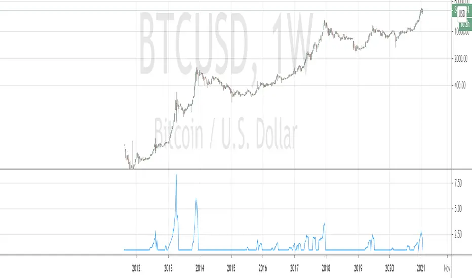
Bitcoin Buy Signal D/WThis is a Bitcoin buy-signal indicator, very simple to use:
It only works on daily and weekly timeframes.
When the Tulu line is above the Hani line, and the price moves back into the Tulu–Hani range, it’s a good buying opportunity.
When the Tulu line is below the Hani line, it’s better to wait for the price to return to Tromsø before buying.
Whenever the price is below Tromsø , it’s always a good time to buy.
Candles that meet these conditions are highlighted in bright yellow to make them easy to spot.
To the moon! 🚀
在腳本中搜尋"bitcoin"

Bitcoin Power Law Deviation Z-ScoreIntroduction While standard price charts show Bitcoin's exponential growth, it can be difficult to gauge exactly how "overheated" or "cheap" the asset is relative to its historical trend.
This indicator strips away the price action to visualize pure Deviation. It compares the current price to the Bitcoin Power Law "Fair Value" model and plots the result as a normalized Z-Score. This creates a clean oscillator that makes it easy to identify historical cycle tops and bottoms without the noise of a log-scale chart.
How to Read This Indicator The oscillator centers around a zero-line, which represents the mathematical "Fair Value" of the network. 0.0 (Center Line): Price is exactly at the Power Law fair value. Positive Values (+1 to +5): Price is trading at a premium. Historically, values above 4.0 have coincided with cycle peaks (Red Zones). Negative Values (-1 to -3): Price is trading at a discount. Historically, values below -1.0 have been excellent accumulation zones (Green/Blue Zones).
The Math Behind the Model This script uses the same physics-based Power Law parameters as the popular overlay charts: Formula: Price = A * (days since genesis)^b Slope (b): 5.78 Amplitude (A): 1.45 x 10^-17 The "Z-Score" is calculated by taking the logarithmic difference between the actual price and the model price, divided by a standard scaling factor (0.18 log steps).
How to Use Cycle Analysis: Use this tool to spot macro-extremes. Unlike RSI or MACD which reset frequently, this oscillator provides a multi-year view of market sentiment. Confluence: This tool works best when paired with the main "Power Law Rainbow" chart overlay to confirm whether price is hitting major resistance or support bands.
Credits Based on the Power Law theory by Giovanni Santostasi and Corridor concepts by Harold Christopher Burger .
Disclaimer This tool is for educational purposes only. Past performance of a model is not indicative of future results. Not financial advice.

Bitcoin Cycles Halvins/Tops/Bottoms By CrBeThis Script shows you the actual Bitcoin tops and bottoms dates.

Bitcoin Power Law Corridor + Z-score
This script visualizes the long-term Bitcoin Power Law Corridor, a conceptual model originally discussed by Harold Christopher Burger, and enhances it with a logarithmic Z-Score framework.
The indicator plots Bitcoin’s long-term regression curve together with estimated resistance and support bands based on power-law relationships between price and time since inception.
The added Z-Score expresses the statistical distance between price and the central regression line, using logarithmic scaling:
Z ≈ 0 → price near its long-term fair-value trajectory.
Z ≈ +2 → price near the lower corridor boundary (historically undervalued region).
Z ≈ −2 → price near the upper corridor boundary (historically overheated region).
This indicator is designed for visual and educational purposes only.
It should not be considered financial advice, a predictive model, or a signal provider.
Users should always combine this tool with other forms of technical, fundamental, and sentiment analysis to confirm confluence before making any decision.

Bitcoin Lagging (N Days)This indicator overlays Bitcoin’s price on any chart with a user-defined N-day lag. You can select the BTC symbol and timeframe (daily recommended), choose which price source to use (open, high, low, close, hlc3, ohlc4), and shift the series by a chosen number of days. An option to normalize the series to 100 at the first visible value is also available, along with the ability to display the original BTC line for comparison.
It is designed for traders and researchers who want to test lagging relationships between Bitcoin and other assets, observe correlation changes, or visualize how BTC’s past prices might align with current market movements. The lagging is calculated based on daily candles, so even if applied on intraday charts, the shift remains in daily units.
이 지표는 비트코인 가격을 원하는 차트 위에 N일 지연된 상태로 표시해 줍니다. 심볼과 타임프레임(일봉 권장)을 선택할 수 있으며, 가격 소스(시가, 고가, 저가, 종가, hlc3, ohlc4)도 설정 가능합니다. 또한 시리즈를 첫 값 기준으로 100에 맞춰 정규화하거나, 원래의 비트코인 가격선을 함께 표시할 수도 있습니다.
비트코인과 다른 자산 간의 시차 효과를 분석하거나 상관관계 변화를 관찰할 때 유용하게 활용할 수 있습니다. 지연은 일봉 기준으로 계산되므로, 분·시간 차트에 적용해도 항상 일 단위로 반영됩니다.
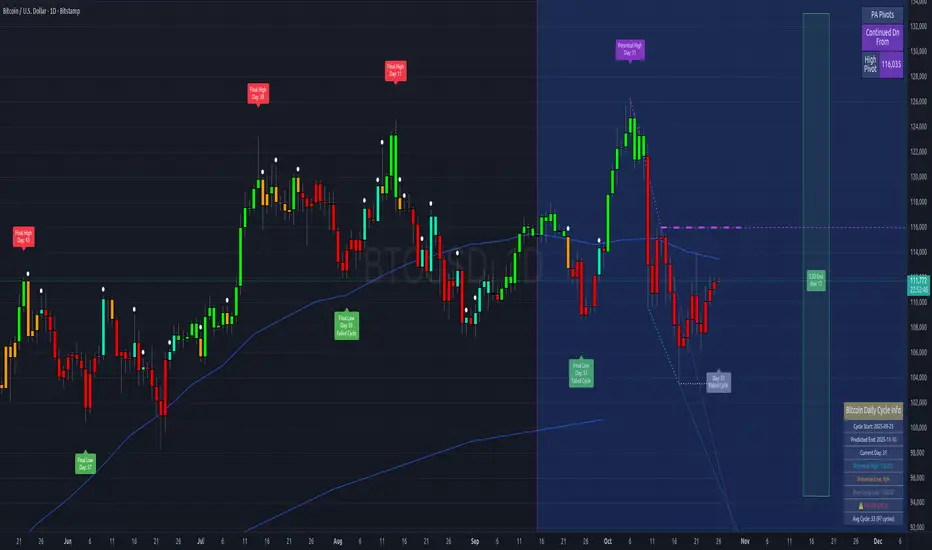
Bitcoin Cycles IndicatorTrack Bitcoin's cyclical price patterns across multiple timeframes with this cycle analysis tool. The indicator automatically identifies cycle lows and highs, marking them with clear visual labels that show cycle day counts and failed cycle detection.
Key Features:
Multi-Time frame Support - Optimized settings for Daily, Weekly, Monthly, and Custom time frames
Cycle Tracking - Identifies and labels cycle lows (green) and highs (red) with day counts
Failed Cycle Detection - Highlights when cycles break below previous lows
Customizable Settings - Adjust cycle lengths, colors, and display options for each timeframe
Info Box - Real-time cycle information display with current cycle day count
Projection Boxes - Visual cycle length projections for better analysis
Perfect for Bitcoin traders and analysts who want to understand market cycles and timing. Works best on Daily charts for short-term cycles and Weekly/Monthly charts for longer-term analysis.
Bitcoin Weekend FadeThis indicator is a tool for setting a bias based on weekend price movements, with the assumption that the crypto market often experiences stronger moves over the weekend due to thinner order books. It helps identify potential fade opportunities, suggesting that price movements from Saturday and Sunday may reverse during the weekdays.
How to use:
Sets a bias based on weekend price action.
Sets a bias based on weekend price action.
Use weekday price action for confirmation before acting on the bias.
Best suited for range-bound markets, where the price tends to revert to the mean.
Avoid fading high-timeframe breakouts, as they often indicate strong trends.

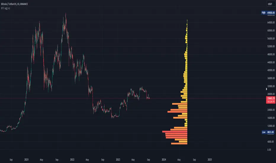
Bitcoin Aggregated Volume Profile «NoaTrader»If you use volume profile for analyzing Bitcoin, you may know that sometimes the decisions of big CEXs like Binance can change the volume of each symbol and so the analysis perceived from the data (which may not be valid anymore); Like when Binance decided to transfer the free transaction fee promotion from BTCUSDT to BTCTUSD pair or the new introduced BTCFDUSD pair with volume market share as much as BTCTUSD after only 1 month (according to the coinmarketcap's data).
This indicator tries to solve that problem for using volume profile. So, it collects all the volumes of different pairs from different exchanges and then uses all of them to calculate the volume profile.
Also, there is an option to compare the current symbols volume to the whole volume profile which is a Boolean option in the settings (the picture above)
The aggregated volume data includes:
BINANCE:BTCUSDT
BINANCE:BTCTUSD
BINANCE:BTCBUSD
BINANCE:BTCFDUSD
BINANCE:BTCDAI
BINANCE:BTCEUR
BITSTAMP:BTCUSDT
BITSTAMP:BTCUSD
COINBASE:BTCUSDT
COINBASE:BTCUSD
COINBASE:BTCEUR
HUOBI:BTCUSDT
KUCOIN:BTCUSDT
KRAKEN:XBTUSD
KRAKEN:XBTEUR
BITFINEX:BTCUSD
BYBIT:BTCUSDT
KRAKEN:BTCUSD
OKX:BTCUSDT
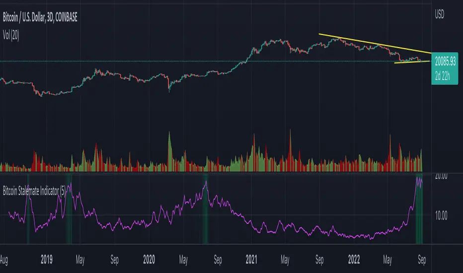
Bitcoin Stalemate IndicatorThe Bitcoin Stalemate Indicator examines periods in the market defined by a combination of high volume and low price volatility. These periods are a bit like a tug-of-war with both sides applying a lot of force but the rope moving very little. Periods of high volume and low volatility suggest both sides of the trade are stuck in a stalemate. This indicator may be useful in identifying psychologically important price levels.
The mechanics of the indicator are fairly simple: the indicator takes the volume and divides it by the candle’s size over it’s close for that same period.
volume / ((high - low) / close)
Candles that move very little but with high volume will produce higher reads and vice versa. Finally a smoothing average is applied to clean up the noise.
Volume profiles from the top 6 exchanges are averaged in order to avoid a single exchange’s popularity acting as an overriding factor. Single exchanges can be isolated but are of lesser use. Heat map functionality is only active when all exchanges are selected.
Bitcoin Scalping Strategy (Sampled with: PMARP+MADRID MA RIBBON)
DISCLAIMER:
THE CONTENT WITHIN THIS STRATEGY IS CREATED FROM TWO INDICATORS CREATED BY TWO PINESCRIPTER'S. THE STRATEGY WAS EXECUTED BY MYSELF AND REVERSE-ENGINEERED TO MEET THE CONDITIONS OF THE INTENDED STRATEGY REQUESTOR. I DO NOT TAKE CREDIT FOR THE CONTENT WITHIN THE ESTABLISHED LINES MADE CLEAR BY MYSELF.
The Sampled Scripts and creators:
PMAR/PMARP by @The_Caretaker Link to original script:
Madrid MA RIBBON BAR by @Madrid Link to original script:
Cheat Code's strategy notes:
This sampled strategy (Requested by @elemy_eth) is one combining previously created studies. I reverse-engineered the local scope for the Madrid moving average color plots and set entry and exit conditions for certain criteria met. This strategy is meant to deliver an extremely high hit rate on a daily time frame. This is made possible because of the very low take profit percentage, during the context of a macro downtrend it is made easier to hit 1-3% scalps which is made visible with the strategy using sampled scripts I created here.
How it works:
Entry Conditions:
-Enter Long's if the lime color conditions are met true using the script detailed by Marid's MA
- No re-entry into positions needs to be met true (this prevents pyramiding of orders due to conditions being met true) applicable to both long and short side entries.
- To increase hit rate and prevent traps both the parameters of rsi being sub 80 and no previously engulfing candles need to be met true to enter a long position.
- Enter Short's if the red color conditions of Madrid's moving average are met true.
- Closing Long positions are typically not met within this indicator, however, it still sometimes triggers if necessary. This consists of a pmarp sub 99 and a position size greater than 0.0
- Closing Short positions are typically not met within this indicator, however, it still sometimes triggers if necessary. This consists of a pmarp over 01 and a position size less than 0.0
- Stop Loss: 27.75% Take Profit: 1% (Which does not trigger on ticks over 1% so you will see average trade profits greater than 1%)
BYBIT:BTCUSDT BINANCE:BTCUSDT COINBASE:BTCUSD
Best Of Luck :)
-CheatCode1

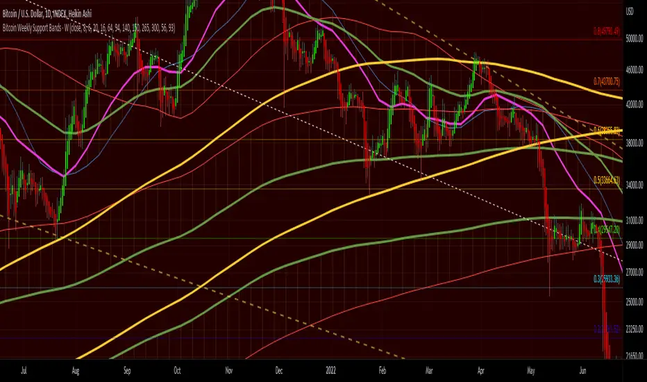
Bitcoin Weekly Support BandsMy first ever attempt at a custom script. I took Benjamin Cowen's concept of the Bitcoin Bull Market Support Band and applied it to the 100 week and 200 week moving averages. I also added in the 300 week sma. I mainly wanted to have all these in one indicator.
Bitcoin Bottom Detector: W TimeframeUse this indicator in the weekly time frame:
One of the most widely used indicators for identifying the Bitcoin market bottom is the 200-week moving average. This indicator works based on the ratio of price to the value of the 200-week moving average. When the indicator enters the lower blue part (overflow area), it indicates the bitcoin is in the bottom of the market.

Bitcoin Price Temperature: Weekly TimeframeUse this oscillator at weekly timeframes:
The Bitcoin Price Temperature (BPT) is an oscillator that models the number of standard deviations the price has moved away from the 4-yr moving average. This seeks to establish a mean reversion model based on the cyclical nature of Bitcoin halving and investment cycles. The BPT bands then establish price levels that coincide with specific standard deviation multiples to identify fair and extreme valuations.
Coined By:
DilutionProof
Interpretation:
Values above 6 indicate extremely high price areas: (TOP OF THE MARKET)
Areas below 0.2 indicate extremely low price areas: (BOTTOM OF THE MARKET)

Bitcoin trend RVI and Emastrategy with two emas and rvi.
Only long positions when fast ema above slow ema when rvi gives entry.
Only short positions when slow ema above fast ema when rvi gives entry.

Bitcoin Spot PremiumPlots the difference between the Bitcoin Spot price and the average of 7 Futures prices.
The idea being that Spot leads the market, and when Spot is priced significantly higher than Futures, price should increase. And vice-versa.
Possible uses:
Sharp changes could indicate a reversal is coming
A consistently large premium can be used as additional validation of trend continuation
Divergences may help identify trend exhaustion
If you find a strategy that works well with this indicator, I'd love to know. Enjoy!

Bitcoin Golden Bottom Oscillator (MZ BTC Oscillator)This indicator uses Elliot Wave Oscillator Methodology applied on "BTC Golden Bottom with Adaptive Moving Average" and Relative Strength Index of Resulted EVO to form an Oscillator to detect trend health in Bitcoin price. Ticker is set to "INDEX : BTCUSD" on 1D timeframe.
Methodology
Oscillator uses Adaptive Moving Average with 1 year of length, Minor length of 50 and Major length of 100 to mark AMA as Golden Bottom.
Percentage Elliot Wave Oscillator is calculated between BTC price and AMA.
Relative Strength Index of EVO is calculated to detect trend strength and divergence detection.
Hull Moving Average of resulted RSI is used to smoothen the Oscillator.
Oscillator is hard coded to 'INDEX:BTCUSD' ticker on 1d so it can be used on any other chart and on any other timeframe.
Color Schemes
Bright Red background color indicates that price has left top Fib multiple ATR band and possibly go for top.
Light Red background color indicates that price has left 2nd top Fib multiple ATR band and possibly go for local top.
Lime background color indicates that price has entered lowest band indicating local bottom.
Bright Green background color indicates that price is approximately resting on Golden Bottom i.e. AMA.
Oscillator color is set to gradient for easy directional adaption.
BTC Golden Bottom with Adaptive Moving Average

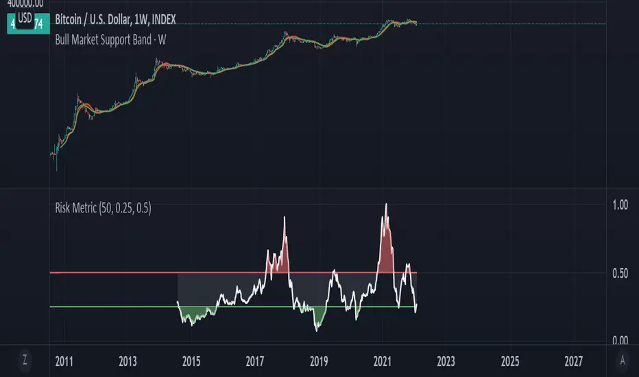
Bitcoin Risk Metric IIThesis: Bitcoin's price movements can be (dubiously) characterized by functional relationships between moving averages and standard deviations. These movements can be normalized into a risk metric through normalization functions of time. This risk metric may be able to quantify a long term "buy low, sell high" strategy.
This risk metric is the average of three normalized metrics:
1. (btc - 4 yma)/ (std dev)
2. ln(btc / 20 wma)
3. (50 dma)/(50 wma)
* btc = btc price
* yma = yearly moving average of btc, wma = weekly moving average of btc, dma = daily moving average of btc
* std dev = std dev of btc
Important note:
Historical data for this metric is only shown back until 2014, because of the nature of the 1st mentioned metric. The other two metrics produce a value back until 2011. A previous, less robust, version of metric 2 is posted on my TradingView as well.
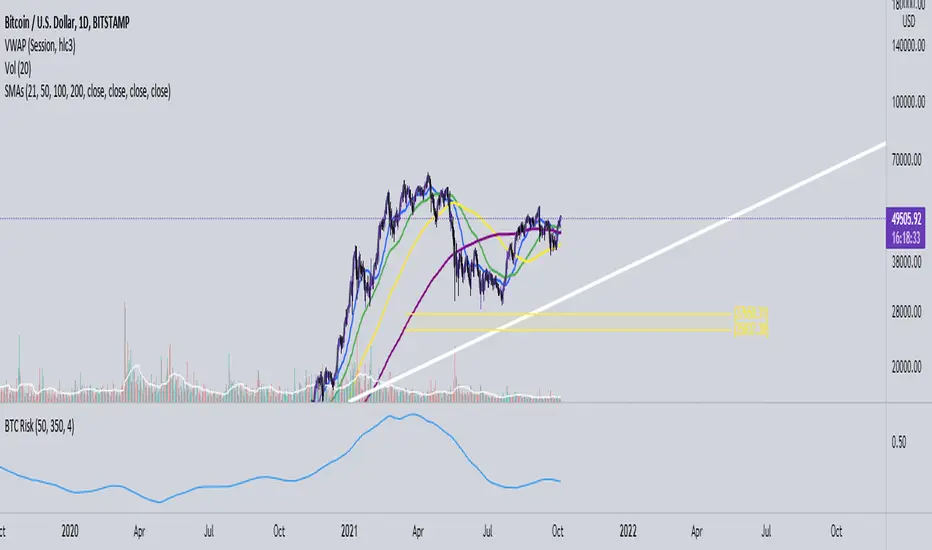
Bitcoin Risk Indicator (Daily)This indicator calculates the risk of buying and selling BTC, if the risk is reaching the upper boundaries of 0.8 to 1 then BTC is either getting close to a market cycle top or is far over extended.
If BTC is below 0.4 then this inidicates the least amount of Risk to buy BTC.
Bitcoin Halving EventsPast dates for the bitcoin halvings are marked with vertical yellow lines and labeled with the date and cycle number.

BTC COT Delta BBitcoin CME COT Delta Strategy
---------------------------------------
Reading 4 largest long positions and 4 largest short positions, this script uses (shorts - longs) to produce a long/short signal.
• When delta <= buy threshold, a "long" signal will appear on the chart.
• When shorts >= sell threshold, a "short" signal will appear on the chart.
To see the indicator below, since it's not possible to mix the two, use this script:
** This is not a trading advice, it's for research purposes only. Do not trade based upon these signals.

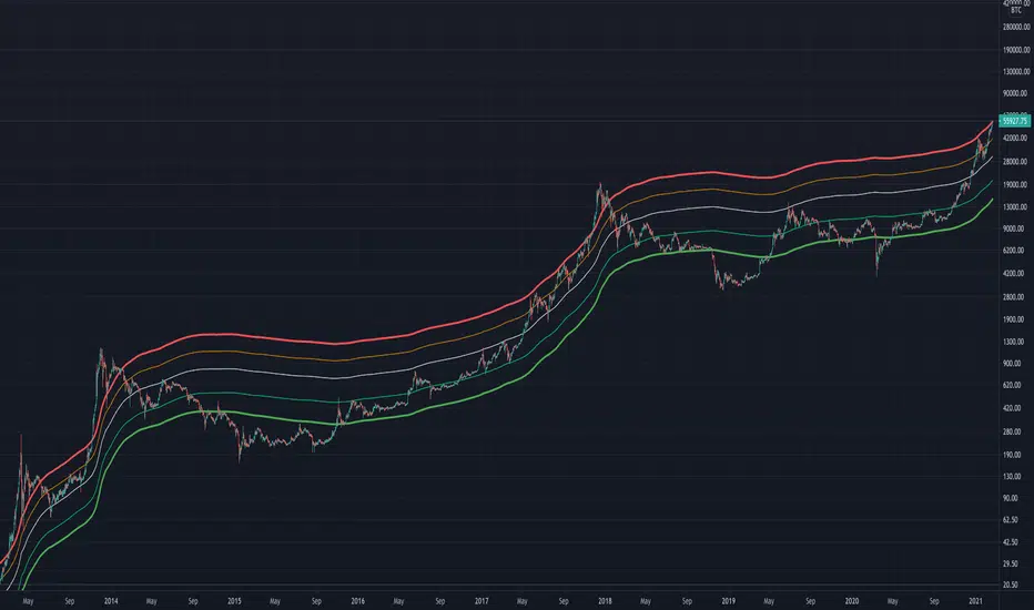
Bitcoin Investor ToolSimple and ugly long MA ribbon, Try at different intervals, but for me it's a good way to eyeball where we are currently in the bitcoin cycle.
Bitcoin Bubble Strength IndexFor those who interested, here is a Bitcoin Strength Index source code. I used it on weekly chart with params (close,28). And only with Bitcoin . And only during bull run. It shows how far price went off the particular moving average during bubble run (i.e. being above BB). Weekly MA 28 is approximately daily ma 200.
The physical meaning of this indicator is to show current bull rally "speed".