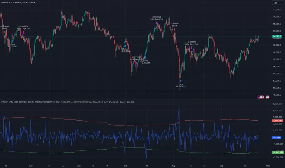
Bitcoin CME-Spot Z-Spread - Strategy [presentTrading]This time is a swing trading strategy! It measures the sentiment of the Bitcoin market through the spread of CME Bitcoin Futures and Bitfinex BTCUSD Spot prices. By applying Bollinger Bands to the spread, the strategy seeks to capture mean-reversion opportunities when prices deviate significantly from their historical norms
█ Introduction and How it is Different
The Bitcoin CME-Spot Bollinger Bands Strategy is designed to capture mean-reversion opportunities by exploiting the spread between CME Bitcoin Futures and Bitfinex BTCUSD Spot prices. The strategy uses Bollinger Bands to detect when the spread between these two correlated assets has deviated significantly from its historical norm, signaling potential overbought or oversold conditions.
What sets this strategy apart is its focus on spread trading between futures and spot markets rather than price-based indicators. By applying Bollinger Bands to the spread rather than individual prices, the strategy identifies price inefficiencies across markets, allowing traders to take advantage of the natural reversion to the mean that often occurs in these correlated assets.
BTCUSD 8hr Performance
█ Strategy, How It Works: Detailed Explanation
The strategy relies on Bollinger Bands to assess the volatility and relative deviation of the spread between CME Bitcoin Futures and Bitfinex BTCUSD Spot prices. Bollinger Bands consist of a moving average and two standard deviation bands, which help measure how much the spread deviates from its historical mean.
🔶 Spread Calculation:
The spread is calculated by subtracting the Bitfinex spot price from the CME Bitcoin futures price:
Spread = CME Price - Bitfinex Price
This spread represents the difference between the futures and spot markets, which may widen or narrow based on supply and demand dynamics in each market. By analyzing the spread, the strategy can detect when prices are too far apart (potentially overbought or oversold), indicating a trading opportunity.
🔶 Bollinger Bands Calculation:
The Bollinger Bands for the spread are calculated using a simple moving average (SMA) and the standard deviation of the spread over a defined period.
1. Moving Average (SMA):
The simple moving average of the spread (mu_S) over a specified period P is calculated as:
mu_S = (1/P) * sum(S_i from i=1 to P)
Where S_i represents the spread at time i, and P is the lookback period (default is 200 bars). The moving average provides a baseline for the normal spread behavior.
2. Standard Deviation:
The standard deviation (sigma_S) of the spread is calculated to measure the volatility of the spread:
sigma_S = sqrt((1/P) * sum((S_i - mu_S)^2 from i=1 to P))
3. Upper and Lower Bollinger Bands:
The upper and lower Bollinger Bands are derived by adding and subtracting a multiple of the standard deviation from the moving average. The number of standard deviations is determined by a user-defined parameter k (default is 2.618).
- Upper Band:
Upper Band = mu_S + (k * sigma_S)
- Lower Band:
Lower Band = mu_S - (k * sigma_S)
These bands provide a dynamic range within which the spread typically fluctuates. When the spread moves outside of these bands, it is considered overbought or oversold, potentially offering trading opportunities.
Local view
🔶 Entry Conditions:
- Long Entry: A long position is triggered when the spread crosses below the lower Bollinger Band, indicating that the spread has become oversold and is likely to revert upward.
Spread < Lower Band
- Short Entry: A short position is triggered when the spread crosses above the upper Bollinger Band, indicating that the spread has become overbought and is likely to revert downward.
Spread > Upper Band
🔶 Risk Management and Profit-Taking:
The strategy incorporates multi-step take profits to lock in gains as the trade moves in favor. The position is gradually reduced at predefined profit levels, reducing risk while allowing part of the trade to continue running if the price keeps moving favorably.
Additionally, the strategy uses a hold period exit mechanism. If the trade does not hit any of the take-profit levels within a certain number of bars, the position is closed automatically to avoid excessive exposure to market risks.
█ Trade Direction
The trade direction is based on deviations of the spread from its historical norm:
- Long Trade: The strategy enters a long position when the spread crosses below the lower Bollinger Band, signaling an oversold condition where the spread is expected to narrow.
- Short Trade: The strategy enters a short position when the spread crosses above the upper Bollinger Band, signaling an overbought condition where the spread is expected to widen.
These entries rely on the assumption of mean reversion, where extreme deviations from the average spread are likely to revert over time.
█ Usage
The Bitcoin CME-Spot Bollinger Bands Strategy is ideal for traders looking to capitalize on price inefficiencies between Bitcoin futures and spot markets. It’s especially useful in volatile markets where large deviations between futures and spot prices occur.
- Market Conditions: This strategy is most effective in correlated markets, like CME futures and spot Bitcoin. Traders can adjust the Bollinger Bands period and standard deviation multiplier to suit different volatility regimes.
- Backtesting: Before deployment, backtesting the strategy across different market conditions and timeframes is recommended to ensure robustness. Adjust the take-profit steps and hold periods to reflect the trader’s risk tolerance and market behavior.
█ Default Settings
The default settings provide a balanced approach to spread trading using Bollinger Bands but can be adjusted depending on market conditions or personal trading preferences.
🔶 Bollinger Bands Period (200 bars):
This defines the number of bars used to calculate the moving average and standard deviation for the Bollinger Bands. A longer period smooths out short-term fluctuations and focuses on larger, more significant trends. Adjusting the period affects the responsiveness of the strategy:
- Shorter periods (e.g., 100 bars): Makes the strategy more reactive to short-term market fluctuations, potentially generating more signals but increasing the risk of false positives.
- Longer periods (e.g., 300 bars): Focuses on longer-term trends, reducing the frequency of trades and focusing only on significant deviations.
🔶 Standard Deviation Multiplier (2.618):
The multiplier controls how wide the Bollinger Bands are around the moving average. By default, the bands are set at 2.618 standard deviations away from the average, ensuring that only significant deviations trigger trades.
- Higher multipliers (e.g., 3.0): Require a more extreme deviation to trigger trades, reducing trade frequency but potentially increasing the accuracy of signals.
- Lower multipliers (e.g., 2.0): Make the bands narrower, increasing the number of trade signals but potentially decreasing their reliability.
🔶 Take-Profit Levels:
The strategy has four take-profit levels to gradually lock in profits:
- Level 1 (3%): 25% of the position is closed at a 3% profit.
- Level 2 (8%): 20% of the position is closed at an 8% profit.
- Level 3 (14%): 15% of the position is closed at a 14% profit.
- Level 4 (21%): 10% of the position is closed at a 21% profit.
Adjusting these take-profit levels affects how quickly profits are realized:
- Lower take-profit levels: Capture gains more quickly, reducing risk but potentially cutting off larger profits.
- Higher take-profit levels: Let trades run longer, aiming for bigger gains but increasing the risk of price reversals before profits are locked in.
🔶 Hold Days (20 bars):
The strategy automatically closes the position after 20 bars if none of the take-profit levels are hit. This feature prevents trades from being held indefinitely, especially if market conditions are stagnant. Adjusting this:
- Shorter hold periods: Reduce the duration of exposure, minimizing risks from market changes but potentially closing trades too early.
- Longer hold periods: Allow trades to stay open longer, increasing the chance for mean reversion but also increasing exposure to unfavorable market conditions.
By understanding how these default settings affect the strategy’s performance, traders can optimize the Bitcoin CME-Spot Bollinger Bands Strategy to their preferences, adapting it to different market environments and risk tolerances.
在腳本中搜尋"bitcoin"
Bitcoin Fundamentals - Bitcoin Block RewardThe Bitcoin Block Reward is the batch of new Bitcoins generated by the miners after solving each block.
The Block Reward is set as a basic rule and cannot be changed without agreement between the entire Bitcoin network. It started at 50 BTC during the first period. Afterwards the Block Reward gets adjusted to half of it value (Halving Event) on each cycle of 210000 blocks mined.
This is the only way that new bitcoins are created. It creates an incentive for miners to secure the network.
Over time the Block Reward will decreases to a value that might not cover the mining costs. At that point, the use of the Bitcoin Network might have increased sufficiently as to generate enough transaction fees to cover the mining costs.
MOTIVATION
Even though this is a very simple indicator, I'm currently missing a data source to compute the Block Reward value within Tradingview. Therefore, I created this indicator and its associated library function to enable its visualization and (eventually) for coders to make use of the source function to power more elaborate scripts related to the Halving Events.
Hope that helps!

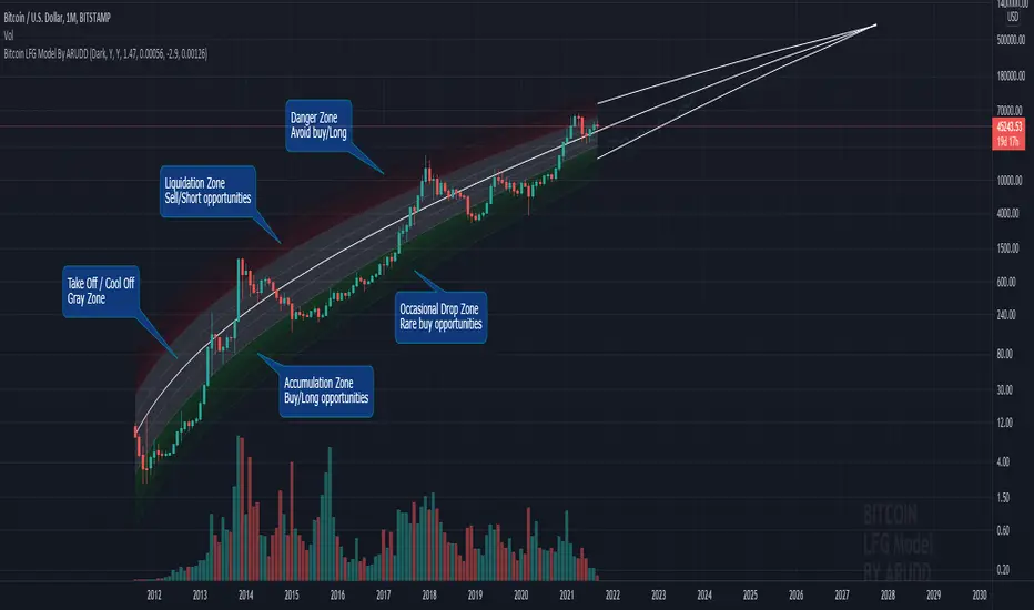
Bitcoin Logarithmic Fractal Growth Model By ARUDDThis model, which I'm calling the Logarithmic Fractal Growth Mode (L.F.G) , uses Bitcoin's mathematical monetary policy to evaluate the future possible price valuation.
It takes into account fractal (and logarithmic) growth as well as how those who hold bitcoins might react to certain events such as changes in supply and demand. It also shows that it is mathematically logical that someday it must become stable.
The information gained from knowing this helps people make more informed decisions when buying bitcoin and thinking of its future possibilities.
The model can serve as some type of general guideline for determining how much bitcoins should be worth in the future if it follows a certain path from its current price.
Modeling Bitcoin's money supply mathematically, and knowing that there is a finite number of them, makes this whole process much more rational than just thinking about the possibilities in pure subjective terms.
Before going any further I want to say that no one can know with absolute certainty what will happen to bitcoins price in the future, but using mathematics gives us an idea of where things are headed.
The results presented here are based on very reasonable assumptions for how bitcoin might continue to grow (and then level out) once there are over 21 million bitcoins in existence.
The model shows that bitcoin's price can never go down to zero (thus creating the "death spiral" phenomenon), and as such, bitcoin has an extremely high probability of becoming stable as it approaches infinity.
Conversely, this model also shows that at some point there is a high probability that bitcoin will not continue to grow exponentially forever.
Credit goes to Quantadelic for the awesome original script.
ARUDD
Bitcoin Comparison to GBTC!This script tells you if GBTC is overvalued or undervalued compared to Bitcoin.

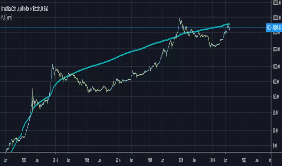
Bitcoin Price User Correlation [aamonkey]You can only use this for BTC.
Bitcoin over time tends to be priced at 7000 times the number of users (in terms of market cap).
Calculation:
Number of Wallets*7000/(Circulating Supply or 21,000,000)
Settings:
You can decide whether you want to use the Circulating Supply or 21,000,000 as a reference.
The default settings are using 21,000,000 because it seems to be more accurate.
You can easily switch between both versions by checking the box in the settings.
Interesting Findings:
Using circulating supply:
- Most of the time we are under the estimated ("PUC") line
- Once we break above the PUC line we are in the parabolic phase of the Bullrun
- In history, we broke only 4 times above the PUC
- Once we are above the PUC we see crazy growth (parabolic phase)
- We don't spend much time above the PUC
- From breaking the PUC to the new All-Time High of the cycle we took in order: 3 Days, 7 Days, 22 Days, 30 Days
- So the trend is increasing (We are taking more and more time until we see the ATH)
- Currently, we are about to break the PUC
- Then I expect the parabolic phase to begin
- I expect the run to last about 30 days
Bitcoin CME gaps multi-timeframe auto finder1. Overview
The Bitcoin CME Gap Multi-Timeframe Detector automatically identifies price gaps in the Bitcoin CME (Chicago Mercantile Exchange) futures market and visually displays them on the TradingView chart.
Because the CME futures market closes for about an hour after each weekday session and remains closed over the weekend, price gaps frequently appear when trading resumes on Monday.
This indicator analyzes gaps across six major timeframes, from 5-minute to 1-day charts, allowing traders to easily identify structural imbalances and potential support/resistance zones.
It is the most accurate and feature-rich CME gaps indicator available on TradingView.
2. Key Features
■ Multi-Timeframe Gap Detection
Analyzes 5m, 15m, 30m, 1h, 4h, and 1D charts simultaneously.
This enables traders to observe both short-term volatility and mid-to-long-term structure, providing a multi-dimensional view of market dynamics.
■ Gap Direction Classification
Up Gap: When the next candle’s open is higher than the previous candle’s high (default color: green tone)
Down Gap: When the next candle’s open is lower than the previous candle’s low (default color: red tone)
Gaps are color-coded to intuitively visualize potential support and resistance zones.
■ Highlight Function
Gaps exceeding a user-defined threshold (%) are highlighted (default color: yellow).
This helps quickly identify zones with abnormal volatility or sharp price dislocations.
■ Labels and Box Extension
Each gap displays a percentage label indicating its relative size and significance.
Gap zones are extended to the right as boxes, allowing traders to visually track when and how the gap gets filled over time.
■ Alert System
When a gap forms on the selected timeframe (or across all timeframes), a TradingView alert is triggered.
This enables real-time response to significant gap events.
3. Trading Strategies
■ Gap Fill Behavior
CME gaps statistically tend to get filled over time.
Gap boxes help distinguish between filled and unfilled gaps at a glance.
Up Gap: Price tends to decline to fill the previous high–next open zone.
Down Gap: Price often rises later to fill the previous low–next open zone.
■ Support & Resistance Levels
Gap zones frequently act as strong support or resistance.
When price retests a gap area, observing the reaction of buyers and sellers can provide valuable trading insights.
Overlapping gap boxes across multiple timeframes indicate high-confidence support/resistance zones.
■ Market Sentiment & Volatility Analysis
Large gaps usually result from shifts in market sentiment or major news events.
This indicator allows traders to detect volatility spikes early and prepare for potential trend reversals.
■ Combination with Other Technical Tools
While fully functional on its own, this indicator works even better when combined with tools like moving averages (MA), RSI, MACD, or Fibonacci retracements.
For example, if the bottom of a gap coincides with the 0.618 Fibonacci level, it may signal a strong rebound zone.
4. Settings Options
Minimum Gap % | Sets the minimum percentage movement required to detect a gap (lower values show smaller gaps)
Display Timeframes | Choose which timeframes to display (5m, 15m, 30m, 1h, 4h, 1D)
Box Colors | Assign colors for up and down gaps
Box Extension (Bars) | Number of bars to extend gap boxes to the right
Show Labels | Toggle display of gap percentage labels
Label Position / Size | Adjust label position and size
Highlight Gap ≥ % | Highlight gaps exceeding a specified percentage
Highlight Colors | Set highlight color for labels and boxes
Enable Alerts | Enable or disable alerts
Alert Timeframe | Select timeframe(s) for alerts (“All” = all timeframes)
5. Summary
This indicator is a professional trading tool that provides quantitative and visual analysis of price gaps in the Bitcoin CME futures market.
By combining multi-timeframe detection, highlighting, and alert systems, it helps traders clearly identify zones of market imbalance and potential reversal areas.

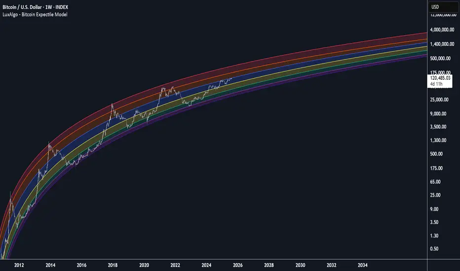
Bitcoin Expectile Model [LuxAlgo]The Bitcoin Expectile Model is a novel approach to forecasting Bitcoin, inspired by the popular Bitcoin Quantile Model by PlanC. By fitting multiple Expectile regressions to the price, we highlight zones of corrections or accumulations throughout the Bitcoin price evolution.
While we strongly recommend using this model with the Bitcoin All Time History Index INDEX:BTCUSD on the 3 days or weekly timeframe using a logarithmic scale, this model can be applied to any asset using the daily timeframe or superior.
Please note that here on TradingView, this model was solely designed to be used on the Bitcoin 1W chart, however, it can be experimented on other assets or timeframes if of interest.
🔶 USAGE
The Bitcoin Expectile Model can be applied similarly to models used for Bitcoin, highlighting lower areas of possible accumulation (support) and higher areas that allow for the anticipation of potential corrections (resistance).
By default, this model fits 7 individual Expectiles Log-Log Regressions to the price, each with their respective expectile ( tau ) values (here multiplied by 100 for the user's convenience). Higher tau values will return a fit closer to the higher highs made by the price of the asset, while lower ones will return fits closer to the lower prices observed over time.
Each zone is color-coded and has a specific interpretation. The green zone is a buy zone for long-term investing, purple is an anomaly zone for market bottoms that over-extend, while red is considered the distribution zone.
The fits can be extrapolated, helping to chart a course for the possible evolution of Bitcoin prices. Users can select the end of the forecast as a date using the "Forecast End" setting.
While the model is made for Bitcoin using a log scale, other assets showing a tendency to have a trend evolving in a single direction can be used. See the chart above on QQQ weekly using a linear scale as an example.
The Start Date can also allow fitting the model more locally, rather than over a large range of prices. This can be useful to identify potential shorter-term support/resistance areas.
🔶 DETAILS
🔹 On Quantile and Expectile Regressions
Quantile and Expectile regressions are similar; both return extremities that can be used to locate and predict prices where tops/bottoms could be more likely to occur.
The main difference lies in what we are trying to minimize, which, for Quantile regression, is commonly known as Quantile loss (or pinball loss), and for Expectile regression, simply Expectile loss.
You may refer to external material to go more in-depth about these loss functions; however, while they are similar and involve weighting specific prices more than others relative to our parameter tau, Quantile regression involves minimizing a weighted mean absolute error, while Expectile regression minimizes a weighted squared error.
The squared error here allows us to compute Expectile regression more easily compared to Quantile regression, using Iteratively reweighted least squares. For Quantile regression, a more elaborate method is needed.
In terms of comparison, Quantile regression is more robust, and easier to interpret, with quantiles being related to specific probabilities involving the underlying cumulative distribution function of the dataset; on the other expectiles are harder to interpret.
🔹 Trimming & Alterations
It is common to observe certain models ignoring very early Bitcoin price ranges. By default, we start our fit at the date 2010-07-16 to align with existing models.
By default, the model uses the number of time units (days, weeks...etc) elapsed since the beginning of history + 1 (to avoid NaN with log) as independent variable, however the Bitcoin All Time History Index INDEX:BTCUSD do not include the genesis block, as such users can correct for this by enabling the "Correct for Genesis block" setting, which will add the amount of missed bars from the Genesis block to the start oh the chart history.
🔶 SETTINGS
Start Date: Starting interval of the dataset used for the fit.
Correct for genesis block: When enabled, offset the X axis by the number of bars between the Bitcoin genesis block time and the chart starting time.
🔹 Expectiles
Toggle: Enable fit for the specified expectile. Disabling one fit will make the script faster to compute.
Expectile: Expectile (tau) value multiplied by 100 used for the fit. Higher values will produce fits that are located near price tops.
🔹 Forecast
Forecast End: Time at which the forecast stops.
🔹 Model Fit
Iterations Number: Number of iterations performed during the reweighted least squares process, with lower values leading to less accurate fits, while higher values will take more time to compute.
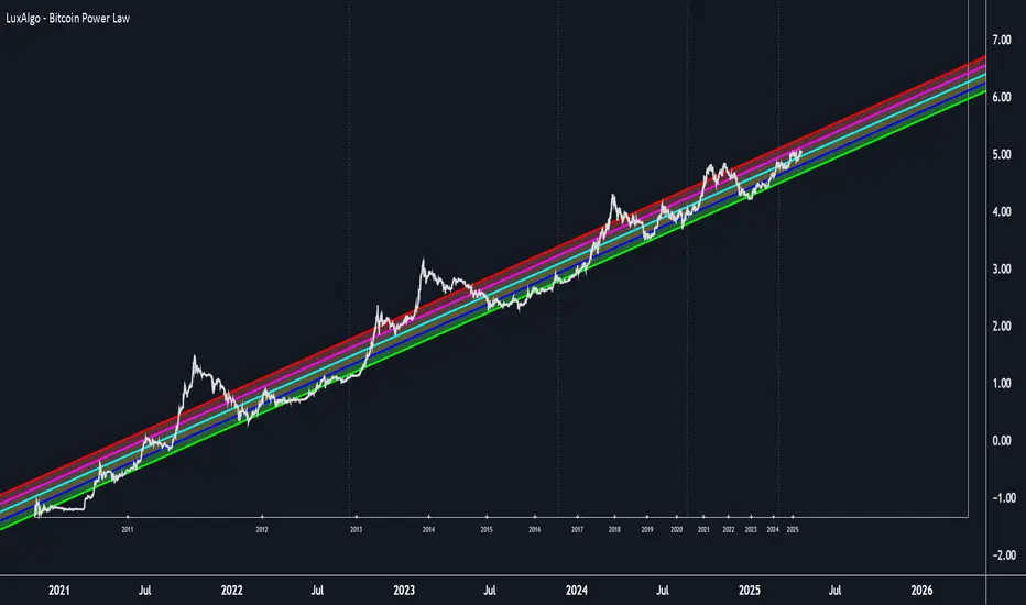
Bitcoin Power Law [LuxAlgo]The Bitcoin Power Law tool is a representation of Bitcoin prices first proposed by Giovanni Santostasi, Ph.D. It plots BTCUSD daily closes on a log10-log10 scale, and fits a linear regression channel to the data.
This channel helps traders visualise when the price is historically in a zone prone to tops or located within a discounted zone subject to future growth.
🔶 USAGE
Giovanni Santostasi, Ph.D. originated the Bitcoin Power-Law Theory; this implementation places it directly on a TradingView chart. The white line shows the daily closing price, while the cyan line is the best-fit regression.
A channel is constructed from the linear fit root mean squared error (RMSE), we can observe how price has repeatedly oscillated between each channel areas through every bull-bear cycle.
Excursions into the upper channel area can be followed by price surges and finishing on a top, whereas price touching the lower channel area coincides with a cycle low.
Users can change the channel areas multipliers, helping capture moves more precisely depending on the intended usage.
This tool only works on the daily BTCUSD chart. Ticker and timeframe must match exactly for the calculations to remain valid.
🔹 Linear Scale
Users can toggle on a linear scale for the time axis, in order to obtain a higher resolution of the price, (this will affect the linear regression channel fit, making it look poorer).
🔶 DETAILS
One of the advantages of the Power Law Theory proposed by Giovanni Santostasi is its ability to explain multiple behaviors of Bitcoin. We describe some key points below.
🔹 Power-Law Overview
A power law has the form y = A·xⁿ , and Bitcoin’s key variables follow this pattern across many orders of magnitude. Empirically, price rises roughly with t⁶, hash-rate with t¹² and the number of active addresses with t³.
When we plot these on log-log axes they appear as straight lines, revealing a scale-invariant system whose behaviour repeats proportionally as it grows.
🔹 Feedback-Loop Dynamics
Growth begins with new users, whose presence pushes the price higher via a Metcalfe-style square-law. A richer price pool funds more mining hardware; the Difficulty Adjustment immediately raises the hash-rate requirement, keeping profit margins razor-thin.
A higher hash rate secures the network, which in turn attracts the next wave of users. Because risk and Difficulty act as braking forces, user adoption advances as a power of three in time rather than an unchecked S-curve. This circular causality repeats without end, producing the familiar boom-and-bust cadence around the long-term power-law channel.
🔹 Scale Invariance & Predictions
Scale invariance means that enlarging the timeline in log-log space leaves the trajectory unchanged.
The same geometric proportions that described the first dollar of value can therefore extend to a projected million-dollar bitcoin, provided no catastrophic break occurs. Institutional ETF inflows supply fresh capital but do not bend the underlying slope; only a persistent deviation from the line would falsify the current model.
🔹 Implications
The theory assigns scarcity no direct role; iterative feedback and the Difficulty Adjustment are sufficient to govern Bitcoin’s expansion. Long-term valuation should focus on position within the power-law channel, while bubbles—sharp departures above trend that later revert—are expected punctuations of an otherwise steady climb.
Beyond about 2040, disruptive technological shifts could alter the parameters, but for the next order of magnitude the present slope remains the simplest, most robust guide.
Bitcoin behaves less like a traditional asset and more like a self-organising digital organism whose value, security, and adoption co-evolve according to immutable power-law rules.
🔶 SETTINGS
🔹 General
Start Calculation: Determine the start date used by the calculation, with any prior prices being ignored. (default - 15 Jul 2010)
Use Linear Scale for X-Axis: Convert the horizontal axis from log(time) to linear calendar time
🔹 Linear Regression
Show Regression Line: Enable/disable the central power-law trend line
Regression Line Color: Choose the colour of the regression line
Mult 1: Toggle line & fill, set multiplier (default +1), pick line colour and area fill colour
Mult 2: Toggle line & fill, set multiplier (default +0.5), pick line colour and area fill colour
Mult 3: Toggle line & fill, set multiplier (default -0.5), pick line colour and area fill colour
Mult 4: Toggle line & fill, set multiplier (default -1), pick line colour and area fill colour
🔹 Style
Price Line Color: Select the colour of the BTC price plot
Auto Color: Automatically choose the best contrast colour for the price line
Price Line Width: Set the thickness of the price line (1 – 5 px)
Show Halvings: Enable/disable dotted vertical lines at each Bitcoin halving
Halvings Color: Choose the colour of the halving lines
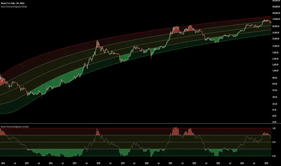
Bitcoin Polynomial Regression ModelThis is the main version of the script. Click here for the Oscillator part of the script.
💡Why this model was created:
One of the key issues with most existing models, including our own Bitcoin Log Growth Curve Model , is that they often fail to realistically account for diminishing returns. As a result, they may present overly optimistic bull cycle targets (hence, we introduced alternative settings in our previous Bitcoin Log Growth Curve Model).
This new model however, has been built from the ground up with a primary focus on incorporating the principle of diminishing returns. It directly responds to this concept, which has been briefly explored here .
📉The theory of diminishing returns:
This theory suggests that as each four-year market cycle unfolds, volatility gradually decreases, leading to more tempered price movements. It also implies that the price increase from one cycle peak to the next will decrease over time as the asset matures. The same pattern applies to cycle lows and the relationship between tops and bottoms. In essence, these price movements are interconnected and should generally follow a consistent pattern. We believe this model provides a more realistic outlook on bull and bear market cycles.
To better understand this theory, the relationships between cycle tops and bottoms are outlined below:https://www.tradingview.com/x/7Hldzsf2/
🔧Creation of the model:
For those interested in how this model was created, the process is explained here. Otherwise, feel free to skip this section.
This model is based on two separate cubic polynomial regression lines. One for the top price trend and another for the bottom. Both follow the general cubic polynomial function:
ax^3 +bx^2 + cx + d.
In this equation, x represents the weekly bar index minus an offset, while a, b, c, and d are determined through polynomial regression analysis. The input (x, y) values used for the polynomial regression analysis are as follows:
Top regression line (x, y) values:
113, 18.6
240, 1004
451, 19128
655, 65502
Bottom regression line (x, y) values:
103, 2.5
267, 211
471, 3193
676, 16255
The values above correspond to historical Bitcoin cycle tops and bottoms, where x is the weekly bar index and y is the weekly closing price of Bitcoin. The best fit is determined using metrics such as R-squared values, residual error analysis, and visual inspection. While the exact details of this evaluation are beyond the scope of this post, the following optimal parameters were found:
Top regression line parameter values:
a: 0.000202798
b: 0.0872922
c: -30.88805
d: 1827.14113
Bottom regression line parameter values:
a: 0.000138314
b: -0.0768236
c: 13.90555
d: -765.8892
📊Polynomial Regression Oscillator:
This publication also includes the oscillator version of the this model which is displayed at the bottom of the screen. The oscillator applies a logarithmic transformation to the price and the regression lines using the formula log10(x) .
The log-transformed price is then normalized using min-max normalization relative to the log-transformed top and bottom regression line with the formula:
normalized price = log(close) - log(bottom regression line) / log(top regression line) - log(bottom regression line)
This transformation results in a price value between 0 and 1 between both the regression lines. The Oscillator version can be found here.
🔍Interpretation of the Model:
In general, the red area represents a caution zone, as historically, the price has often been near its cycle market top within this range. On the other hand, the green area is considered an area of opportunity, as historically, it has corresponded to the market bottom.
The top regression line serves as a signal for the absolute market cycle peak, while the bottom regression line indicates the absolute market cycle bottom.
Additionally, this model provides a predicted range for Bitcoin's future price movements, which can be used to make extrapolated predictions. We will explore this further below.
🔮Future Predictions:
Finally, let's discuss what this model actually predicts for the potential upcoming market cycle top and the corresponding market cycle bottom. In our previous post here , a cycle interval analysis was performed to predict a likely time window for the next cycle top and bottom:
In the image, it is predicted that the next top-to-top cycle interval will be 208 weeks, which translates to November 3rd, 2025. It is also predicted that the bottom-to-top cycle interval will be 152 weeks, which corresponds to October 13th, 2025. On the macro level, these two dates align quite well. For our prediction, we take the average of these two dates: October 24th 2025. This will be our target date for the bull cycle top.
Now, let's do the same for the upcoming cycle bottom. The bottom-to-bottom cycle interval is predicted to be 205 weeks, which translates to October 19th, 2026, and the top-to-bottom cycle interval is predicted to be 259 weeks, which corresponds to October 26th, 2026. We then take the average of these two dates, predicting a bear cycle bottom date target of October 19th, 2026.
Now that we have our predicted top and bottom cycle date targets, we can simply reference these two dates to our model, giving us the Bitcoin top price prediction in the range of 152,000 in Q4 2025 and a subsequent bottom price prediction in the range of 46,500 in Q4 2026.
For those interested in understanding what this specifically means for the predicted diminishing return top and bottom cycle values, the image below displays these predicted values. The new values are highlighted in yellow:
And of course, keep in mind that these targets are just rough estimates. While we've done our best to estimate these targets through a data-driven approach, markets will always remain unpredictable in nature. What are your targets? Feel free to share them in the comment section below.

Bitcoin Polynomial Regression OscillatorThis is the oscillator version of the script. Click here for the other part of the script.
💡Why this model was created:
One of the key issues with most existing models, including our own Bitcoin Log Growth Curve Model , is that they often fail to realistically account for diminishing returns. As a result, they may present overly optimistic bull cycle targets (hence, we introduced alternative settings in our previous Bitcoin Log Growth Curve Model).
This new model however, has been built from the ground up with a primary focus on incorporating the principle of diminishing returns. It directly responds to this concept, which has been briefly explored here .
📉The theory of diminishing returns:
This theory suggests that as each four-year market cycle unfolds, volatility gradually decreases, leading to more tempered price movements. It also implies that the price increase from one cycle peak to the next will decrease over time as the asset matures. The same pattern applies to cycle lows and the relationship between tops and bottoms. In essence, these price movements are interconnected and should generally follow a consistent pattern. We believe this model provides a more realistic outlook on bull and bear market cycles.
To better understand this theory, the relationships between cycle tops and bottoms are outlined below:https://www.tradingview.com/x/7Hldzsf2/
🔧Creation of the model:
For those interested in how this model was created, the process is explained here. Otherwise, feel free to skip this section.
This model is based on two separate cubic polynomial regression lines. One for the top price trend and another for the bottom. Both follow the general cubic polynomial function:
ax^3 +bx^2 + cx + d.
In this equation, x represents the weekly bar index minus an offset, while a, b, c, and d are determined through polynomial regression analysis. The input (x, y) values used for the polynomial regression analysis are as follows:
Top regression line (x, y) values:
113, 18.6
240, 1004
451, 19128
655, 65502
Bottom regression line (x, y) values:
103, 2.5
267, 211
471, 3193
676, 16255
The values above correspond to historical Bitcoin cycle tops and bottoms, where x is the weekly bar index and y is the weekly closing price of Bitcoin. The best fit is determined using metrics such as R-squared values, residual error analysis, and visual inspection. While the exact details of this evaluation are beyond the scope of this post, the following optimal parameters were found:
Top regression line parameter values:
a: 0.000202798
b: 0.0872922
c: -30.88805
d: 1827.14113
Bottom regression line parameter values:
a: 0.000138314
b: -0.0768236
c: 13.90555
d: -765.8892
📊Polynomial Regression Oscillator:
This publication also includes the oscillator version of the this model which is displayed at the bottom of the screen. The oscillator applies a logarithmic transformation to the price and the regression lines using the formula log10(x) .
The log-transformed price is then normalized using min-max normalization relative to the log-transformed top and bottom regression line with the formula:
normalized price = log(close) - log(bottom regression line) / log(top regression line) - log(bottom regression line)
This transformation results in a price value between 0 and 1 between both the regression lines.
🔍Interpretation of the Model:
In general, the red area represents a caution zone, as historically, the price has often been near its cycle market top within this range. On the other hand, the green area is considered an area of opportunity, as historically, it has corresponded to the market bottom.
The top regression line serves as a signal for the absolute market cycle peak, while the bottom regression line indicates the absolute market cycle bottom.
Additionally, this model provides a predicted range for Bitcoin's future price movements, which can be used to make extrapolated predictions. We will explore this further below.
🔮Future Predictions:
Finally, let's discuss what this model actually predicts for the potential upcoming market cycle top and the corresponding market cycle bottom. In our previous post here , a cycle interval analysis was performed to predict a likely time window for the next cycle top and bottom:
In the image, it is predicted that the next top-to-top cycle interval will be 208 weeks, which translates to November 3rd, 2025. It is also predicted that the bottom-to-top cycle interval will be 152 weeks, which corresponds to October 13th, 2025. On the macro level, these two dates align quite well. For our prediction, we take the average of these two dates: October 24th 2025. This will be our target date for the bull cycle top.
Now, let's do the same for the upcoming cycle bottom. The bottom-to-bottom cycle interval is predicted to be 205 weeks, which translates to October 19th, 2026, and the top-to-bottom cycle interval is predicted to be 259 weeks, which corresponds to October 26th, 2026. We then take the average of these two dates, predicting a bear cycle bottom date target of October 19th, 2026.
Now that we have our predicted top and bottom cycle date targets, we can simply reference these two dates to our model, giving us the Bitcoin top price prediction in the range of 152,000 in Q4 2025 and a subsequent bottom price prediction in the range of 46,500 in Q4 2026.
For those interested in understanding what this specifically means for the predicted diminishing return top and bottom cycle values, the image below displays these predicted values. The new values are highlighted in yellow:
And of course, keep in mind that these targets are just rough estimates. While we've done our best to estimate these targets through a data-driven approach, markets will always remain unpredictable in nature. What are your targets? Feel free to share them in the comment section below.
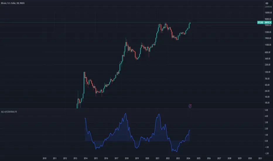
Bitcoin Bubble Risk (Adjusted for Diminishing Returns)Description:
This indicator offers a unique lens through which traders can assess risk in the Bitcoin market, specifically tailored to recognize the phenomenon of diminishing returns. By calculating the natural logarithm of the price relative to a 20-month Simple Moving Average (SMA) and applying a dynamic normalization process, this tool highlights periods of varying risk based on historical price movements and adjusted returns. The indicator is designed to provide nuanced insights into potential risk levels, aiding traders in their decision-making processes.
Usage:
To effectively use this indicator, apply it to your chart while ensuring that Bitcoin's price is set to display in monthly candles. This setting is vital for the indicator to accurately reflect the market's risk levels, as it relies on long-term data aggregation to inform its analysis.
This tool is especially beneficial for traders focused on medium to long-term investment horizons in Bitcoin, offering insights into when the market may be entering higher or lower risk phases. By incorporating this indicator into your analysis, you can gain a deeper understanding of potential risk exposures based on the adjusted price trends and market conditions.
Originality and Utility:
This script stands out for its innovative approach to risk analysis in the cryptocurrency space. By adjusting for the diminishing returns seen in mature markets, it provides a refined perspective on risk levels, enhancing traditional methodologies. This script is a significant contribution to the TradingView community, offering a unique tool for traders aiming to navigate the complexities of the Bitcoin market with informed risk management strategies.
Important Note:
This indicator is for informational purposes only and should not be considered investment advice. Users are encouraged to conduct their own research and consult with financial professionals before making investment decisions. The accuracy of the indicator's predictions can only be ensured when applied to monthly candlestick charts of Bitcoin.
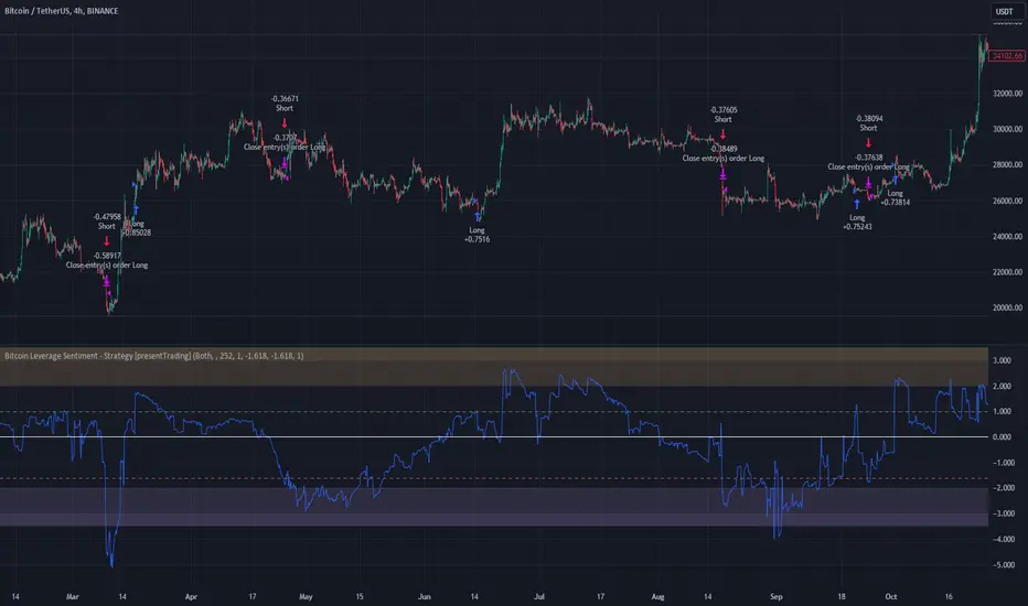
Bitcoin Leverage Sentiment - Strategy [presentTrading]█ Introduction and How it is Different
The "Bitcoin Leverage Sentiment - Strategy " represents a novel approach in the realm of cryptocurrency trading by focusing on sentiment analysis through leveraged positions in Bitcoin. Unlike traditional strategies that primarily rely on price action or technical indicators, this strategy leverages the power of Z-Score analysis to gauge market sentiment by examining the ratio of leveraged long to short positions. By assessing how far the current sentiment deviates from the historical norm, it provides a unique lens to spot potential reversals or continuation in market trends, making it an innovative tool for traders who wish to incorporate market psychology into their trading arsenal.
BTC 4h L/S Performance
local
█ Strategy, How It Works: Detailed Explanation
🔶 Data Collection and Ratio Calculation
Firstly, the strategy acquires data on leveraged long (**`priceLongs`**) and short positions (**`priceShorts`**) for Bitcoin. The primary metric of interest is the ratio of long positions relative to the total of both long and short positions:
BTC Ratio=priceLongs / (priceLongs+priceShorts)
This ratio reflects the prevailing market sentiment, where values closer to 1 indicate a bullish sentiment (dominance of long positions), and values closer to 0 suggest bearish sentiment (prevalence of short positions).
🔶 Z-Score Calculation
The Z-Score is then calculated to standardize the BTC Ratio, allowing for comparison across different time periods. The Z-Score formula is:
Z = (X - μ) / σ
Where:
- X is the current BTC Ratio.
- μ is the mean of the BTC Ratio over a specified period (**`zScoreCalculationPeriod`**).
- σ is the standard deviation of the BTC Ratio over the same period.
The Z-Score helps quantify how far the current sentiment deviates from the historical norm, with high positive values indicating extreme bullish sentiment and high negative values signaling extreme bearish sentiment.
🔶 Signal Generation: Trading signals are derived from the Z-Score as follows:
Long Entry Signal: Occurs when the BTC Ratio Z-Score crosses above the thresholdLongEntry, suggesting bullish sentiment.
- Condition for Long Entry = BTC Ratio Z-Score > thresholdLongEntry
Long Exit/Short Entry Signal: Triggered when the BTC Ratio Z-Score drops below thresholdLongExit for exiting longs or below thresholdShortEntry for entering shorts, indicating a shift to bearish sentiment.
- Condition for Long Exit/Short Entry = BTC Ratio Z-Score < thresholdLongExit or BTC Ratio Z-Score < thresholdShortEntry
Short Exit Signal: Happens when the BTC Ratio Z-Score exceeds the thresholdShortExit, hinting at reducing bearish sentiment and a potential switch to bullish conditions.
- Condition for Short Exit = BTC Ratio Z-Score > thresholdShortExit
🔶Implementation and Visualization: The strategy applies these conditions for trade management, aligning with the selected trade direction. It visualizes the BTC Ratio Z-Score with horizontal lines at entry and exit thresholds, illustrating the current sentiment against historical norms.
█ Trade Direction
The strategy offers flexibility in trade direction, allowing users to choose between long, short, or both, depending on their market outlook and risk tolerance. This adaptability ensures that traders can align the strategy with their individual trading style and market conditions.
█ Usage
To employ this strategy effectively:
1. Customization: Begin by setting the trade direction and adjusting the Z-Score calculation period and entry/exit thresholds to match your trading preferences.
2. Observation: Monitor the Z-Score and its moving average for potential trading signals. Look for crossover events relative to the predefined thresholds to identify entry and exit points.
3. Confirmation: Consider using additional analysis or indicators for signal confirmation, ensuring a comprehensive approach to decision-making.
█ Default Settings
- Trade Direction: Determines if the strategy engages in long, short, or both types of trades, impacting its adaptability to market conditions.
- Timeframe Input: Influences signal frequency and sensitivity, affecting the strategy's responsiveness to market dynamics.
- Z-Score Calculation Period: Affects the strategy’s sensitivity to market changes, with longer periods smoothing data and shorter periods increasing responsiveness.
- Entry and Exit Thresholds: Set the Z-Score levels for initiating or exiting trades, balancing between capturing opportunities and minimizing false signals.
- Impact of Default Settings: Provides a balanced approach to leverage sentiment trading, with adjustments needed to optimize performance across various market conditions.
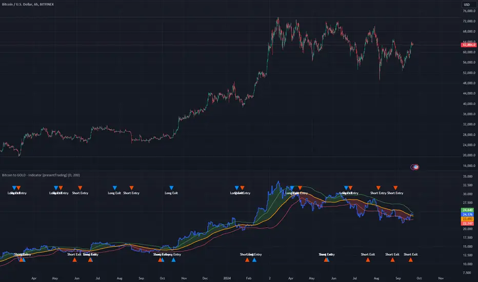
Bitcoin to GOLD [presentTrading]**Introduction and How it is Different**
Unlike traditional indicators, the BTGR offers a unique perspective on market sentiment and asset valuation by juxtaposing two seemingly disparate assets: Bitcoin, the digital gold, and Gold, the traditional store of value. This article introduces an advanced version of this ratio, complete with upper and lower bands calculated using standard deviations. These bands add an extra layer of analytical depth, allowing for more nuanced trading strategies.
BTCUSD 12h bigger picture
**Economic Principles**
The BTGR is rooted in the economic principles of asset valuation and market sentiment. Gold has long been considered a safe haven asset, a place where investors park their money during times of economic uncertainty. Bitcoin, on the other hand, is often viewed as a high-risk, high-reward investment. By comparing the two, the BTGR provides insights into the broader market sentiment.
- Risk Appetite: A high BTGR indicates a bullish sentiment towards riskier assets like Bitcoin.
- Market Uncertainty: A low BTGR suggests a bearish sentiment and a flight to the safety of Gold.
- Asset Diversification: The BTGR can be used as a tool for portfolio diversification, helping investors balance risk and reward.
**How to Use It**
Setting Up the Indicator
- Platform: The indicator is designed for use on TradingView.
- Time Frame: A 480-minute time frame is recommended for more accurate signals.
- Parameters: The moving average is set at 200 periods, and the standard deviation is calculated over the same period.
**Trading Signal**
Long Entry: Consider going long when the BTGR crosses above the upper band.
Short Entry: Consider going short when the BTGR crosses below the lower band.
Note: Due to the issue that the number of trading is less than about 100 times, the corresponding strategy is not allowed to publish.
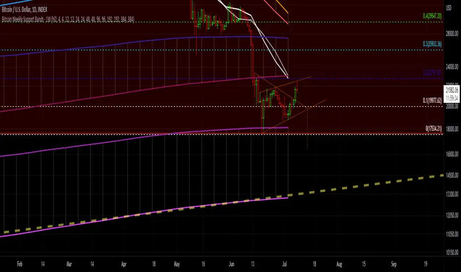
Bitcoin Support BandsSMA and EMA support/resistance bands for Bitcoin. Based on 4 week multiples; 1 month, 3 month, 6 month, 1 year, 2 year, 4 year.
Bitcoin Power Law Bands (BTC Power Law) Indicator█ OVERVIEW
The 'Bitcoin Power Law Bands' indicator is a set of three US dollar price trendlines and two price bands for bitcoin , indicating overall long-term trend, support and resistance levels as well as oversold and overbought conditions. The magnitude and growth of the middle (Center) line is determined by double logarithmic (log-log) regression on the entire USD price history of bitcoin . The upper (Resistance) and lower (Support) lines follow the same trajectory but multiplied by respective (fixed) factors. These two lines indicate levels where the price of bitcoin is expected to meet strong long-term resistance or receive strong long-term support. The two bands between the three lines are price levels where bitcoin may be considered overbought or oversold.
All parameters and visuals may be customized by the user as needed.
█ CONCEPTS
Long-term models
Long-term price models have many challenges, the most significant of which is getting the growth curve right overall. No one can predict how a certain market, asset class, or financial instrument will unfold over several decades. In the case of bitcoin , price history is very limited and extremely volatile, and this further complicates the situation. Fortunately for us, a few smart people already had some bright ideas that seem to have stood the test of time.
Power law
The so-called power law is the only long-term bitcoin price model that has a chance of survival for the years ahead. The idea behind the power law is very simple: over time, the rapid (exponential) initial growth cannot possibly be sustained (see The seduction of the exponential curve for a fun take on this). Year-on-year returns, therefore, must decrease over time, which leads us to the concept of diminishing returns and the power law. In this context, the power law translates to linear growth on a chart with both its axes scaled logarithmically. This is called the log-log chart (as opposed to the semilog chart you see above, on which only one of the axes - price - is logarithmic).
Log-log regression
When both price and time are scaled logarithmically, the power law leads to a linear relationship between them. This in turn allows us to apply linear regression techniques, which will find the best-fitting straight line to the data points in question. The result of performing this log-log regression (i.e. linear regression on a log-log scaled dataset) is two parameters: slope (m) and intercept (b). These parameters fully describe the relationship between price and time as follows: log(P) = m * log(T) + b, where P is price and T is time. Price is measured in US dollars , and Time is counted as the number of days elapsed since bitcoin 's genesis block.
DPC model
The final piece of our puzzle is the Dynamic Power Cycle (DPC) price model of bitcoin . DPC is a long-term cyclic model that uses the power law as its foundation, to which a periodic component stemming from the block subsidy halving cycle is applied dynamically. The regression parameters of this model are re-calculated daily to ensure longevity. For the 'Bitcoin Power Law Bands' indicator, the slope and intercept parameters were calculated on publication date (March 6, 2022). The slope of the Resistance Line is the same as that of the Center Line; its intercept was determined by fitting the line onto the Nov 2021 cycle peak. The slope of the Support Line is the same as that of the Center Line; its intercept was determined by fitting the line onto the Dec 2018 trough of the previous cycle. Please see the Limitations section below on the implications of a static model.
█ FEATURES
Inputs
• Parameters
• Center Intercept (b) and Slope (m): These log-log regression parameters control the behavior of the grey line in the middle
• Resistance Intercept (b) and Slope (m): These log-log regression parameters control the behavior of the red line at the top
• Support Intercept (b) and Slope (m): These log-log regression parameters control the behavior of the green line at the bottom
• Controls
• Plot Line Fill: N/A
• Plot Opportunity Label: Controls the display of current price level relative to the Center, Resistance and Support Lines
Style
• Visuals
• Center: Control, color, opacity, thickness, price line control and line style of the Center Line
• Resistance: Control, color, opacity, thickness, price line control and line style of the Resistance Line
• Support: Control, color, opacity, thickness, price line control and line style of the Support Line
• Plots Background: Control, color and opacity of the Upper Band
• Plots Background: Control, color and opacity of the Lower Band
• Labels: N/A
• Output
• Labels on price scale: Controls the display of current Center, Resistance and Support Line values on the price scale
• Values in status line: Controls the display of current Center, Resistance and Support Line values in the indicator's status line
█ HOW TO USE
The indicator includes three price lines:
• The grey Center Line in the middle shows the overall long-term bitcoin USD price trend
• The red Resistance Line at the top is an indication of where the bitcoin USD price is expected to meet strong long-term resistance
• The green Support Line at the bottom is an indication of where the bitcoin USD price is expected to receive strong long-term support
These lines envelope two price bands:
• The red Upper Band between the Center and Resistance Lines is an area where bitcoin is considered overbought (i.e. too expensive)
• The green Lower Band between the Support and Center Lines is an area where bitcoin is considered oversold (i.e. too cheap)
The power law model assumes that the price of bitcoin will fluctuate around the Center Line, by meeting resistance at the Resistance Line and finding support at the Support Line. When the current price is well below the Center Line (i.e. well into the green Lower Band), bitcoin is considered too cheap (oversold). When the current price is well above the Center Line (i.e. well into the red Upper Band), bitcoin is considered too expensive (overbought). This idea alone is not sufficient for profitable trading, but, when combined with other factors, it could guide the user's decision-making process in the right direction.
█ LIMITATIONS
The indicator is based on a static model, and for this reason it will gradually lose its usefulness. The Center Line is the most durable of the three lines since the long-term growth trend of bitcoin seems to deviate little from the power law. However, how far price extends above and below this line will change with every halving cycle (as can be seen for past cycles). Periodic updates will be needed to keep the indicator relevant. The user is invited to adjust the slope and intercept parameters manually between two updates of the indicator.
█ RAMBLINGS
The 'Bitcoin Power Law Bands' indicator is a useful tool for users wishing to place bitcoin in a macro context. As described above, the price level relative to the three lines is a rough indication of whether bitcoin is over- or undervalued. Users wishing to gain more insight into bitcoin price trends may follow the author's periodic updates of the DPC model (contact information below).
█ NOTES
The author regularly posts on Twitter using the @DeFi_initiate handle.
█ THANKS
Many thanks to the following individuals, who - one way or another - made the 'Bitcoin Power Law Bands' indicator possible:
• TradingView user 'capriole_charles', whose open-source 'Bitcoin Power Law Corridor' script was the basis for this indicator
• Harold Christopher Burger, whose Bitcoin’s natural long-term power-law corridor of growth article (2019) was the basis for the 'Bitcoin Power Law Corridor' script
• Bitcoin Forum user "Trololo", who posted the original power law model at Logarithmic (non-linear) regression - Bitcoin estimated value (2014)

Bitcoin Difficult Model [ChuckBanger]Simple script that graphically represents the mining difficulty of Bitcoin. It is ment to be used as a tool to decide when it is good time to dollar cost average (DCA) in your Bitcoin hodl position. When Price is below the difficulty model it is usually a good time to DCA.
Formula for the model used in this calculation is 0.002 * difficulty ^ 0.51. It is possible to change this numbers if necessarily.

Bitcoin Logarithmic Growth CurvesThis plots logarithmic curves fitted to major Bitcoin bear market tops & bottoms. Top line is fitted to bull tops, bottom line is fitted to lower areas of the logarithmic price trend (which is not always the same as bear market bottoms). Middle line is the median of the top & bottom, and the faded solid lines are fibonacci levels in between.
Inspired by & based on a Medium post by Harold Christopher Burger, which shows how linear Bitcoin's long-term price growth is when plotted on a double-log chart (log scaling on the price AND time axis).
These curves will only make sense for tickers representing Bitcoin vs. USD (such as BITSTAMP:BTCUSD, BITMEX:XBTUSD, BLX index). Plotting on other assets will probably end up with lines that shoot off into space without any relationship to the underlying price action.
The upper, middle & lower curves can be projected into the future, which can be turned on or off in the indicator settings. The fibonacci levels can also be switched on/off. And the upper & lower curve intercepts & slopes can be tweaked.
I'm releasing this open-source, if you end up making something cool based off of this code, I don't need attribution but please hit me up on here or on twitter (same username) so I can check out what ya made. Thanks, hope y'all enjoy it.

Bitcoin Halving Cycles [DotGain]Halving Cycles
A lightweight, time-anchored Bitcoin halving cycle visualizer built for clean charting, repeatable process planning, and simple profit/DCA timing references.
This Code was heavily inspired by KevinSvenson_ who created Bitcoin Halving Cycle Profit .
What this indicator does
This script plots the key “cycle landmarks” relative to each halving date:
Halving (⛏) – the cycle anchor
Profit START – marks the beginning of the post-halving profit window (default: 40 weeks )
Profit END / Last Call – marks the final phase of the profit window (default: 77 weeks )
DCA START – marks the point where long-term accumulation becomes the focus again (default: 135 weeks )
How to read it
Vertical lines = the exact cycle milestones
Bottom labels = description of each milestone aligned to its line (keeps the chart clean)
Green background (optional) = active Profit Zone on existing bars
Red background (optional) = optional warning zone after Profit END
HUD Panel (top-right)
The HUD gives you a fast “where are we in the cycle?” view with two modes:
Current Cycle
Shows: Halving date, Weeks since, and time remaining to Profit START / Last Call / DCA START within the current cycle.
Next Halving (Projection)
Shows: Countdown to the next enabled future halving, plus the projected weeks from today to Profit START / Last Call / DCA START after that future halving.
Future Halvings (manual)
You can manually add up to 3 future halving dates (Halving #1–#3).
This is useful for forward planning and cycle projection even before the event happens.
Enable Halving #1 / #2 / #3
Set Year / Month / Day for each
Optional: show/hide future markers & projections
Note: background zones only shade existing bars . Future projections are shown via lines/labels.
Settings overview
Show all cycles – plots every enabled cycle (historical + optional future). If disabled, only the current cycle is drawn.
Show Profit Zone background – green shading during the active profit window (current cycle only).
Show vertical markers + labels – toggles all milestone lines + labels.
Show HUD – toggles the HUD panel.
HUD Mode – switch between Current Cycle and Next Halving (Projection).
Cycle Logic – edit offsets in weeks (Profit START / Profit END / DCA START).
Optional Warning Zone – show a post-profit warning shading for a chosen number of weeks.
Have fun :)
Disclaimer
This Halving Cycles indicator is provided for informational and educational purposes only. It does not, and should not be construed as, financial, investment, or trading advice.
This indicator is an independent implementation of a time-based Bitcoin halving cycle visualization tool and is not affiliated with, or endorsed by, any third-party trading systems, strategies, protocols, or trademarked methodologies. The cycle zones, milestone markers, and countdown values displayed by this indicator are generated by a predefined set of algorithmic rules based on historical halving dates and user-defined time offsets. They do not constitute a direct recommendation to buy, sell, or hold any financial instrument or digital asset.
All trading and investing in financial markets involves a substantial risk of loss. You may lose part or all of your invested capital. Past performance does not guarantee future results. This indicator highlights historical and projected time-based market cycles and may produce false, lagging, incomplete, or misleading signals. Market behavior is influenced by many external factors and can deviate significantly from historical patterns or expectations.
The creator DotGain assumes no responsibility or liability for any financial losses, damages, or decisions made based on the use of this indicator or the information it provides. You are solely responsible for your own trading and investment decisions. Always conduct your own research (DYOR), use proper risk management, validate insights with additional tools or analysis, and consider your personal financial situation and risk tolerance before making any financial decision.

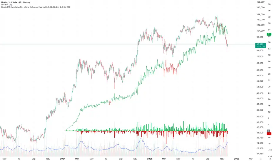
Bitcoin ETF Cumulative Net InflowIndicator Description:
This indicator calculates and plots the cumulative net inflow (in billions of USD) for selected Bitcoin ETFs on the main price chart. It uses AUM data from TradingView to estimate daily net flows, adjusted for BTC price changes, and accumulates them over time. The line is overlaid on the price chart (e.g., BTCUSD) with a right scale for better visibility, helping to identify correlations between ETF inflows and Bitcoin price movements.
Key Features:
Supports selection of 10 major Bitcoin ETFs (IBIT, FBTC, ARKB, etc.) via inputs.
Cumulative inflow line (purple, linewidth=2) for trend analysis.
Data sourced from request.financial("AUM", "D") for accuracy.
Bitcoin Cycle History Visualization [SwissAlgo]BTC 4-Year Cycle Tops & Bottoms
Historical visualization of Bitcoin's market cycles from 2010 to present, with projections based on weighted averages of past performance.
-----------------------------------------------------------------
CALCULATION METHODOLOGY
Why Bottom-to-Bottom Cycle Measurement?
This indicator defines cycles as bottom-to-bottom periods. This is one of several valid approaches to Bitcoin cycle analysis:
- Focuses on market behavior (price bottoms) rather than supply schedule events (halving-to-halving)
- Bottoms may offer good reference points for some analytical purposes
- Tops tend to be extended periods that are harder to define precisely
- Aligns with how some traditional asset cycles are measured and the timing observed in the broader "risk-on" assets category
- Halving events are shown separately (yellow backgrounds) for reference
- Neither halving-based nor bottom-based measurement is inherently superior
Different analysts prefer different cycle definitions based on their analytical goals. This approach prioritizes observable market turning points.
Cycle Date Definitions
- Approximate monthly ranges used for each event (e.g., Nov 2022 bottom = Nov 1-30, 2022)
- Cycle 1: Jul 2010 bottom → Jun 2011 top → Nov 2011 bottom
- Cycle 2: Nov 2011 bottom → Dec 2013 top → Jan 2015 bottom
- Cycle 3: Jan 2015 bottom → Dec 2017 top → Dec 2018 bottom
- Cycle 4: Dec 2018 bottom → Nov 2021 top → Nov 2022 bottom
- Future cycles will be added as new top/bottom dates become firm
Duration Calculations
- Days = timestamp difference converted to days (milliseconds ÷ 86,400,000)
- Bottom → Top: days from cycle bottom to peak
- Top → Bottom: days from peak to next cycle bottom
- Bottom → Bottom: full cycle duration (sum of above)
Price Change Calculations
- % Change = ((New Price - Old Price) / Old Price) × 100
- Example: $200 → $19,700 = ((19,700 - 200) / 200) × 100 = 9,750% gain
- Approximate historical prices used (rounded to significant figures)
Weighted Average Formula
Recent cycles weighted more heavily to reflect the evolved market structure:
- Cycle 1 (2010-2011): EXCLUDED (too early-stage, tiny market cap)
- Cycle 2 (2011-2015): Weight = 1x
- Cycle 3 (2015-2018): Weight = 3x
- Cycle 4 (2018-2022): Weight = 5x
Formula: Weighted Avg = (C2×1 + C3×3 + C4×5) / (1+3+5)
Example for Bottom→Top days: (761×1 + 1065×3 + 1066×5) / 9 = 1,032 days
Projection Method
- Projected Top Date = Nov 2022 bottom + weighted avg Bottom→Top days
- Projected Bottom Date = Nov 2022 bottom + weighted avg Bottom→Bottom days
- Current days elapsed compared to weighted averages
- Warning symbol (⚠) shown when the current cycle exceeds the historical average
Technical Implementation
- Historical cycle dates are hardcoded (not algorithmically detected)
- Dates represent approximate monthly ranges for each event
- The indicator will be updated as the Cycle 5 top and bottom dates become confirmed
- Updates require manual code maintenance - not automatic
- Users should verify they're using the latest version for current cycle data
-----------------------------------------------------------------
FEATURES
- Background highlights for historical tops (red), bottoms (green), and halving events (yellow)
- Data table showing cycle durations and price changes
- Visual cycle boundary boxes with subtle coloring
- Projected timeframes displayed as dashed vertical lines
- Toggle on/off for each visual element
- Customizable background colors
-----------------------------------------------------------------
DISPLAY SETTINGS
- Show/hide cycle tops, bottoms, halvings, data table, and cycle boxes
- Customizable background colors for each event type
- Clean, institutional-grade visual design suitable for analysis
UPDATES & MAINTENANCE
This indicator is maintained as new cycle events occur. When Cycle 5's top and bottom are confirmed with sufficient time elapsed, the code and projections will be updated accordingly. Check for the latest version periodically.
OPEN SOURCE
Code available for review, modification, and improvement. Educational transparency is prioritized.
-----------------------------------------------------------------
IMPORTANT LIMITATIONS
⚠ EXTREMELY SMALL SAMPLE SIZE
Based on only 4 complete cycles (2011-2022). In statistical analysis, this is insufficient for reliable predictions.
⚠ CHANGED MARKET STRUCTURE
Bitcoin's market has fundamentally evolved since early cycles:
- 2010-2015: Tiny market cap, retail-only, unregulated
- 2024-2025: Institutional adoption, spot ETFs, regulatory frameworks, macro correlation
The environment that created past patterns no longer exists in the same form.
⚠ NO PREDICTIVE GUARANTEE
Historical patterns can and do break. Market cycles are not laws of physics. Past performance does not guarantee future results. The next cycle may not follow historical averages.
⚠ LENGTHENING CYCLE THEORY
Some analysts believe cycles are extending over time (diminishing returns, maturing market). If true, simple averaging underestimates future cycle lengths.
⚠ SELF-FULFILLING PROPHECY RISK
The halving narrative may be partially circular - it works because people believe it works. Sufficient changes in market structure or participant behavior can invalidate the pattern.
⚠ APPROXIMATE DATA
Historical prices rounded to significant figures. Exact bottom/top dates vary by exchange. Month-long ranges are used for simplicity.
EDUCATIONAL USE ONLY
This indicator is designed for historical analysis and understanding Bitcoin's past behavior. It is NOT:
- Trading advice or financial recommendations
- A guarantee or prediction of future price movements
- Suitable as a sole basis for investment decisions
- A replacement for fundamental or technical analysis
The projections show "what if the pattern continues exactly" - not "what will happen."
Always conduct independent research, understand the risks, and consult qualified financial advisors before making investment decisions. Only invest what you can afford to lose.

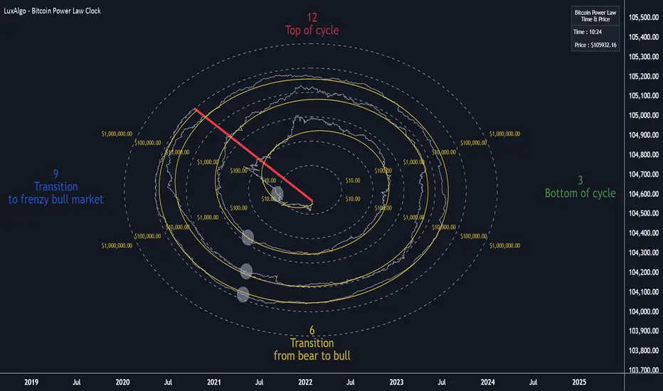
Bitcoin Power Law Clock [LuxAlgo]The Bitcoin Power Law Clock is a unique representation of Bitcoin prices proposed by famous Bitcoin analyst and modeler Giovanni Santostasi.
It displays a clock-like figure with the Bitcoin price and average lines as spirals, as well as the 12, 3, 6, and 9 hour marks as key points in the cycle.
🔶 USAGE
Giovanni Santostasi, Ph.D., is the creator and discoverer of the Bitcoin Power Law Theory. He is passionate about Bitcoin and has 12 years of experience analyzing it and creating price models.
As we can see in the above chart, the tool is super intuitive. It displays a clock-like figure with the current Bitcoin price at 10:20 on a 12-hour scale.
This tool only works on the 1D INDEX:BTCUSD chart. The ticker and timeframe must be exact to ensure proper functionality.
According to the Bitcoin Power Law Theory, the key cycle points are marked at the extremes of the clock: 12, 3, 6, and 9 hours. According to the theory, the current Bitcoin prices are in a frenzied bull market on their way to the top of the cycle.
🔹 Enable/Disable Elements
All of the elements on the clock can be disabled. If you disable them all, only an empty space will remain.
The different charts above show various combinations. Traders can customize the tool to their needs.
🔹 Auto scale
The clock has an auto-scale feature that is enabled by default. Traders can adjust the size of the clock by disabling this feature and setting the size in the settings panel.
The image above shows different configurations of this feature.
🔶 SETTINGS
🔹 Price
Price: Enable/disable price spiral, select color, and enable/disable curved mode
Average: Enable/disable average spiral, select color, and enable/disable curved mode
🔹 Style
Auto scale: Enable/disable automatic scaling or set manual fixed scaling for the spirals
Lines width: Width of each spiral line
Text Size: Select text size for date tags and price scales
Prices: Enable/disable price scales on the x-axis
Handle: Enable/disable clock handle
Halvings: Enable/disable Halvings
Hours: Enable/disable hours and key cycle points
🔹 Time & Price Dashboard
Show Time & Price: Enable/disable time & price dashboard
Location: Dashboard location
Size: Dashboard size
Bitcoin Power Law OscillatorThis is the oscillator version of the script. The main body of the script can be found here.
Understanding the Bitcoin Power Law Model
Also called the Long-Term Bitcoin Power Law Model. The Bitcoin Power Law model tries to capture and predict Bitcoin's price growth over time. It assumes that Bitcoin's price follows an exponential growth pattern, where the price increases over time according to a mathematical relationship.
By fitting a power law to historical data, the model creates a trend line that represents this growth. It then generates additional parallel lines (support and resistance lines) to show potential price boundaries, helping to visualize where Bitcoin’s price could move within certain ranges.
In simple terms, the model helps us understand Bitcoin's general growth trajectory and provides a framework to visualize how its price could behave over the long term.
The Bitcoin Power Law has the following function:
Power Law = 10^(a + b * log10(d))
Consisting of the following parameters:
a: Power Law Intercept (default: -17.668).
b: Power Law Slope (default: 5.926).
d: Number of days since a reference point(calculated by counting bars from the reference point with an offset).
Explanation of the a and b parameters:
Roughly explained, the optimal values for the a and b parameters are determined through a process of linear regression on a log-log scale (after applying a logarithmic transformation to both the x and y axes). On this log-log scale, the power law relationship becomes linear, making it possible to apply linear regression. The best fit for the regression is then evaluated using metrics like the R-squared value, residual error analysis, and visual inspection. This process can be quite complex and is beyond the scope of this post.
Applying vertical shifts to generate the other lines:
Once the initial power-law is created, additional lines are generated by applying a vertical shift. This shift is achieved by adding a specific number of days (or years in case of this script) to the d-parameter. This creates new lines perfectly parallel to the initial power law with an added vertical shift, maintaining the same slope and intercept.
In the case of this script, shifts are made by adding +365 days, +2 * 365 days, +3 * 365 days, +4 * 365 days, and +5 * 365 days, effectively introducing one to five years of shifts. This results in a total of six Power Law lines, as outlined below (From lowest to highest):
Base Power Law Line (no shift)
1-year shifted line
2-year shifted line
3-year shifted line
4-year shifted line
5-year shifted line
The six power law lines:
Bitcoin Power Law Oscillator
This publication also includes the oscillator version of the Bitcoin Power Law. This version applies a logarithmic transformation to the price, Base Power Law Line, and 5-year shifted line using the formula: log10(x) .
The log-transformed price is then normalized using min-max normalization relative to the log-transformed Base Power Law Line and 5-year shifted line with the formula:
normalized price = log(close) - log(Base Power Law Line) / log(5-year shifted line) - log(Base Power Law Line)
Finally, the normalized price was multiplied by 5 to map its value between 0 and 5, aligning with the shifted lines.
Interpretation of the Bitcoin Power Law Model:
The shifted Power Law lines provide a framework for predicting Bitcoin's future price movements based on historical trends. These lines are created by applying a vertical shift to the initial Power Law line, with each shifted line representing a future time frame (e.g., 1 year, 2 years, 3 years, etc.).
By analyzing these shifted lines, users can make predictions about minimum price levels at specific future dates. For example, the 5-year shifted line will act as the main support level for Bitcoin’s price in 5 years, meaning that Bitcoin’s price should not fall below this line, ensuring that Bitcoin will be valued at least at this level by that time. Similarly, the 2-year shifted line will serve as the support line for Bitcoin's price in 2 years, establishing that the price should not drop below this line within that time frame.
On the other hand, the 5-year shifted line also functions as an absolute resistance , meaning Bitcoin's price will not exceed this line prior to the 5-year mark. This provides a prediction that Bitcoin cannot reach certain price levels before a specific date. For example, the price of Bitcoin is unlikely to reach $100,000 before 2021, and it will not exceed this price before the 5-year shifted line becomes relevant. After 2028, however, the price is predicted to never fall below $100,000, thanks to the support established by the shifted lines.
In essence, the shifted Power Law lines offer a way to predict both the minimum price levels that Bitcoin will hit by certain dates and the earliest dates by which certain price points will be reached. These lines help frame Bitcoin's potential future price range, offering insight into long-term price behavior and providing a guide for investors and analysts. Lets examine some examples:
Example 1:
In Example 1 it can be seen that point A on the 5-year shifted line acts as major resistance . Also it can be seen that 5 years later this price level now corresponds to the Base Power Law Line and acts as a major support at point B(Note: Vertical yearly grid lines have been added for this purpose👍).
Example 2:
In Example 2, the price level at point C on the 3-year shifted line becomes a major support three years later at point D, now aligning with the Base Power Law Line.
Finally, let's explore some future price predictions, as this script provides projections on the weekly timeframe :
Example 3:
In Example 3, the Bitcoin Power Law indicates that Bitcoin's price cannot surpass approximately $808K before 2030 as can be seen at point E, while also ensuring it will be at least $224K by then (point F).

Bitcoin Power LawThis is the main body version of the script. The Oscillator version can be found here.
Understanding the Bitcoin Power Law Model
Also called the Long-Term Bitcoin Power Law Model. The Bitcoin Power Law model tries to capture and predict Bitcoin's price growth over time. It assumes that Bitcoin's price follows an exponential growth pattern, where the price increases over time according to a mathematical relationship.
By fitting a power law to historical data, the model creates a trend line that represents this growth. It then generates additional parallel lines (support and resistance lines) to show potential price boundaries, helping to visualize where Bitcoin’s price could move within certain ranges.
In simple terms, the model helps us understand Bitcoin's general growth trajectory and provides a framework to visualize how its price could behave over the long term.
The Bitcoin Power Law has the following function:
Power Law = 10^(a + b * log10(d))
Consisting of the following parameters:
a: Power Law Intercept (default: -17.668).
b: Power Law Slope (default: 5.926).
d: Number of days since a reference point(calculated by counting bars from the reference point with an offset).
Explanation of the a and b parameters:
Roughly explained, the optimal values for the a and b parameters are determined through a process of linear regression on a log-log scale (after applying a logarithmic transformation to both the x and y axes). On this log-log scale, the power law relationship becomes linear, making it possible to apply linear regression. The best fit for the regression is then evaluated using metrics like the R-squared value, residual error analysis, and visual inspection. This process can be quite complex and is beyond the scope of this post.
Applying vertical shifts to generate the other lines:
Once the initial power-law is created, additional lines are generated by applying a vertical shift. This shift is achieved by adding a specific number of days (or years in case of this script) to the d-parameter. This creates new lines perfectly parallel to the initial power law with an added vertical shift, maintaining the same slope and intercept.
In the case of this script, shifts are made by adding +365 days, +2 * 365 days, +3 * 365 days, +4 * 365 days, and +5 * 365 days, effectively introducing one to five years of shifts. This results in a total of six Power Law lines, as outlined below (From lowest to highest):
Base Power Law Line (no shift)
1-year shifted line
2-year shifted line
3-year shifted line
4-year shifted line
5-year shifted line
The six power law lines:
Bitcoin Power Law Oscillator
This publication also includes the oscillator version of the Bitcoin Power Law. This version applies a logarithmic transformation to the price, Base Power Law Line, and 5-year shifted line using the formula: log10(x) .
The log-transformed price is then normalized using min-max normalization relative to the log-transformed Base Power Law Line and 5-year shifted line with the formula:
normalized price = log(close) - log(Base Power Law Line) / log(5-year shifted line) - log(Base Power Law Line)
Finally, the normalized price was multiplied by 5 to map its value between 0 and 5, aligning with the shifted lines.
Interpretation of the Bitcoin Power Law Model:
The shifted Power Law lines provide a framework for predicting Bitcoin's future price movements based on historical trends. These lines are created by applying a vertical shift to the initial Power Law line, with each shifted line representing a future time frame (e.g., 1 year, 2 years, 3 years, etc.).
By analyzing these shifted lines, users can make predictions about minimum price levels at specific future dates. For example, the 5-year shifted line will act as the main support level for Bitcoin’s price in 5 years, meaning that Bitcoin’s price should not fall below this line, ensuring that Bitcoin will be valued at least at this level by that time. Similarly, the 2-year shifted line will serve as the support line for Bitcoin's price in 2 years, establishing that the price should not drop below this line within that time frame.
On the other hand, the 5-year shifted line also functions as an absolute resistance , meaning Bitcoin's price will not exceed this line prior to the 5-year mark. This provides a prediction that Bitcoin cannot reach certain price levels before a specific date. For example, the price of Bitcoin is unlikely to reach $100,000 before 2021, and it will not exceed this price before the 5-year shifted line becomes relevant. After 2028, however, the price is predicted to never fall below $100,000, thanks to the support established by the shifted lines.
In essence, the shifted Power Law lines offer a way to predict both the minimum price levels that Bitcoin will hit by certain dates and the earliest dates by which certain price points will be reached. These lines help frame Bitcoin's potential future price range, offering insight into long-term price behavior and providing a guide for investors and analysts. Lets examine some examples:
Example 1:
In Example 1 it can be seen that point A on the 5-year shifted line acts as major resistance . Also it can be seen that 5 years later this price level now corresponds to the Base Power Law Line and acts as a major support at point B (Note: Vertical yearly grid lines have been added for this purpose👍).
Example 2:
In Example 2, the price level at point C on the 3-year shifted line becomes a major support three years later at point D, now aligning with the Base Power Law Line.
Finally, let's explore some future price predictions, as this script provides projections on the weekly timeframe :
Example 3:
In Example 3, the Bitcoin Power Law indicates that Bitcoin's price cannot surpass approximately $808K before 2030 as can be seen at point E, while also ensuring it will be at least $224K by then (point F).
