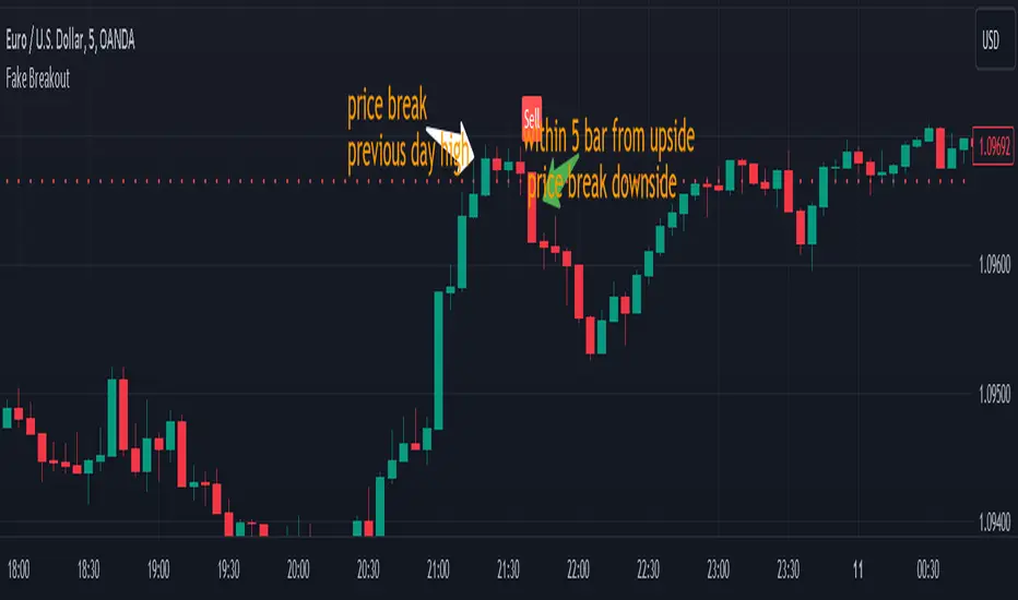
Pivot Data [QuantVue]The Pivot Data Indicator is designed to provide traders with valuable insights by identifying and analyzing pivot points on the price chart. It calculates both pivot highs and lows, then presents detailed statistics on the distance and time between these pivots.
a pivot point is defined as a specific point on the chart where the price either reaches a high or a low, with no bars higher or lower than it for a set number of bars on both sides (left and right). Essentially, it's a local high or low point, with the market moving in the opposite direction after the pivot forms.
For example:
A pivot high occurs when there are no bars with higher prices for a specified number of bars before and after that point.
A pivot low occurs when there are no bars with lower prices for the same number of bars on either side.
The number of bars to the left and right is adjustable via the Pivot Lookback Bars setting, allowing you to define how many bars are used to determine these pivot points.
Key features include:
Pivot Highs and Lows Identification: Automatically marks significant pivot highs and lows based on a user-defined lookback period, helping traders identify potential trend reversals or continuation points.
Prediction Labels: Provides forecasted pivot levels based on historical pivot price and time patterns, with options to show predictions for pivot highs, lows, or any pivot point.
Customizable Table Display: Displays a table summarizing important statistics, such as the average price percentage and the number of bars between pivots, along with the distance and time from the most recent pivot.
Traders can use this tool to map out potential levels of support and resistance based on historical data on pivot points.
在腳本中搜尋"high low"
Internal Bar Strength IBS [Anan]This indicator calculates and displays the Internal Bar Strength (IBS) along with its moving average. The IBS is a measure that represents where the closing price is relative to the high-low range of a given period.
█ Main Formula
The core of this indicator is the Internal Bar Strength (IBS) calculation. The basic IBS formula is:
ibs = (close - low) / (high - low)
I enhanced the original formula by incorporating a user-defined length parameter. This modification allows for greater flexibility in analysis and interpretation. The extended version enables users to adjust the indicator's length according to their specific needs or market conditions. Notably, setting the length parameter to 1 reproduces the behavior of the original formula, maintaining backward compatibility while offering expanded functionality:
ibs = (close - ta.lowest(low, ibs_length)) / (ta.highest(high, ibs_length) - ta.lowest(low, ibs_length))
Where:
- `close` is the closing price of the current bar
- `lowest low` is the lowest low price over the specified IBS length
- `highest high` is the highest high price over the specified IBS length
█ Key Features
- Calculates IBS using a user-defined length
- Applies a moving average to the IBS values
- Offers multiple moving average types
- Includes optional Bollinger Bands or Donchian Channel overlays
- Visualizes bull and bear areas
█ Inputs
- IBS Length: The period used for IBS calculation
- MA Type: The type of moving average applied to IBS (options: SMA, EMA, SMMA, WMA, VWMA, Bollinger Bands, Donchian)
- MA Length: The period used for the moving average calculation
- BB StdDev: Standard deviation multiplier for Bollinger Bands
█ How to Use and Interpret
1. IBS Line Interpretation:
- IBS values range from 0 to 1
- Values close to 1 indicate the close was near the high, suggesting a bullish sentiment
- Values close to 0 indicate the close was near the low, suggesting a bearish sentiment
- Values around 0.5 suggest the close was near the middle of the range
2. Overbought/Oversold Conditions:
- IBS values above 0.8 (teal zone) may indicate overbought conditions
- IBS values below 0.2 (red zone) may indicate oversold conditions
- These zones can be used to identify potential reversal points
3. Trend Identification:
- Consistent IBS values above 0.5 may indicate an uptrend
- Consistent IBS values below 0.5 may indicate a downtrend
4. Using Moving Averages:
- The yellow MA line can help smooth out IBS fluctuations
- Crossovers between the IBS and its MA can signal potential trend changes
5. Bollinger Bands/Donchian Channel:
- When enabled, these can provide additional context for overbought/oversold conditions
- IBS touching or exceeding the upper band may indicate overbought conditions
- IBS touching or falling below the lower band may indicate oversold conditions
Remember that no single indicator should be used in isolation. Always combine IBS analysis with other technical indicators, price action analysis, and broader market context for more reliable trading decisions.
Dynamic Support & Resistance Tracker with MTFDynamic Support & Resistance Tracker with Weekly, Monthly & Daily Levels
The Dynamic Support & Resistance Tracker is designed to help traders identify key support and resistance levels across multiple timeframes, enhancing market analysis and decision-making. This indicator calculates and plots support and resistance levels for daily, weekly, and monthly periods, along with extension lines that provide insights into potential price targets.
Key Features:
Multi-Timeframe Analysis:
Daily Levels: Identifies the high, low, and midpoint for each trading day. These levels help traders recognize important price points for short-term trading strategies.
Weekly Levels: Plots the high, low, and midpoint for each week. This feature is valuable for swing traders who need to understand broader market trends.
Monthly Levels: Displays the high, low, and midpoint for each month, which is essential for long-term investors.
Extension Lines:
Calculates extension lines beyond the standard support and resistance levels to help anticipate potential price targets and reversals. These extensions are based on the distance between the high/low and midpoint levels.
Real-Time Updates:
Automatically updates the levels based on the most recent market data, ensuring traders have the most current information for their analysis.
Clear Visuals:
The indicator provides clearly labeled and color-coded lines for easy identification of key levels, improving the visual clarity of market analysis.
How It Works:
Daily, Weekly, and Monthly Levels: The indicator calculates the high, low, and midpoint levels for daily, weekly, and monthly timeframes and plots them on the chart. These levels serve as potential areas of support and resistance where price action may react.
Extension Lines: The extension lines are calculated based on the distance between the high/low and midpoint levels, projecting potential areas where price may find support or resistance beyond the standard levels.
Automatic Updates: The indicator continuously updates the plotted levels based on the latest market data, providing real-time insights.
Benefits:
Improved Market Analysis: By providing a clear view of support and resistance levels across multiple timeframes, this indicator helps traders understand market trends and price movements more effectively.
Informed Trading Decisions: The detailed plotting of levels and extensions allows traders to make more informed decisions, enhancing their trading strategies.
Versatility: Suitable for various trading styles, including intraday trading, swing trading, and long-term investing.
Instructions for Use:
Analyze the Levels: Observe the plotted high, low, and mid-levels for daily, weekly, and monthly timeframes.
Plan Your Trades: Use the identified support and resistance levels to set your entry and exit points, stop-losses, and profit targets.
Monitor the Market: Stay updated with real-time adjustments of the levels, ensuring you always have the latest market information.
Note: This indicator is designed to enhance your trading analysis by providing clear and reliable support and resistance levels. However, it should be used as part of a comprehensive trading strategy and not as the sole basis for trading decisions.
Reversal Zones with SignalsThe "Reversal Zones with Signals" indicator is an advanced technical analysis tool designed to help traders identify potential market reversal points. By integrating Relative Strength Index (RSI), moving averages, and swing high/low detection, this indicator provides traders with clear visual cues for potential buy and sell opportunities.
Key Features and Benefits
Integration of Multiple Technical Analysis Tools:
The indicator seamlessly combines RSI, moving averages, and swing high/low detection. This multi-faceted approach enhances the reliability of the signals by confirming potential reversals through different technical analysis perspectives.
Customizable Parameters:
Users can adjust the sensitivity of the moving averages, the RSI overbought and oversold levels, and the length of the reversal zones. This flexibility allows traders to tailor the indicator to fit their specific trading strategies and market conditions.
Clear Visual Signals:
Buy and sell signals are plotted directly on the chart as easily recognizable green and red labels. This visual clarity simplifies the process of identifying potential entry and exit points, enabling traders to act quickly and decisively.
Reversal Zones:
The indicator plots reversal zones based on swing highs and lows in conjunction with RSI conditions. Green lines represent potential support levels (zone bottoms), while red lines represent potential resistance levels (zone tops). These zones provide traders with clear areas where price reversals are likely to occur.
Automated Alerts:
Custom alerts can be set for both buy and sell signals, providing real-time notifications when potential trading opportunities arise. This feature ensures that traders do not miss critical market moves.
How It Works
RSI Calculation:
The Relative Strength Index (RSI) is calculated to determine overbought and oversold conditions. When RSI exceeds the overbought threshold, it indicates that the market may be overbought, and when it falls below the oversold threshold, it indicates that the market may be oversold. This helps in identifying potential reversal points.
Swing High/Low Detection:
Swing highs and lows are detected using a specified lookback period. These points represent significant price levels where reversals are likely to occur. Swing highs are detected using the ta.pivothigh function, and swing lows are detected using the ta.pivotlow function.
Reversal Zones:
Reversal zones are defined by plotting lines at swing high and low levels when RSI conditions are met. These zones serve as visual cues for potential support and resistance areas, providing a structured framework for identifying reversal points.
Buy and Sell Signals:
Buy signals are generated when the price crosses above a defined reversal zone bottom, indicating a potential upward reversal. Sell signals are generated when the price crosses below a defined reversal zone top, indicating a potential downward reversal. These signals are further confirmed by the presence of bullish or bearish engulfing patterns.
Plotting and Alerts:
The indicator plots buy and sell signals directly on the chart with corresponding labels. Additionally, alerts can be set up to notify the user when a signal is generated, ensuring timely action.
Originality and Usefulness
Innovative Integration of Technical Tools:
The "Reversal Zones with Signals" indicator uniquely combines multiple technical analysis tools into a single, cohesive indicator. This integration provides a comprehensive view of market conditions, enhancing the accuracy of the signals and offering a robust tool for traders.
Enhanced Trading Decisions:
By providing clear and actionable signals, the indicator helps traders make better-informed decisions. The visualization of reversal zones and the integration of RSI and moving averages ensure that traders have a solid framework for identifying potential reversals.
Flexibility and Customization:
The customizable parameters allow traders to adapt the indicator to different trading styles and market conditions. This flexibility ensures that the indicator can be used effectively by a wide range of traders, from beginners to advanced professionals.
Clear and User-Friendly Interface:
The indicator's design prioritizes ease of use, with clear visual signals and intuitive settings. This user-friendly approach makes it accessible to traders of all experience levels.
Real-Time Alerts:
The ability to set up custom alerts ensures that traders are notified of potential trading opportunities as they arise, helping them to act quickly and efficiently.
Versatility Across Markets:
The indicator is suitable for use in various financial markets, including stocks, forex, and cryptocurrencies. Its adaptability across different asset classes makes it a valuable addition to any trader's toolkit.
How to Use
Adding the Indicator:
Add the "Reversal Zones with Signals" indicator to your chart.
Adjust the parameters (Sensitivity, RSI OverBought Value, RSI OverSold Value, Zone Length) to match your trading strategy and market conditions.
Interpreting Signals:
Buy Signal: A green "BUY" label appears below a bar, indicating a potential buying opportunity based on the detected reversal zone and price action.
Sell Signal: A red "SELL" label appears above a bar, indicating a potential selling opportunity based on the detected reversal zone and price action.
Setting Alerts:
Set alerts for buy and sell signals to receive notifications when potential trading opportunities arise. This ensures timely action and helps traders stay informed about critical market moves.
CPR by MTThe CPR indicator, or Central Pivot Range indicator, is a technical analysis tool used in trading to identify potential support and resistance levels based on the price action of a security. Developed by pivot point theory, it is particularly popular among day traders and swing traders. The CPR indicator consists of three lines:
1. **Pivot Point (PP):** This is the central line and is calculated as the average of the high, low, and closing prices from the previous trading period.
\
2. **Top Central Pivot (TC):** This is calculated by subtracting the low from the PP and then adding the result to the PP.
\
3. **Bottom Central Pivot (BC):** This is calculated by subtracting the high from the PP and then adding the result to the PP.
\
### How to Use the CPR Indicator
- **Trend Identification:** A wide CPR range indicates low volatility and a potential sideways or consolidation phase. A narrow CPR range indicates high volatility and a potential strong trending move.
- **Support and Resistance:** The top and bottom central pivots act as immediate resistance and support levels. If the price is above the TC, it indicates a bullish sentiment, while if it is below the BC, it indicates a bearish sentiment.
- **Entry and Exit Points:** Traders use the CPR lines to determine optimal entry and exit points. For example, if the price breaks above the TC and sustains, it may signal a buy opportunity, whereas a drop below the BC may signal a sell opportunity.
### Practical Example
Suppose a stock had a high of $105, a low of $95, and a closing price of $100 on the previous day. The CPR levels for the next day would be calculated as follows:
1. **Pivot Point (PP):**
\
2. **Top Central Pivot (TC):**
\
3. **Bottom Central Pivot (BC):**
\
The levels for the next day would be PP = $100, TC = $110, and BC = $90. Traders would then use these levels to assess potential trading strategies based on where the price moves relative to these levels.
### Conclusion
The CPR indicator is a useful tool for traders looking to understand market conditions and make informed decisions about entry and exit points. Its effectiveness comes from its ability to highlight key price levels derived from historical price data, helping traders predict potential market movements.
20,200SMA,PDHL,15 minute ORBSimple Moving Averages (SMAs):
The script calculates three SMAs: SMA 20 High, SMA 20 Low, and SMA 200 Close. These moving averages are widely used in technical analysis to smooth out price data and identify trends.
The SMA for the high price (SMA 20 High) is calculated based on the 20-period moving average of the high prices.
Similarly, the SMA for the low price (SMA 20 Low) is calculated based on the 20-period moving average of the low prices.
The SMA for the close price (SMA 200 Close) is calculated based on the 200-period moving average of the closing prices.
Each SMA is plotted on the chart, and their colors are determined based on whether the current close price is above or below each respective SMA.
Conditional Coloring:
The script employs conditional coloring to visually highlight whether the close price is above or below each SMA.
If the close price is below the SMA 20 High, it's plotted in red; otherwise, it's plotted in green.
Similarly, the SMA 20 Low and SMA 200 Close are plotted with conditional colors based on the relationship between the close price and each respective SMA.
Previous Day's Data:
The script retrieves and plots the high, low, and close prices of the previous trading day.
This provides traders with valuable information about the previous day's market behavior, which can influence trading decisions.
Opening 15-minute Range Breakout:
The script calculates the high and low prices during the first 15 minutes of each trading day.
These prices represent the opening range for the day.
It then determines whether the current close price is above or below this opening range and plots it accordingly.
This breakout strategy helps traders identify potential trading opportunities based on early price movements.
By integrating these components, the script offers traders a comprehensive analysis of market trends, previous day's performance, and potential breakout opportunities. Its originality lies in the combination of these features into a single, easy-to-use indicator, providing valuable insights for trading decisions.
yatsThis is a helper indicator for "yats" (Yet Another Trading Strategy).
This is a grouping of several indicators in one to help with a very basic trend following strategy. In order to utilize this indicator, it is best to have your chart set to a Line chart.
How to use:
This is a basic trend strategy in which the trader will enter or reverse their position on the break of the trend.
With the chart set to line and the source set to close, a basic line with peaks and valleys is displayed.
When the line peaks, then retreats, this is a potential setup for a long position. The trader is to wait for a valley (lower point) to be formed and then for the previous peak to be broken.
The timeframe continuity labels in the lower right of the chart help to ensure the position taken is in line with the higher timeframe trend.
Example scenario (long):
Chart is set to 1H timeframe. Timeframe continuity indicator will have labels for 1H, 4H, Day, WK, MN, and QTR. Chart shows a peak at a close price of 5 then the next bar sets a valley at a close price of 4.
Next bar forms and sets a close price of 6. Timeframe continuity labels are green for 1H, 4H, Day, and WK. (At least three higher timeframes should match the direction of the desired trade.)
This is a signal to go long as the previous peak was broken and timeframe continuity is in the direction
of the trade (long). Initial conservative stoploss should be placed at the previous valley (4). A wider stoploss could be placed at the low created when the close was 4. This is made visible by the default red line
when Candle Highs and Lows plots are turned on. Stoploss is then trailed up either by each subsequent higher low, OR with each subsequent dip as price moves higher.
A target can be set, but is not an integral part of this strategy.
Features:
Full Timeframe Continuity:
In the lower right corner of the chart will be indicators for timeframes greater than or equal to the chart timeframe.
Each one will be Red, Green, or White to indicate down, up, or flat. This provides you with the direction of the higher timeframes in real time, before the bar has closed.
Potential Support/Resistance Points:
The indicator plots horizontal rays for the previous Day, Week, and Month for the High, Low, and Close. Day = Orange, Week = White, Month = Purple. High and Low are solid lines while Close is a dashed line.
This provides the trader with potential pivot points based on higher timeframe high, low, and close prices. The horizontal rays will automatically move to the right at the start of the newest day, week, or month.
Candle Highs and Lows:
Since the chart should be set to Line instead of Candles or Bars, this indicator provides plots that follow the Highs (Green) and Lows (Red) of each 'bar' of the chart timeframe. This has been made configurable
so these lines can be turned off or edited in the settings for those who do not want them on the chart or just want them to look different.
swinglibraryLibrary "swinglibrary"
This library is for calculating non-repainting swings for further calculation on them.
These swings can later be drawn, but drawing is not part of this library, only the calculation.
What do I need to use the library?
You better include the following constants into your script using this library:
int SWING_NO_ACTION = 0
int SWING_FLIP = 1
int SWING_FLIP_NEW_SWING = 2
int SWING_FLIP_UPDATED = 3
int RELATION_HIGHER = 1
int RELATION_EQUAL = 0
int RELATION_LOWER = -1
Choosing the function, that fits your needs
This library contains 4 functions for calculating swings, the difference between them are the data you get for every swing point and additional average values for length and duration:
swings()
swingsR()
swingsL()
swingsLDR()
The naming scheme of these functions is the following:
The base version swings() is only for the swings containing the following swingPoint type:
swingPoint
Fields:
x (integer) : bar index
y (float) : price
hilo (integer) 1 -> high, -1 -> low
and the return type:
swingReturn
Fields:
swings (array) : array of the last x swing points
newSwingHigh (integer) : flag to detect changes for swing highs see constants (SWING_NO_ACTION, SWING_FLIP_NEW_SWING, SWING_FLIP_UPDATED)
newSwingLow (integer) : flag to detect changes for swing lows see constants (SWING_NO_ACTION, SWING_FLIP_NEW_SWING, SWING_FLIP_UPDATED)
The R in swingsR() stands for relation where the previously shown types do also contain the relation between the swings of the same swing type (highs and lows respectively).
The same goes for L in swingsL() for length containing the price difference between the current and previous swing point in ticks.
And in the following version swingsLDR() there is also the duration between the current and previous point included.
The parameters for the other functions and type definitions include only the ones, that are needed, the "full" version of the function is described here:
swingsLDR(swingSize, dtbStrength, init, SWING_HISTORY_NUM)
Parameters:
swingSize (int) This parameter defines the size of the swings to look after, meaning higher values will lead to bigger swings
dtbStrength (int) Value between 0 and 100 is a factor (%) to the ATR that is used to calculate equal highs/lows (double tops / bottoms).
Higher values will result in a higher tolerance of price difference between the swings.
init (bool) This value is usually set to false on default.
It has a special use case, where we need to reduce memory usage and calculation time on the script using this library by start calculating at x bars back instead of the beginning of the chart.
In this case, we set init = true on the first bar we start calculating the swings on to perform the correct initialization.
SWING_HISTORY_NUM (int) This is the max number of swings that are stored in the array, so only the last SWING_HISTORY_NUM swings are stored in the array to reduce the memory usage.
New ones remove the oldest ones like in a ring buffer.
This is also influencing the average duration and average swing length.
swingPointLDR
Fields:
x (integer) : bar index
y (float) : price
hilo (integer) : 1 -> high, -1 -> low
length (float) : price difference to the previous swing point in ticks
duration (integer) : duration difference to the previous swing point in number of bars
relation (integer) : see constants RELATION_HIGHER, RELATION_EQUAL, RELATION_LOWER: reelation to the previous swing points of the same type (previous high or previous low respectively)
swingReturnLDR
Fields:
swings (array) : array of the last x swing points
newSwingHigh (integer) : flag to detect changes for swing highs see constants (SWING_NO_ACTION, SWING_FLIP_NEW_SWING, SWING_FLIP_UPDATED)
newSwingLow (integer) : flag to detect changes for swing lows see constants (SWING_NO_ACTION, SWING_FLIP_NEW_SWING, SWING_FLIP_UPDATED)
avSwLength (float) : average swing length for the last x swings (depending on the max number of swings)
avSwingDuration (float) : average swing duration for the last x swings (depending on the max number of swings)
Day First Candle BreakoutR-DFCB V1.5: Day First Candle Breakout
This indicator identifies potential breakout opportunities based on the first candle of the trading day. It considers the high and low of the initial trading range to determine possible entry points, along with the previous day's high and low to gauge the strength of the trend.
Key Features:
Day First Candle Breakout: Analyzes the first candle of the trading day to identify potential breakout scenarios.
Timeframe Selection: Allows users to select the timeframe for analyzing the first candle (e.g., 5, 15, or 60 minutes).
Previous Day and Week High/Low: Displays the high and low of the previous day and week to provide additional context for trading decisions.
Previous Day Trend Strength: Indicates whether the current price is above or below the previous day's high or low, signaling a stronger bullish or bearish trend respectively.
Trading Signals:
Buy Signal: Triggered when the price exceeds the high of the initial trading range after an upward price gap.
Sell Signal: Generated when the price falls below the low of the initial trading range after a downward price gap.
Trend Strength Analysis:
Strong Bullish Trend: If the current price is above the previous day's high, it indicates a stronger bullish trend.
Strong Bearish Trend: If the current price is below the previous day's low, it suggests a stronger bearish trend.
Caveats for Effective Trading:
Extended Trading Ranges: Adjusts support and resistance levels if the initial trading range extends beyond the defined timeframe.
Morning Noise Consideration: Exercises caution during volatile morning sessions to avoid false breakouts and whipsaws.
Pullbacks and Narrow Range Bars: Looks for opportunities during pullbacks or when the price forms narrow range bars to enter trades, reducing the risk of sudden reversals.
Machine Learning: VWAP [YinYangAlgorithms]Machine Learning: VWAP aims to use Machine Learning to Identify the best location to Anchor the VWAP at. Rather than using a traditional fixed length or simply adjusting based on a Date / Time; by applying Machine Learning we may hope to identify crucial areas which make sense to reset the VWAP and start anew. VWAP’s may act similar to a Bollinger Band in the sense that they help to identify both Overbought and Oversold Price locations based on previous movements and help to identify how far the price may move within the current Trend. However, unlike Bollinger Bands, VWAPs have the ability to parabolically get quite spaced out and also reset. For this reason, the price may never actually go from the Lower to the Upper and vice versa (when very spaced out; when the Upper and Lower zones are narrow, it may bounce between the two). The reason for this is due to how the anchor location is calculated and in this specific Indicator, how it changes anchors based on price movement calculated within Machine Learning.
This Indicator changes the anchor if the Low < Lowest Low of a length of X and likewise if the High > Highest High of a length of X. This logic is applied within a Machine Learning standpoint that likewise amplifies this Lookback Length by adding a Machine Learning Length to it and increasing the lookback length even further.
Due to how the anchor for this VWAP changes, you may notice that the Basis Line (Orange) may act as a Trend Identifier. When the Price is above the basis line, it may represent a bullish trend; and likewise it may represent a bearish trend when below it. You may also notice what may happen is when the trend occurs, it may push all the way to the Upper or Lower levels of this VWAP. It may then proceed to move horizontally until the VWAP expands more and it may gain more movement; or it may correct back to the Basis Line. If it corrects back to the basis line, what may happen is it either uses the Basis Line as a Support and continues in its current direction, or it will change the VWAP anchor and start anew.
Tutorial:
If we zoom in on the most recent VWAP we can see how it expands. Expansion may be caused by time but generally it may be caused by price movement and volume. Exponential Price movement causes the VWAP to expand, even if there are corrections to it. However, please note Volume adds a large weighted factor to the calculation; hence Volume Weighted Average Price (VWAP).
If you refer to the white circle in the example above; you’ll be able to see that the VWAP expanded even while the price was correcting to the Basis line. This happens due to exponential movement which holds high volume. If you look at the volume below the white circle, you’ll notice it was very large; however even though there was exponential price movement after the white circle, since the volume was low, the VWAP didn’t expand much more than it already had.
There may be times where both Volume and Price movement isn’t significant enough to cause much of an expansion. During this time it may be considered to be in a state of consolidation. While looking at this example, you may also notice the color switch from red to green to red. The color of the VWAP is related to the movement of the Basis line (Orange middle line). When the current basis is > the basis of the previous bar the color of the VWAP is green, and when the current basis is < the basis of the previous bar, the color of the VWAP is red. The color may help you gauge the current directional movement the price is facing within the VWAP.
You may have noticed there are signals within this Indicator. These signals are composed of Green and Red Triangles which represent potential Bullish and Bearish momentum changes. The Momentum changes happen when the Signal Type:
The High/Low or Close (You pick in settings)
Crosses one of the locations within the VWAP.
Bullish Momentum change signals occur when :
Signal Type crosses OVER the Basis
Signal Type crosses OVER the lower level
Bearish Momentum change signals occur when:
Signal Type crosses UNDER the Basis
Signal Type Crosses UNDER the upper level
These signals may represent locations where momentum may occur in the direction of these signals. For these reasons there are also alerts available to be set up for them.
If you refer to the two circles within the example above, you may see that when the close goes above the basis line, how it mat represents bullish momentum. Likewise if it corrects back to the basis and the basis acts as a support, it may continue its bullish momentum back to the upper levels again. However, if you refer to the red circle, you’ll see if the basis fails to act as a support, it may then start to correct all the way to the lower levels, or depending on how expanded the VWAP is, it may just reset its anchor due to such drastic movement.
You also have the ability to disable Machine Learning by setting ‘Machine Learning Type’ to ‘None’. If this is done, it will go off whether you have it set to:
Bullish
Bearish
Neutral
For the type of VWAP you want to see. In this example above we have it set to ‘Bullish’. Non Machine Learning VWAP are still calculated using the same logic of if low < lowest low over length of X and if high > highest high over length of X.
Non Machine Learning VWAP’s change much quicker but may also allow the price to correct from one side to the other without changing VWAP Anchor. They may be useful for breaking up a trend into smaller pieces after momentum may have changed.
Above is an example of how the Non Machine Learning VWAP looks like when in Bearish. As you can see based on if it is Bullish or Bearish is how it favors the trend to be and may likewise dictate when it changes the Anchor.
When set to neutral however, the Anchor may change quite quickly. This results in a still useful VWAP to help dictate possible zones that the price may move within, but they’re also much tighter zones that may not expand the same way.
We will conclude this Tutorial here, hopefully this gives you some insight as to why and how Machine Learning VWAPs may be useful; as well as how to use them.
Settings:
VWAP:
VWAP Type: Type of VWAP. You can favor specific direction changes or let it be Neutral where there is even weight to both. Please note, these do not apply to the Machine Learning VWAP.
Source: VWAP Source. By default VWAP usually uses HLC3; however OHLC4 may help by providing more data.
Lookback Length: The Length of this VWAP when it comes to seeing if the current High > Highest of this length; or if the current Low is < Lowest of this length.
Standard VWAP Multiplier: This multiplier is applied only to the Standard VWMA. This is when 'Machine Learning Type' is set to 'None'.
Machine Learning:
Use Rational Quadratics: Rationalizing our source may be beneficial for usage within ML calculations.
Signal Type: Bullish and Bearish Signals are when the price crosses over/under the basis, as well as the Upper and Lower levels. These may act as indicators to where price movement may occur.
Machine Learning Type: Are we using a Simple ML Average, KNN Mean Average, KNN Exponential Average or None?
KNN Distance Type: We need to check if distance is within the KNN Min/Max distance, which distance checks are we using.
Machine Learning Length: How far back is our Machine Learning going to keep data for.
k-Nearest Neighbour (KNN) Length: How many k-Nearest Neighbours will we account for?
Fast ML Data Length: What is our Fast ML Length? This is used with our Slow Length to create our KNN Distance.
Slow ML Data Length: What is our Slow ML Length? This is used with our Fast Length to create our KNN Distance.
If you have any questions, comments, ideas or concerns please don't hesitate to contact us.
HAPPY TRADING!
Major and Minor Trend Indicator by Nikhil34a V 2.2Title: Major and Minor Trend Indicator by Nikhil34a V 2.2
Description:
The Major and Minor Trend Indicator v2.2 is a comprehensive technical analysis script designed for use with the TradingView platform. This powerful tool is developed in Pine Script version 5 and helps traders identify potential buying and selling opportunities in the stock market.
Features:
SMA Trend Analysis: The script calculates two Simple Moving Averages (SMAs) with user-defined lengths for major and minor trends. It displays these SMAs on the chart, allowing traders to visualize the prevailing trends easily.
Surge Detection: The indicator can detect buying and selling surges based on specific conditions, such as volume, RSI, MACD, and stochastic indicators. Both Buying and Selling surges are marked in black on the chart.
Option Buy Zone Detection: The script identifies the option buy zone based on SMA crossovers, RSI, and MACD values. The buy zone is categorized as "CE Zone" or "PE Zone" and displayed in the table along with the trigger time.
Two-Day High and Low Range: The script calculates the highest high and lowest low of the previous two trading days and plots them on the chart. The area between these points is shaded in semi-transparent green and red colors.
Crossover Analysis: The script analyzes moving average crossovers on multiple timeframes (2-minute, 3-minute, and 5-minute) and displays buy and sell signals accordingly.
Trend Identification: The script identifies the major and minor trends as either bullish or bearish, providing valuable insights into the overall market sentiment.
Usage:
Customize Major and Minor SMA Periods: Adjust the lengths of major and minor SMAs through input parameters to suit your trading preferences.
Enable/Disable Moving Averages: Choose which SMAs to display on the chart by toggling the "showXMA" input options.
Set Surge and Option Buy Zone Thresholds: Modify the surgeThreshold, volumeThreshold, RSIThreshold, and StochThreshold inputs to refine the surge and buy zone detection.
Analyze Crossover Signals: Monitor the crossover signals in the table, categorized by timeframes (2-minute, 3-minute, and 5-minute).
Explore Market Bias and Distance to 2-Day High/Low: The table provides information on market bias, current price movement relative to the previous two-day high and low, and the option buy zone status.
Additional Use Cases:
Surge Indicator:
The script includes a Surge Indicator that detects sudden buying or selling surges in the market. When a buying surge is identified, the "BSurge" label will appear below the corresponding candle with black text on a white background. Similarly, a selling surge will display the "SSurge" label in white text on a black background. These indicators help traders quickly spot strong buying or selling activities that may influence their trading decisions. These surges can be used to identify sudden premium dump zones.
Option Buy Zone:
The Option Buy Zone is an essential feature that identifies potential zones for buying call options (CE Zone) or put options (PE Zone) based on specific technical conditions. The indicator evaluates SMA crossovers, RSI, and MACD values to determine the current market sentiment. When the option buy zone is triggered, the script will display the respective zone ("CE Zone" or "PE Zone") in the table, highlighted with a white background. Additionally, the time when the buy zone was triggered will be shown under the "Option Buy Zone Trigger Time" column.
Price Movement Relative to 2-Day High/Low:
The script calculates the highest high and lowest low of the previous two trading days (high2DaysAgo and low2DaysAgo) and plots these points on the chart. The area between these two points is shaded in semi-transparent green and red colors. The green region indicates the price range between the highpricetoconsider (highest high of the previous two days) and the lower value between highPreviousDay and high2DaysAgo. Similarly, the red region represents the price range between the lowpricetoconsider (lowest low of the previous two days) and the higher value between lowPreviousDay and low2DaysAgo.
Entry Time and Current Zone:
The script identifies potential entry times for trades within the option buy zone. When a valid buy zone trigger occurs, the script calculates the entryTime by adding the durationInMinutes (user-defined) to the startTime. The entryTime will be displayed in the "Entry Time" column of the table. Depending on the comparison between optionbuyzonetriggertime and entryTime, the background color of the entry time will change. If optionbuyzonetriggertime is greater than entryTime, the background color will be yellow, indicating that a new trigger has occurred before the specified duration. Otherwise, the background color will be green, suggesting that the entry time is still within the defined duration.
Current Zone Indicator:
The script further categorizes the current zone as either "CE Zone" (call option zone) or "PE Zone" (put option zone). When the market is trending upwards and the minor SMA is above the major SMA, the currentZone will be set to "CE Zone." Conversely, when the market is trending downwards and the minor SMA is below the major SMA, the currentZone will be "PE Zone." This information is displayed in the "Current Zone" column of the table.
These additional use cases empower traders with valuable insights into market trends, buying and selling surges, option buy zones, and potential entry times. Traders can combine this information with their analysis and risk management strategies to make informed and confident trading decisions.
Note:
The script is optimized for identifying trends and potential trade opportunities. It is crucial to perform additional analysis and risk management before executing any trades based on the provided signals.
Happy Trading!
Open Price Regression Modelnput Variables: The user can adjust the lookbackPeriod and m (multiplier) inputs. The lookbackPeriod specifies the number of previous bars used for regression calculations, and m is used to calculate the confidence interval width.
Calculate Regression Model: The code extracts open, high, low, and close prices for the current candle. It then performs regression calculations for high, low, and close prices based on the open prices.
Calculate Predicted Prices: Using the regression coefficients and intercepts, the code calculates predicted high, low, and close prices based on the current open price.
Calculate Confidence Interval: The code computes the standard errors of the regression for high, low, and close prices and multiplies them by the specified confidence level multiplier (m) to determine the width of the confidence intervals.
Plotting: The predicted high, low, and close prices are plotted with different colors. Additionally, confidence intervals are plotted around the predicted prices using lines.
Implications and Trading Advantage:
The Open Price Regression Model aims to predict future high, low, and close prices based on the current open price. Traders can use the predicted values and confidence intervals as potential price targets and volatility measures. Traders can consider taking long or short positions based on whether the current open price is below or above the predicted prices. Can be used on a daily time frame to forecast the day's high and low and use this levels are horizontal price levels on lower timeframes.
MACD Normalized [ChartPrime]Overview of MACD Normalized Indicator
The MACD Normalized indicator, serves as an asset for traders seeking to harness the power of the moving average convergence divergence (MACD) combined with the advantages of the stochastic oscillator. This novel indicator introduces a normalized MACD, offering a potentially enhanced flexibility and adaptability to numerous market conditions and trading techniques.
This indicator stands out by normalizing the MACD to its average high and average low, also factoring in the deviation of the high-low position from the mean. This approach incorporates the high and low in the calculations, providing the benefits of stochastic without its common drawbacks, such as clipping problems. As a result, the indicator becomes exceptionally versatile and suitable for various trading strategies, including both faster and slower settings.
The MACD Normalized Indicator boasts a variety of options and settings. The features include:
Enable Ribbon: Toggle the display of the ribbon accompanying the MACD Normalized, as desired.
Fast Length: Determine the movement speed of the fast line to receive advance notice of potential market opportunities.
Slow Length: Control the movement pace of the slow line for smoother signals and a comprehensive outlook on market trends.
Average Length: Specify the length used to calculate the high and low averages, providing greater control over the indicator's granularity.
Upper Deviation: Establish the extent to which the high and low values deviate from the mean, ensuring adaptability to diverse market situations.
Inner Band (Middle Deviation): Adjust the balance between the high and low deviations to create an inner band signal, giving traders a secondary level of market analysis and decision-making support.
Enable Candle Color: Enable the coloring of candles based on the MACD Normalized value for effortless visualization of trading potential.
Use Cases for the MACD Normalized Indicator
In addition to analyzing market trends and identifying potential trading opportunities, ChartPrime's MACD Normalized Indicator offers a range of applications for traders. These use cases encompass distinct trading scenarios and strategies:
Overbought and Oversold Regions
One of the key applications of the MACD Normalized Indicator is identifying overbought and oversold regions. Overbought refers to a situation where an asset's price has risen significantly and is expected to face a downturn, while oversold indicates a price drop that may subsequently lead to a reversal.
By adjusting the indicator's parameters, such as the upper and inner deviation levels, traders can set precise boundaries to determine overbought and oversold areas. When the MACD moves into the upper region, it may signal that the asset is overbought and due for a price correction. Conversely, if the MACD enters the lower region, it possibly indicates an oversold condition with the potential for a price rebound.
Signal Line Crossovers
The MACD Normalized Indicator displays two lines: the fast line and the slow line (inner band). A common trading strategy involves observing the intersection of these two lines, known as a crossover. When the fast line crosses above the slow line, it may signify a bullish trend or a potential buying opportunity. Conversely, a crossover with the fast line moving below the slow line typically indicates a bearish trend or a selling opportunity.
Divergence and Convergence
Divergence occurs when the price movement of an asset does not align with the corresponding MACD values. If the price establishes a new high while the MACD fails to do the same, a bearish divergence emerges, suggesting a potential downtrend. Similarly, a bullish divergence takes place when the price forms a new low but the MACD does not follow suit, hinting at an upcoming uptrend.
Convergence, on the other hand, is represented by the MACD lines moving closer together. This movement signifies a potential change in the trend, providing traders with a timely opportunity to enter or exit the market.
DB Support Resistance LevelsDB Support Resistance Levels
This indicator plots historic lines for high, low and close prices. The settings allow up to 3 periods to be configured based on the current timeframe. Users can toggle the display of high, low or close values for each period along with customizing the period line color. The indicator does not use the security function. Instead, it's designed to use a period multiplier. Each period allows the user to configure a lookback length and multiplier.
For Example on Weekly
A period lookback of 12 with a multiplier value of 12 on weekly would produce historic high, low and close lines for the last 12 weeks.
A period lookback of 10 with a multiplier value of 4 on weekly would produce historic high, low and close lines for the last 4, 4-week months.
A period lookback of 8 with a multiplier value of 13 on weekly would produce historic high, low and close lines for the last 8, 13-week quarters.
Why not use security with higher timeframe?
The goal was to have the lines start at the precise high, low and close points for the current chart timeframe to allow the user to visually trace the start of the line.
What else does this do?
This indicator also plots the pivot points using TradingView's built-in "pivot_point_levels" feature.
How should I use this indicator?
Traders may use this indicator to gain a visual reference of support and resistance levels from higher periods of time. You can then compare these historic levels against the pivot point levels. In most cases, historic high, low and close levels act as support and resistance levels which can be helpful for judging future market pivot points.
Additional Notes
This indicator does increase the max total lines allowed which may impact performance depending on device specs. No alerts or signals for now. Perhaps coming soon...
Volatility Range Breakout Strategy [wbburgin]The "Volatility Range Breakout Strategy" uses deviations of high-low volatility to determine bullish and bearish breakouts.
HOW IT WORKS
The volatility function uses the high-low range of a lookback period, divided by the average of that range, to determine the likelihood that price will break in a specific direction.
High and low ranges are determined by the relative volatility compared to the current closing price. The high range, for example, is the (volatility * close) added to the close, the low range is this value subtracted by the close.
A volatility-weighted moving average is taken of these high and low ranges to form high and low bands.
Finally, breakouts are identified once the price closes above or below these bands. An upwards breakout (bullish) occurs when the price breaks above the upper band, while a downwards breakout (bearish) occurs when the price breaks below the lower band. Positions can be closed either by when the price falls out of its current band ("Range Crossover" in settings under 'Exit Type') or when the price falls below or above the volatility MA (default because this allows us to catch trends for longer).
INPUTS/SETTINGS
The AVERAGE LENGTH is the period for the volatility MA and the weighted volatility bands.
The VOLATILITY LENGTH is how far the lookback should be for highs/lows for the volatility calculation.
Enjoy! Let me know if you have any questions.
ICT Concepts [LuxAlgo]The ICT Concepts indicator regroups core concepts highlighted by trader and educator "The Inner Circle Trader" (ICT) into an all-in-one toolkit. Features include Market Structure (MSS & BOS), Order Blocks, Imbalances, Buyside/Sellside Liquidity, Displacements, ICT Killzones, and New Week/Day Opening Gaps.
🔶 SETTINGS
🔹 Mode
When Present is selected, only data of the latest 500 bars are used/visualized, except for NWOG/NDOG
🔹 Market Structure
Enable/disable Market Structure.
Length: will set the lookback period/sensitivity.
In Present Mode only the latest Market Structure trend will be shown, while in Historical Mode, previous trends will be shown as well:
You can toggle MSS/BOS separately and change the colors:
🔹 Displacement
Enable/disable Displacement.
🔹 Volume Imbalance
Enable/disable Volume Imbalance.
# Visible VI's: sets the amount of visible Volume Imbalances (max 100), color setting is placed at the side.
🔹 Order Blocks
Enable/disable Order Blocks.
Swing Lookback: Lookback period used for the detection of the swing points used to create order blocks.
Show Last Bullish OB: Number of the most recent bullish order/breaker blocks to display on the chart.
Show Last Bearish OB: Number of the most recent bearish order/breaker blocks to display on the chart.
Color settings.
Show Historical Polarity Changes: Allows users to see labels indicating where a swing high/low previously occurred within a breaker block.
Use Candle Body: Allows users to use candle bodies as order block areas instead of the full candle range.
Change in Order Blocks style:
🔹 Liquidity
Enable/disable Liquidity.
Margin: sets the sensitivity, 2 points are fairly equal when:
'point 1' < 'point 2' + (10 bar Average True Range / (10 / margin)) and
'point 1' > 'point 2' - (10 bar Average True Range / (10 / margin))
# Visible Liq. boxes: sets the amount of visible Liquidity boxes (max 50), this amount is for Sellside and Buyside boxes separately.
Colour settings.
Change in Liquidity style:
🔹 Fair Value Gaps
Enable/disable FVG's.
Balance Price Range: this is the overlap of latest bullish and bearish Fair Value Gaps.
By disabling Balance Price Range only FVGs will be shown.
Options: Choose whether you wish to see FVG or Implied Fair Value Gaps (this will impact Balance Price Range as well)
# Visible FVG's: sets the amount of visible FVG's (max 20, in the same direction).
Color settings.
Change in FVG style:
🔹 NWOG/NDOG
Enable/disable NWOG; color settings; amount of NWOG shown (max 50).
Enable/disable NDOG ; color settings; amount of NDOG shown (max 50).
🔹 Fibonacci
This tool connects the 2 most recent bullish/bearish (if applicable) features of your choice, provided they are enabled.
3 examples (FVG, BPR, OB):
Extend lines -> Enabled (example OB):
🔹 Killzones
Enable/disable all or the ones you need.
Time settings are coded in the corresponding time zones.
🔶 USAGE
By default, the indicator displays each feature relevant to the most recent price variations in order to avoid clutter on the chart & to provide a very similar experience to how a user would contruct ICT Concepts by hand.
Users can use the historical mode in the settings to see historical market structure/imbalances. The ICT Concepts indicator has various use cases, below we outline many examples of how a trader could find usage of the features together.
In the above image we can see price took out Sellside liquidity, filled two bearish FVGs, a market structure shift, which then led to a clean retest of a bullish FVG as a clean setup to target the order block above.
Price then fills the OB which creates a breaker level as seen in yellow.
Broken OBs can be useful for a trader using the ICT Concepts indicator as it marks a level where orders have now been filled, indicating a solidified level that has proved itself as an area of liquidity. In the image above we can see a trade setup using a broken bearish OB as a potential entry level.
We can see the New Week Opening Gap (NWOG) above was an optimal level to target considering price may tend to fill / react off of these levels according to ICT.
In the next image above, we have another example of various use cases where the ICT Concepts indicator hypothetically allow traders to find key levels & find optimal entry points using market structure.
In the image above we can see a bearish Market Structure Shift (MSS) is confirmed, indicating a potential trade setup for targeting the Balanced Price Range imbalance (BPR) below with a stop loss above the buyside liquidity.
Although what we are demonstrating here is a hindsight example, it shows the potential usage this toolkit gives you for creating trading plans based on ICT Concepts.
Same chart but playing out the history further we can see directly after price came down to the Sellside liquidity & swept below it...
Then by enabling IFVGs in the settings, we can see the IFVG retests alongside the Sellside & Buyside liquidity acting in confluence.
Which allows us to see a great bullish structure in the market with various key levels for potential entries.
Here we can see a potential bullish setup as price has taken out a previous Sellside liquidity zone and is now retesting a NWOG + Volume Imbalance.
Users also have the option to display Fibonacci retracements based on market structure, order blocks, and imbalance areas, which can help place limit/stop orders more effectively as well as finding optimal points of interest beyond what the primary ICT Concepts features can generate for a trader.
In the above image we can see the Fibonacci extension was selected to be based on the NWOG giving us some upside levels above the buyside liquidity.
🔶 DETAILS
Each feature within the ICT Concepts indicator is described in the sub sections below.
🔹 Market Structure
Market structure labels are constructed from price breaking a prior swing point. This allows a user to determine the current market trend based on the price action.
There are two types of Market Structure labels included:
Market Structure Shift (MSS)
Break Of Structure (BOS)
A MSS occurs when price breaks a swing low in an uptrend or a swing high in a downtrend, highlighting a potential reversal. This is often labeled as "CHoCH", but ICT specifies it as MSS.
On the other hand, BOS labels occur when price breaks a swing high in an uptrend or a swing low in a downtrend. The occurrence of these particular swing points is caused by retracements (inducements) that highlights liquidity hunting in lower timeframes.
🔹 Order Blocks
More significant market participants (institutions) with the ability of placing large orders in the market will generally place a sequence of individual trades spread out in time. This is referred as executing what is called a "meta-order".
Order blocks highlight the area where potential meta-orders are executed. Bullish order blocks are located near local bottoms in an uptrend while bearish order blocks are located near local tops in a downtrend.
When price mitigates (breaks out) an order block, a breaker block is confirmed. We can eventually expect price to trade back to this breaker block offering a new trade opportunity.
🔹 Buyside & Sellside Liquidity
Buyside / Sellside liquidity levels highlight price levels where market participants might place limit/stop orders.
Buyside liquidity levels will regroup the stoploss orders of short traders as well as limit orders of long traders, while Sellside liquidity levels will regroup the stoploss orders of long traders as well as limit orders of short traders.
These levels can play different roles. More informed market participants might view these levels as source of liquidity, and once liquidity over a specific level is reduced it will be found in another area.
🔹 Imbalances
Imbalances highlight disparities between the bid/ask, these can also be defined as inefficiencies, which would suggest that not all available information is reflected by the price and would as such provide potential trading opportunities.
It is common for price to "rebalance" and seek to come back to a previous imbalance area.
ICT highlights multiple imbalance formations:
Fair Value Gaps: A three candle formation where the candle shadows adjacent to the central candle do not overlap, this highlights a gap area.
Implied Fair Value Gaps: Unlike the fair value gap the implied fair value gap has candle shadows adjacent to the central candle overlapping. The gap area is constructed from the average between the respective shadow and the nearest extremity of their candle body.
Balanced Price Range: Balanced price ranges occur when a fair value gap overlaps a previous fair value gap, with the overlapping area resulting in the imbalance area.
Volume Imbalance: Volume imbalances highlight gaps between the opening price and closing price with existing trading activity (the low/high overlap the previous high/low).
Opening Gap: Unlike volume imbalances opening gaps highlight areas with no trading activity. The low/high does not reach previous high/low, highlighting a "void" area.
🔹 Displacement
Displacements are scenarios where price forms successive candles of the same sentiment (bullish/bearish) with large bodies and short shadows.
These can more technically be identified by positive auto correlation (a close to open change is more likely to be followed by a change of the same sign) as well as volatility clustering (large changes are followed by large changes).
Displacements can be the cause for the formation of imbalances as well as market structure, these can be caused by the full execution of a meta order.
🔹 Kill Zones
Killzones represent different time intervals that aims at offering optimal trade entries. Killzones include:
- New York Killzone (7:9 ET)
- London Open Killzone (2:5 ET)
- London Close Killzone (10:12 ET)
- Asian Killzone (20:00 ET)
🔶 Conclusion & Supplementary Material
This script aims to emulate how a trader would draw each of the covered features on their chart in the most precise representation to how it's actually taught by ICT directly.
There are many parallels between ICT Concepts and Smart Money Concepts that we released in 2022 which has a more general & simpler usage:
ICT Concepts, however, is more specifically aligned toward the community's interpretation of how to analyze price 'based on ICT', rather than displaying features to have a more classic interpretation for a technical analyst.
Channel Based Zigzag [HeWhoMustNotBeNamed]🎲 Concept
Zigzag is built based on the price and number of offset bars. But, in this experiment, we build zigzag based on different bands such as Bollinger Band, Keltner Channel and Donchian Channel. The process is simple:
🎯 Derive bands based on input parameters
🎯 High of a bar is considered as pivot high only if the high price is above or equal to upper band.
🎯 Similarly low of a bar is considered as pivot low only if low price is below or equal to lower band.
🎯 Adding the pivot high/low follows same logic as that of regular zigzag where pivot high is always followed by pivot low and vice versa.
🎯 If the new pivot added is of same direction as that of last pivot, then both pivots are compared with each other and only the extreme one is kept. (Highest in case of pivot high and lowest in case of pivot low)
🎯 If a bar has both pivot high and pivot low - pivot with same direction as previous pivot is added to the list first before adding the pivot with opposite direction.
🎲 Use Cases
Can be used for pattern recognition algorithms instead of standard zigzag. This will help derive patterns which are relative to bands and channels.
Example: John Bollinger explains how to manually scan double tap using Bollinger Bands in this video: www.youtube.com This modified zigzag base can be used to achieve the same using algorithmic means.
🎲 Settings
Few simple configurations which will let you select the band properties. Notice that there is no zigzag length here. All the calculations depend on the bands.
With bands display, indicator looks something like this
Note that pivots do not always represent highest/lowest prices. They represent highest/lowest price relative to bands.
As mentioned many times, application of zigzag is not for buying at lower price and selling at higher price. It is mainly used for pattern recognition either manually or via algorithms. Lets build new Harmonic, Chart patterns, Trend Lines using the new zigzag?
lib_Indicators_v2_DTULibrary "lib_Indicators_v2_DTU"
This library functions returns included Moving averages, indicators with factorization, functions candles, function heikinashi and more.
Created it to feed as backend of my indicator/strategy "Indicators & Combinations Framework Advanced v2 " that will be released ASAP.
This is replacement of my previous indicator (lib_indicators_DT)
I will add an indicator example which will use this indicator named as "lib_indicators_v2_DTU example" to help the usage of this library
Additionally library will be updated with more indicators in the future
NOTES:
Indicator functions returns only one series :-(
plotcandle function returns candle series
INDICATOR LIST:
hide = 'DONT DISPLAY', //Dont display & calculate the indicator. (For my framework usage)
alma = 'alma(src,len,offset=0.85,sigma=6)', //Arnaud Legoux Moving Average
ama = 'ama(src,len,fast=14,slow=100)', //Adjusted Moving Average
acdst = 'accdist()', //Accumulation/distribution index.
cma = 'cma(src,len)', //Corrective Moving average
dema = 'dema(src,len)', //Double EMA (Same as EMA with 2 factor)
ema = 'ema(src,len)', //Exponential Moving Average
gmma = 'gmma(src,len)', //Geometric Mean Moving Average
hghst = 'highest(src,len)', //Highest value for a given number of bars back.
hl2ma = 'hl2ma(src,len)', //higest lowest moving average
hma = 'hma(src,len)', //Hull Moving Average.
lgAdt = 'lagAdapt(src,len,perclen=5,fperc=50)', //Ehler's Adaptive Laguerre filter
lgAdV = 'lagAdaptV(src,len,perclen=5,fperc=50)', //Ehler's Adaptive Laguerre filter variation
lguer = 'laguerre(src,len)', //Ehler's Laguerre filter
lsrcp = 'lesrcp(src,len)', //lowest exponential esrcpanding moving line
lexp = 'lexp(src,len)', //lowest exponential expanding moving line
linrg = 'linreg(src,len,loffset=1)', //Linear regression
lowst = 'lowest(src,len)', //Lovest value for a given number of bars back.
pcnl = 'percntl(src,len)', //percentile nearest rank. Calculates percentile using method of Nearest Rank.
pcnli = 'percntli(src,len)', //percentile linear interpolation. Calculates percentile using method of linear interpolation between the two nearest ranks.
rema = 'rema(src,len)', //Range EMA (REMA)
rma = 'rma(src,len)', //Moving average used in RSI. It is the exponentially weighted moving average with alpha = 1 / length.
sma = 'sma(src,len)', //Smoothed Moving Average
smma = 'smma(src,len)', //Smoothed Moving Average
supr2 = 'super2(src,len)', //Ehler's super smoother, 2 pole
supr3 = 'super3(src,len)', //Ehler's super smoother, 3 pole
strnd = 'supertrend(src,len,period=3)', //Supertrend indicator
swma = 'swma(src,len)', //Sine-Weighted Moving Average
tema = 'tema(src,len)', //Triple EMA (Same as EMA with 3 factor)
tma = 'tma(src,len)', //Triangular Moving Average
vida = 'vida(src,len)', //Variable Index Dynamic Average
vwma = 'vwma(src,len)', //Volume Weigted Moving Average
wma = 'wma(src,len)', //Weigted Moving Average
angle = 'angle(src,len)', //angle of the series (Use its Input as another indicator output)
atr = 'atr(src,len)', //average true range. RMA of true range.
bbr = 'bbr(src,len,mult=1)', //bollinger %%
bbw = 'bbw(src,len,mult=2)', //Bollinger Bands Width. The Bollinger Band Width is the difference between the upper and the lower Bollinger Bands divided by the middle band.
cci = 'cci(src,len)', //commodity channel index
cctbb = 'cctbbo(src,len)', //CCT Bollinger Band Oscilator
chng = 'change(src,len)', //Difference between current value and previous, source - source .
cmo = 'cmo(src,len)', //Chande Momentum Oscillator. Calculates the difference between the sum of recent gains and the sum of recent losses and then divides the result by the sum of all price movement over the same period.
cog = 'cog(src,len)', //The cog (center of gravity) is an indicator based on statistics and the Fibonacci golden ratio.
cpcrv = 'copcurve(src,len)', //Coppock Curve. was originally developed by Edwin "Sedge" Coppock (Barron's Magazine, October 1962).
corrl = 'correl(src,len)', //Correlation coefficient. Describes the degree to which two series tend to deviate from their ta.sma values.
count = 'count(src,len)', //green avg - red avg
dev = 'dev(src,len)', //ta.dev() Measure of difference between the series and it's ta.sma
fall = 'falling(src,len)', //ta.falling() Test if the `source` series is now falling for `length` bars long. (Use its Input as another indicator output)
kcr = 'kcr(src,len,mult=2)', //Keltner Channels Range
kcw = 'kcw(src,len,mult=2)', //ta.kcw(). Keltner Channels Width. The Keltner Channels Width is the difference between the upper and the lower Keltner Channels divided by the middle channel.
macd = 'macd(src,len)', //macd
mfi = 'mfi(src,len)', //Money Flow Index
nvi = 'nvi()', //Negative Volume Index
obv = 'obv()', //On Balance Volume
pvi = 'pvi()', //Positive Volume Index
pvt = 'pvt()', //Price Volume Trend
rise = 'rising(src,len)', //ta.rising() Test if the `source` series is now rising for `length` bars long. (Use its Input as another indicator output)
roc = 'roc(src,len)', //Rate of Change
rsi = 'rsi(src,len)', //Relative strength Index
smosc = 'smi_osc(src,len,fast=5, slow=34)', //smi Oscillator
smsig = 'smi_sig(src,len,fast=5, slow=34)', //smi Signal
stdev = 'stdev(src,len)', //Standart deviation
trix = 'trix(src,len)' , //the rate of change of a triple exponentially smoothed moving average.
tsi = 'tsi(src,len)', //True Strength Index
vari = 'variance(src,len)', //ta.variance(). Variance is the expectation of the squared deviation of a series from its mean (ta.sma), and it informally measures how far a set of numbers are spread out from their mean.
wilpc = 'willprc(src,len)', //Williams %R
wad = 'wad()', //Williams Accumulation/Distribution.
wvad = 'wvad()' //Williams Variable Accumulation/Distribution.
}
f_func(string, float, simple, float, float, float, simple) f_func Return selected indicator value with different parameters. New version. Use extra parameters for available indicators
Parameters:
string : FuncType_ indicator from the indicator list
float : src_ close, open, high, low,hl2, hlc3, ohlc4 or any
simple : int length_ indicator length
float : p1 extra parameter-1. active on Version 2 for defining multi arguments indicator input value. ex: lagAdapt(src_, length_,LAPercLen_=p1,FPerc_=p2)
float : p2 extra parameter-2. active on Version 2 for defining multi arguments indicator input value. ex: lagAdapt(src_, length_,LAPercLen_=p1,FPerc_=p2)
float : p3 extra parameter-3. active on Version 2 for defining multi arguments indicator input value. ex: lagAdapt(src_, length_,LAPercLen_=p1,FPerc_=p2)
simple : int version_ indicator version for backward compatibility. V1:dont use extra parameters p1,p2,p3 and use default values. V2: use extra parameters for available indicators
Returns: float Return calculated indicator value
fn_heikin(float, float, float, float) fn_heikin Return given src data (open, high,low,close) as heikin ashi candle values
Parameters:
float : o_ open value
float : h_ high value
float : l_ low value
float : c_ close value
Returns: float heikin ashi open, high,low,close vlues that will be used with plotcandle
fn_plotFunction(float, string, simple, bool) fn_plotFunction Return input src data with different plotting options
Parameters:
float : src_ indicator src_data or any other series.....
string : plotingType Ploting type of the function on the screen
simple : int stochlen_ length for plotingType for stochastic and PercentRank options
bool : plotSWMA Use SWMA for smoothing Ploting
Returns: float
fn_funcPlotV2(string, float, simple, float, float, float, simple, string, simple, bool, bool) fn_funcPlotV2 Return selected indicator value with different parameters. New version. Use extra parameters fora available indicators
Parameters:
string : FuncType_ indicator from the indicator list
float : src_data_ close, open, high, low,hl2, hlc3, ohlc4 or any
simple : int length_ indicator length
float : p1 extra parameter-1. active on Version 2 for defining multi arguments indicator input value. ex: lagAdapt(src_, length_,LAPercLen_=p1,FPerc_=p2)
float : p2 extra parameter-2. active on Version 2 for defining multi arguments indicator input value. ex: lagAdapt(src_, length_,LAPercLen_=p1,FPerc_=p2)
float : p3 extra parameter-3. active on Version 2 for defining multi arguments indicator input value. ex: lagAdapt(src_, length_,LAPercLen_=p1,FPerc_=p2)
simple : int version_ indicator version for backward compatibility. V1:dont use extra parameters p1,p2,p3 and use default values. V2: use extra parameters for available indicators
string : plotingType Ploting type of the function on the screen
simple : int stochlen_ length for plotingType for stochastic and PercentRank options
bool : plotSWMA Use SWMA for smoothing Ploting
bool : log_ Use log on function entries
Returns: float Return calculated indicator value
fn_factor(string, float, simple, float, float, float, simple, simple, string, simple, bool, bool) fn_factor Return selected indicator's factorization with given arguments
Parameters:
string : FuncType_ indicator from the indicator list
float : src_data_ close, open, high, low,hl2, hlc3, ohlc4 or any
simple : int length_ indicator length
float : p1 parameter-1. active on Version 2 for defining multi arguments indicator input value. ex: lagAdapt(src_, length_,LAPercLen_=p1,FPerc_=p2)
float : p2 parameter-2. active on Version 2 for defining multi arguments indicator input value. ex: lagAdapt(src_, length_,LAPercLen_=p1,FPerc_=p2)
float : p3 parameter-3. active on Version 2 for defining multi arguments indicator input value. ex: lagAdapt(src_, length_,LAPercLen_=p1,FPerc_=p2)
simple : int version_ indicator version for backward compatibility. V1:dont use extra parameters p1,p2,p3 and use default values. V2: use extra parameters for available indicators
simple : int fact_ Add double triple, Quatr factor to selected indicator (like converting EMA to 2-DEMA, 3-TEMA, 4-QEMA...)
string : plotingType Ploting type of the function on the screen
simple : int stochlen_ length for plotingType for stochastic and PercentRank options
bool : plotSWMA Use SWMA for smoothing Ploting
bool : log_ Use log on function entries
Returns: float Return result of the function
fn_plotCandles(string, simple, float, float, float, simple, string, simple, bool, bool, bool) fn_plotCandles Return selected indicator's candle values with different parameters also heikinashi is available
Parameters:
string : FuncType_ indicator from the indicator list
simple : int length_ indicator length
float : p1 parameter-1. active on Version 2 for defining multi arguments indicator input value. ex: lagAdapt(src_, length_,LAPercLen_=p1,FPerc_=p2)
float : p2 parameter-2. active on Version 2 for defining multi arguments indicator input value. ex: lagAdapt(src_, length_,LAPercLen_=p1,FPerc_=p2)
float : p3 parameter-3. active on Version 2 for defining multi arguments indicator input value. ex: lagAdapt(src_, length_,LAPercLen_=p1,FPerc_=p2)
simple : int version_ indicator version for backward compatibility. V1:dont use extra parameters p1,p2,p3 and use default values. V2: use extra parameters for available indicators
string : plotingType Ploting type of the function on the screen
simple : int stochlen_ length for plotingType for stochastic and PercentRank options
bool : plotSWMA Use SWMA for smoothing Ploting
bool : log_ Use log on function entries
bool : plotheikin_ Use Heikin Ashi on Plot
Returns: float
[MF] Auto Fibonacci LevelsDescription:
Automatically draw Fibonacci Pivot levels based on the previous (day's, week's or month's)
Range ( High-Low ). The HLC3 is used as the default Pivot level.
Unlike the "Auto Fibonacci Levels", this variation does not update
Levels on current day even if the price goes past the R3/S3 levels.
Timeframes: 1D, 1W, 1M
Range = (High - Low) - From previous Day, Week or month.
FIB LEVELS:
- Yellow = Pivot and Pivot Zone (HLC3 by default)
- red = R1,S1 Levels 0.236 * Range
- Green = R2,S2 Levels 0.368 * Range
- Lime = R3,S3 Levels 0.618 * Range
- Blue = R4,S4 Levels 0.786 * Range
- Gray = R5,S5 Levels 1.000 * Range
- Lime = R6,S6 Levels 1.236 * Range
- Red = R7,S7 Levels 1.382 * Range
- Blue = R8,S8 Levels 1.618 * Range
- Green = R9,S9 Levels 2.000 * Range
CLASSIC LEVELS:
- Yellow = Pivot and Pivot Zone (HLC3)
- Green = R1,S1 Levels (Pivot*2 - Low), (Pivot*2 - High)
- Lime = R2,S2 Levels ( Pivot + Range), ( Pivot - Range)
- Lime = R3,S3 Levels (High + 2*( Pivot - Low)), (Low - 2*(High - Pivot ))
- Blue = R4,S4 Levels (High + 3*( Pivot - Low)), (Low - 3*(High - Pivot ))
Refrences:
- Auto Daily Fib Levels R3.0 by JustUncleL
- Auto Fib by TheYangGuizi
- Monthly Dynamic Range Levels (Fibonaci) V0 by RicardoSantos
Modifications:
- Added next FIB Levels. (changes during the current cycle)
- Added FIB 0.236 Levels
- Added Option to change the colors of the Fib Levels
- Changed Default colors to the colors of Tradingview
- Upgraded to Version4 Pinescript
supertrendHere is an extensive library on different variations of supertrend.
Library "supertrend"
supertrend : Library dedicated to different variations of supertrend
supertrend_atr(length, multiplier, atrMaType, source, highSource, lowSource, waitForClose, delayed) supertrend_atr: Simple supertrend based on atr but also takes into consideration of custom MA Type, sources
Parameters:
length : : ATR Length
multiplier : : ATR Multiplier
atrMaType : : Moving Average type for ATR calculation. This can be sma, ema, hma, rma, wma, vwma, swma
source : : Default is close. Can Chose custom source
highSource : : Default is high. Can also use close price for both high and low source
lowSource : : Default is low. Can also use close price for both high and low source
waitForClose : : Considers source for direction change crossover if checked. Else, uses highSource and lowSource.
delayed : : if set to true lags supertrend atr stop based on target levels.
Returns: dir : Supertrend direction
supertrend : BuyStop if direction is 1 else SellStop
supertrend_bands(bandType, maType, length, multiplier, source, highSource, lowSource, waitForClose, useTrueRange, useAlternateSource, alternateSource, sticky) supertrend_bands: Simple supertrend based on atr but also takes into consideration of custom MA Type, sources
Parameters:
bandType : : Type of band used - can be bb, kc or dc
maType : : Moving Average type for Bands. This can be sma, ema, hma, rma, wma, vwma, swma
length : : Band Length
multiplier : : Std deviation or ATR multiplier for Bollinger Bands and Keltner Channel
source : : Default is close. Can Chose custom source
highSource : : Default is high. Can also use close price for both high and low source
lowSource : : Default is low. Can also use close price for both high and low source
waitForClose : : Considers source for direction change crossover if checked. Else, uses highSource and lowSource.
useTrueRange : : Used for Keltner channel. If set to false, then high-low is used as range instead of true range
useAlternateSource : - Custom source is used for Donchian Chanbel only if useAlternateSource is set to true
alternateSource : - Custom source for Donchian channel
sticky : : if set to true borders change only when price is beyond borders.
Returns: dir : Supertrend direction
supertrend : BuyStop if direction is 1 else SellStop
supertrend_zigzag(length, history, useAlternateSource, alternateSource, source, highSource, lowSource, waitForClose, atrlength, multiplier, atrMaType) supertrend_zigzag: Zigzag pivot based supertrend
Parameters:
length : : Zigzag Length
history : : number of historical pivots to consider
useAlternateSource : - Custom source is used for Zigzag only if useAlternateSource is set to true
alternateSource : - Custom source for Zigzag
source : : Default is close. Can Chose custom source
highSource : : Default is high. Can also use close price for both high and low source
lowSource : : Default is low. Can also use close price for both high and low source
waitForClose : : Considers source for direction change crossover if checked. Else, uses highSource and lowSource.
atrlength : : ATR Length
multiplier : : ATR Multiplier
atrMaType : : Moving Average type for ATR calculation. This can be sma, ema, hma, rma, wma, vwma, swma
Returns: dir : Supertrend direction
supertrend : BuyStop if direction is 1 else SellStop
taLibrary "ta"
█ OVERVIEW
This library holds technical analysis functions calculating values for which no Pine built-in exists.
Look first. Then leap.
█ FUNCTIONS
cagr(entryTime, entryPrice, exitTime, exitPrice)
It calculates the "Compound Annual Growth Rate" between two points in time. The CAGR is a notional, annualized growth rate that assumes all profits are reinvested. It only takes into account the prices of the two end points — not drawdowns, so it does not calculate risk. It can be used as a yardstick to compare the performance of two instruments. Because it annualizes values, the function requires a minimum of one day between the two end points (annualizing returns over smaller periods of times doesn't produce very meaningful figures).
Parameters:
entryTime : The starting timestamp.
entryPrice : The starting point's price.
exitTime : The ending timestamp.
exitPrice : The ending point's price.
Returns: CAGR in % (50 is 50%). Returns `na` if there is not >=1D between `entryTime` and `exitTime`, or until the two time points have not been reached by the script.
█ v2, Mar. 8, 2022
Added functions `allTimeHigh()` and `allTimeLow()` to find the highest or lowest value of a source from the first historical bar to the current bar. These functions will not look ahead; they will only return new highs/lows on the bar where they occur.
allTimeHigh(src)
Tracks the highest value of `src` from the first historical bar to the current bar.
Parameters:
src : (series int/float) Series to track. Optional. The default is `high`.
Returns: (float) The highest value tracked.
allTimeLow(src)
Tracks the lowest value of `src` from the first historical bar to the current bar.
Parameters:
src : (series int/float) Series to track. Optional. The default is `low`.
Returns: (float) The lowest value tracked.
█ v3, Sept. 27, 2022
This version includes the following new functions:
aroon(length)
Calculates the values of the Aroon indicator.
Parameters:
length (simple int) : (simple int) Number of bars (length).
Returns: ( [float, float ]) A tuple of the Aroon-Up and Aroon-Down values.
coppock(source, longLength, shortLength, smoothLength)
Calculates the value of the Coppock Curve indicator.
Parameters:
source (float) : (series int/float) Series of values to process.
longLength (simple int) : (simple int) Number of bars for the fast ROC value (length).
shortLength (simple int) : (simple int) Number of bars for the slow ROC value (length).
smoothLength (simple int) : (simple int) Number of bars for the weigted moving average value (length).
Returns: (float) The oscillator value.
dema(source, length)
Calculates the value of the Double Exponential Moving Average (DEMA).
Parameters:
source (float) : (series int/float) Series of values to process.
length (simple int) : (simple int) Length for the smoothing parameter calculation.
Returns: (float) The double exponentially weighted moving average of the `source`.
dema2(src, length)
An alternate Double Exponential Moving Average (Dema) function to `dema()`, which allows a "series float" length argument.
Parameters:
src : (series int/float) Series of values to process.
length : (series int/float) Length for the smoothing parameter calculation.
Returns: (float) The double exponentially weighted moving average of the `src`.
dm(length)
Calculates the value of the "Demarker" indicator.
Parameters:
length (simple int) : (simple int) Number of bars (length).
Returns: (float) The oscillator value.
donchian(length)
Calculates the values of a Donchian Channel using `high` and `low` over a given `length`.
Parameters:
length (int) : (series int) Number of bars (length).
Returns: ( [float, float, float ]) A tuple containing the channel high, low, and median, respectively.
ema2(src, length)
An alternate ema function to the `ta.ema()` built-in, which allows a "series float" length argument.
Parameters:
src : (series int/float) Series of values to process.
length : (series int/float) Number of bars (length).
Returns: (float) The exponentially weighted moving average of the `src`.
eom(length, div)
Calculates the value of the Ease of Movement indicator.
Parameters:
length (simple int) : (simple int) Number of bars (length).
div (simple int) : (simple int) Divisor used for normalzing values. Optional. The default is 10000.
Returns: (float) The oscillator value.
frama(source, length)
The Fractal Adaptive Moving Average (FRAMA), developed by John Ehlers, is an adaptive moving average that dynamically adjusts its lookback period based on fractal geometry.
Parameters:
source (float) : (series int/float) Series of values to process.
length (int) : (series int) Number of bars (length).
Returns: (float) The fractal adaptive moving average of the `source`.
ft(source, length)
Calculates the value of the Fisher Transform indicator.
Parameters:
source (float) : (series int/float) Series of values to process.
length (simple int) : (simple int) Number of bars (length).
Returns: (float) The oscillator value.
ht(source)
Calculates the value of the Hilbert Transform indicator.
Parameters:
source (float) : (series int/float) Series of values to process.
Returns: (float) The oscillator value.
ichimoku(conLength, baseLength, senkouLength)
Calculates values of the Ichimoku Cloud indicator, including tenkan, kijun, senkouSpan1, senkouSpan2, and chikou. NOTE: offsets forward or backward can be done using the `offset` argument in `plot()`.
Parameters:
conLength (int) : (series int) Length for the Conversion Line (Tenkan). The default is 9 periods, which returns the mid-point of the 9 period Donchian Channel.
baseLength (int) : (series int) Length for the Base Line (Kijun-sen). The default is 26 periods, which returns the mid-point of the 26 period Donchian Channel.
senkouLength (int) : (series int) Length for the Senkou Span 2 (Leading Span B). The default is 52 periods, which returns the mid-point of the 52 period Donchian Channel.
Returns: ( [float, float, float, float, float ]) A tuple of the Tenkan, Kijun, Senkou Span 1, Senkou Span 2, and Chikou Span values. NOTE: by default, the senkouSpan1 and senkouSpan2 should be plotted 26 periods in the future, and the Chikou Span plotted 26 days in the past.
ift(source)
Calculates the value of the Inverse Fisher Transform indicator.
Parameters:
source (float) : (series int/float) Series of values to process.
Returns: (float) The oscillator value.
kvo(fastLen, slowLen, trigLen)
Calculates the values of the Klinger Volume Oscillator.
Parameters:
fastLen (simple int) : (simple int) Length for the fast moving average smoothing parameter calculation.
slowLen (simple int) : (simple int) Length for the slow moving average smoothing parameter calculation.
trigLen (simple int) : (simple int) Length for the trigger moving average smoothing parameter calculation.
Returns: ( [float, float ]) A tuple of the KVO value, and the trigger value.
pzo(length)
Calculates the value of the Price Zone Oscillator.
Parameters:
length (simple int) : (simple int) Length for the smoothing parameter calculation.
Returns: (float) The oscillator value.
rms(source, length)
Calculates the Root Mean Square of the `source` over the `length`.
Parameters:
source (float) : (series int/float) Series of values to process.
length (int) : (series int) Number of bars (length).
Returns: (float) The RMS value.
rwi(length)
Calculates the values of the Random Walk Index.
Parameters:
length (simple int) : (simple int) Lookback and ATR smoothing parameter length.
Returns: ( [float, float ]) A tuple of the `rwiHigh` and `rwiLow` values.
stc(source, fast, slow, cycle, d1, d2)
Calculates the value of the Schaff Trend Cycle indicator.
Parameters:
source (float) : (series int/float) Series of values to process.
fast (simple int) : (simple int) Length for the MACD fast smoothing parameter calculation.
slow (simple int) : (simple int) Length for the MACD slow smoothing parameter calculation.
cycle (simple int) : (simple int) Number of bars for the Stochastic values (length).
d1 (simple int) : (simple int) Length for the initial %D smoothing parameter calculation.
d2 (simple int) : (simple int) Length for the final %D smoothing parameter calculation.
Returns: (float) The oscillator value.
stochFull(periodK, smoothK, periodD)
Calculates the %K and %D values of the Full Stochastic indicator.
Parameters:
periodK (simple int) : (simple int) Number of bars for Stochastic calculation. (length).
smoothK (simple int) : (simple int) Number of bars for smoothing of the %K value (length).
periodD (simple int) : (simple int) Number of bars for smoothing of the %D value (length).
Returns: ( [float, float ]) A tuple of the slow %K and the %D moving average values.
stochRsi(lengthRsi, periodK, smoothK, periodD, source)
Calculates the %K and %D values of the Stochastic RSI indicator.
Parameters:
lengthRsi (simple int) : (simple int) Length for the RSI smoothing parameter calculation.
periodK (simple int) : (simple int) Number of bars for Stochastic calculation. (length).
smoothK (simple int) : (simple int) Number of bars for smoothing of the %K value (length).
periodD (simple int) : (simple int) Number of bars for smoothing of the %D value (length).
source (float) : (series int/float) Series of values to process. Optional. The default is `close`.
Returns: ( [float, float ]) A tuple of the slow %K and the %D moving average values.
supertrend(factor, atrLength, wicks)
Calculates the values of the SuperTrend indicator with the ability to take candle wicks into account, rather than only the closing price.
Parameters:
factor (float) : (series int/float) Multiplier for the ATR value.
atrLength (simple int) : (simple int) Length for the ATR smoothing parameter calculation.
wicks (simple bool) : (simple bool) Condition to determine whether to take candle wicks into account when reversing trend, or to use the close price. Optional. Default is false.
Returns: ( [float, int ]) A tuple of the superTrend value and trend direction.
szo(source, length)
Calculates the value of the Sentiment Zone Oscillator.
Parameters:
source (float) : (series int/float) Series of values to process.
length (simple int) : (simple int) Length for the smoothing parameter calculation.
Returns: (float) The oscillator value.
t3(source, length, vf)
Calculates the value of the Tilson Moving Average (T3).
Parameters:
source (float) : (series int/float) Series of values to process.
length (simple int) : (simple int) Length for the smoothing parameter calculation.
vf (simple float) : (simple float) Volume factor. Affects the responsiveness.
Returns: (float) The Tilson moving average of the `source`.
t3Alt(source, length, vf)
An alternate Tilson Moving Average (T3) function to `t3()`, which allows a "series float" `length` argument.
Parameters:
source (float) : (series int/float) Series of values to process.
length (float) : (series int/float) Length for the smoothing parameter calculation.
vf (simple float) : (simple float) Volume factor. Affects the responsiveness.
Returns: (float) The Tilson moving average of the `source`.
tema(source, length)
Calculates the value of the Triple Exponential Moving Average (TEMA).
Parameters:
source (float) : (series int/float) Series of values to process.
length (simple int) : (simple int) Length for the smoothing parameter calculation.
Returns: (float) The triple exponentially weighted moving average of the `source`.
tema2(source, length)
An alternate Triple Exponential Moving Average (TEMA) function to `tema()`, which allows a "series float" `length` argument.
Parameters:
source (float) : (series int/float) Series of values to process.
length (float) : (series int/float) Length for the smoothing parameter calculation.
Returns: (float) The triple exponentially weighted moving average of the `source`.
trima(source, length)
Calculates the value of the Triangular Moving Average (TRIMA).
Parameters:
source (float) : (series int/float) Series of values to process.
length (int) : (series int) Number of bars (length).
Returns: (float) The triangular moving average of the `source`.
trima2(src, length)
An alternate Triangular Moving Average (TRIMA) function to `trima()`, which allows a "series int" length argument.
Parameters:
src : (series int/float) Series of values to process.
length : (series int) Number of bars (length).
Returns: (float) The triangular moving average of the `src`.
trix(source, length, signalLength, exponential)
Calculates the values of the TRIX indicator.
Parameters:
source (float) : (series int/float) Series of values to process.
length (simple int) : (simple int) Length for the smoothing parameter calculation.
signalLength (simple int) : (simple int) Length for smoothing the signal line.
exponential (simple bool) : (simple bool) Condition to determine whether exponential or simple smoothing is used. Optional. The default is `true` (exponential smoothing).
Returns: ( [float, float, float ]) A tuple of the TRIX value, the signal value, and the histogram.
uo(fastLen, midLen, slowLen)
Calculates the value of the Ultimate Oscillator.
Parameters:
fastLen (simple int) : (series int) Number of bars for the fast smoothing average (length).
midLen (simple int) : (series int) Number of bars for the middle smoothing average (length).
slowLen (simple int) : (series int) Number of bars for the slow smoothing average (length).
Returns: (float) The oscillator value.
vhf(source, length)
Calculates the value of the Vertical Horizontal Filter.
Parameters:
source (float) : (series int/float) Series of values to process.
length (simple int) : (simple int) Number of bars (length).
Returns: (float) The oscillator value.
vi(length)
Calculates the values of the Vortex Indicator.
Parameters:
length (simple int) : (simple int) Number of bars (length).
Returns: ( [float, float ]) A tuple of the viPlus and viMinus values.
vzo(length)
Calculates the value of the Volume Zone Oscillator.
Parameters:
length (simple int) : (simple int) Length for the smoothing parameter calculation.
Returns: (float) The oscillator value.
williamsFractal(period)
Detects Williams Fractals.
Parameters:
period (int) : (series int) Number of bars (length).
Returns: ( [bool, bool ]) A tuple of an up fractal and down fractal. Variables are true when detected.
wpo(length)
Calculates the value of the Wave Period Oscillator.
Parameters:
length (simple int) : (simple int) Length for the smoothing parameter calculation.
Returns: (float) The oscillator value.
█ v7, Nov. 2, 2023
This version includes the following new and updated functions:
atr2(length)
An alternate ATR function to the `ta.atr()` built-in, which allows a "series float" `length` argument.
Parameters:
length (float) : (series int/float) Length for the smoothing parameter calculation.
Returns: (float) The ATR value.
changePercent(newValue, oldValue)
Calculates the percentage difference between two distinct values.
Parameters:
newValue (float) : (series int/float) The current value.
oldValue (float) : (series int/float) The previous value.
Returns: (float) The percentage change from the `oldValue` to the `newValue`.
donchian(length)
Calculates the values of a Donchian Channel using `high` and `low` over a given `length`.
Parameters:
length (int) : (series int) Number of bars (length).
Returns: ( [float, float, float ]) A tuple containing the channel high, low, and median, respectively.
highestSince(cond, source)
Tracks the highest value of a series since the last occurrence of a condition.
Parameters:
cond (bool) : (series bool) A condition which, when `true`, resets the tracking of the highest `source`.
source (float) : (series int/float) Series of values to process. Optional. The default is `high`.
Returns: (float) The highest `source` value since the last time the `cond` was `true`.
lowestSince(cond, source)
Tracks the lowest value of a series since the last occurrence of a condition.
Parameters:
cond (bool) : (series bool) A condition which, when `true`, resets the tracking of the lowest `source`.
source (float) : (series int/float) Series of values to process. Optional. The default is `low`.
Returns: (float) The lowest `source` value since the last time the `cond` was `true`.
relativeVolume(length, anchorTimeframe, isCumulative, adjustRealtime)
Calculates the volume since the last change in the time value from the `anchorTimeframe`, the historical average volume using bars from past periods that have the same relative time offset as the current bar from the start of its period, and the ratio of these volumes. The volume values are cumulative by default, but can be adjusted to non-accumulated with the `isCumulative` parameter.
Parameters:
length (simple int) : (simple int) The number of periods to use for the historical average calculation.
anchorTimeframe (simple string) : (simple string) The anchor timeframe used in the calculation. Optional. Default is "D".
isCumulative (simple bool) : (simple bool) If `true`, the volume values will be accumulated since the start of the last `anchorTimeframe`. If `false`, values will be used without accumulation. Optional. The default is `true`.
adjustRealtime (simple bool) : (simple bool) If `true`, estimates the cumulative value on unclosed bars based on the data since the last `anchor` condition. Optional. The default is `false`.
Returns: ( [float, float, float ]) A tuple of three float values. The first element is the current volume. The second is the average of volumes at equivalent time offsets from past anchors over the specified number of periods. The third is the ratio of the current volume to the historical average volume.
rma2(source, length)
An alternate RMA function to the `ta.rma()` built-in, which allows a "series float" `length` argument.
Parameters:
source (float) : (series int/float) Series of values to process.
length (float) : (series int/float) Length for the smoothing parameter calculation.
Returns: (float) The rolling moving average of the `source`.
supertrend2(factor, atrLength, wicks)
An alternate SuperTrend function to `supertrend()`, which allows a "series float" `atrLength` argument.
Parameters:
factor (float) : (series int/float) Multiplier for the ATR value.
atrLength (float) : (series int/float) Length for the ATR smoothing parameter calculation.
wicks (simple bool) : (simple bool) Condition to determine whether to take candle wicks into account when reversing trend, or to use the close price. Optional. Default is `false`.
Returns: ( [float, int ]) A tuple of the superTrend value and trend direction.
vStop(source, atrLength, atrFactor)
Calculates an ATR-based stop value that trails behind the `source`. Can serve as a possible stop-loss guide and trend identifier.
Parameters:
source (float) : (series int/float) Series of values that the stop trails behind.
atrLength (simple int) : (simple int) Length for the ATR smoothing parameter calculation.
atrFactor (float) : (series int/float) The multiplier of the ATR value. Affects the maximum distance between the stop and the `source` value. A value of 1 means the maximum distance is 100% of the ATR value. Optional. The default is 1.
Returns: ( [float, bool ]) A tuple of the volatility stop value and the trend direction as a "bool".
vStop2(source, atrLength, atrFactor)
An alternate Volatility Stop function to `vStop()`, which allows a "series float" `atrLength` argument.
Parameters:
source (float) : (series int/float) Series of values that the stop trails behind.
atrLength (float) : (series int/float) Length for the ATR smoothing parameter calculation.
atrFactor (float) : (series int/float) The multiplier of the ATR value. Affects the maximum distance between the stop and the `source` value. A value of 1 means the maximum distance is 100% of the ATR value. Optional. The default is 1.
Returns: ( [float, bool ]) A tuple of the volatility stop value and the trend direction as a "bool".
Removed Functions:
allTimeHigh(src)
Tracks the highest value of `src` from the first historical bar to the current bar.
allTimeLow(src)
Tracks the lowest value of `src` from the first historical bar to the current bar.
trima2(src, length)
An alternate Triangular Moving Average (TRIMA) function to `trima()`, which allows a
"series int" length argument.
My:HTF O/H/L/C█ MY Higher Time Frame Open / High / Low / Close
This indicator shows one line per Higher Time Frame Price of Interest.
We are interested to know whether we are currently seeing support or resistance at previous daily / weekly / monthly price of interest.
Each price of interest can be displayed or hidden in the configuration. Each line has a label attached to it with the (short) label on it to help identifying what is this line.
Price of interest with (short) label :
Current Daily Open (CDO)
Current Daily High (CDH)
Current Daily Low (CDL)
Previous Daily Open (PDO)
Previous Daily High (PDH)
Previous Daily Low (PDL)
Previous Daily Close (PDC)
Current Weekly Open (CWO)
Current Weekly High (CWH)
Current Weekly Low (CWL)
Previous Weekly Open (PWO)
Previous Weekly High (PWH)
Previous Weekly Low (PWL)
Previous Weekly Close (PWC)
Current Monthly Open (CMO)
Current Monthly High (CMH)
Current Monthly Low (CML)
Previous Monthly Open (PMO)
Previous Monthly High (PMH)
Previous Monthly Low (PML)
Previous Monthly Close (PMC)
Volume EffectivenessI have been trying to work with volume as an indicator for quite some time, as it holds qualities as a 'leading indicator'.
However, please note that any indicator which to some extent predict a future trend has its issues as it can be misleading.
But, in some datasets in a selected timeframe the leading properties of volume as an indicator are useful.
So this script is not too complicated. It shows a numeric which resembles the 'effectiveness of volume' in moving price.
For example, if a small volume creates a large price change - the Volume Effectiveness indicator will be high and show a spike
Whereas, if a large volume creates a small price change - the Volume Effectiveness indicator will be low
I used 3 metrics to represent Volume Effectiveness (these are different colors on the bar chart)
One price difference is the absolute(high - low) for each bar
Another is the absolute(open - close)
The 'open-close' is smaller than the 'high-low', so note this when viewing the bar charts
The final metric depends on if the open is greater than the close or vice-versa
But it considers the 'absolute(high-low)' and the difference between the open and the high (or low) and the close and the low (or high)
So the final metric is the largest of the 3 metrics and is generally the most useful of the 3 however, the other 2 are displayed to provide a better understanding of what 'Volume Effectiveness' displays
Note, I use absolute values so they are only positive, i.e. there are no negative values to represent a price drop within a bar
So, why is this indicator useful - its because volume is a leading indicator
A decreasing volume tends to suggest a price change is coming
Also, when the volume within a bar is very small, its Volume Effectiveness tends to go very high
That means a small trade volume creates a relatively large change in price
This is ideal conditions for a big pump (or big dump - although this indicator seems to work better before pumps)
A large spike in the Volume Effectiveness is commonly/sometimes preceding a big pump
So watch this indicator - and if there is a big spike - evaluate other market conditions to consider getting into position
Large spikes in the Volume Effectiveness can precede big price changes and therefore can provide a leading indication before a pump or dump
Timeframe is important - I found on the daily timeframe this indicator did not provide sufficient lead to be useful. Similarly on the <15min timeframe the spikes were not highly correlated with pumps/dumps
However, in medium timeframes (15mins, 1hour, 4hours) this indicator can be useful for predicting sizeable price changes.