OverfittingMetricsLibrary "OverfittingMetrics"
calculateMetrics(tradeResults, tradeTypes, minTrades, startCapital)
Parameters:
tradeResults (array)
tradeTypes (array)
minTrades (int)
startCapital (float)
randomizeParameter(baseValue, variationPercent, seed)
Parameters:
baseValue (float)
variationPercent (float)
seed (int)
classifyMarket(priceSeries, lookbackLength)
Parameters:
priceSeries (float)
lookbackLength (simple int)
checkOverfittingWarnings(winRate, profitFactor, totalTrades)
Parameters:
winRate (float)
profitFactor (float)
totalTrades (int)
calculateConsistency(tradeResults)
Parameters:
tradeResults (array)
isOverfitDetected(winRate, profitFactor, totalTrades, minTrades)
Parameters:
winRate (float)
profitFactor (float)
totalTrades (int)
minTrades (int)
getOverfitScore(winRate, profitFactor, totalTrades)
Parameters:
winRate (float)
profitFactor (float)
totalTrades (int)
在腳本中搜尋"profit"

Open Interest [OI] & Liquidation Flow█ THE DUAL-ENGINE ARCHITECTURE: A FUSION OF TWO CRITICAL FORCES
The power of this suite comes from its dual-engine design. It isolates and analyzes the two opposing forces that truly drive modern markets: the informed positioning of institutions and the often-misguided sentiment of the retail crowd. A high-probability trade signal is only generated at the precise moment these two forces come into critical conflict.
ENGINE 1: The Open Interest (OI) & Position Flow Engine
This is your lens into the institutional world. Its primary function is to track the flow of money into and out of the market, revealing the true intent of large players.
Live OI Integration: In a groundbreaking feature for TradingView, this engine includes a Smart Symbol Detector that automatically seeks and integrates LIVE Open Interest data for supported markets (CME, Binance, Bybit, etc.). When available, you are seeing a direct feed of net new positions entering the market.
12-Factor Synthetic OI Model: When live OI data is not available, the engine synthesizes a high-fidelity proxy by analyzing 12 distinct factors, including Cumulative Volume Delta (CVD), Absorption, Effort vs. Result, and Institutional Bias.
Curvature Analysis: We don't just look at the flow; we analyze its Velocity and
Acceleration . A sharp acceleration in bullish OI Flow is a powerful sign that institutions are aggressively building long positions.
INTERPRETATION: This engine tells you what the "smart money" is doing. A divergence—where price is falling but OI Flow is rising—is a classic sign that institutions are quietly absorbing retail panic, often preceding a violent reversal upwards.
ENGINE 2: The Liquidation Flow & Crowd Engine
This engine operates on a powerful contrarian philosophy: the market is designed to inflict maximum pain on the largest number of participants. It identifies when the retail "herd" is over-leveraged and positioned for a fall.
Crowd Positioning Model: It analyzes factors like extreme RSI levels, deviation from Fair Value (VWAP), and "chase behavior" (e.g., many consecutive bullish candles) to determine when the retail crowd is dangerously over-exposed.
Risk Analysis: It synthesizes multiple risk factors—crowding, momentum divergence, exhaustion—into a single, easy-to-read Liquidation Risk percentage .
Fear & Greed Skew: It measures the volatility skew in the options market to provide a direct gauge of market-wide fear and greed, adding a final layer of sentimental context.
HOW TO USE IT: This is your liquidation radar. When Liquidation Risk is HIGH and the Crowd is positioned heavily LONG, the market is primed for a long squeeze (a liquidation cascade downwards). Conversely, when the Crowd is heavily SHORT, a short squeeze is highly probable.
█ THE SECRET SAUCE: UNIVERSAL ADAPTABILITY
The genius of this engine lies in its ability to work on any asset, in any timeframe, without manual recalibration. This is achieved through Z-Score Normalization . Every piece of data is converted from a raw value into a statistical score representing its deviation from the "norm." A +2.0 sigma event represents an extreme outlier, whether it's on a 1-minute chart of a crypto asset or a daily chart of a stock. This makes the signals universally comparable and allows the engine to automatically adapt to the unique volatility and character of any market.
█ THE ARSENAL: MASTERING THE VISUALS & ON-CHART TOOLS
Every visual element is a data-rich component designed for rapid, intuitive interpretation.
The Lower Pane Visualizer
This is your primary intelligence dashboard, with four distinct modes to view the underlying market forces:
Classic Flow (Default): A multi-column view perfect for spotting divergences between price and the underlying flow of money and sentiment.
Heatmap Matrix: A color-density grid designed to identify "cluster" events where multiple engines light up simultaneously, signaling institutional consensus.
Oscillator Pro: A zero-centered line visualization for traders who prefer crossover and momentum-style analysis.
Delta Waterfall: A unique cascading visualization that shows the cumulative "weight" of the market, stacking the pressure from each engine to reveal the dominant force.
Main Chart Overlays
BUY/SELL Signals: These are the primary, high-conviction reversal signals. They are not simple crossovers; they are the result of a rigorous confirmation process where institutional OI Flow directly conflicts with a vulnerable retail Liquidation Flow.
Minor Triangles (▲▼): Secondary momentum signals that are excellent for scalping, confirming a trend, or adding to a winning position.
Supply/Demand Zones: When a strong, institutionally-backed signal fires, the script automatically plots a defended zone (Red for Supply, Green for Demand), highlighting future high-probability reversal areas.
Key Levels: Automatically extends lines from significant highs and lows where a major flow reversal occurred, highlighting critical support and resistance.
High Risk Diamonds (💎): A critical risk management tool. These markers appear when conditions are ripe for a liquidation cascade. This is an explicit warning to take profits or stand aside.
The Dashboard (HUD)
Your at-a-glance command center, displaying real-time, mission-critical data:
Z-Scores for OI Flow Velocity & Acceleration: See the raw, normalized momentum of the institutional flow.
Crowd Sentiment Status: Instantly know if the market is dangerously "CROWDED" or balanced.
Liquidation Risk %: A numerical gauge from 0-100% showing the probability of a violent flush.
Live Data Status: Confirms whether the engine is using LIVE OI data or the PRO synthetic model.
Optimizer Readout: When enabled, shows the backtest results of your current settings.
█ THE COMMAND CENTER: MASTERING THE INPUTS
This suite offers deep customization for the professional trader.
Analysis Length: The "memory" of the flow engine. Use shorter lengths (10-14) for scalping and longer lengths (21+) for swing trading.
Signal Sensitivity: A master control to switch between Conservative (fewer, higher-quality signals), Normal (balanced), and Aggressive (more frequent signals for scalping) modes.
Display Toggles: Individually enable or disable any of the core components in the lower pane to create your perfect analytical view.
Overlay Controls: Individually toggle all on-chart visuals and control the maximum number of Zones and Key Levels to maintain a clean workspace.
█ THE OPTIMIZER ENGINE: VALIDATE BEFORE YOU TRADE
Confidence comes from data. The built-in Optimizer Engine is a powerful backtester that runs on your chart's visible data. It allows you to rapidly test different ATR-based Take Profit and Stop Loss parameters, providing key metrics like Win Rate, Profit Factor, and a proprietary Stability Rating ( ROBUST, STABLE, FRAGILE, OVERFIT ) to help you find the most statistically sound settings for your specific asset and timeframe before risking capital.
█ DEVELOPMENT PHILOSOPHY
This indicator was born from a single, guiding principle: to win in modern markets, you must stop listening to the noise of price and start analyzing the signal of flow. Price is where amateurs look; flow is where professionals find their edge. This tool is our attempt to level the playing field, translating the opaque world of derivatives and institutional positioning into a clear, intuitive, and actionable intelligence system.
This tool is for the serious student of the market—the trader who seeks to understand the "why" behind the move, not just the "what."
█ DISCLAIMER AND BEST PRACTICES
THIS IS AN ADVANCED ANALYTICAL TOOL: This indicator provides intelligence, not financial advice. It should be used as a core component of a comprehensive trading strategy that includes your own analysis of market structure and risk management.
RISK MANAGEMENT IS PARAMOUNT: All trading involves substantial risk. Never risk more capital than you are prepared to lose. This indicator does not guarantee profits.
SIGNAL HIERARCHY IS KEY: Treat the main BUY/SELL labels as your primary signals. Use the minor triangles to add to positions or for scalping. Use the High Risk diamonds as a signal to reduce exposure and take profits.
MULTI-TIMEFRAME ANALYSIS: For the highest probability setups, use the indicator on a higher timeframe (e.g., 1H) to establish an institutional bias, then take signals on a lower timeframe (e.g., 5m) that align with that bias.
"The game of speculation is the most uniformly fascinating game in the world. But it is not a game for the stupid, the mentally lazy, the person of inferior emotional balance, or the get-rich-quick adventurer. They will die poor."
— Jesse Livermore
Taking you to school. - Dskyz, Trade with Open Interest. Trade with Liquidity. Trade with Open Interest & Liquidation Flow

ADX Curvature SuiteADX² Curvature Suite: Beyond Trend Strength
Detect Trend Ignition Before the Crowd by Analyzing the Second Derivative of Momentum.
█ OVERVIEW: A PARADIGM SHIFT IN TREND ANALYSIS
This is not another ADX indicator. This is a complete paradigm shift in how we perceive and trade trends.
The standard Average Directional Index (ADX) is a powerful but fundamentally flawed tool for the modern trader. It is a lagging indicator. It tells you that a trend existed . It confirms what has already happened. The ADX² Curvature Suite was engineered to solve this problem by asking a more profound question: not "Is there a trend?" but " Is a trend being born right now? " and " Is this established trend about to die? "
To achieve this, we go beyond the first dimension of trend strength and venture into the second and third dimensions: Velocity and Acceleration . We don't just measure the ADX value; we measure its rate of change, and the rate of change of its rate of change. This is Curvature Analysis . It allows us to see the subtle, invisible forces building beneath the surface of the market—the coiling spring of momentum right before a trend explodes, and the critical loss of thrust right before it collapses.
This suite is a fusion of three professional-grade analytical engines working in perfect concert:
The Curvature Engine: A sophisticated calculus-based system that computes the 1st and 2nd derivatives of the ADX to quantify its momentum.
The Phase Detection System: A proprietary model that classifies the market into one of six distinct phases in a trend's lifecycle, from Dormancy to Exhaustion.
The Quantum Vortex Bands™: A visually stunning, adaptive volatility and momentum channel for the ADX itself, providing context to its every move.
Together, they form a comprehensive decision-support system designed to give you an almost unfair advantage in identifying trend ignition and exhaustion points before the rest of the market has even registered a change.
█ THE SCIENCE: THE THREE PILLARS OF ADX²
The genius of this suite lies in its multi-layered mathematical foundation. It's a symphony of classical theory and modern statistical analysis.
Pillar 1: The Core ADX Engine (The "What")
At its base, the suite uses the classic ADX calculation developed by J. Welles Wilder Jr. It measures the strength of a trend, irrespective of its direction, on a scale of 0-100. The Directional Movement Indicators (+DI and -DI) provide the directional bias. This is our foundation—the raw data from which we extract a higher-dimensional truth.
Pillar 2: Curvature Analysis (The "When")
This is the revolutionary core of ADX². We apply the principles of differential calculus to the ADX line itself.
Velocity (1st Derivative): Calculated as ADX - ADX . This is the speed of the ADX. A positive velocity means trend strength is increasing. A negative velocity means it's decreasing. This is a leading indicator compared to the ADX value alone.
Acceleration (2nd Derivative): Calculated as Velocity - Velocity or ADX - 2*ADX + ADX . This is the change in speed of the ADX. It's the "force" being applied to the trend.
Positive Acceleration is like pressing the gas pedal on a car. It signifies a trend is not just strengthening, but strengthening at an increasing rate. This is the mathematical signature of Ignition .
Negative Acceleration is like hitting the brakes. It signifies a trend is losing thrust, even if its speed (ADX value) is still high. This is the mathematical signature of Exhaustion .
By analyzing these derivatives, we can identify critical inflection points in trend momentum that are completely invisible to anyone looking at the standard ADX alone.
Pillar 3: Z-Score Normalization (The "How")
Raw acceleration values are meaningless when comparing different assets or timeframes. An acceleration spike on NQ is vastly different from one on EURUSD. To solve this, we employ a powerful statistical tool: the Z-Score .
The Z-Score formula is: Z = (Value - Mean) / Standard_Deviation
We apply this to our calculated acceleration values. The result is a normalized score that tells us how many standard deviations away from the "normal" behavior the current acceleration is. A Z-Score of +2.0 means the current acceleration is a 2-sigma event—statistically significant and rare. This makes our signals universal and adaptive . A +2.0 sigma Ignition signal has the same statistical weight on a 1-minute chart of a volatile crypto as it does on a daily chart of a stable stock. This is what allows the suite to work out-of-the-box on virtually any market, automatically adapting to its unique volatility and character.
█ THE SIX PHASES OF A TREND: A MARKET LIFECYCLE
The ADX² engine uses its curvature and Z-Score data to classify the market into one of six distinct phases, providing a clear, color-coded narrative of the trend's lifecycle.
💤 DORMANT: ADX is low and flat. The market is consolidating. There is no trend. This is the time to stand aside and wait.
⚡ IGNITION: ADX is low, but a powerful spike in positive acceleration has been detected. The engine of a new trend is firing up. This is your earliest entry signal.
🚀 ACCELERATION: ADX is rising with positive velocity. The trend has left the station and is gaining momentum. This is the main "trend following" phase.
🏔 MATURE: ADX is high and its velocity is flattening. The trend is well-established and powerful, but no longer accelerating. This is a time to be cautious and manage positions.
🔥 EXHAUSTION: ADX is high, but a significant negative acceleration event has occurred. The trend has hit the brakes hard. A reversal or deep pullback is highly probable. This is your primary exit signal.
📉 DECLINE: ADX is falling with negative velocity. The trend's strength is actively fading, and the market is returning to a dormant state.
█ THE ARSENAL: MASTERING THE VISUALS
Every visual element is a data-rich component designed for rapid interpretation.
The Main Chart: Signals & Trade Management
Signal Shapes: Every signal appears as a shape on the main chart.
Triangles (▲▼): These are the highest conviction signals— Ignition and
Exhaustion . Their color indicates the specific event type.
X-Crosses (◇): These mark Divergences between price and ADX—powerful reversal warnings.
Kill Zone Labels: These are dynamic, floating labels that appear in real-time when high-probability conditions are met.
⚡ IGNITION ZONE: Appears below price when the market is dormant but curvature is building. It's a "prepare to engage" warning.
🔥 EXHAUSTION ZONE: Appears above price when the trend is mature but rapidly decelerating. It's a "prepare to exit" warning.
The Signal Line System: When a signal fires, a full trade management overlay can be drawn.
Entry Line: A colored line (Solid, Dashed, or Dotted) at the signal price.
SL/TP Lines: Dotted lines showing ATR-based Stop Loss (Red) and up to 3 Take Profit levels (Green).
Live Tracking: The lines track progress, dimming when a TP is hit and self-deleting upon completion, leaving a ✓ for a win or an ✗ for a loss. It's a visual backtester on your live chart.
The Lower Pane: The Engine Room
The ADX Line: The line itself is color-coded. A dull color indicates low ADX, a neutral color for a building trend, and a bright, vibrant color for a high, mature trend.
Signal Dots: Colored circles and crosses are plotted directly on the ADX line, allowing you to instantly correlate the signal with the exact ADX level and phase.
The Quantum Vortex Bands™: This is not a Bollinger Band. This is a dynamic, six-layered channel for the ADX itself.
Adaptive Width: The bands expand and contract based on both ADX volatility and its current acceleration (curvature). High acceleration forces the bands wider, anticipating a larger move.
Phase-Adaptive Colors: The fill color of the bands changes dynamically to match the currently detected market phase, giving you an at-a-glance understanding of the trend's health.
Interpretation: When ADX pushes to the outer bands, it's in an extreme state. An Ignition signal when ADX is at the lower band is a high-conviction entry. An Exhaustion signal when ADX is at the upper band is a high-conviction exit.
The Dashboard (HUD): Your All-In-One Command Center
This professional Heads-Up Display provides a comprehensive, real-time summary of every critical metric.
MARKET Section: Shows the raw ADX value, its strength classification (e.g., "STRONG"), and the current directional bias (Bulls vs. Bears) with the spread between +DI and -DI.
MOMENTUM Section: This is the curvature readout. It displays the numerical Velocity (VEL), the Z-Score of the Curvature (CURV), and the RSI of the ADX (RSI²) for a meta-momentum perspective.
PHASE Section: Your at-a-glance trend lifecycle status. It shows the current confirmed phase icon and name (e.g., "⚡ IGNITION"), a counter for how many bars the phase has been active, and the type/strength of any active signal.
STATUS Section: A quick check on secondary systems. It confirms if you are in a Kill Zone, if a Divergence is active, and the count of active Signal Lines on your chart.
OPTIMIZER Section: When enabled, this section displays the results of the built-in backtester, including Win Rate, Profit Factor, and a proprietary Stability Rating ( ROBUST, STABLE, FRAGILE, OVERFIT ) to help you validate your settings.
█ THE COMMAND CENTER: MASTERING THE INPUTS
Every parameter of the ADX² engine is exposed for your control. This allows for unparalleled fine-tuning to any market, timeframe, or trading style.
Core ADX & Curvature Settings
ADX/DI Length & Smoothing: Standard ADX parameters. How to use: Shorter lengths (e.g., 10) for scalping; longer lengths (e.g., 21) for swing trading. Stick to "RMA" smoothing for the classic feel.
Curvature Smoothing: This is the "secret sauce." It smooths the velocity and acceleration calculations. How to use: Use a low value (2-3) for volatile markets or low timeframes to remain responsive. Use a higher value (4-5) for smoother signals on higher timeframes.
Z-Score Lookback & Threshold: Controls the normalization engine. How to use: The Lookback (default 50) sets the "memory" for what is "normal." The Threshold is for the generic curvature spike signals (circles). A higher value (e.g., 2.5σ) will only show extreme events.
Signal Detection Settings
Ignition/Exhaustion Thresholds: The Z-Score level required to trigger the primary phase-change signals. How to use: A lower threshold (e.g., 1.0σ) will give earlier, more frequent signals with more false positives. A higher threshold (e.g., 2.0σ) will give later, less frequent, but higher-conviction signals.
Low/High ADX Levels: These define the boundaries for the phases. Low ADX (default 20) is the ceiling for the Dormant phase. High ADX (default 40) is the floor for the Mature phase. How to use: For choppy markets, you might raise the Low ADX to 22 to avoid false ignitions. For strongly trending markets, you might lower the High ADX to 35 to get earlier exhaustion warnings.
Min Bars Between Signals: A crucial spam filter. It enforces a "cooldown period" after a signal fires, preventing over-trading in choppy conditions.
Signal Lines & Trade Management
SL/TP Multipliers (xATR): Fully customize the risk-to-reward profile of the visual trade overlays. The system uses the Average True Range (ATR) for volatility-adaptive targets. How to use: For day trading, a 1.5 ATR Stop Loss and 1.0, 2.0, 3.0 ATR Take Profits is a balanced approach. For swing trading, you might use a wider 2.5 ATR stop and more ambitious targets.
Quantum Vortex Bands™
Band Mode: Choose from four distinct geometric configurations ( Triple Layer, Fractal Cloud, Momentum Tunnel, Phase Spectrum ) to visually optimize the bands for your specific market type—from high-volatility crypto to tight-ranging indices.
Band Width Multiplier: The master control for the overall width of the bands, allowing you to tune them to be tighter or wider based on your instrument's character.
The Optimizer Engine
Toggle the built-in backtester to rapidly test your settings. Adjust the optTP and optSL to find the most ROBUST configuration for your chart's visible data before committing to a strategy.
█ DEVELOPMENT PHILOSOPHY
The ADX² Curvature Suite was born from a deep dissatisfaction with the static, lagging nature of conventional technical analysis. We believe the future of trading lies not in measuring where the market has been, but in quantifying the forces that will determine where it is going next. By applying calculus and adaptive statistics to a classic indicator, we've created a tool that doesn't just show you the trend; it reveals its DNA. It is complex by necessity, because the market is complex. My mission is to translate that complexity into actionable clarity.
This suite is my attempt to provide the ultimate tool for "sizing up the entire market," giving you the ability to see the very inception and conclusion of those main movements where the real money is made.
█ DISCLAIMER AND BEST PRACTICES
THIS IS NOT A STANDALONE SYSTEM: The ADX² Suite is an advanced decision-support tool. It should be used in conjunction with your own analysis of price action, support/resistance, and market structure.
RISK MANAGEMENT IS PARAMOUNT: All trading involves risk. The visual SL/TP lines are for guidance only. Always use proper position sizing and risk management protocols. This indicator does not guarantee profits.
BACKTEST AND OPTIMIZE: Use the built-in Optimizer Engine and TradingView's Strategy Tester to find the settings that are most robust for your chosen instrument and timeframe before trading live.
HIGH-CONVICTION SETUPS: The highest probability signals occur when multiple factors align: An Ignition signal fires from a low ADX level, near the bottom of the Vortex Bands, in a confirmed Kill Zone, and in the direction of the higher timeframe bias.
"The big money is not in the individual fluctuations, but in the main movements – that is, not in reading the tape, but in sizing up the entire market and its trend."
— Jesse Livermore
Taking you to school. - Dskyz, Trade with probability. Trade with anticipation. Trade with ADX².

Hooke's Law: Market ElasticityHooke's Law: Market Elasticity is a physics-based mean reversion system that models price action using the principles of Classical Mechanics.
Most technical indicators treat the market as a purely statistical entity. This script takes a different approach, treating the market as a physical object with Mass (Volume) and Stiffness (Volatility) . By adapting Hooke’s Law of Elasticity (𝐹=−𝑘𝑋), it visualizes the "Tensile Stress" between price and its equilibrium, identifying the exact moment when a trend becomes unsustainable and must "snap back."
The Physics of Trading
In physics, Hooke's Law states that the force needed to extend a spring is proportional to the distance it is stretched. We map this to financial markets using four key components:
Equilibrium (𝑋=0): The "Resting State" of the market, calculated using a Volume-Weighted Moving Average (VWMA) . This represents the fair value where buyers and sellers agree.
2. Displacement (𝑋): The distance price travels away from this equilibrium.
3. Spring Constant (𝑘): We use Volatility (Standard Deviation) to measure the market's "stiffness."
• Low Volatility: The spring is loose; price can wander far without snapping.
• High Volatility: The spring is stiff; even small deviations create massive tension.
4. Force (𝐹): The calculation is weighted by Relative Volume . A price spike on low volume has low force (easy to reverse), while a spike on high volume carries high momentum (harder to reverse).
Visual Guide & Signals
The indicator uses a hierarchy of visuals to guide you through the trade lifecycle:
1. The Elastic Ribbon (Heatmap)
Connects Price to the Baseline. As the ribbon turns Solid White , the market has reached its Elastic Limit (Critical Zone). This is your warning that a move is overextended.
2. The "Golden" Labels (LONG / SHORT)
These are your Entry Signals . They appear only when the physics "snap" is confirmed by an internal momentum filter and price action.
3. The Small Circles (Minor Reversions)
These dots represent "Minor Snaps." They occur when the elastic tension releases, but the momentum filter hasn't fully confirmed a major reversal.
• Usage: These are excellent Early Warning signs or Scale-In points for aggressive traders.
Strategy: Entries, Exits & Take Profits
This script is designed as a complete system. Here is how to manage the trade using the visual cues:
• Entry: Wait for a LONG or SHORT label to appear.
• Stop Loss: Use the Solid White Line that appears automatically with the signal. If price touches this line, the physics setup has failed—exit immediately.
• Take Profit 1 (The Equilibrium): The Gray Baseline represents the market's center of gravity. In mean reversion trading, price tends to snap back to this line. This is the statistically highest-probability target.
• Take Profit 2 (The Circles): If you are in a trade and a Circle appears in the opposite direction, it indicates the market is experiencing counter-tension. This is an ideal place to secure partial profits or trail your stop.
Settings & Configuration
• Baseline Length (Default: 34): The lookback period for the Center of Gravity.
• Elasticity Limit (Default: 2.618): The Golden Ratio is used as the standard deviation threshold for the "Critical Zone."
• Volume Weighting (Default: True): Recommended. Adds the "Mass" component to the physics calculation.
• Stop Loss Buffer (Default: 0.5): The distance (in Sigma) for the Stop Loss placement.
Risk Disclaimer
Not Financial Advice: This indicator is designed for educational and analytical purposes only. It visualizes market data based on mathematical formulas (Hooke's Law and Statistical Deviation) and does not guarantee future performance or profits.
Market Risks: Financial trading involves significant risk. The "Critical Zones" and "Signals" generated by this script identify statistical extremes, but markets can remain irrational or overextended for long periods ("Plastic Deformation").
Usage: Do not trade blindly based on these signals. Always use this tool in conjunction with your own analysis, risk management, and stop-losses. The author assumes no responsibility for any trading losses incurred while using this script.

Gold Futures Prop-Firm Strategy (GC) 1-18-2026Overview
This is a long-only, session-based, multi-regime trading strategy designed specifically for Gold futures (GC / GC1!) on intraday timeframes (typically 5–15 minutes).
The strategy aims to capture high-probability moves during the New York and Asian sessions while avoiding major economic news events and enforcing strict daily risk limits — making it suitable for prop firm challenges (e.g. FTMO, FundedNext, Apex, etc.) that require consistent profitability, limited drawdown, and disciplined risk management.
Core Philosophy
Trade longs only (shorts were removed after analysis showed they were consistently unprofitable)
Different logic depending on session and market regime (trending vs ranging)
Heavy filtering using trend strength (ADX), volume confirmation, EMA alignment, Bollinger Bands, and RSI
Strict position sizing, daily loss cap, per-session trade limits, and news blackout periods
Trailing stop mechanism to let winners run while protecting against reversals
Trading Sessions & Time Windows (Eastern Time)
NY Session: 08:30 – 15:00 ET
NY AM (trend/breakout zone): 08:30 – 11:30 ET
NY PM (mean-reversion zone): 11:30 – 15:00 ET
Asia Session (mean-reversion zone): 18:00 – 02:00 ET
News blackouts: short windows around high-impact releases (CPI/NFP, ISM/Fed, FOMC)
Entry Logic (Long Only)
NY AM – Trend Following & Breakouts (strongest trend filter)
ADX > 30 (strong trend)
Price above 200 EMA (bull regime)
Fast EMA (21) crosses above Slow EMA (55) or breakout above 20-bar high
Volume spike (> 1.4 × 20-period SMA)
Max 2 trades per NY session per day
NY PM & Asia – Mean Reversion
ADX ≤ 30 (ranging market)
Price below lower Bollinger Band (20, 2.0)
RSI < 25 (deep oversold)
No volume filter required here
Max 2 trades per Asia session per day
Risk Management Rules
Position size: Fixed 1–2 contracts (user selectable)
Initial stop: 1.7 × ATR(14) below entry (tightened from original)
Trailing stop:
Activates after price moves +1.0 × ATR in profit
Trails by 1.0 × ATR (locked-in profits aggressively)
Daily loss limit: -$600 (stops all trading for the day once hit)
No trading during defined news windows
Pyramiding disabled (only one position at a time)
No short entries (removed after backtest analysis)
Indicators Used
EMA 21 / 55 / 200 (trend direction & filter)
ATR(14) × 0.85 (volatility base)
ADX(14) threshold 30 (strong trend confirmation)
Bollinger Bands (20, 2.0) for mean-reversion entries
RSI(14) with oversold < 25
Volume spike filter (1.4× SMA) for trend/breakout entries
20-bar highest high / lowest low for breakout detection
Visual Elements on Chart
Fast (blue), Slow (orange), and Filter (red) EMAs
Bollinger Bands (gray, semi-transparent fill)
Background coloring:
Red tint during news blackout periods
Purple tint when daily loss limit is hit
Intended Use Case
Prop trading firm evaluation accounts
Conservative intraday gold trading
Focus on high-quality long setups in trending (NY AM) and mean-reverting (Asia/PM) environments
Goal: positive expectancy with controlled drawdown, suitable for passing drawdown and profit targets

Ultimate Futures Daytrade Suite v1 - The Strategy GuideHere is the complete **Strategy Guide** translated into English.
---
# 📘 Ultimate Futures Daytrade Suite – The Strategy Guide
### 1. The Visual Legend (What is what?)
Before you trade, you need to understand the hierarchy of your lines. Not every line has the same importance.
* **🟣 Daily EMA 50 (Neon Violet):** The **"Big Boss"**. It determines the **Macro Trend**.
* *Price above:* We are primarily looking for Longs.
* *Price below:* We are primarily looking for Shorts.
* **🟢 4h EMA 50 (Neon Green):** The **"Swing Trend"**. Your most important level for **Pullback Entries** (Re-entries).
* **🟡 POC (Gold) & TPO:** The **"Magnet"**. Price often returns here.
* *Rule:* Never open a trade directly *on* the POC (Risk of "Chop"). Use it as a **Target** (Take Profit).
* **🟠 IB High/Low (Orange Lines):** The **"Daily Structure"**.
* A breakout from the IB (Initial Balance) often indicates the trend direction for the day.
* **🟥/🟩 Boxes (Supply/Demand):** Resistance and Support zones from the 1h timeframe.
* **⬜ FVG Boxes:** "Gaps" in the market that are often filled.
---
### 2. The Trading Workflow (Top-Down Method)
Go through this mental checklist before every trade:
#### Step 1: Trend Check (The Traffic Light)
Look at the **Violet Line (Daily)** and the **Green Line (4h)**.
* **Bullish:** Price is above Violet AND above Green. -> *Focus: Buy dips.*
* **Bearish:** Price is below Violet AND below Green. -> *Focus: Sell rallies.*
* **Mixed:** Price is between Violet and Green. -> *Caution! Market is undecided (Range Trading).*
#### Step 2: Location (The Context)
Where is the price currently located?
* Are we at a **Green Demand Zone**?
* Are we testing the **4h EMA 50 (Green)** from above?
* Are we at the **VWAP**?
* *Never trade in "No Man's Land"!* Wait until the price touches one of your lines.
#### Step 3: Trigger (The Execution)
Now zoom into your lower timeframe (e.g., 5min or 15min).
* Wait for a reaction at the zone.
* Use the **EMA 9 (Yellow)** as a momentum trigger. If price breaks the EMA 9 and closes above/below it, that is your "Go".
---
### 3. The Setup Blueprints
Here are the two most profitable scenarios you can trade with this script:
#### A) The "Golden Trend" Setup (Long)
* **Context:** Price > **Daily EMA (Violet)**.
* **Preparation:** Price corrects (drops) back to the **4h EMA 50 (Green)** or to the **VWAP**.
* **Confluence:** Ideally, there is also a **Demand Zone (Green Box)** or an **FVG** at that level.
* **Entry:** As soon as a candle touches the zone and closes bullish again (or reclaims the EMA 9).
* **Stop-Loss:** Below the 4h EMA 50.
* **Take-Profit:** Next **Supply Zone (Red)** or the **IB High (Orange)**.
#### B) The "Daytrade Breakout" (Intraday)
* **Context:** Price opens inside yesterday's Value Area.
* **Signal:** Price breaks through the **IB High (Orange)** with momentum.
* **Filter:** Price must be above the **VWAP**.
* **Entry:** On the retest of the IB High or directly on the breakout.
* **Target:** Price often trends in that direction for the rest of the day.
---
### 4. Warning Signals (When NOT to trade)
1. **The "Concrete Ceiling":** If you want to go Long, but the **Violet Daily EMA 50** is running directly above you. This is massive resistance. Better wait until it is broken.
2. **The "POC Dance":** If price is dancing sideways around the **Gold Line (POC)**. This is a "No-Trade Zone". Day traders lose the most money here due to fees and whipsaws.
3. **Overextension:** If price is extremely far away from the **4h EMA 50 (Green)** (Rubber Band Effect). Do not enter in the trend direction here; wait for a pullback to the line.
### Summary
Your chart is now telling you a story:
* **Violet** tells you the Direction.
* **Green** gives you the Entry.
* **Red/Green Boxes** show you the Obstacles.
* **Yellow (EMA 9)** gives you the Timing.
Good luck with the Suite! This is a setup similar to what institutional traders use.

TA Confluence Scanner v2.9 | Mint_Algo📘 TA Confluence Scanner
Introduction
The TA Confluence Scanner is a multi-factor trend system designed to filter market noise and identify high-probability trade setups. By combining adaptive algorithms (KAMA) with Price Action methodologies (SMC, Breakouts, Fractals), this indicator operates on the principle of Confluence : a signal is only valid when multiple independent tools agree on the direction.
Instead of relying on a single lagging indicator (like just MA fast and slow crossover), this script acts as a "Scanner," evaluating the market state through Volatility, Trend Structure, and Equilibrium.
───────────────────────────────────────────────────
Important Note
To make this "Plug & Play," I have included optimized presets in the settings for different timeframes (1m/15m-1h/4h-1D) and trading styles (Scalper, Intraday, Swing, Investor) tested on symbols:
FX:EURUSD
IG:NASDAQ
BITSTAMP:BTCUSD
BINANCE:ETHUSD
CAPITALCOM:US500
OANDA:XAUUSD
NASDAQ:AAPL
NASDAQ:TSLA
BUT default settings already include a good preset which excludes most of the noise and grabs the trend better (fewer entries, but quality is higher).
Check the presets at the bottom 👇
───────────────────────────────────────────────────
Core Features
Adaptive Trend Filter (KAMA): Adjusts to market volatility to distinguish between chop and true trends.
SMC Equilibrium (EQ) Fans: A three-tiered dynamic structure (Fast, Medium, Slow) for trailing stops and targets.
Confluence Counter: Visually displays the strength of a signal (e.g., "Strong 4/6") based on how many factors align.
Re-Entry Logic: Identifies low-risk entry points within an existing trend.
Automated S/R & Breakouts: Detects key pivot levels and structural breaks.
───────────────────────────────────────────────────
Settings & Components Breakdown
1. KAMA (Primary Trend Filter)
The backbone of the system. It calculates the Efficiency Ratio (ER) of price movement.
How it works: If the ER is high (strong trend), KAMA follows price closely. If ER is low (ranging), KAMA flattens out to prevent false signals.
Tuning:
Fast (ER ~100/5/60): For Scalping.
Smooth: Default settings are optimized for a balance between lag and noise reduction.
2. SMC Equilibrium (EQ Structure)
Based on the HL2 formula (High+Low / 2), this creates a "fan" of three lines:
EQ1 (Fast): The aggressive line. Used for early exits or scalping stops.
EQ2 (Medium): The baseline trend structure.
EQ3 (Slow): The major trend container. Used for position trading.
Usage: Use these lines to gauge how far price has deviated from its "fair value."
3. Breakout & Internal Trend
Lookback Period: Defines the range for a valid breakout. A lower lookback (e.g., 10) gives earlier signals but more noise; a higher lookback (e.g., 20-30) confirms significant structural breaks.
Internal Trend: A simplified SMA check to ensure immediate momentum aligns with the macro trend.
4. Signal Strength (The Confluence Meter)
The indicator counts active signals from: KAMA, Internal Trend, S/R, FVG, Breakout, and EQ.
Strong Signal: When the count hits your threshold (e.g., 4/6 ). This suggests a high-probability reversal or breakout.
Medium Signal (Triangles): These appear when the trend is active but not all filters align. These are excellent continuation/re-entry points.
───────────────────────────────────────────────────
How to Trade (Strategy Guide)
🎯 The Entry
Wait for a Strong Signal (Large Label). This confirms that volatility, structure, and momentum have aligned.
Conservative: Wait for the candle to close.
Aggressive: Enter on the breakout of the KAMA line.
🔄 Re-Entry & Continuation
Markets rarely move in a straight line.
Scenario: You missed the initial "Strong" entry, or you took profit and want to re-enter.
The Signal: Look for the small Triangles (Medium signals). These often appear after a pullback when price resumes the main trend.
Logic: If the main KAMA trend is still green/red, but the "Strong" signal isn't firing, a Triangle indicates a safe place to add to a position.
⚠️ Pyramiding & Risk Management (Advanced)
The EQ Lines (Fast/Medium/Slow) are designed for a tiered position management strategy:
Entry: Open position (e.g., 0.03 lots).
First Take Profit: When price extends far beyond EQ1 (Fast) , lock in partial profits.
Trailing Stop: Move your Stop Loss to trace the EQ2 (Medium) line.
Trend Riding: Hold the "Runner" portion of your position until price closes back under EQ3 (Slow) or the KAMA line.
Tip: Use William Fractals (Period 2) to pinpoint exact swing highs/lows for tightening stops.
───────────────────────────────────────────────────
Presets & Optimized Settings
To make this "Plug & Play," I have included optimized presets in the settings for different trading styles.
(If you don't see some parameters, that means they are turned off in trading mode)
⚡ SCALPER (1m - 5m)
KAMA:
ER: 100
Fast Length: 15
Slow Length: 30
FVG:
Size %: 0.01
Trend Detection:
Length: 20
Breakout:
Lookback Period: 10
S/R Detection:
Pivot Length: 10
Tolerance: 0.3
SMC EQ:
Default: 10
EQ1: 10
EQ2 (Main): 30
EQ3: 120
Signal Strength:
Strong: 4
Medium: 3
📊 INTRADAY (15m - 1H)
KAMA:
ER: 100
Fast Length: 5
Slow Length: 30
Trend Detection:
Length: 100
Breakout:
Lookback Period: 30
S/R Detection:
Pivot Length: 20
Tolerance: 0.5
SMC EQ:
Default: 10
EQ1: 10
EQ2 (Main): 40
EQ3: 80
Signal Strength:
Strong: 4
Medium: 3
📈 SWING (4H - 1D)
KAMA:
ER: 30
Fast Length: 4
Slow Length: 30
Trend Detection:
Length: 50
Breakout:
Lookback Period: 20
S/R Detection:
Pivot Length: 30
Tolerance: 0.7
SMC EQ:
Default: 10
EQ1: 10
EQ2: 50
EQ3 (Main): 60
Signal Strength:
Strong: 4
Medium: 3
💼 INVESTOR (4H - 1D+)
KAMA:
ER: 30
Fast Length: 5
Slow Length: 10
Trend Detection:
Length: 100
Breakout:
Lookback Period: 50
S/R Detection:
Pivot Length: 30
Tolerance: 0.7
SMC EQ:
Default: 10
EQ1: 10
EQ2: 50
EQ3 (Main): 100
Signal Strength:
Strong: 4
Medium: 3
───────────────────────────────────────────────────
Notes
FVG (Fair Value Gaps): Optional. Enable if you trade volatile assets like Crypto/Gold where imbalances are common.
Support/Resistance: The built-in Pivot system is optional. Disable it if you prefer drawing your own levels to keep the chart clean.
Recommended Pairing:
For best results, pair this with a momentum oscillator like RSI to detect the range regime of a trend. Or DI+ and DI- (when it crosses over each other, that means the "range of possible" regime change of a trend).
───────────────────────────────────────────────────
Disclaimer:
This tool is for informational purposes only. "Confluence" increases probability but does not guarantee results. Always manage your risk.

VIOP Scalping - OriginalVIOP Scalping – Original is a rule-based scalping strategy ported from an original C# logic set. It aims to trade only when trend direction, momentum, and trend strength align, then manages the position using fixed take-profit/stop-loss percentages with an optional trailing mechanism to protect gains during favorable moves.
This strategy is provided for educational and backtesting purposes only. It is not financial advice and does not guarantee profitability. Always test thoroughly before any live usage.
Core Concept
Follow the dominant WMA trend, confirm momentum with EMA separation, filter conditions with RSI + ADX, then exit using fixed TP/SL with trailing behavior after a defined profit threshold.
How the Strategy Works
Trend Direction is defined by WMA: above WMA = long bias, below WMA = short bias.
Momentum is measured via Fast EMA vs Slow EMA and the EMA difference.
Trend Strength is confirmed using ADX (must exceed a threshold).
RSI filters trades to avoid entering when momentum is likely overextended or weak.
A no-trade session blocks entries during a predefined time window (default 09:30–10:05).
Exit logic uses fixed percent TP/SL, with an optional trailing mechanism that activates after a profit threshold.
Inputs and Settings
Trend and Indicator Settings
Main Trend WMA: Determines directional bias (price above = long, price below = short).
Fast EMA / Slow EMA: Used to measure momentum and directional separation.
RSI Period: Filters entries based on RSI range constraints.
ADX Period: Measures trend strength (must exceed threshold to allow entries).
Threshold Settings
EMA Difference Threshold: Minimum EMA separation required to validate momentum.
ADX Threshold: Minimum ADX required to confirm trend strength.
RSI Long Ceiling: RSI must remain below this value for long entries.
RSI Short Floor: RSI must remain above this value for short entries.
Risk Management Settings
Take Profit %: Default TP distance in percent.
Strong Trend Take Profit %: Higher TP used when a “strong trend” condition is detected.
Stop Loss %: Fixed SL distance in percent.
Trailing Activation %: Profit threshold at which trailing starts.
Trailing Distance %: Trailing offset distance used once trailing is active.
Time Filter
No-Trade Hours: Default session is 09:30–10:05. During this window, the strategy does not open new trades.
Entry Logic
No-Trade Time Filter
If the current bar falls inside the no-trade session, entries are blocked.
Long Entry Conditions
Price is above the WMA trend line.
EMA difference is positive and greater than the EMA Difference Threshold.
EMA momentum is increasing (current EMA diff > previous EMA diff).
RSI is within the defined range (RSI > 48 and RSI < RSI Long Ceiling).
Close is higher than the previous close.
ADX is above the ADX Threshold.
Short Entry Conditions
Price is below the WMA trend line.
EMA difference is negative and lower than -EMA Difference Threshold.
Bearish momentum is increasing (current EMA diff < previous EMA diff).
RSI is within the defined range (RSI < 52 and RSI > RSI Short Floor).
Close is lower than the previous close.
ADX is above the ADX Threshold.
Strong Trend Logic (Dynamic TP Selection)
If price is far from the WMA (absolute distance > 20 points) AND EMA separation is strong (absolute EMA diff > 1.5 points), the strategy treats the environment as a strong trend.
In strong trend mode, the strategy uses “Strong Trend Take Profit %” instead of the default “Take Profit %”.
Exit Management (TP/SL + Trailing)
The strategy uses fixed percentage-based TP and SL levels.
Trailing logic is enabled via strategy.exit and activates only after price moves in profit by the defined Trailing Activation %.
Once activated, trailing follows price using the defined Trailing Distance % offset.
This is designed to secure partial gains during extended moves while still allowing room for continuation.
What You See on the Chart
WMA Trend Line (Main Trend Filter).
Fast EMA and Slow EMA (Momentum Confirmation).
Strategy entry/exit markers generated by TradingView.
Recommended Use
Scalping systems that rely on trend-following and momentum confirmation.
Markets where ADX filtering helps avoid choppy conditions.
Traders who want a simple, parameter-driven TP/SL system with trailing after confirmation.
Important Notes
The no-trade session depends on your chart/session settings. Ensure your symbol/session configuration matches your intended market hours.
Percent-based exits scale with price; results will vary across instruments and volatility regimes.
Always validate behavior using bar replay, forward testing, and realistic commission/slippage assumptions.

Crypto Professional Suite V2.0 [R2D2]Here is the complete professional documentation and strategy guide for your Crypto Pro Suite indicator. This guide is designed to help you install the tool correctly, understand its features, and utilize it to maximize your trading returns.
Crypto Pro Suite: The Professional Crypto Trader's All-In-One Toolkit
1. Introduction
The Crypto Pro Suite is a high-performance TradingView indicator designed to consolidate the five most critical technical analysis tools into a single, clean overlay.
Instead of cluttering your screen with multiple sub-charts (panes), this suite integrates Moving Averages, Bollinger Bands, and Fibonacci Levels directly onto the price action. It transforms "oscillator" data (RSI and MACD) into actionable Buy/Sell signals on your candles and a real-time Status Dashboard.
Key Features:
Zero Clutter: No bottom panes required; maximizes screen real estate for price analysis.
Real-Time Dashboard: Instant readout of Trend, RSI status, and MACD momentum.
Dynamic Overlay: Indicators move fluidly with your candles.
2. Installation Instructions
Follow these steps precisely to ensure the "Overlay" feature functions correctly.
Clean Slate: If you have any previous version of this script on your chart, remove it now (click the 'X' next to the indicator name).
Open Editor: Click the Pine Editor tab at the bottom of your TradingView screen.
Paste Code: Delete any existing text and paste the Final Polished Script provided in the previous response.
Save & Add: Click Save, then click Add to chart.
Note: By adding it fresh, TradingView forces the script to lock onto the price candles rather than a separate pane.
Verify: You should see colored lines (MAs, Bollinger Bands) directly on top of your candlesticks and a Dashboard in the top right.
3. Using the Script: Settings & Customization
Access the settings by clicking the Gear Icon next to the indicator name.
Dashboard: You can toggle the info panel On/Off or change its size (Tiny to Large) to fit your screen resolution.
Toggle Control: Each of the 5 indicators has a "Show" checkbox. You can turn off noise (e.g., hide Bollinger Bands) when you only want to focus on Trend (MAs).
Inputs:
MAs: Defaults are 50/200 (Classic Golden Cross setup).
RSI: Default is 14 length, 70/30 limits.
Fibs: Default lookback is 200 bars. Increase this number to find Support/Resistance over a longer timeframe.
4. Maximizing Returns: Strategy & Examples
To maximize returns, professionals do not use indicators in isolation. They look for Confluence—where multiple indicators signal the same direction simultaneously.
A. Moving Averages (Trend Filter)
The Setup: The script plots a Fast MA (Yellow) and Slow MA (Blue).
Strategy:
Golden Cross (Buy): When the Yellow line crosses above the Blue line. This signals the start of a long-term bull trend.
Death Cross (Sell): When the Yellow line crosses below the Blue line.
Pro Tip: Never go long (Buy) if price is significantly below the Blue (Slow) MA.
B. Relative Strength Index (RSI)
The Setup: Instead of a line graph, you will see labels on the candles: "RSI Buy" (Green) or "RSI Sell" (Red).
Strategy:
Mean Reversion: If you see an "RSI Sell" label, the asset is Overbought. This is often a signal to take profit, not necessarily to short.
The Dip Buy: Look for an "RSI Buy" label occurring during a general uptrend (price above Slow MA). This indicates a healthy pullback that is ready to bounce.
C. MACD (Momentum)
The Setup: Green Triangles (Buy) and Red Triangles (Sell) appear above/below candles.
Strategy:
Trend Confirmation: Use MACD to confirm the Moving Average. If price crosses above the MA and you get a Green MACD Triangle, the breakout has high momentum and is likely to succeed.
Exit Signal: If you are in a Long trade and see a Red MACD Triangle, momentum is fading. Consider tightening your stop-loss.
D. Bollinger Bands (Volatility)
The Setup: A shaded teal channel surrounding the price.
Strategy:
The Squeeze: When the bands get very narrow, a massive move is coming. Wait for the breakout.
Walking the Bands: In a strong crypto bull run, price will hug the Upper Band. If price closes outside the band and then immediately closes inside it, it is a reversal signal (Sell).
E. Fibonacci Retracement (Support/Resistance)
The Setup: Dynamic horizontal lines (0%, 23.6%, 38.2%, 50%, 61.8%, 100%) based on recent highs/lows.
Strategy:
The Golden Pocket: The most powerful buy zone in crypto is between the 0.5 and 0.618 lines.
Execution: If price falls to the 0.618 line and you see an "RSI Buy" or MACD Green Triangle appear at that exact level, this is a high-probability entry.
5. The "Perfect Trade" Example
Putting it all together for maximum profit.
Context: The Dashboard says "MA Trend: Bullish."
Trigger: Price pulls back down and touches the 0.618 Fibonacci line.
Confirmation 1: Price is also touching the Lower Bollinger Band (acting as dynamic support).
Confirmation 2: An "RSI Buy" label appears on the candle.
Action: BUY.
Stop Loss: Place just below the 100% Fib line.
Take Profit: Sell half at the 0% Fib line (recent high) and let the rest ride.

Master Crypto Overlay [R2D2]The Gemini Master Crypto Overlay: User Guide
1. Introduction
The Gemini Master Crypto Overlay is a professional-grade TradingView script designed to consolidate six powerful institutional indicators into a single, clean "heads-up display" (HUD).
Instead of cluttering your chart with multiple sub-windows (which shrinks your view of the price), this script uses smart overlays and a data dashboard to provide actionable data instantly. It is optimized for the Daily timeframe as requested, but functions on all timeframes.
Included Indicators:
Ichimoku Cloud: Identifies the primary trend and support/resistance zones.
MACD (Custom Crypto Settings): Optimized (3-10-16) for catching fast crypto moves.
WaveTrend Oscillator: Visual signals for Overbought/Oversold entries.
Supertrend: A trailing stop-loss line to keep you in profitable trades.
Ultimate RSI (MTF): Multi-timeframe analysis to ensure you are trading with the higher trend.
Volume Reference (VWAP): An on-chart proxy for Volume Profile to spot fair value.
2. Installation Instructions
Step 1: Open Pine Editor
Launch your chart on TradingView.
At the bottom of the screen, click the tab labeled Pine Editor.
Step 2: Paste the Code
Delete any text currently in the editor window.
Copy the code block at the bottom of this response.
Paste it into the editor.
Step 3: Save and Add
Click "Save" (top right of the editor) and name it "Master Crypto Overlay".
Click "Add to chart".
Note: You may hide the "Pine Editor" panel now by clicking the arrow at the bottom center of the screen.
3. How to Use the Interface
The script is designed to be intuitive. Here is what you are looking at:
A. The Dashboard (Bottom Right)
This is your "Confluence Checker." It summarizes the status of the major indicators in real-time.
GREEN: Bullish (Buy/Hold)
RED: Bearish (Sell/Short)
GRAY: Neutral/Choppy (Stay out)
Pro Tip: Do not enter a trade unless at least 3 out of 4 signals on the dashboard match your direction.
B. On-Chart Signals
Clouds (Red/Green): If the cloud is Green and rising, only look for Long trades. If Red, only look for Short trades.
Supertrend Line: This continuous line trails the price. If price is above it (Green line), you are safe. If price closes below it, the trend has reversed.
MACD Labels: Small "MACD" text appears when momentum flips.
WaveTrend Circles:
Blue Circle (Bottom): Price is "Oversold." Good time to buy if the trend is up.
Orange Circle (Top): Price is "Overbought." Good time to take profit.
4. Strategy: Maximizing Trading Returns
To make money with this script, you need a rule-based system. Do not just blindly click when you see a label. Use this "Trend & Trigger" strategy:
The "Golden Entry" (High Probability Long)
Trend Check: Ensure price is ABOVE the Ichimoku Cloud.
Dashboard Check: Verify the RSI Status says "BULL (>50)".
The Trigger: Wait for a pullback where price touches the Supertrend Line (Green) or the top of the Cloud.
The Entry: Enter the trade when a Blue WaveTrend Circle appears OR a MACD Buy Label prints.
Stop Loss: Place your stop loss slightly below the Supertrend line.
The "Exit Strategy" (Protecting Profits)
Conservative: Sell half your position when an Orange WaveTrend Circle appears.
Trend Follower: Hold the rest of your position until the Supertrend Line turns RED.

Black-Scholes Gamma Scalping Strategy# Black-Scholes Gamma Scalping Strategy
## Overview
This strategy applies options market-making principles to spot/futures trading using the Black-Scholes pricing model. It simulates the behavior of a delta-hedged straddle position, generating buy and sell signals based on how a market maker would hedge their gamma exposure.
---
## The Concept: Gamma Scalping
Professional options traders who hold long straddles (long call + long put at the same strike) profit when the underlying moves significantly in either direction. Here's why:
- A straddle has **positive gamma**, meaning its delta increases as price rises and decreases as price falls
- To stay delta-neutral, traders must **buy after dips** and **sell after rallies**
- If **realized volatility > implied volatility**, the profits from these hedging trades exceed the daily theta (time decay) cost
This strategy captures that edge by:
1. Calculating theoretical Greeks using Black-Scholes
2. Monitoring when delta deviates from neutral
3. Trading to "hedge" back to neutral — buying weakness, selling strength
---
## Black-Scholes Greeks Calculated
| Greek | Symbol | What It Measures |
|-------|--------|------------------|
| Delta | Δ | Directional exposure |
| Gamma | Γ | Rate of delta change |
| Vega | ν | Sensitivity to volatility |
| Theta | Θ | Time decay per day |
All Greeks are calculated in real-time using the standard Black-Scholes formula with configurable inputs for strike, expiration, implied volatility, and risk-free rate.
---
## Entry Signals
**Long Entry** (buy the underlying):
- Price drops significantly (gamma scalp trigger), OR
- Straddle delta falls below the lower hedge band
- Volatility filter confirms favorable regime (HV > IV)
**Short Entry** (sell the underlying):
- Price rises significantly (gamma scalp trigger), OR
- Straddle delta rises above the upper hedge band
- Volatility filter confirms favorable regime
---
## Volatility Regime Filter
The strategy compares **Historical Volatility (HV)** to **Implied Volatility (IV)**:
- **HV/IV > 1.2** → Long volatility regime (gamma scalping profitable) → Trading enabled
- **HV/IV < 0.8** → Short volatility regime (theta wins) → Trading paused or reversed
- **Between** → Neutral, proceed with caution
This filter helps avoid trading when market conditions don't favor the strategy.
---
## Key Inputs
**Option Parameters:**
- Strike Offset % — Distance from ATM (0 = at-the-money)
- Days to Expiration — Synthetic option tenor (affects gamma magnitude)
- Implied Volatility — Your estimate of fair IV
- Risk-Free Rate — For BS calculation
**Trading Parameters:**
- Gamma Scalp Threshold — ATR multiple to trigger trades
- Delta Hedge Band % — How far delta must deviate to signal
- Volatility Regime Filter — Enable/disable HV/IV filter
**Risk Management:**
- Stop Loss / Take Profit (ATR multiples)
- Max Drawdown % — Pauses trading if exceeded
- Max Concurrent Positions
---
## How to Use
1. **Set Implied Volatility** to match current market IV (check options chain or VIX for reference)
2. **Adjust Days to Expiration** — Shorter = higher gamma, more signals; Longer = smoother
3. **Tune the Hedge Band** — Tighter bands = more trades; Wider = fewer, larger moves
4. **Enable Volatility Filter** for trend-following vol regimes, disable for pure mean-reversion
**Best suited for:**
- Range-bound or choppy markets
- High realized volatility environments
- Liquid instruments with tight spreads
**Avoid using when:**
- Strong directional trends (gamma scalping loses to delta)
- Volatility is collapsing
- Low liquidity / wide spreads
---
## Information Table
The on-chart table displays real-time:
- Current strike price
- Straddle Delta, Gamma, Vega, Theta
- Historical vs Implied Volatility
- HV/IV Ratio
- Current volatility regime
---
## Alerts
Built-in alert conditions for:
- Long entry signals
- Short entry signals
- Max drawdown protection triggered
---
## Disclaimer
This strategy is provided for **educational purposes only**. It demonstrates how Black-Scholes option pricing theory can be applied to generate trading signals.
- Past performance does not guarantee future results
- Backtest results may not reflect live trading conditions
- Always use proper position sizing and risk management
- Paper trade extensively before using real capital
**No financial advice is given or implied.**
---
## Credits
Based on the Black-Scholes-Merton option pricing model (1973) and gamma scalping techniques used by professional options market makers.
---
*If you find this useful, please leave a like or comment. Suggestions for improvements are welcome!*

DeeptestDeeptest: Quantitative Backtesting Library for Pine Script
━━━━━━━━━━━━━━━━━━━━━━━━━━━━━━━━━━
█ OVERVIEW
Deeptest is a Pine Script library that provides quantitative analysis tools for strategy backtesting. It calculates over 100 statistical metrics including risk-adjusted return ratios (Sharpe, Sortino, Calmar), drawdown analysis, Value at Risk (VaR), Conditional VaR, and performs Monte Carlo simulation and Walk-Forward Analysis.
█ WHY THIS LIBRARY MATTERS
Pine Script is a simple yet effective coding language for algorithmic and quantitative trading. Its accessibility enables traders to quickly prototype and test ideas directly within TradingView. However, the built-in strategy tester provides only basic metrics (net profit, win rate, drawdown), which is often insufficient for serious strategy evaluation.
Due to this limitation, many traders migrate to alternative backtesting platforms that offer comprehensive analytics. These platforms require other language programming knowledge, environment setup, and significant time investment—often just to test a simple trading idea.
Deeptest bridges this gap by bringing institutional-level quantitative analytics directly to Pine Script. Traders can now perform sophisticated analysis without leaving TradingView or learning complex external platforms. All calculations are derived from strategy.closedtrades.* , ensuring compatibility with any existing Pine Script strategy.
━━━━━━━━━━━━━━━━━━━━━━━━━━━━━━━━━━
█ ORIGINALITY AND USEFULNESS
This library is original work that adds value to the TradingView community in the following ways:
1. Comprehensive Metric Suite: Implements 112+ statistical calculations in a single library, including advanced metrics not available in TradingView's built-in tester (p-value, Z-score, Skewness, Kurtosis, Risk of Ruin).
2. Monte Carlo Simulation: Implements trade-sequence randomization to stress-test strategy robustness by simulating 1000+ alternative equity curves.
3. Walk-Forward Analysis: Divides historical data into rolling in-sample and out-of-sample windows to detect overfitting by comparing training vs. testing performance.
4. Rolling Window Statistics: Calculates time-varying Sharpe, Sortino, and Expectancy to analyze metric consistency throughout the backtest period.
5. Interactive Table Display: Renders professional-grade tables with color-coded thresholds, tooltips explaining each metric, and period analysis cards for drawdowns/trades.
6. Benchmark Comparison: Automatically fetches S&P 500 data to calculate Alpha, Beta, and R-squared, enabling objective assessment of strategy skill vs. passive investing.
━━━━━━━━━━━━━━━━━━━━━━━━━━━━━━━━━━
█ KEY FEATURES
Performance Metrics
Net Profit, CAGR, Monthly Return, Expectancy
Profit Factor, Payoff Ratio, Sample Size
Compounding Effect Analysis
Risk Metrics
Sharpe Ratio, Sortino Ratio, Calmar Ratio (MAR)
Martin Ratio, Ulcer Index
Max Drawdown, Average Drawdown, Drawdown Duration
Risk of Ruin, R-squared (equity curve linearity)
Statistical Distribution
Value at Risk (VaR 95%), Conditional VaR
Skewness (return asymmetry)
Kurtosis (tail fatness)
Z-Score, p-value (statistical significance testing)
Trade Analysis
Win Rate, Breakeven Rate, Loss Rate
Average Trade Duration, Time in Market
Consecutive Win/Loss Streaks with Expected values
Top/Worst Trades with R-multiple tracking
Advanced Analytics
Monte Carlo Simulation (1000+ iterations)
Walk-Forward Analysis (rolling windows)
Rolling Statistics (time-varying metrics)
Out-of-Sample Testing
Benchmark Comparison
Alpha (excess return vs. benchmark)
Beta (systematic risk correlation)
Buy & Hold comparison
R-squared vs. benchmark
━━━━━━━━━━━━━━━━━━━━━━━━━━━━━━━━━━
█ QUICK START
Basic Usage
//@version=6
strategy("My Strategy", overlay=true)
// Import the library
import Fractalyst/Deeptest/1 as *
// Your strategy logic
fastMA = ta.sma(close, 10)
slowMA = ta.sma(close, 30)
if ta.crossover(fastMA, slowMA)
strategy.entry("Long", strategy.long)
if ta.crossunder(fastMA, slowMA)
strategy.close("Long")
// Run the analysis
DT.runDeeptest()
━━━━━━━━━━━━━━━━━━━━━━━━━━━━━━━━━━
█ METRIC EXPLANATIONS
The Deeptest table displays 23 metrics across the main row, with 23 additional metrics in the complementary row. Each metric includes detailed tooltips accessible by hovering over the value.
Main Row — Performance Metrics (Columns 0-6)
Net Profit — (Final Equity - Initial Capital) / Initial Capital × 100
— >20%: Excellent, >0%: Profitable, <0%: Loss
— Total return percentage over entire backtest period
Payoff Ratio — Average Win / Average Loss
— >1.5: Excellent, >1.0: Good, <1.0: Losses exceed wins
— Average winning trade size relative to average losing trade. Breakeven win rate = 100% / (1 + Payoff)
Sample Size — Count of closed trades
— >=30: Statistically valid, <30: Insufficient data
— Number of completed trades. Includes 95% confidence interval for win rate in tooltip
Profit Factor — Gross Profit / Gross Loss
— >=1.5: Excellent, >1.0: Profitable, <1.0: Losing
— Ratio of total winnings to total losses. Uses absolute values unlike payoff ratio
CAGR — (Final / Initial)^(365.25 / Days) - 1
— >=10%: Excellent, >0%: Positive growth
— Compound Annual Growth Rate - annualized return accounting for compounding
Expectancy — Sum of all returns / Trade count
— >0.20%: Excellent, >0%: Positive edge
— Average return per trade as percentage. Positive expectancy indicates profitable edge
Monthly Return — Net Profit / (Months in test)
— >0%: Profitable month average
— Average monthly return. Geometric monthly also shown in tooltip
Main Row — Trade Statistics (Columns 7-14)
Avg Duration — Average time in position per trade
— Mean holding period from entry to exit. Influenced by timeframe and trading style
Max CW — Longest consecutive winning streak
— Maximum consecutive wins. Expected value = ln(trades) / ln(1/winRate)
Max CL — Longest consecutive losing streak
— Maximum consecutive losses. Important for psychological risk tolerance
Win Rate — Wins / Total Trades
— Higher is better
— Percentage of profitable trades. Breakeven win rate shown in tooltip
BE Rate — Breakeven Trades / Total Trades
— Lower is better
— Percentage of trades that broke even (neither profit nor loss)
Loss Rate — Losses / Total Trades
— Lower is better
— Percentage of unprofitable trades. Together with win rate and BE rate, sums to 100%
Frequency — Trades per month
— Trading activity level. Displays intelligently (e.g., "12/mo", "1.5/wk", "3/day")
Exposure — Time in market / Total time × 100
— Lower = less risk
— Percentage of time the strategy had open positions
Main Row — Risk Metrics (Columns 15-22)
Sharpe Ratio — (Return - Rf) / StdDev × sqrt(Periods)
— >=3: Excellent, >=2: Good, >=1: Fair, <1: Poor
— Measures risk-adjusted return using total volatility. Annualized using sqrt(252) for daily
Sortino Ratio — (Return - Rf) / DownsideDev × sqrt(Periods)
— >=2: Excellent, >=1: Good, <1: Needs improvement
— Similar to Sharpe but only penalizes downside volatility. Can be higher than Sharpe
Max DD — (Peak - Trough) / Peak × 100
— <5%: Excellent, 5-15%: Moderate, 15-30%: High, >30%: Severe
— Largest peak-to-trough decline in equity. Critical for risk tolerance and position sizing
RoR — Risk of Ruin probability
— <1%: Excellent, 1-5%: Acceptable, 5-10%: Elevated, >10%: Dangerous
— Probability of losing entire trading account based on win rate and payoff ratio
R² — R-squared of equity curve vs. time
— >=0.95: Excellent, 0.90-0.95: Good, 0.80-0.90: Moderate, <0.80: Erratic
— Coefficient of determination measuring linearity of equity growth
MAR — CAGR / |Max Drawdown|
— Higher is better, negative = bad
— Calmar Ratio. Reward relative to worst-case loss. Negative if max DD exceeds CAGR
CVaR — Average of returns below VaR threshold
— Lower absolute is better
— Conditional Value at Risk (Expected Shortfall). Average loss in worst 5% of outcomes
p-value — Binomial test probability
— <0.05: Significant, 0.05-0.10: Marginal, >0.10: Likely random
— Probability that observed results are due to chance. Low p-value means statistically significant edge
Complementary Row — Extended Metrics
Compounding — (Compounded Return / Total Return) × 100
— Percentage of total profit attributable to compounding (position sizing)
Avg Win — Sum of wins / Win count
— Average profitable trade return in percentage
Avg Trade — Sum of all returns / Total trades
— Same as Expectancy (Column 5). Displayed here for convenience
Avg Loss — Sum of losses / Loss count
— Average unprofitable trade return in percentage (negative value)
Martin Ratio — CAGR / Ulcer Index
— Similar to Calmar but uses Ulcer Index instead of Max DD
Rolling Expectancy — Mean of rolling window expectancies
— Average expectancy calculated across rolling windows. Shows consistency of edge
Avg W Dur — Avg duration of winning trades
— Average time from entry to exit for winning trades only
Max Eq — Highest equity value reached
— Peak equity achieved during backtest
Min Eq — Lowest equity value reached
— Trough equity point. Important for understanding worst-case absolute loss
Buy & Hold — (Close_last / Close_first - 1) × 100
— >0%: Passive profit
— Return of simply buying and holding the asset from backtest start to end
Alpha — Strategy CAGR - Benchmark CAGR
— >0: Has skill (beats benchmark)
— Excess return above passive benchmark. Positive alpha indicates genuine value-added skill
Beta — Covariance(Strategy, Benchmark) / Variance(Benchmark)
— <1: Less volatile than market, >1: More volatile
— Systematic risk correlation with benchmark
Avg L Dur — Avg duration of losing trades
— Average time from entry to exit for losing trades only
Rolling Sharpe/Sortino — Dynamic based on win rate
— >2: Good consistency
— Rolling metric across sliding windows. Shows Sharpe if win rate >50%, Sortino if <=50%
Curr DD — Current drawdown from peak
— Lower is better
— Present drawdown percentage. Zero means at new equity high
DAR — CAGR adjusted for target DD
— Higher is better
— Drawdown-Adjusted Return. DAR^5 = CAGR if max DD = 5%
Kurtosis — Fourth moment / StdDev^4 - 3
— ~0: Normal, >0: Fat tails, <0: Thin tails
— Measures "tailedness" of return distribution (excess kurtosis)
Skewness — Third moment / StdDev^3
— >0: Positive skew (big wins), <0: Negative skew (big losses)
— Return distribution asymmetry
VaR — 5th percentile of returns
— Lower absolute is better
— Value at Risk at 95% confidence. Maximum expected loss in worst 5% of outcomes
Ulcer — sqrt(mean(drawdown^2))
— Lower is better
— Ulcer Index - root mean square of drawdowns. Penalizes both depth AND duration
━━━━━━━━━━━━━━━━━━━━━━━━━━━━━━━━━━
█ MONTE CARLO SIMULATION
Purpose
Monte Carlo simulation tests strategy robustness by randomizing the order of trades while keeping trade returns unchanged. This simulates alternative equity curves to assess outcome variability.
Method
Extract all historical trade returns
Randomly shuffle the sequence (1000+ iterations)
Calculate cumulative equity for each shuffle
Build distribution of final outcomes
Output
The stress test table shows:
Median Outcome: 50th percentile result
5th Percentile: Worst 5% of outcomes
95th Percentile: Best 95% of outcomes
Success Rate: Percentage of simulations that were profitable
Interpretation
If 95% of simulations are profitable: Strategy is robust
If median is far from actual result: High variance/unreliability
If 5th percentile shows large loss: High tail risk
━━━━━━━━━━━━━━━━━━━━━━━━━━━━━━━━━━
█ WALK-FORWARD ANALYSIS
Purpose
Walk-Forward Analysis (WFA) is the gold standard for detecting strategy overfitting. It simulates real-world trading by dividing historical data into rolling "training" (in-sample) and "validation" (out-of-sample) periods. A strategy that performs well on unseen data is more likely to succeed in live trading.
Method
The implementation uses a non-overlapping window approach following AmiBroker's gold standard methodology:
Segment Calculation: Total trades divided into N windows (default: 12), IS = ~75%, OOS = ~25%, Step = OOS length
Window Structure: Each window has IS (training) followed by OOS (validation). Each OOS becomes the next window's IS (rolling forward)
Metrics Calculated: CAGR, Sharpe, Sortino, MaxDD, Win Rate, Expectancy, Profit Factor, Payoff
Aggregation: IS metrics averaged across all IS periods, OOS metrics averaged across all OOS periods
Output
IS CAGR: In-sample annualized return
OOS CAGR: Out-of-sample annualized return ( THE key metric )
IS/OOS Sharpe: In/out-of-sample risk-adjusted return
Success Rate: % of OOS windows that were profitable
Interpretation
Robust: IS/OOS CAGR gap <20%, OOS Success Rate >80%
Some Overfitting: CAGR gap 20-50%, Success Rate 50-80%
Severe Overfitting: CAGR gap >50%, Success Rate <50%
Key Principles:
OOS is what matters — Only OOS predicts live performance
Consistency > Magnitude — 10% IS / 9% OOS beats 30% IS / 5% OOS
Window count — More windows = more reliable validation
Non-overlapping OOS — Prevents data leakage
━━━━━━━━━━━━━━━━━━━━━━━━━━━━━━━━━━
█ TABLE DISPLAY
Main Table — Organized into three sections:
Performance Metrics (Cols 0-6): Net Profit, Payoff, Sample Size, Profit Factor, CAGR, Expectancy, Monthly
Trade Statistics (Cols 7-14): Avg Duration, Max CW, Max CL, Win, BE, Loss, Frequency, Exposure
Risk Metrics (Cols 15-22): Sharpe, Sortino, Max DD, RoR, R², MAR, CVaR, p-value
Color Coding
🟢 Green: Excellent performance
🟠 Orange: Acceptable performance
⚪ Gray: Neutral / Fair
🔴 Red: Poor performance
━━━━━━━━━━━━━━━━━━━━━━━━━━━━━━━━━━
█ IMPLEMENTATION NOTES
Data Source: All metrics calculated from strategy.closedtrades , ensuring compatibility with any Pine Script strategy
Calculation Timing: All calculations occur on barstate.islastconfirmedhistory to optimize performance
Limitations: Requires at least 1 closed trade for basic metrics, 30+ trades for reliable statistical analysis
━━━━━━━━━━━━━━━━━━━━━━━━━━━━━━━━━━
█ QUICK NOTES
➙ This library has been developed and refined over two years of real-world strategy testing. Every calculation has been validated against industry-standard quantitative finance references.
➙ The entire codebase is thoroughly documented inline. If you are curious about how a metric is calculated or want to understand the implementation details, dive into the source code -- it is written to be read and learned from.
➙ This description focuses on usage and concepts rather than exhaustively listing every exported type and function. The library source code is thoroughly documented inline -- explore it to understand implementation details and internal logic.
➙ All calculations execute on barstate.islastconfirmedhistory to minimize runtime overhead. The library is designed for efficiency without sacrificing accuracy.
➙ Beyond analysis, this library serves as a learning resource. Study the source code to understand quantitative finance concepts, Pine Script advanced techniques, and proper statistical methodology.
➙ Metrics are their own not binary good/bad indicators. A high Sharpe ratio with low sample size is misleading. A deep drawdown during a market crash may be acceptable. Study each function and metric individually -- evaluate your strategy contextually, not by threshold alone.
➙ All strategies face alpha decay over time. Instead of over-optimizing a single strategy on one timeframe and market, build a diversified portfolio across multiple markets and timeframes. Deeptest helps you validate each component so you can combine robust strategies into a trading portfolio.
➙ Screenshots shown in the documentation are solely for visual representation to demonstrate how the tables and metrics will be displayed. Please do not compare your strategy's performance with the metrics shown in these screenshots -- they are illustrative examples only, not performance targets or benchmarks.
━━━━━━━━━━━━━━━━━━━━━━━━━━━━━━━━━━
█ HOW-TO
Using Deeptest is intentionally straightforward. Just import the library and call DT.runDeeptest() at the end of your strategy code in main scope. .
//@version=6
strategy("My Strategy", overlay=true)
// Import the library
import Fractalyst/Deeptest/1 as DT
// Your strategy logic
fastMA = ta.sma(close, 10)
slowMA = ta.sma(close, 30)
if ta.crossover(fastMA, slowMA)
strategy.entry("Long", strategy.long)
if ta.crossunder(fastMA, slowMA)
strategy.close("Long")
// Run the analysis
DT.runDeeptest()
And yes... it's compatible with any TradingView Strategy! 🪄
━━━━━━━━━━━━━━━━━━━━━━━━━━━━━━━━━━
█ CREDITS
Author: @Fractalyst
Font Library: by @fikira - @kaigouthro - @Duyck
Community: Inspired by the @PineCoders community initiative, encouraging developers to contribute open-source libraries and continuously enhance the Pine Script ecosystem for all traders.
if you find Deeptest valuable in your trading journey, feel free to use it in your strategies and give a shoutout to @Fractalyst -- Your recognition directly supports ongoing development and open-source contributions to Pine Script.
━━━━━━━━━━━━━━━━━━━━━━━━━━━━━━━━━━
█ DISCLAIMER
This library is provided for educational and research purposes. Past performance does not guarantee future results. Always test thoroughly and use proper risk management. The author is not responsible for any trading losses incurred through the use of this code.

[PickMyTrade] Trend strategy for LongThis strategy detects descending trend resistance using pivot-based trendlines and enters long positions when price confirms a breakout above a validated trendline. It is designed to capture bullish trend reversals with strict risk control and flexible exit management.
The system focuses on structural market behavior rather than indicators, making it suitable for traders who prefer price-action-based decision making.
USAGE
This strategy automatically builds trendlines from confirmed pivot highs. A trendline is considered valid only when price has interacted with it a user-defined number of times, ensuring that trades are taken only from well-formed market structures.
A trade is triggered when price closes above a validated descending trendline while optional session and position limits are respected.
All risk and position sizing are calculated automatically based on the selected risk amount and stop-loss distance.
HOW IT WORKS
The strategy identifies swing highs using pivot logic and connects them into descending trendlines. Each trendline must meet a minimum number of touch confirmations before becoming eligible for trading.
When price closes above a valid trendline, the strategy calculates:
Stop-loss placement below the most recent pivot low
Position size based on fixed monetary risk
Profit targets based on the selected exit method
EXIT METHODS
Three exit models are supported:
Risk–Reward Ratio
Uses a fixed multiple of the defined risk distance to set the take-profit level.
Lookback Candle Exit
Exits trades when price shows structural reversal behavior based on recent candles.
Fibonacci Targets
Uses Fibonacci extensions derived from recent swing structure to trail profits dynamically.
An optional trailing stop can also be enabled to protect open profits.
FEATURES
Automatic pivot-based trendline detection
Multi-trendline or single-trendline operation
Dynamic position sizing based on monetary risk
Pivot-based stop-loss placement
Multiple exit methodologies
Optional trailing stop
Optional trading session filter
Fully visualized trendlines, stop levels, and profit targets
SETTINGS
Trend Detection
Pivot Length for Trend
Touch Number
Validation Percentage
Optional Pivot-to-Pivot Confirmation
Risk Management
Fixed Risk Amount
Default Contract Size Option
Stop-Loss Buffer
Trailing Stop Toggle
Take-Profit
Exit Method Selection
Risk-Reward Ratio
Lookback Candle Length
Fibonacci Extension Levels
Session Filter
Enable/Disable Session Trading
Trading Session Time Window

40 SMA Scaling StrategyThis trend-following strategy focuses on capturing momentum when price breaks above the 40-period Simple Moving Average (SMA) while utilizing a systematic scale-out (Take Profit) approach to lock in gains during extended runs.
Strategy Logic
Entry: Opens a Long position with 100% of current equity when the price closes above the 40 SMA. This ensures maximum capital efficiency at the start of a new perceived trend.
Scaling Take Profits: To reduce risk as the trade progresses, the strategy automatically closes 25% of the initial position for every 1% increase in price from the entry point.
Exit: The entire remaining position is closed immediately if the price closes below the 40 SMA, acting as a trailing stop that adapts to the moving average.
Key Features
Capital-Efficient: Starts with a full account allocation to maximize exposure to the initial breakout.
Systematic De-risking: By scaling out in 25% increments, the strategy banks profits early while leaving a portion of the trade active for potential "moon shots."
Trend-Following Exit: Uses a classic SMA filter to exit, aiming to stay in the trade as long as the medium-term trend remains bullish.

Golden Vector Trend Orchestrator (GVTO)Golden Vector Trend Orchestrator (GVTO) is a composite trend-following strategy specifically engineered for XAUUSD (Gold) and volatile assets on H4 (4-Hour) and Daily timeframes.
This script aims to solve a common problem in trend trading: "Whipsaws in Sideways Markets." Instead of relying on a single indicator, GVTO employs a Multi-Factor Confluence System that filters out low-probability trades by requiring alignment across Trend Structure, Momentum, and Volatility.
🛠 Methodology & Logic
The strategy executes trades only when four distinct technical conditions overlap (Confluence). If any single condition is not met, the trade is filtered out to preserve capital.
1. Market Structure Filter (200 EMA)
Indicator: Exponential Moving Average (Length 200).
Logic: The 200 EMA acts as the baseline for the long-term trend regime.
Bullish Regime: Price must close above the 200 EMA.
Bearish Regime: Price must close below the 200 EMA.
Purpose: Prevents counter-trend trading against the macro direction.
2. Signal Trigger & Trailing Stop (Supertrend)
Indicator: Supertrend (ATR Length 14, Factor 3.5).
Logic: Uses Average True Range (ATR) to detect trend reversals while accounting for volatility.
Purpose: Provides the specific entry signal and acts as a dynamic trailing stop-loss to let profits run while cutting losses when the trend invalidates.
3. Volatility Gatekeeper (ADX Filter)
Indicator: Average Directional Index (Length 14).
Threshold: > 25.
Logic: A high ADX value indicates a strong trend presence, regardless of direction.
Purpose: This is the most critical filter. It prevents the strategy from entering trades during "choppy" or ranging markets (consolidation zones) where trend-following systems typically fail.
4. Momentum Confirmation (DMI)
Indicator: Directional Movement Index (DI+ and DI-).
Logic: Checks if the buying pressure (DI+) is physically stronger than selling pressure (DI-), or vice versa.
Purpose: Ensures that the price movement is backed by genuine momentum, not just a momentary price spike.
📋 How to Use This Strategy
🟢 LONG (BUY) Setup
A Buy signal is generated only when ALL of the following occur simultaneously:
Price Action: Price closes ABOVE the 200 EMA (Orange Line).
Trigger: Supertrend flips to GREEN (Bullish).
Strength: ADX is greater than 25 (Strong Trend).
Momentum: DI+ (Plus Directional Indicator) is greater than DI- (Minus).
🔴 SHORT (SELL) Setup
A Sell signal is generated only when ALL of the following occur simultaneously:
Price Action: Price closes BELOW the 200 EMA (Orange Line).
Trigger: Supertrend flips to RED (Bearish).
Strength: ADX is greater than 25 (Strong Trend).
Momentum: DI- (Minus Directional Indicator) is greater than DI+ (Plus).
🛡 Exit Strategy
Stop Loss / Take Profit: The strategy utilizes the Supertrend Line as a dynamic Trailing Stop.
Exit Long: When Supertrend turns Red.
Exit Short: When Supertrend turns Green.
Note: Traders can also use the real-time P/L Dashboard included in the script to manually secure profits based on their personal Risk:Reward ratio.
📊 Included Features
Real-Time P/L Dashboard: A table in the top-right corner displays the current trend status, ADX strength, and the Unrealized Profit/Loss % of the current active position.
Smart Labeling: Buy/Sell labels are coded to appear only on the initial entry trigger. They do not repaint and do not spam the chart if the trend continues (no pyramiding visualization).
Visual Aids: Background color changes (Green/Red) to visually represent the active trend based on the Supertrend status.
⚠️ Risk Warning & Best Practices
Asset Class: Optimized for XAUUSD (Gold) due to its high volatility nature. It also works well on Crypto (BTC, ETH) and Major Forex Pairs.
Timeframe: Highly recommended for H4 (4 Hours) or D1 (Daily). Using this on lower timeframes (M5, M15) may result in false signals due to market noise.
News Events: Automated strategies cannot predict economic news (CPI, NFP). Exercise caution or pause trading during high-impact economic releases.

Multi-MA SuiteMulti-MA Suite - Customizable Moving Averages Indicator
Overview
Multi-MA Suite is a comprehensive moving average indicator that combines both Exponential Moving Averages (EMAs) and Simple Moving Averages (SMAs) in a single, highly customizable tool. Designed for traders who rely on multiple timeframe analysis, this indicator provides up to 9 moving averages (5 EMAs + 4 SMAs) with full control over visibility, color schemes, and parameters.
Key Features
✓ Dual MA Types:
5 Exponential Moving Averages (EMAs) - Responsive to recent price action, ideal for short to medium timeframes
4 Simple Moving Averages (SMAs) - Slow and stable, specifically designed for long timeframe analysis
✓ Full Customization:
Individual toggle switches to show/hide each moving average
Custom color picker for each MA line
Adjustable length and source for all moving averages
Progressive line width (thicker lines for longer periods)
✓ Pre-configured Defaults:
EMA: 9, 21, 50, 100, 200 (common swing trading periods)
SMA: 50, 100, 200, 300 (institutional reference levels for long-term trends)
Color-coded scheme: Warm colors (yellow-orange) for EMAs, Cool colors (blue-purple) for SMAs
✓ Clean Interface:
Organized input groups for easy navigation
Clear labeling and logical parameter ordering
Minimal chart clutter with toggle controls
Key Difference - Speed & Timeframe:
EMAs: Fast and reactive → Best for short to medium timeframes (1-min to 4-hour charts)
SMAs: Slow and smooth → Best for long timeframes (daily, weekly, monthly charts)
Recommended Settings
Day Trading (Short Timeframes):
Focus on EMAs: 9, 21, 50
Use 1-minute to 15-minute charts
SMAs react too slowly for intraday timeframes
Swing Trading (Medium Timeframes):
Use all EMAs with SMA 50 and 200
1-hour to daily charts work best
Mix of EMAs for entries, SMAs for trend context
Position Trading (Long Timeframes):
Focus primarily on SMAs: 50, 100, 200, 300
Daily to weekly charts recommended
SMAs excel here due to their slow, stable nature
Can add EMA 200 for comparison
Investment Analysis (Very Long Timeframes):
SMAs only: 100, 200, 300
Weekly to monthly charts
SMA's slow calculation filters noise perfectly for long-term trends
EMA Timeframe-Specific Recommendations
📌 Important Notes on EMA Usage by Timeframe:
Small Timeframes (5-minute and 15-minute charts):
Use 9 EMA and 21 EMA
These fast EMAs respond quickly to price changes
Perfect for scalping and day trading
The 9/21 EMA crossover is a popular day trading strategy
Medium Timeframes (1-hour to 4-hour charts):
Use 21 EMA and 50 EMA
Balances responsiveness with trend reliability
Ideal for swing trading and intraday position holding
The 21/50 EMA combination filters out noise while staying responsive
Long Timeframes (Daily and Weekly charts):
Use 50 EMA and 200 EMA
The classic trend-following combination
50 EMA for medium-term trend, 200 EMA for major trend
The 50/200 EMA crossover is known as the "Golden Cross" (bullish) or "Death Cross" (bearish)
For very long-term analysis on these timeframes, consider using SMAs instead
Quick Reference Guide:
5m / 15m: EMA 9 & 21
1h / 4h: EMA 21 & 50
1D / 1W: EMA 50 & 200 (or switch to SMAs for even smoother signals)
Practical Trading Strategy with EMAs
📌 Why Use EMAs for Active Trading:
For active trading, use EMAs because they have faster movement compared to SMAs. This faster response to price changes allows you to catch trends earlier and exit trades before major reversals occur.
Three-EMA Trading System:
1. 9 EMA - Quick Trend Recognition:
Use the 9 EMA to understand the trend quickly
When price is above 9 EMA = Short-term uptrend
When price is below 9 EMA = Short-term downtrend
The 9 EMA reacts immediately to price momentum changes
Perfect for entry timing and quick trend identification
2. 21 EMA - Exit Signal and Trend Confirmation:
When the 21 EMA breaks (price crosses it), exit your trade
This is critical because when the 21 EMA breaks, the trend will likely reverse
The 21 EMA acts as your "stop-loss line"
Breaking the 21 EMA signals that the short-term momentum has shifted
Example: In an uptrend, when price crosses below 21 EMA, exit longs immediately
Example: In a downtrend, when price crosses above 21 EMA, exit shorts immediately
3. 50 EMA - Full Correction Understanding:
Use the 50 EMA to understand the complete correction
The 50 EMA shows where the full pullback or correction might end
When price reaches the 50 EMA, it often bounces (in a strong trend)
Breaking the 50 EMA indicates a deeper correction or potential trend reversal
Use it to gauge the strength of the overall trend
Customization Tips
Toggle unnecessary MAs off to reduce chart clutter based on your trading style and timeframe
For the 3-EMA trading strategy, enable only 9, 21, and 50 EMAs
For long timeframes (daily+), disable EMAs and use only SMAs to avoid over-reactive signals
Match your EMA selection to your timeframe using the guide above
Adjust colors to match your chart theme or to highlight specific MAs
Modify lengths to fit specific market conditions or asset volatility
Change source from close to high/low/HL2 for alternative perspectives
Use thicker lines for key decision MAs (edit linewidth in settings)
Color Scheme Rationale
EMAs (Warm Colors):
Yellow → Orange progression represents increasing timeframes while maintaining visual cohesion. The warm palette signals "active" or "fast-reacting" nature of EMAs, perfect for shorter timeframes and active trading.
SMAs (Cool Colors):
Blue → Purple progression provides clear visual distinction from EMAs. The cool palette suggests "stable," "slow," and "smooth" characteristics of SMAs, ideal for long timeframe analysis.
What Makes This Different?
Unlike basic MA indicators, Multi-MA Suite provides:
Both EMA and SMA in one indicator (saves indicator slots)
Optimized MA selection based on speed characteristics - fast EMAs for short timeframes, slow SMAs for long timeframes
Clear timeframe-specific EMA recommendations for immediate use
Practical trading strategy included - 9 EMA for trend, 21 EMA for exit, 50 EMA for corrections
Individual control over each MA (toggle, color, parameters)
Thoughtful default settings based on widely-used trading periods
Color-coded system for instant visual differentiation
Clean, organized interface for efficient workflow
Installation & Usage
Add the indicator to your chart
Open indicator settings to customize
For active trading: Enable 9, 21, and 50 EMAs (the recommended trading system)
Select appropriate MAs for your timeframe (use the EMA timeframe guide above)
Toggle MAs on/off based on your analysis needs
Adjust colors if desired to match your chart theme
Modify lengths and sources as needed for your strategy
⚠️ IMPORTANT DISCLAIMER
EDUCATIONAL AND INFORMATIONAL PURPOSES ONLY
This indicator and its accompanying documentation are provided for educational and informational purposes only. The content does not constitute financial advice, investment advice, trading advice, or any other sort of advice, and you should not treat any of the indicator's content as such.
NO GUARANTEE OF RESULTS
Past performance is not indicative of future results. The strategies, techniques, and concepts discussed herein are provided "as is" without any warranty of any kind. Trading and investing in financial markets involves substantial risk of loss and is not suitable for every investor.
RISK ACKNOWLEDGMENT
You can lose money trading: Trading stocks, forex, futures, options, cryptocurrencies, and other financial instruments carries a high level of risk and may not be suitable for all investors. You may sustain a total loss of your investment.
No guaranteed profits: The use of moving averages or any technical indicator does not guarantee profitable trades. Markets can remain irrational longer than you can remain solvent.
Lagging indicators: All moving averages are lagging indicators based on historical price data and may not predict future price movements.
False signals: Moving averages can produce false signals, especially in choppy, sideways, or low-volume market conditions.
YOUR RESPONSIBILITY
Do your own research: Before making any trading or investment decision, you should conduct your own research and due diligence.
Consult professionals: Consider seeking advice from qualified financial advisors, certified public accountants, or licensed professionals before making financial decisions.
Risk management: Always use proper risk management, including stop-losses, position sizing, and diversification.
Demo trading: Test any strategy on a demo account before risking real capital.
Understand the markets: Ensure you fully understand the markets you're trading and the risks involved.
PERSONAL TRADING DECISIONS
All trading decisions are made at your own discretion and at your own risk. You are solely responsible for all trading decisions you make. The strategies mentioned (including the 9/21/50 EMA system) are examples only and should not be followed blindly without proper testing and risk assessment.
MARKET CONDITIONS VARY
Market conditions change constantly. What works in one market condition may not work in another. Trending strategies (like the ones discussed) typically perform poorly in ranging markets. Adapt your approach based on current market conditions.
USE AT YOUR OWN RISK
By using this indicator, you acknowledge that you have read this disclaimer and agree to be bound by its terms. If you do not agree with any part of this disclaimer, do not use this indicator.

Gyspy Bot Trade Engine - V1.2B - Alerts - 12-7-25 - SignalLynxGypsy Bot Trade Engine (MK6 V1.2B) - Alerts & Visualization
Brought to you by Signal Lynx | Automation for the Night-Shift Nation 🌙
1. Executive Summary & Architecture
Gypsy Bot (MK6 V1.2B) is not merely a strategy; it is a massive, modular Trade Engine built specifically for the TradingView Pine Script V6 environment. While most tools rely on a single dominant indicator to generate signals, Gypsy Bot functions as a sophisticated Consensus Algorithm.
Note: This is the Indicator / Alerts version of the engine. It is designed for visual analysis and generating live alert signals for automation. If you wish to see Backtest data (Equity Curves, Drawdown, Profit Factors), please use the Strategy version of this script.
The engine calculates data from up to 12 distinct Technical Analysis Modules simultaneously on every bar closing. It aggregates these signals into a "Vote Count" and only fires a signal plot when a user-defined threshold of concurring signals is met. This "Voting System" acts as a noise filter, requiring multiple independent mathematical models—ranging from volume flow and momentum to cyclical harmonics and trend strength—to agree on market direction.
Beyond entries, Gypsy Bot features a proprietary Risk Management suite called the Dump Protection Team (DPT). This logic layer operates independently of the entry modules, specifically scanning for "Moon" (Parabolic) or "Nuke" (Crash) volatility events to signal forced exits, preserving capital during Black Swan events.
2. ⚠️ The Philosophy of "Curve Fitting" (Must Read)
One must be careful when applying Gypsy Bot to new pairs or charts.
To be fully transparent: Gypsy Bot is, by definition, a very advanced curve-fitting engine. Because it grants the user granular control over 12 modules, dozens of thresholds, and specific voting requirements, it is extremely easy to "over-fit" the data. You can easily toggle switches until the charts look perfect in hindsight, only to have the signals fail in live markets because they were tuned to historical noise rather than market structure.
To use this engine successfully:
Visual Verification: Do not just look for "green arrows." Look for signals that occur at logical market structure points.
Stability: Ensure signals are not flickering. This script uses closed-candle logic for key decisions to ensure that once a signal plots, it remains painted.
Regular Maintenance is Mandatory: Markets shift regimes (e.g., from Bull Trend to Crab Range). Gypsy Bot settings should be reviewed and adjusted at regular intervals to ensure the voting logic remains aligned with current market volatility.
Timeframe Recommendations:
Gypsy Bot is optimized for High Time Frame (HTF) trend following. It generally produces the most reliable results on charts ranging from 1-Hour to 12-Hours, with the 4-Hour timeframe historically serving as the "sweet spot" for most major cryptocurrency assets.
3. The Voting Mechanism: How Entries Are Generated
The heart of the Gypsy Bot engine is the ActivateOrders input (found in the "Order Signal Modifier" settings).
The engine constantly monitors the output of all enabled Modules.
Long Votes: GoLongCount
Short Votes: GoShortCount
If you have 10 Modules enabled, and you set ActivateOrders to 7:
The engine will ONLY plot a Buy Signal if 7 or more modules return a valid "Buy" signal on the same closed candle.
If only 6 modules agree, the signal is rejected.
4. Technical Deep Dive: The 12 Modules
Gypsy Bot allows you to toggle the following modules On/Off individually to suit the asset you are trading.
Module 1: Modified Slope Angle (MSA)
Logic: Calculates the geometric angle of a moving average relative to the timeline.
Function: Filters out "lazy" trends. A trend is only considered valid if the slope exceeds a specific steepness threshold.
Module 2: Correlation Trend Indicator (CTI)
Logic: Measures how closely the current price action correlates to a straight line (a perfect trend).
Function: Ensures that we are moving up with high statistical correlation, reducing fake-outs.
Module 3: Ehlers Roofing Filter
Logic: A spectral filter combining High-Pass (trend removal) and Super Smoother (noise removal).
Function: Isolates the "Roof" of price action to catch cyclical turning points before standard moving averages.
Module 4: Forecast Oscillator
Logic: Uses Linear Regression forecasting to predict where price "should" be relative to where it is.
Function: Signals when the regression trend flips. Offers "Aggressive" and "Conservative" calculation modes.
Module 5: Chandelier ATR Stop
Logic: A volatility-based trend follower that hangs a "leash" (ATR multiple) from extremes.
Function: Used as an entry filter. If price is above the Chandelier line, the trend is Bullish.
Module 6: Crypto Market Breadth (CMB)
Logic: Pulls data from multiple major tickers (BTC, ETH, and Perpetual Contracts).
Function: Calculates "Market Health." If Bitcoin is rising but the rest of the market is dumping, this module can veto a trade.
Module 7: Directional Index Convergence (DIC)
Logic: Analyzes the convergence/divergence between Fast and Slow Directional Movement indices.
Function: Identifies when trend strength is expanding.
Module 8: Market Thrust Indicator (MTI)
Logic: A volume-weighted breadth indicator using Advance/Decline and Volume data.
Function: One of the most powerful modules. Confirms that price movement is supported by actual volume flow. Recommended setting: "SSMA" (Super Smoother).
Module 9: Simple Ichimoku Cloud
Logic: Traditional Japanese trend analysis.
Function: Checks for a "Kumo Breakout." Price must be fully above/below the Cloud to confirm entry.
Module 10: Simple Harmonic Oscillator
Logic: Analyzes harmonic wave properties to detect cyclical tops and bottoms.
Function: Serves as a counter-trend or early-reversal detector.
Module 11: HSRS Compression / Super AO
Logic: Detects volatility compression (HSRS) or Momentum/Trend confluence (Super AO).
Function: Great for catching explosive moves resulting from consolidation.
Module 12: Fisher Transform (MTF)
Logic: Converts price data into a Gaussian normal distribution.
Function: Identifies extreme price deviations. Uses Multi-Timeframe (MTF) logic to ensure you aren't trading against the major trend.
5. Global Inhibitors (The Veto Power)
Even if 12 out of 12 modules vote "Buy," Gypsy Bot performs a final safety check using Global Inhibitors.
Bitcoin Halving Logic: Prevents trading during chaotic weeks surrounding Halving events (dates projected through 2040).
Miner Capitulation: Uses Hash Rate Ribbons to identify bearish regimes when miners are shutting down.
ADX Filter: Prevents trading in "Flat/Choppy" markets (Low ADX).
CryptoCap Trend: Checks the total Crypto Market Cap chart for broad market alignment.
6. Risk Management & The Dump Protection Team (DPT)
Even in this Indicator version, the RM logic runs to generate Exit Signals.
Dump Protection Team (DPT): Detects "Nuke" (Crash) or "Moon" (Pump) volatility signatures. If triggered, it plots an immediate Exit Signal (Yellow Plot).
Advanced Adaptive Trailing Stop (AATS): Dynamically tightens stops in low volatility ("Dungeon") and loosens them in high volatility ("Penthouse").
Staged Take Profits: Plots TP1, TP2, and TP3 events on the chart for visual confirmation or partial exit alerts.
7. Recommended Setup Guide
When applying Gypsy Bot to a new chart, follow this sequence:
Set Timeframe: 4 Hours (4H).
Tune DPT: Adjust "Dump/Moon Protection" inputs first. These filter out bad signals during high volatility.
Tune Module 8 (MTI): Experiment with the MA Type (SSMA is recommended).
Select Modules: Enable/Disable modules based on the asset's personality (Trending vs. Ranging).
Voting Threshold: Adjust ActivateOrders to filter out noise.
Alert Setup: Once visually satisfied, use the "Any Alert Function Call" option when creating an alert in TradingView to capture all Buy/Sell/Close events generated by the engine.
8. Technical Specs
Engine Version: Pine Script V6
Repainting: This indicator uses Closed Candle data for all Risk Management and Entry decisions. This ensures that signals do not vanish after the candle closes.
Visuals:
Blue Plot: Buy/Sell Signal.
Yellow Plot: Risk Management (RM) / DPT Close Signal.
Green/Lime/Olive Plots: Take Profit hits.
Disclaimer:
This script is a complex algorithmic tool for market analysis. Past performance is not indicative of future results. Cryptocurrency trading involves substantial risk of loss. Use this tool to assist your own decision-making, not to replace it.
9. About Signal Lynx
Automation for the Night-Shift Nation 🌙
Signal Lynx focuses on helping traders and developers bridge the gap between indicator logic and real-world automation. The same RM engine you see here powers multiple internal systems and templates, including other public scripts like the Super-AO Strategy with Advanced Risk Management.
We provide this code open source under the Mozilla Public License 2.0 (MPL-2.0) to:
Demonstrate how Adaptive Logic and structured Risk Management can outperform static, one-layer indicators
Give Pine Script users a battle-tested RM backbone they can reuse, remix, and extend
If you are looking to automate your TradingView strategies, route signals to exchanges, or simply want safer, smarter strategy structures, please keep Signal Lynx in your search.
License: Mozilla Public License 2.0 (Open Source).
If you make beneficial modifications, please consider releasing them back to the community so everyone can benefit.

Apex Trend & Liquidity Master with TP/SLThe Apex Trend & Liquidity Master is a systematic trading framework that identifies trend direction and key structural price levels for entry and exit decisions. The system uses a volatility-adaptive trend detection mechanism built on Hull Moving Averages with ATR-based bands to filter consolidation periods and isolate directional moves.
The liquidity detection engine identifies potential reversal zones by marking swing highs and lows that meet statistical significance thresholds. These zones represent areas where institutional order flow previously caused price rejection. Zones remain active until price closes through them, indicating mitigation of the level.
This implementation is an enhanced derivative of the original system with fully automated risk management. Stop losses are calculated using ATR multiples with entry candle wick protection as a minimum threshold, while take profits maintain a fixed 3:1 risk-reward ratio. An additional exit mechanism closes profitable positions when price reaches opposing supply or demand zones, providing early profit-taking at probable reversal points before full target completion.
Entry signals generate only on trend changes when volume exceeds average levels, reducing false breakouts in ranging conditions. The system includes complete position tracking with three distinct exit types: take profit hits, stop loss hits, and profitable zone contact exits. All calculations use confirmed historical data with no forward-looking bias, though supply/demand zone identification operates with a confirmation lag inherent to pivot point detection.

VB-MainLiteVB-MainLite – v1.0 Initial Release
Overview
VB-MainLite is a consolidated market-structure and execution framework designed to streamline decision-making into a single chart-level view. The script combines multi-timeframe trend, volatility, volume, and liquidity signals into one cohesive visual layer, reducing indicator clutter while preserving depth of information for active traders.
Core Architecture
Trend Backbone – EMA 200
Dedicated EMA 200 acts as the primary trend filter and higher-timeframe bias reference.
Serves as the “spine” of the system for contextualizing all secondary signals (swings, reversals, volume events, etc.).
Custom MA Suite (Envelope Ready)
Four configurable moving averages with flexible source, length, and smoothing.
Default configuration (preset idea: “8/89 Envelope”):
MA #1: EMA 8 on high
MA #2: EMA 8 on low
MA #3: EMA 89 on high
MA #4: EMA 89 on low
All four are disabled by default to keep the chart minimal. Users can toggle them on from the Custom MAs group for envelope or cloud-style configurations.
Nadaraya–Watson Smoother (Swing Framework)
Gaussian-kernel Nadaraya–Watson regression applied to price (hl2) to build a smooth synthetic curve.
Two layers of functionality:
Swing labels (▲ / ▼) at inflection points in the smoothed curve.
Optional curve line that visually tracks the turning structure over the last ~500 bars.
Designed to surface early swing potential before standard MAs react.
Hull Moving Average (Trend Overlay)
Optional Hull MA (HMA) for faster trend visualization.
Color-coded by slope (buy/sell bias).
Default: off to prevent overloading the chart; can be enabled under Hull MA settings.
Momentum, Exhaustion & Pattern Engine
CCI-Based Bar Coloring
CCI applied to close with configurable thresholds.
Overbought / oversold CCI zones map directly into candle coloring to visually highlight short-term momentum extremes.
RSI Top / Bottom Exhaustion Finder
RSI logic applied separately to high-driven (tops) and low-driven (bottoms) sequences.
Plots:
Top arrows where high-side RSI stretches into high-risk territory.
Bottom arrows where low-side RSI indicates exhaustion on the downside.
Useful as confluence around the Nadaraya swing turns and EMA 200 regime.
Engulfing + MA Trend Engine (“Fat Bull / Fat Bear”)
Detects bullish and bearish engulfing patterns, then combines them with MA trend cross logic.
Only when both pattern and MA regime align does the engine flag:
Fat Bull (Engulf + MA aligned long)
Fat Bear (Engulf + MA aligned short)
Candles are marked via conditional barcolor to highlight strong, structured shifts in control.
Fat Finger Detection (Wick Spikes / Stop Runs)
Identifies abnormal wick extensions relative to the prior bar’s body range with configurable tolerance.
Supports detection of potential liquidity grabs, stop runs, or “excess” that may precede reversals or mean-reversion behavior.
Volume & Liquidity Intelligence
Bull Snort (Aggressive Buy Spikes)
Flags events where:
Volume is significantly above the 50-period average, and
Price closes in the upper portion of the bar and above prior close.
Plots a labeled marker below the bar to indicate aggressive upside initiative by buyers.
Pocket Pivots (Accumulation Flags)
Compares current volume vs prior 10 sessions with a filter on prior “up” days.
Highlights pocket pivot days where current green candle volume outclasses recent down-day volumes, suggesting stealth accumulation.
Delta Volume Core (Directional Volume by Price)
Internal volume-by-price style engine over a user-defined lookback.
Splits volume into up-close and down-close buckets across dynamic price bins.
Feeds into S&R and ICT zone logic to quantify where buying vs selling pressure built up.
Structural Context: S&R and ICT Zones
S&R Power Channel
Computes local high/low band over a configurable lookback window.
Renders:
Upper and lower S&R channel lines.
Shaded support / resistance zones using boxes.
Adds Buy Power / Sell Power metrics based on the ratio of up vs down bars inside the window, displayed directly in the zone overlays.
Drops ◈ markers where price interacts dynamically with the top or bottom band, highlighting reaction points.
ICT-Style Premium / Discount & Macro Zones
Two tiered structures:
Local Premium / Discount zones over a shorter SR window.
Macro Premium / Discount zones over a longer macro window.
Each zone:
Uses underlying directional volume to annotate accumulation vs distribution bias.
Provides Delta Volume Bias shading in the mid-band region, visually encoding whether local power flows are net-buying or net-selling.
Enables traders to quickly see whether current trade location is in a local/macro discount or premium context while still respecting volume profile.
Positioning Intelligence: PCD (Stocks)
Position Cost Distribution (PCD) – Stocks Only
Available for stock symbols on intraday up to daily timeframe (≤ 1D).
Uses:
TOTAL_SHARES_OUTSTANDING fundamentals,
Daily OHLCV snapshot, and
A bucketed distribution engine
to approximate cost basis distribution across price.
Outputs:
Horizontal “PCD bars” to the right of current price, density-scaled by estimated share concentration.
Color-coding by profitability relative to current price (profitable vs unprofitable positions).
Labels for:
Current price
Average cost
Profit ratio (share % below current price)
90% cost range
70% cost range
Range overlap as a measure of clustering / concentration.
Multi-Timeframe Trend: Two-Pole Gaussian Dashboard
Two-Pole Gaussian Filter (Line + Cloud)
Smooths a user-selected source (default: close) using a two-pole Gaussian filter with tunable alpha.
Plots:
A thin Gaussian trend line, and
A thick Gaussian “cloud” line with transparency, colored by slope vs past (offsetG).
Functions as a responsive trend backbone that is more sensitive than EMA 200 but less noisy than raw price.
Multi-Timeframe Gaussian Dashboard
Evaluates Gaussian trend direction across up to six timeframes (e.g., 1H / 2H / 4H / Daily / Weekly).
Renders a compact bottom-right table:
Header: symbol + overall bias arrow (up / down) based on average trend alignment.
Row of colored cells per timeframe (green for uptrend, magenta for downtrend) with human-readable TF labels (e.g., “60M”, “4H”, “1D”).
Gives an immediate read on whether intraday, swing, and higher-timeframe flows are aligned or fragmented.
Default Configuration & Usage Guidance
Default state after adding the script:
Enabled by default:
EMA 200 trend backbone
Nadaraya–Watson swing labels and curve
CCI bar coloring
RSI top/bottom arrows
Fat Bull / Fat Bear engine
Bull Snort & Pocket Pivots
S&R Power Channel
ICT Local + Macro zones
Two-pole Gaussian line + cloud + dashboard
PCD engine for stocks (auto-active where data is available)
Disabled by default (opt-in):
Custom MA suite (4x MAs, preset as EMA 8/8/89/89)
Hull MA overlay
How traders can use VB-MainLite in practice:
Use EMA 200 + Gaussian dashboard to define top-down directional bias and avoid trading directly against multi-TF trend.
Use Nadaraya swing labels, RSI exhaustion arrows, and CCI bar colors to time entries within that higher-timeframe bias.
Use Fat Bull / Fat Bear events as structured confirmation that both pattern and MA regime have flipped in the same direction.
Use Bull Snort, Pocket Pivots, and S&R / ICT zones to align execution with liquidity, volume, and location (premium vs discount).
On stocks, use PCD as a positioning map to understand trapped supply, support zones near crowded cost basis, and where profit-taking is likely.

Dark Vector ScalpingThe Dark Vector Scalping indicator is a high-frequency trend-following system designed specifically to capture rapid momentum shifts in the market. It combines a staircase-style breakout logic with volatility-adjusted trailing stops to define market direction.
While the underlying math is robust enough for various asset classes, this specific configuration is optimized for scalping operations on 1-minute and 5-minute timeframes. It aims to filter out the "noise" common in lower timeframes while reacting quickly to genuine breakouts.
Core Components
1. The Apex Engine (Staircase Logic) Unlike traditional moving averages that curve with price, this engine uses a "hard" breakout logic. It looks back at a specific number of bars (Sensitivity) to find the highest highs and lowest lows.
Bullish Flip: Occurs when the price closes below the calculated low of the previous trend.
Bearish Flip: Occurs when the price closes above the calculated high of the previous trend.
Trailing Stop: Once a trend is established, a trailing stop line is drawn. This line only moves in the direction of the trend (up for bullish, down for bearish) and never retraces, acting as a ratchet to lock in paper profits.
2. Volatility Normalization To prevent getting stopped out by random market noise (scam wicks), the indicator calculates the Average True Range (ATR). It multiplies this volatility metric by a user-defined deviation factor to determine exactly how far the stop line should be from the current price action.
3. The Hull Moving Average (HMA) Filter The script includes an optional 50-period Hull Moving Average. The HMA is known for being extremely fast and smooth, reducing lag compared to standard moving averages.
Visual Reference: You can plot the line to see the overall macro trend.
Hard Filter: You can enable a "Safety Filter" in the settings. If enabled, the system will only generate Buy signals if the price is above the HMA, and Sell signals if the price is below the HMA.
4. The Dashboard A data panel is located on the chart (customizable position) to provide instant numerical data without needing to calculate levels manually. It displays the current trend state, the exact price of the trailing stop, and the status of the HMA filter.
Settings & Configuration
Sensitivity (Lookback)
Default: 5
This is the primary setting for the Apex Engine. A setting of 5 is the "sweet spot" for 1-minute and 5-minute charts. It allows the system to react very quickly to sudden volume spikes. Increasing this number (e.g., to 10) will make the signals slower and more conservative.
Stop Deviation
Default: 3.0
This controls the "breathing room" for the trade. A value of 3.0 allows for standard volatility on minute charts without triggering a premature exit. Lowering this to 2.0 will result in tighter stops but more false signals.
HMA Filter
Use HMA as Filter? (Default: OFF):
When OFF, the system signals purely on price action breakouts (fastest).
When ON, the system waits for the price to align with the 50-period HMA before signaling (safest, but may delay entry).
How to Interpret Visuals
Candle Colors
Teal/Green: The market is in a Bullish regime.
Red/Pink: The market is in a Bearish regime.
The Line
The solid stepped line represents the hard invalidation point. If price closes beyond this line, the trend is considered over.
Diamond Signals
Light Green Diamond (Below Bar): Confirmed Buy Signal. A new bullish trend has started.
Light Red/Pink Diamond (Above Bar): Confirmed Sell Signal. A new bearish trend has started.
Trading Strategy Guide
The Scalp Entry
Ensure you are on a 1-minute or 5-minute timeframe.
Wait for a signal Diamond to close. Do not enter while the bar is still forming, as the signal may repaint (disappear) if the price retraces before the close.
Long Entry: Enter when a Green Diamond appears and the candle turns Teal.
Short Entry: Enter when a Red Diamond appears and the candle turns Red.
Risk Management
Stop Loss: Your invalidation level is the "Apex Stop" line. You can place your hard stop loss slightly beyond this line.
Take Profit: Because this is a trend-following system, it is often best to hold until the candle color changes, or to take profit at fixed Risk:Reward ratios (e.g., 1:1.5 or 1:2).
The HMA Nuance If you find the market is "choppy" (moving sideways), enable the "Use HMA as Filter" option in the settings. This will force the system to ignore signals that are counter-trend to the longer-term momentum.
Disclaimer
The information provided by the "Dark Vector Scalping" indicator and this accompanying guide is for educational and informational purposes only. It does not constitute financial, investment, or trading advice. Trading cryptocurrencies, stocks, and forex involves a high level of risk and may not be suitable for all investors. You could lose some or all of your initial investment.
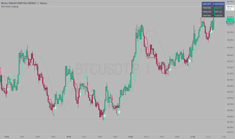
Dark VectorThe Dark Vector is a professional-grade trend-following system designed to solve the two most common causes of trading losses: over-trading during chop and exiting trends too early.
Unlike standard indicators that continuously recalculate based on every price tick, this system operates on a strict "State Machine" logic. This means it tracks the current market phase and refuses to issue conflicting signals. If the system is Long, it mathematically cannot issue another Long signal until the previous trend has concluded.
The system relies on three core engines:
1. The Trend Architecture (Modified SuperTrend) The backbone of the system is an ATR-based trailing stop mechanism. It creates a dynamic trend line that adjusts to volatility. When volatility expands, the line widens to prevent premature stop-outs during market noise. When volatility contracts, the line tightens to protect profits.
2. The Noise Gate (Choppiness Index) This is the system's safety filter. It measures the fractal efficiency of the market—essentially determining if price is moving in a clear direction or moving sideways. When the market enters a consolidation phase (sideways chop), the Noise Gate activates, turning the candles gray and physically blocking all new entry signals. This prevents the user from entering trades in low-probability environments.
3. The Singularity State Machine This internal logic enforces trading discipline. It treats the trend as a binary state (Bullish or Bearish). It forces an alternating signal pattern, ensuring that you are only alerted to the specific moment a major trend reversal occurs, rather than being bombarded with repetitive signals during a long run.
Best Way to Use This System
To maximize profitability and minimize false positives, it is recommended to use the "Regime & Alignment" methodology outlined below.
1. The Traffic Light Rule
Before placing any trade, observe the color of the candlesticks on the chart:
Green Candles: The market is in a confirmed Bullish Impulse. You should only look for Long entries or hold existing positions. Shorting is statistically dangerous here.
Red Candles: The market is in a confirmed Bearish Impulse. You should only look for Short entries or hold cash. Buying the dip here is high-risk.
Gray Candles: The market is in a Chop/Squeeze regime. The Noise Gate is active. Do not open new positions. This indicates indecision, and the market is likely to destroy option premiums or stop out tight leverage. Wait for the candles to return to Green or Red before acting.
2. The Entry Trigger
Enter a trade only when a text label (LONG or SHORT) appears.
Long Signal: Occurs when price closes above the Trend Line AND the market is not in a Chop zone.
Short Signal: Occurs when price closes below the Trend Line AND the market is not in a Chop zone.
3. The Exit Strategy
There are two ways to manage the trade once active:
The Trend Follower (Conservative): Hold the position until the Trend Line flips color. This captures the maximum duration of the move but may give back some profit at the very end.
The Stop Loss (Active): The Trend Line (the white value in your dashboard) acts as your Trailing Stop. If a candle closes beyond this line, the trend is technically invalidated. You should exit immediately.
4. Multi-Timeframe Alignment (The Golden Rule)
The highest win rates are achieved when your trading timeframe aligns with the higher-order trend.
Step 1: Check the 4-Hour chart. Is the Trend Line Green?
Step 2: Switch to the 15-Minute chart.
Step 3: Only take the LONG signals on the 15-Minute chart. Ignore all Short signals.
Reasoning: Counter-trend trades often fail. By trading only in the direction of the higher timeframe, you are swimming with the current, not against it.
Recommended Settings by Style
Swing Trading (Daily/4H): Keep the Trend Factor at 4.0. This ignores daily noise and keeps you in the trade for weeks or months.
Day Trading (1H/15m): Lower the Trend Factor to 3.0. This makes the system more reactive to intraday reversals.
Scalping (5m): Lower the Trend Factor to 2.0 and the ATR Length to 7. This is aggressive and requires strict adherence to the Stop Loss.
Disclaimer
This indicator is for educational and informational purposes only. It does not constitute financial advice, investment advice, or a recommendation to buy or sell any asset. Trading cryptocurrencies, stocks, and futures involves a high degree of risk and the potential for significant financial loss. The user assumes all responsibility for their trading decisions. Past performance of any system or indicator is not indicative of future results. Always practice risk management and never trade with money you cannot afford to lose.
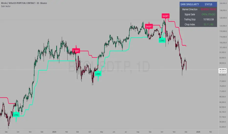
Superior-Range Bound Renko - Strategy - 11-29-25 - SignalLynxSuperior-Range Bound Renko Strategy with Advanced Risk Management Template
Signal Lynx | Free Scripts supporting Automation for the Night-Shift Nation 🌙
1. Overview
Welcome to Superior-Range Bound Renko (RBR) — a volatility-aware, structure-respecting swing-trading system built on top of a full Risk Management (RM) Template from Signal Lynx.
Instead of relying on static lookbacks (like “14-period RSI”) or plain MA crosses, Superior RBR:
Adapts its range definition to market volatility in real time
Emulates Renko Bricks on a standard, time-based chart (no Renko chart type required)
Uses a stack of Laguerre Filters to detect genuine impulse vs. noise
Adds an Adaptive SuperTrend powered by a small k-means-style clustering routine on volatility
Under the hood, this script also includes the full Signal Lynx Risk Management Engine:
A state machine that separates “Signal” from “Execution”
Layered exit tools: Stop Loss, Trailing Stop, Staged Take Profit, Advanced Adaptive Trailing Stop (AATS), and an RSI-style stop (RSIS)
Designed for non-repainting behavior on closed candles by basing execution-critical logic on previous-bar data
We are publishing this as an open-source template so traders and developers can leverage a professional-grade RM engine while integrating their own signal logic if they wish.
2. Quick Action Guide (TL;DR)
Best Timeframe:
4 Hours (H4) and above. This is a high-conviction swing-trading system, not a scalper.
Best Assets:
Volatile instruments that still respect market structure:
Bitcoin, Ethereum, Gold (XAUUSD), high-volatility Forex pairs (e.g., GBPJPY), indices with clean ranges.
Strategy Type:
Volatility-Adaptive Trend Following + Impulse Detection.
It hunts for genuine expansion out of ranges, not tiny mean-reversion nibbles.
Key Feature:
Renko Emulation on time-based candles.
We mathematically model Renko Bricks and overlay them on your standard chart to define:
“Equilibrium” zones (inside the brick structure)
“Breakout / impulse” zones (when price AND the impulse line depart from the bricks)
Repainting:
Designed to be non-repainting on closed candles.
All RM execution logic uses confirmed historical data (no future bars, no security() lookahead). Intrabar flicker during formation is allowed, but once a bar closes the engine’s decisions are stable.
Core Toggles & Filters:
Enable Longs and Shorts independently
Optional Weekend filter (block trades on Saturday/Sunday)
Per-module toggles: Stop Loss, Trailing Stop, Staged Take Profits, AATS, RSIS
3. Detailed Report: How It Works
A. The Strategy Logic: Superior RBR
Superior RBR builds its entry signal from multiple mathematical layers working together.
1) Adaptive Lookback (Volatility Normalization)
Instead of a fixed 100-bar or 200-bar range, the script:
Computes ATR-based volatility over a user-defined period.
Normalizes that volatility relative to its recent min/max.
Maps the normalized value into a dynamic lookback window between a minimum and maximum (e.g., 4 to 100 bars).
High Volatility:
The lookback shrinks, so the system reacts faster to explosive moves.
Low Volatility:
The lookback expands, so the system sees a “bigger picture” and filters out chop.
All the core “Range High/Low” and “Range Close High/Low” boundaries are built on top of this adaptive window.
2) Range Construction & Quick Ranges
The engine constructs several nested ranges:
Outer Range:
rangeHighFinal – dynamic highest high
rangeLowFinal – dynamic lowest low
Inner Close Range:
rangeCloseHighFinal – highest close
rangeCloseLowFinal – lowest close
Quick Ranges:
“Half-length” variants of those, used to detect more responsive changes in structure and volatility.
These ranges define:
The macro box price is trading inside
Shorter-term “pressure zones” where price is coiling before expansion
3) Renko Emulation (The Bricks)
Rather than using the Renko chart type (which discards time), this script emulates Renko behavior on your normal candles:
A “brick size” is defined either:
As a standard percentage move, or
As a volatility-driven (ATR) brick, optionally inhibited by a minimum standard size
The engine tracks a base value and derives:
brickUpper – top of the emulated brick
brickLower – bottom of the emulated brick
When price moves sufficiently beyond those levels, the brick “shifts”, and the directional memory (renkoDir) updates:
renkoDir = +2 when bricks are advancing upward
renkoDir = -2 when bricks are stepping downward
You can think of this as a synthetic Renko tape overlaid on time-based candles:
Inside the brick: equilibrium / consolidation
Breaking away from the brick: momentum / expansion
4) Impulse Tracking with Laguerre Filters
The script uses multiple Laguerre Filters to smooth price and brick-derived data without traditional lag.
Key filters include:
LagF_1 / LagF_W: Based on brick upper/lower baselines
LagF_Q: Based on HLCC4 (high + low + 2×close)/4
LagF_Y / LagF_P: Complex averages combining brick structures and range averages
LagF_V (Primary Impulse Line):
A smooth, high-level impulse line derived from a blend of the above plus the outer ranges
Conceptually:
When the impulse line pushes away from the brick structure and continues in one direction, an impulse move is underway.
When its direction flips and begins to roll over, the impulse is fading, hinting at mean reversion back into the range.
5) Fib-Based Structure & Swaps
The system also layers in Fib levels derived from the adaptive ranges:
Standard levels (12%, 23.6%, 38.2%, 50%, 61%, 76.8%, 88%) from the main range
A secondary “swap” set derived from close-range dynamics (fib12Swap, fib23Swap, etc.)
These Fibs are used to:
Bucket price into structural zones (below 12, between 23–38, etc.)
Detect breakouts when price and Laguerre move beyond key Fib thresholds
Drive zSwap logic (where a secondary Fib set becomes the active structure once certain conditions are met)
6) Adaptive SuperTrend with K-Means-Style Volatility Clustering
Under the hood, the script uses a small k-means-style clustering routine on ATR:
ATR is measured over a fixed period
The range of ATR values is split into Low, Medium, High volatility centroids
Current ATR is assigned to the nearest centroid (cluster)
From that, a SuperTrend variant (STK) is computed with dynamic sensitivity:
In quiet markets, SuperTrend can afford to be tighter
In wild markets, it widens appropriately to avoid constant whipsaw
This SuperTrend-based oscillator (LagF_K and its signals) is then combined with the brick and Laguerre stack to confirm valid trend regimes.
7) Final Baseline Signals (+2 / -2)
The “brain” of Superior RBR lives in the Baseline & Signal Generation block:
Two composite signals are built: B1 and B2:
They combine:
Fib breakouts
Renko direction (renkoDir)
Expansion direction (expansionQuickDir)
Multiple Laguerre alignments (LagF_Q, LagF_W, LagF_Y, LagF_Z, LagF_P, LagF_V)
They also factor in whether Fib structures are expanding or contracting.
A user toggle selects the “Baseline” signal:
finalSig = B2 (default) or B1 (alternate baseline)
finalSig is then filtered through the RM state machine and only when everything aligns, we emit:
+2 = Long / Buy signal
-2 = Short / Sell signal
0 = No new trade
Those +2 / -2 values are what feed the Risk Management Engine.
B. The Risk Management (RM) Engine
This script features the Signal Lynx Risk Management Engine, a proprietary state machine built to separate Signal from Execution.
Instead of firing orders directly on indicator conditions, we:
Convert the raw signal into a clean integer (Fin = +2 / -2 / 0)
Feed it into a Trade State Machine that understands:
Are we flat?
Are we in a long or short?
Are we in a closing sequence?
Should we permit re-entry now or wait?
Logic Injection / Template Concept:
The RM engine expects a simple integer:
+2 → Buy
-2 → Sell
Everything else (0) is “no new trade”
This makes the script a template:
You can remove the Superior RBR block
Drop in your own logic (RSI, MACD, price action, etc.)
As long as you output +2 or -2 into the same signal channel, the RM engine can drive all exits and state transitions.
Aggressive vs Conservative Modes:
The input AgressiveRM (Aggressive RM) governs how we interpret signals:
Conservative Mode (Aggressive RM = false):
Uses a more filtered internal signal (AF) to open trades
Effectively waits for a clean trend flip / confirmation before new entries
Minimizes whipsaw at the cost of fewer trades
Aggressive Mode (Aggressive RM = true):
Reacts directly to the fresh alert (AO) pulses
Allows faster re-entries in the same direction after RM-based exits
Still respects your pyramiding setting; this script ships with pyramiding = 0 by default, so it will not stack multiple positions unless you change that parameter in the strategy() call.
The state machine enforces discipline on top of your signal logic, reducing double-fires and signal spam.
C. Advanced Exit Protocols (Layered Defense)
The exit side is where this template really shines. Instead of a single “take profit or stop loss,” it uses multiple, cooperating layers.
1) Hard Stop Loss
A classic percentage-based Stop Loss (SL) relative to the entry price.
Acts as a final “catastrophic protection” layer for unexpected moves.
2) Standard Trailing Stop
A percentage-based Trailing Stop (TS) that:
Activates only after price has moved a certain percentage in your favor (tsActivation)
Then trails price by a configurable percentage (ts)
This is a straightforward, battle-tested trailing mechanism.
3) Staged Take Profits (Three Levels)
The script supports three staged Take Profit levels (TP1, TP2, TP3):
Each stage has:
Activation percentage (how far price must move in your favor)
Trailing amount for that stage
Position percentage to close
Example setup:
TP1:
Activate at +10%
Trailing 5%
Close 10% of the position
TP2:
Activate at +20%
Trailing 10%
Close another 10%
TP3:
Activate at +30%
Trailing 5%
Close the remaining 80% (“runner”)
You can tailor these quantities for partial scaling out vs. letting a core position ride.
4) Advanced Adaptive Trailing Stop (AATS)
AATS is a sophisticated volatility- and structure-aware stop:
Uses Hirashima Sugita style levels (HSRS) to model “floors” and “ceilings” of price:
Dungeon → Lower floors → Mid → Upper floors → Penthouse
These levels classify where current price sits within a long-term distribution.
Combines HSRS with Bollinger-style envelopes and EMAs to determine:
Is price extended far into the upper structure?
Is it compressed near the lower ranges?
From this, it computes an adaptive factor that controls how tight or loose the trailing level (aATS / bATS) should be:
High Volatility / Penthouse areas:
Stop loosens to avoid getting wicked out by inevitable spikes.
Low Volatility / compressed structure:
Stop tightens to lock in and protect profit.
AATS is designed to be the “smart last line” that responds to context instead of a single fixed percentage.
5) RSI-Style Stop (RSIS)
On top of AATS, the script includes a RSI-like regime filter:
A McGinley Dynamic mean of price plus ATR bands creates a dynamic channel.
Crosses above the top band and below the lower band change a directional state.
When enabled (UseRSIS):
RSIS can confirm or veto AATS closes:
For longs: A shift to bearish RSIS can force exits sooner.
For shorts: A shift to bullish RSIS can do the same.
This extra layer helps avoid over-reactive stops in strong trends while still respecting a regime change when it happens.
D. Repainting Protection
Many strategies look incredible in the Strategy Tester but fail in live trading because they rely on intrabar values or future-knowledge functions.
This template is built with closed-candle realism in mind:
The Risk Management logic explicitly uses previous bar data (open , high , low , close ) for the key decisions on:
Trailing stop updates
TP triggers
SL hits
RM state transitions
No security() lookahead or future-bar access is used.
This means:
Backtest behavior is designed to match what you can actually get with TradingView alerts and live automation.
Signals may “flicker” intrabar while the candle is forming (as with any strategy), but on closed candles, the RM decisions are stable and non-repainting.
4. For Developers & Modders
We strongly encourage you to mod this script.
To plug your own strategy into the RM engine:
Look for the section titled:
// BASELINE & SIGNAL GENERATION
You will see composite logic building B1 and B2, and then selecting:
baseSig = B2
altSig = B1
finalSig = sigSwap ? baseSig : altSig
You can replace the content used to generate baseSig / altSig with your own logic, for example:
RSI crosses
MACD histogram flips
Candle pattern detectors
External condition flags
Requirements are simple:
Your final logic must output:
2 → Buy signal
-2 → Sell signal
0 → No new trade
That output flows into the RM engine via finalSig → AlertOpen → state machine → Fin.
Once you wire your signals into finalSig, the entire Risk Management system (Stops, TPs, AATS, RSIS, re-entry logic, weekend filters, long/short toggles) becomes available for your custom strategy without re-inventing the wheel.
This makes Superior RBR not just a strategy, but a reference architecture for serious Pine dev work.
5. About Signal Lynx
Automation for the Night-Shift Nation 🌙
Signal Lynx focuses on helping traders and developers bridge the gap between indicator logic and real-world automation. The same RM engine you see here powers multiple internal systems and templates, including other public scripts like the Super-AO Strategy with Advanced Risk Management.
We provide this code open source under the Mozilla Public License 2.0 (MPL-2.0) to:
Demonstrate how Adaptive Logic and structured Risk Management can outperform static, one-layer indicators
Give Pine Script users a battle-tested RM backbone they can reuse, remix, and extend
If you are looking to automate your TradingView strategies, route signals to exchanges, or simply want safer, smarter strategy structures, please keep Signal Lynx in your search.
License: Mozilla Public License 2.0 (Open Source).
If you make beneficial modifications, please consider releasing them back to the community so everyone can benefit.

Super-AO with Risk Management Alerts Template - 11-29-25Super-AO with Risk Management: ALERTS & AUTOMATION Edition
Signal Lynx | Free Scripts supporting Automation for the Night-Shift Nation 🌙
1. Overview
This is the Indicator / Alerts companion to the Super-AO Strategy.
While the Strategy version is built for backtesting (verifying profitability and checking historical performance), this Indicator version is built for Live Execution.
We understand the frustration of finding a great strategy, only to realize you can't easily hook it up to your trading bot. This script solves that. It contains the exact same "Super-AO" logic and "Risk Management Engine" as the strategy version, but it is optimized to send signals to automation platforms like Signal Lynx, 3Commas, or any Webhook listener.
2. Quick Action Guide (TL;DR)
Purpose: Live Signal Generation & Automation.
Workflow:
Use the Strategy Version to find profitable settings.
Copy those settings into this Indicator Version.
Set a TradingView Alert using the "Any Alert() function call" condition.
Best Timeframe: 4 Hours (H4) and above.
Compatibility: Works with any webhook-based automation service.
3. Why Two Scripts?
Pine Script operates in two distinct modes:
Strategy Mode: Calculates equity, drawdowns, and simulates orders. Great for research, but sometimes complex to automate.
Indicator Mode: Plots visual data on the chart. This is the preferred method for setting up robust alerts because it is lighter weight and plots specific values that automation services can read easily.
The Golden Rule: Always backtest on the Strategy, but trade on the Indicator. This ensures that what you see in your history matches what you execute in real-time.
4. How to Automate This Script
This script uses a "Visual Spike" method to trigger alerts. Instead of drawing equity curves, it plots numerical values at the bottom of your chart when a trade event occurs.
The Signal Map:
Blue Spike (2 / -2): Entry Signal (Long / Short).
Yellow Spike (1 / -1): Risk Management Close (Stop Loss / Trend Reversal).
Green Spikes (1, 2, 3): Take Profit Levels 1, 2, and 3.
Setup Instructions:
Add this indicator to your chart.
Open your TradingView "Alerts" tab.
Create a new Alert.
Condition: Select SAO - RM Alerts Template.
Trigger: Select Any Alert() function call.
Message: Paste your JSON webhook message (provided by your bot service).
5. The Logic Under the Hood
Just like the Strategy version, this indicator utilizes:
SuperTrend + Awesome Oscillator: High-probability swing trading logic.
Non-Repainting Engine: Calculates signals based on confirmed candle closes to ensure the alert you get matches the chart reality.
Advanced Adaptive Trailing Stop (AATS): Internally calculates volatility to determine when to send a "Close" signal.
6. About Signal Lynx
Automation for the Night-Shift Nation 🌙
We are providing this code open source to help traders bridge the gap between manual backtesting and live automation. This code has been in action since 2022.
If you are looking to automate your strategies, please take a look at Signal Lynx in your search.
License: Mozilla Public License 2.0 (Open Source). If you make beneficial modifications, please release them back to the community!
