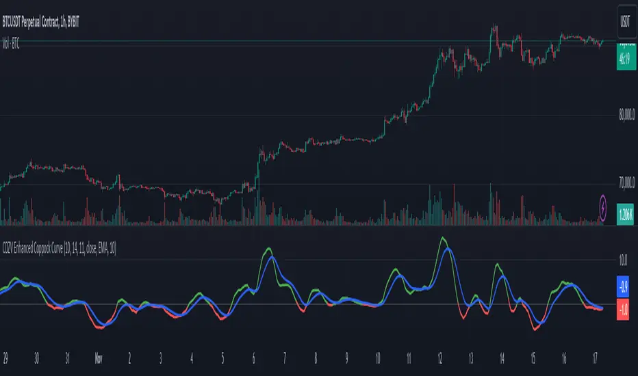
CDZV Enhanced Coppock CurveThis indicator is a part of the CDZV toolkit (backtesting and automation)
The Enhanced Coppock Curve is an upgraded version of the classic Coppock Curve indicator. It incorporates several additional features for greater flexibility and analysis capabilities. This indicator is used to analyze market trends by plotting a weighted moving average (WMA) of the sum of two Rate of Change (ROC) values.
Key Features of the Indicator:
Base Calculation of the Coppock Curve:
The Coppock Curve is calculated as a weighted moving average (WMA) of the sum of two ROC values (long and short periods).
The source for the calculation is customizable (default is close).
Added Custom Moving Average:
The indicator supports three types of moving averages:
EMA (Exponential Moving Average),
SMA (Simple Moving Average),
HMA (Hull Moving Average).
Users can choose the type and length of the moving average via input settings.
The selected moving average values are displayed in the Data Window for easier analysis.
Dynamic Coloring of the Coppock Curve:
The Coppock Curve line changes color based on its value:
Green if the value is positive,
Red if the value is negative.
The line's color is also displayed in the Data Window as a numeric value:
1 for green (positive),
-1 for red (negative).
Data Window Output:
The values of the selected moving average are displayed in the Data Window.
The Coppock Curve line's color state (1 or -1) is also shown in the Data Window.
Visual Representation:
The Coppock Curve is plotted with dynamic color coding.
The selected moving average is overlaid on the Coppock Curve for deeper trend analysis.
Usage Instructions:
Add the indicator to your chart on TradingView.
Configure the inputs:
Smoothing length for the Coppock Curve,
Long and short periods for ROC,
Type and length of the moving average.
Analyze the chart:
A green Coppock Curve line indicates a bullish trend, while a red line signals a bearish trend.
The selected moving average helps further filter and confirm signals.
Use the Data Window to view numeric values for the moving average and the Coppock Curve line color.
Applications:
This indicator is ideal for assessing trend direction and strength. The added customization options and additional data make it a versatile tool for traders, enabling them to tailor the Coppock Curve to their strategies.
在腳本中搜尋"roc"
Global Liquidity Index and DEMA1001. Global Liquidity Index:
The code calculates global liquidity from economic data from multiple countries and regions. Specifically, it aggregates money supply data from major economies such as the United States, Europe, China, and Japan, and sums and adjusts them to get a global liquidity index.
This index is calculated by summing data from different sources and subtracting the impact of some financial instruments (such as reverse repurchase agreements, etc.), and then converting the result into a number in trillions. This can help analyze the liquidity conditions in global money markets.
2. ROC SMA (Simple Moving Average of Rate of Change):
The code calculates the rate of change (ROC) of the global liquidity index, which is a way to measure the speed of change of the index.
Then, a simple moving average (SMA) is applied to the rate of change, which helps smooth the data and identify trends.
The ROC SMA curve is displayed in yellow to help users observe the trend of liquidity changes.
3. DEMA (Double Exponential Moving Average):
DEMA is a more complex moving average that attempts to reduce the lag of the moving average and provide a more sensitive trend response.
The calculation method is to first calculate a standard exponential moving average (EMA), then calculate the EMA of this EMA, and use these two results to calculate DEMA.
The code allows users to set the period length of DEMA (default is 100), which can adjust the speed of DEMA's response to price changes.
The DEMA curve is displayed in blue, helping users to more accurately capture the trends and changes of global liquidity indicators.

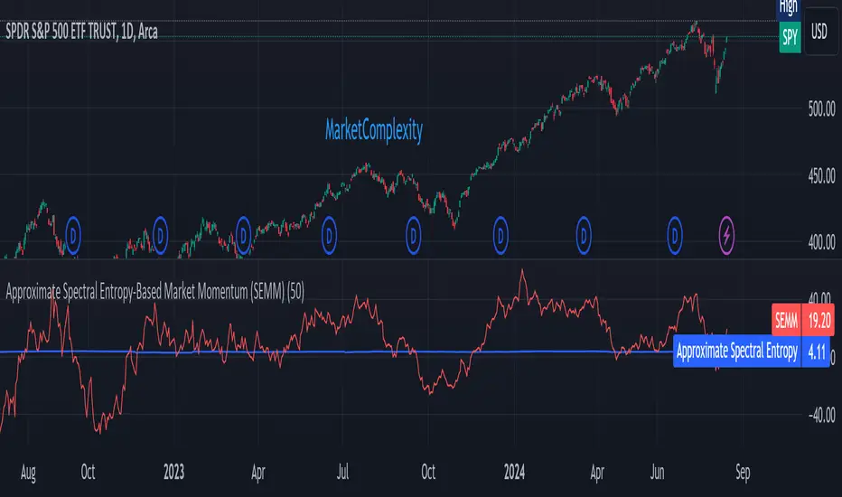
Approximate Spectral Entropy-Based Market Momentum (SEMM)Overview
The Approximate Spectral Entropy-Based Market Momentum (SEMM) indicator combines the concepts of spectral entropy and traditional momentum to provide traders with insights into both the strength and the complexity of market movements. By measuring the randomness or predictability of price changes, SEMM helps traders understand whether the market is in a trending or consolidating state and how strong that trend or consolidation might be.
Key Features
Entropy Measurement: Calculates the approximate spectral entropy of price movements to quantify market randomness.
Momentum Analysis: Integrates entropy with rate-of-change (ROC) to highlight periods of strong or weak momentum.
Dynamic Market Insight: Provides a dual perspective on market behavior—both the trend strength and the underlying complexity.
Customizable Parameters: Adjustable window length for entropy calculation, allowing for fine-tuning to suit different market conditions.
Concepts Underlying the Calculations
The indicator utilizes Shannon entropy, a concept from information theory, to approximate the spectral entropy of price returns. Spectral entropy traditionally involves a Fourier Transform to analyze the frequency components of a signal, but due to Pine Script limitations, this indicator uses a simplified approach. It calculates log returns over a rolling window, normalizes them, and then computes the Shannon entropy. This entropy value represents the level of disorder or complexity in the market, which is then multiplied by traditional momentum measures like the rate of change (ROC).
How It Works
Price Returns Calculation: The indicator first computes the log returns of price data over a specified window length.
Entropy Calculation: These log returns are normalized and used to calculate the Shannon entropy, representing market complexity.
Momentum Integration: The calculated entropy is then multiplied by the rate of change (ROC) of prices to generate the SEMM value.
Signal Generation: High SEMM values indicate strong momentum with higher randomness, while low SEMM values indicate lower momentum with more predictable trends.
How Traders Can Use It
Trend Identification: Use SEMM to identify strong trends or potential trend reversals. Low entropy values can indicate a trending market, whereas high entropy suggests choppy or consolidating conditions.
Market State Analysis: Combine SEMM with other indicators or chart patterns to confirm the market's state—whether it's trending, ranging, or transitioning between states.
Risk Management: Consider high SEMM values as a signal to be cautious, as they suggest increased market unpredictability.
Example Usage Instructions
Add the Indicator: Apply the "Approximate Spectral Entropy-Based Market Momentum (SEMM)" indicator to your chart.
Adjust Parameters: Modify the length parameter to suit your trading timeframe. Shorter lengths are more responsive, while longer lengths smooth out the signal.
Analyze the Output: Observe the blue line for entropy and the red line for SEMM. Look for divergences or confirmations with price action to guide your trades.
Combine with Other Tools: Use SEMM alongside moving averages, support/resistance levels, or other indicators to build a comprehensive trading strategy.
Average of CBO and CBO divergence histogramShort Description:
This indicator combines a Custom Bias Oscillator (CBO) with its Divergence Histogram and computes their average for use to assess the market's bias based on candlestick analysis, from the aforementioned CBO indicator.
Full Description:
Overview:
This indicator integrates two powerful analytical tools into a single script: a Custom Bias Oscillator (CBO) and its Divergence Histogram. This indicator provides traders with a comprehensive view of market bias and divergence between price movements and volume, enhanced by an optional signal line derived from the combined average of these metrics.
Key Features:
Custom Bias Oscillator (CBO):
The CBO is calculated based on the body and wick biases of candlesticks, normalized by the Average True Range (ATR) to account for market volatility.
The CBO is scaled by the divergence between the Rate of Change (ROC) of volume and the ROC of the adjusted bias, ensuring it reflects potential reversals or continuations in the market.
Divergence Histogram:
The Divergence Histogram is derived from the difference between the CBO and its signal line.
This difference is normalized and plotted to provide visual cues for potential divergences, which may indicate trend exhaustion or the beginning of a new trend.
Combined Average with Signal Line:
The indicator calculates the average of the CBO and the normalized divergence, creating a combined signal that offers a more rounded perspective on market conditions.
A signal line, generated by smoothing the combined average, is plotted to help traders identify potential buy or sell signals based on crossovers.
Customization:
The indicator includes customizable parameters for the periods of the oscillator, signal line, ATR, ROC, and the combined signal line, allowing traders to tailor the indicator to different market conditions and timeframes.
How to Use:
Buy Signal: Consider a long position when the combined average crosses above the signal line, indicating potential bullish momentum.
Sell Signal: Consider a short position when the combined average crosses below the signal line, indicating potential bearish momentum.
Divergence Analysis: Use the Divergence Histogram to identify areas where price movements may be diverging from volume, signaling potential reversals or corrections.
Disclaimer:
This indicator is designed for educational and informational purposes only. It is not financial advice. Always perform your own analysis before making any investment decisions. Past performance is not indicative of future results.

Z-score Volume by SkreepanDescription:
This indicator calculates the Z-score of the trading volume over a specified period. The Z-score is a statistical measure that describes a value's relation to the mean of a group of values. In this context, it shows how far the current volume is from the average volume in terms of standard deviations.
Inputs:
ROC Length: The period used to calculate the Rate of Change (ROC) of the source price. Default is 9.
Source: The data series to calculate the ROC. Default is the closing price.
Period: The number of bars used to calculate the moving average and standard deviation of the volume. Default is 56.
Volume Z-Score Threshold: The threshold for the Z-score above which specific conditions will trigger visual markers. Default is 3.0.
Conditions:
A visual marker (triangle) is plotted on the chart when the following conditions are met:
1. The Volume Z-Score is greater than the specified threshold.
2. The open price is greater than the close price (indicating a bearish candle).
3. The ROC is less than -2.0 (indicating a significant downward movement).
Visualizations:
Markers are plotted on the chart when the conditions are met to highlight significant volume spikes under bearish conditions with strong downward price movement.
Note:
This indicator works by detecting anomalous volumes. When such volumes occur, it is considered a good signal to buy. The indicator performs well on 3-minute and 5-minute timeframes, but if you see a signal on the hourly timeframe, it serves as good confirmation on smaller timeframes. This indicator only works for buy signals.
If this indicator has been helpful to you, please leave a comment!

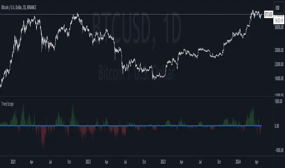
Trend ScopeIntroduction:
The Trend Scope presents a cutting-edge approach to technical analysis, offering traders a distinctive perspective on market momentum through dynamic visualization. This innovative indicator harmoniously blends the momentum-based Rate of Change (RoC) with the smoothing precision of a Butterworth filter and the clarity of a Fisher Transform, all encapsulated within an intuitive color-coded environment.
How Trend Scope Works:
The Trend Scope operates on a multi-faceted computational framework:
1. Rate of Change (RoC): The core of Trend Scope, RoC, measures the velocity of price movements, providing an initial momentum footprint that is both raw and telling.
2. Butterworth Filter: To refine the momentum signal and strip away the erratic noise of the market, we introduce the Butterworth filter. Celebrated for its flat frequency response, it ensures the retention of the signal's integrity with minimal lag.
3. Fisher Transform: To further distill the signal, the Fisher Transform is applied. It recalibrates the smoothed data to fit within specified bounds, thus accentuating the extremities of price actions where potential reversals might loom.
4. Adaptive Color Bands: The centerpiece of the Trend Scope's visual prowess lies in its adaptive color bands. These bands stretch over the momentum landscape, painted in vivid reds and greens based on the directional bias of the smoothed RoC. Intensity varies with momentum strength, offering an immediate, graphical representation of market trends.
Why Trend Scope Stands Out:
In the crowded realm of market indicators, Trend Scope distinguishes itself with its visual-forward approach and adaptive nuances. The intensity-adapting bands offer an instant read on the market's pulse—brighter shades signal stronger momentum, while muted tones suggest caution.
Key Features:
- Momentum Intensity Bands: Instead of mere lines, the Trend Scope deploys color bands that dynamically adapt in opacity to reflect the strength of the trend, making it easier for traders to spot significant movements at a glance.
- Volatility-Sensitive Smoothing: By leveraging the Butterworth filter, the Trend Scope finely tunes the noise reduction process in sync with the asset's natural volatility, ensuring the trends are not only smooth but also relevant.
- Sharper Reversal Signals: The Fisher Transform sharpens the ability to spot potential turning points, providing a statistical edge in anticipating market movements.
- Customizable Parameters: The Trend Scope is fully customizable, allowing traders to calibrate the indicator to the unique demands of different assets and market conditions.
Yeong RRGThe code outlines a trading strategy that leverages Relative Strength (RS) and Rate of Change (RoC) to make trading decisions. Here's a detailed breakdown of the tactic described by the code:
Ticker and Period Selection: The strategy begins by selecting a stock ticker symbol and defining a period (len) for the calculations, which defaults to 14 but can be adjusted by the user.
Stock and Index Data Retrieval: It fetches the closing price (stock_close) of the chosen stock and calculates its 25-period exponential moving average (stock_ema). Additionally, it retrieves the closing price of the S&P 500 Index (index_close), used as a benchmark for calculating Relative Strength.
Relative Strength Calculation: The Relative Strength (rs) is computed by dividing the stock's closing price by the index's closing price, then multiplying by 100 to scale the result. This metric is used to assess the stock's performance relative to the broader market.
Moving RS Ratio and Rate of Change: The strategy calculates a Simple Moving Average (sma) of the RS over the specified period to get the RS Ratio (rs_ratio). It then computes the Rate of Change (roc) of this RS Ratio over the same period to get the RM Ratio (rm_ratio).
Normalization: The RS Ratio and RM Ratio are normalized using a formula that adjusts their values based on the mean and standard deviation of their respective series over the specified window. This normalization process helps in standardizing the indicators, making them easier to interpret and compare.
Indicator Plotting: The normalized RS Ratio (jdk_rs_ratio) and RM Ratio (jdk_rm_ratio) are plotted on the chart with different colors for visual analysis. A horizontal line (hline) at 100 serves as a reference point, indicating a neutral level for the indicators.
State Color Logic: The script includes a logic to determine the state color (statecolor) based on the previous state color and the current values of jdk_rs_ratio and jdk_rm_ratio. This color coding is intended to visually represent different market states: green for bullish, red for bearish, yellow for hold, and blue for watch conditions.
Signal Generation: The strategy generates buy, sell, hold, and watch signals based on the state color and the indicators' values relative to 100. For example, a buy signal is generated when both jdk_rs_ratio and jdk_rm_ratio are above 100, and the background color is set to green to reflect this bullish condition.
Trade Execution: Finally, the strategy executes trades based on the generated signals. A "BUY" trade is entered when a buy signal is present, and it is closed when a sell signal occurs.
Overall, the strategy uses a combination of RS and RoC indicators, normalized for better comparison, to identify potential buy and sell opportunities based on the stock's performance relative to the market and its momentum.

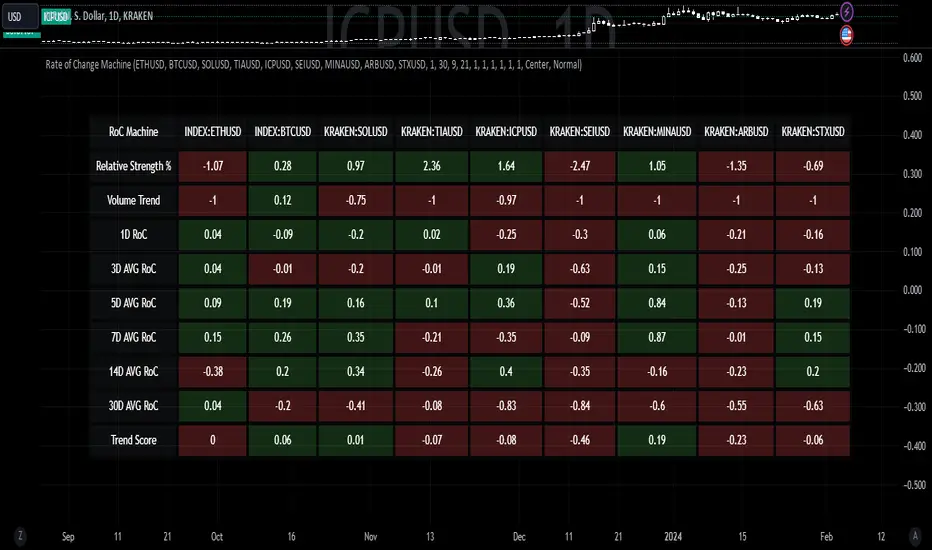
Rate of Change MachineRate of Change Machine
Author: RWCS_LTD
Disclaimer: This script is provided for informational purposes only and should not be considered financial advice. Trading involves substantial risk, and past performance is not indicative of future results. Always conduct your own research and consult with a qualified financial advisor before making any investment decisions.
Introduction:
The Rate of Change Machine is a script designed to assist traders in analyzing multiple cryptocurrency trading pairs simultaneously. This comprehensive indicator offers a holistic view of the rate of change and related metrics, aiding traders in making informed decisions.
Asset Selection:
The script enables users to select up to nine different cryptocurrency trading pairs for in-depth analysis.
Volume Calculation:
Volume plays a crucial role in the analysis, with customizable parameters for volume weighting and length.
Relative Strength Calculation:
Relative Strength is determined through two Exponential Moving Averages (EMA) with user-defined lengths.
Timeframe Weightings:
Different timeframes (1D, AVG 3D, AVG 5D, AVG 7D, AVG 14D, AVG 30D) are assigned weightings to calculate a comprehensive trend score.
Weighted Average and Individual Rate of Change (RoC) Calculation:
The getWeightedAvgAndIndividualROC function calculates the RoC for each selected trading pair based on the given timeframes and weights.
Table Setup:
A table is created to display the results for each trading pair, including relative strength, volume trend, RoC for different timeframes, and a weighted trend score.
Table Formatting:
The table is formatted with different colors indicating positive or negative values for easier interpretation.
Table Position and Size:
Users can customize the position and size of the table on the chart.
Data Retrieval:
The script retrieves the calculated values for each trading pair using the request.security function.
Output:
The final output is a table on the chart, showing relevant information for the selected trading pairs, aiding traders in making informed decisions based on the rate of change and other factors. This indicator provides a comprehensive view of the rate of change and related metrics for multiple trading pairs, assisting traders in identifying potential trends and making informed trading decisions.
VIX Statistical Sentiment Index [Nasan]** THIS IS ONLY FOR US STOCK MARKET**
The indicator analyzes market sentiment by computing the Rate of Change (ROC) for the VIX and S&P 500, visualizing the data as histograms with conditional coloring. It measures the correlation between the VIX, the specific stock, and the S&P 500, displaying the results on the chart. The reliability measure combines these correlations, offering an overall assessment of data robustness. One can use this information to gauge the inverse relationship between VIX and S&P 500, the alignment of the specific stock with the market, and the overall reliability of the correlations for informed decision-making based on the inverse relationship of VIX and price movement.
**WHEN THE VIX ROC IS ABOVE ZERO (RED COLOR) AND RASING ONE CAN EXPECT THE PRICE TO MOVE DOWNWARDS, WHEN THE VIX ROC IS BELOW ZERO (GREEN)AND DECREASING ONE CAN EXPECT THE PRICE TO MOVE UPWARDS"
Understanding the VIX Concept:
The VIX, or Volatility Index, is a widely used indicator in finance that measures the market's expectation of volatility over the next 30 days. Here are key points about the VIX:
Fear Gauge:
Often referred to as the "fear gauge," the VIX tends to rise during periods of market uncertainty or fear and fall during calmer market conditions.
Inverse Relationship with Market:
The VIX typically has an inverse relationship with the stock market. When the stock market experiences a sell-off, the VIX tends to rise, indicating increased expected volatility.
Implied Volatility:
The VIX is derived from the prices of options on the S&P 500. It represents the market's expectations for future volatility and is often referred to as "implied volatility."
Contrarian Indicator:
Extremely high VIX levels may indicate oversold conditions, suggesting a potential market rebound. Conversely, very low VIX levels may signal complacency and a potential reversal.
VIX vs. SPX Correlation:
This correlation measures the strength and direction of the relationship between the VIX (Volatility Index) and the S&P 500 (SPX).
A negative correlation indicates an inverse relationship. When the VIX goes up, the SPX tends to go down, and vice versa.
The correlation value closer to -1 suggests a stronger inverse relationship between VIX and SPX.
Stock vs. SPX Correlation:
This correlation measures the strength and direction of the relationship between the closing price of the stock (retrieved using src1) and the S&P 500 (SPX).
This correlation helps assess how closely the stock's price movements align with the broader market represented by the S&P 500.
A positive correlation suggests that the stock tends to move in the same direction as the S&P 500, while a negative correlation indicates an opposite movement.
Reliability Measure:
Combines the squared values of the VIX vs. SPX and Stock vs. SPX correlations and takes the square root to create a reliability measure.
This measure provides an overall assessment of how reliable the correlation information is in guiding decision-making.
Interpretation:
A higher reliability measure implies that the correlations between VIX and SPX, as well as between the stock and SPX, are more robust and consistent.
One can use this reliability measure to gauge the confidence they can place in the correlations when making decisions about the specific stock based on VIX data and its correlation with the broader market.

Trend Reversal Probability CalculatorThe "Trend Reversal Probability Calculator" is a TradingView indicator that calculates the probability of a trend reversal based on the crossover of multiple moving averages and the rate of change (ROC) of their slopes. This indicator is designed to help traders identify potential trend reversals by providing signals when the short-term moving averages start to slope in the opposite direction of the long-term moving average.
To use the indicator, simply add it to your TradingView chart and adjust the input parameters according to your preferences. The input parameters include the length of the moving averages, the ROC length (trend sensitivity), and the reversal sensitivity (signal percentage).
The indicator calculates the ROC of the moving averages and determines if the short-term moving averages are sloping in the opposite direction of the long-term moving average. The number of short-term moving averages that meet this condition is then counted, and the probability of a trend reversal is calculated based on the percentage of short-term moving averages that meet this condition.
When the probability of a trend reversal is high, a bullish or bearish signal is generated, depending on the direction of the reversal. The bullish signal is generated when the short-term moving averages start to slope upward, and the bearish signal is generated when the short-term moving averages start to slope downward.
Traders can use the "Trend Reversal Probability Calculator" to identify potential trend reversals and adjust their trading strategies accordingly. It is important to note that this indicator is not a guarantee of a trend reversal and should be used in conjunction with other technical analysis tools to make informed trading decisions.

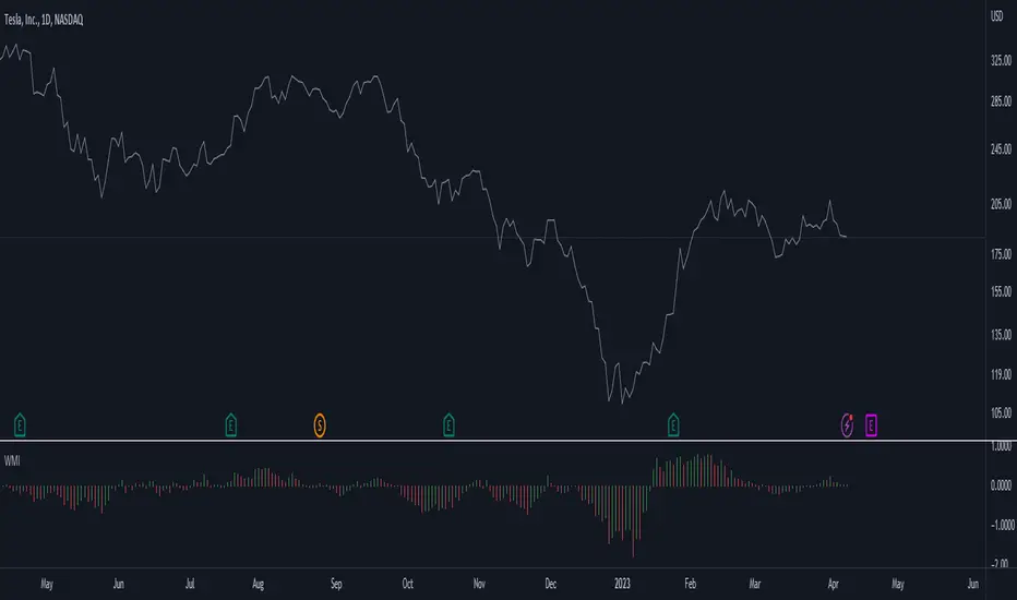
Weighted Momentum and Volatility Indicator (WMI)The Weighted Momentum and Volatility Indicator (WMI) is a composite technical analysis tool that combines momentum and volatility to identify potential trend changes in the underlying asset.
The WMI is displayed as an histogram that oscillates around a zero line, with increasing bars indicating a bullish trend and decreasing bars indicating a bearish trend.
The WMI is calculated by combining the Rate of Change (ROC) and Average True Range (ATR) indicators.
The ROC measures the percentage change in price over a set period of time, while the ATR measures the volatility of the asset over the same period.
The WMI is calculated by multiplying the normalized values of the ROC and ATR indicators, with the normalization process being used to adjust the values to a scale between 0 and 1.
Traders and investors can use the WMI to identify potential trend changes in the underlying asset, with increasing bars indicating a bullish trend and decreasing bars indicating a bearish trend.
The WMI can be used in conjunction with other technical analysis tools to develop a comprehensive trading strategy.
Do not hesitate to let me know your comments if you see any improvements to be made :)
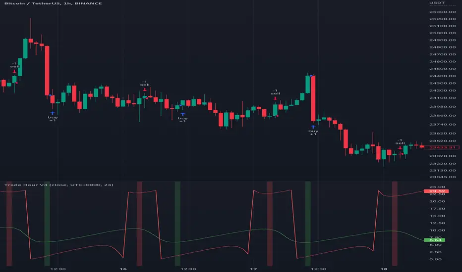
Trade HourThis script is just finds the best hour to buy and sell hour in a day by checking chart movements in past
For example if the red line is on the 0.63 on BTC/USDT chart it mean the start of 12AM hour on a day is the best hour to buy (all based on
It's just for 1 hour time-frame but you can test it on other charts.
IMPORTANT: You can change time Zone in strategy settings.to get the real hours as your location timezone
IMPORTANT: Its for now just for BTC/USDT but you can optimize and test for other charts...
IMPORTANT: A green and red background color calculated for show the user the best places of buy and sell (green : positive signal, red: negative signals)
settings :
timezone : We choice a time frame for our indicator as our geo location
source : A source to calculate rate of change for it
Time Period : Time period of ROC indicator
About Calculations:
1- We first get a plot that just showing the present hour as a zigzag plot
2- So we use an indicator ( Rate of change ) to calculate chart movements as positive and negative numbers. I tested ROC is the best indicator but you can test close-open or real indicator or etc as indicator.
3 - for observe effects of all previous data we should indicator_cum that just a full sum of indicator values.
4- now we need to split this effects to hours and find out which hour is the best place to buy and which is the best for sell. Ok we should just calculate multiple of hour*indicator and get complete sum of it so:
5- we will divide this number to indicator_cum : (indicator_mul_hour_cum) / indicator_cum
6- Now we have the best hour to buy! and for best sell we should just reverse the ROC indicator and recalculate the best hour for it!
7- A green and red background color calculated for show the user the best places of buy and sell that dynamically changing with observing green and red plots(green : positive signal, red: negative signals) when green plot on 15 so each day on hour 15 the background of strategy indicator will change to 15 and if its go upper after some days and reached to 16 the background green color will move to 16 dynamically.
Rate Of Change and rsi zonesHi,
I played with the ROC ( Rate of change ) indicator.
First of all I made it smooth. And came up with decent buy sell signals for long-term potential trades. It can be useful for DCA and profit booking in market tops ( before potential crash)
Recommended time frame = 1 Daily , 3 Daily , Weekly.
Usage :
1. Look for Buy and sell arrow signals. But don't jump straight away. Specially for sell. You might sell early. Instead you can move up your stop loss when you see a sell signal or profit book partially.
if you wait and combine with your own supply and demand zones you can get some nice sell price.
2. Better to wait and look for a divergence in price and ROC. As price will slow down it will reflect on the ROC line. Which means market is exhausted and potentially a correction might happen.
3. You can draw trendline one the ROC and look for breakout. ( warning won't always work )
4. You can also see the RSI in thick red/green color. It will help you determine oversold and overbought zones. Trick is don't sell when it's oversold ( red thick line) . Because it might be a start of a strong uptrend.
So better is to wait and see when the signal is printing then execute.
Best strategy is to DCA and sell in parts whenever you see such signals.
I believe it will visually help us that when to be bull and when to be bear.
Anyway if you find it useful let me know in the comment.
Also if you have some idea to improve the code you can contribute as well.
Thanks . Feedbacks are welcome.

pandas_taLibrary "pandas_ta"
Level: 3
Background
Today is the first day of 2022 and happy new year every tradingviewers! May health and wealth go along with you all the time. I use this chance to publish my 1st PINE v5 lib : pandas_ta
This is not a piece of cake like thing, which cost me a lot of time and efforts to build this lib. Beyond 300 versions of this script was iterated in draft.
Function
Library "pandas_ta"
PINE v5 Counterpart of Pandas TA - A Technical Analysis Library in Python 3 at github.com
The Original Pandas Technical Analysis (Pandas TA) is an easy to use library that leverages the Pandas package with more than 130 Indicators and Utility functions and more than 60 TA Lib Candlestick Patterns.
I realized most of indicators except Candlestick Patterns because tradingview built-in Candlestick Patterns are even more powerful!
I use this to verify pandas_ta python version indicators for myself, but I realize that maybe many may need similar lib for pine v5 as well.
Function Brief Descriptions (Pls find details in script comments)
bton --> Binary to number
wcp --> Weighted Closing Price (WCP)
counter --> Condition counter
xbt --> Between
ebsw --> Even Better SineWave (EBSW)
ao --> Awesome Oscillator (AO)
apo --> Absolute Price Oscillator (APO)
xrf --> Dynamic shifted values
bias --> Bias (BIAS)
bop --> Balance of Power (BOP)
brar --> BRAR (BRAR)
cci --> Commodity Channel Index (CCI)
cfo --> Chande Forcast Oscillator (CFO)
cg --> Center of Gravity (CG)
cmo --> Chande Momentum Oscillator (CMO)
coppock --> Coppock Curve (COPC)
cti --> Correlation Trend Indicator (CTI)
dmi --> Directional Movement Index(DMI)
er --> Efficiency Ratio (ER)
eri --> Elder Ray Index (ERI)
fisher --> Fisher Transform (FISHT)
inertia --> Inertia (INERTIA)
kdj --> KDJ (KDJ)
kst --> 'Know Sure Thing' (KST)
macd --> Moving Average Convergence Divergence (MACD)
mom --> Momentum (MOM)
pgo --> Pretty Good Oscillator (PGO)
ppo --> Percentage Price Oscillator (PPO)
psl --> Psychological Line (PSL)
pvo --> Percentage Volume Oscillator (PVO)
qqe --> Quantitative Qualitative Estimation (QQE)
roc --> Rate of Change (ROC)
rsi --> Relative Strength Index (RSI)
rsx --> Relative Strength Xtra (rsx)
rvgi --> Relative Vigor Index (RVGI)
slope --> Slope
smi --> SMI Ergodic Indicator (SMI)
sqz* --> Squeeze (SQZ) * NOTE: code sufferred from very strange error, code was commented.
sqz_pro --> Squeeze PRO(SQZPRO)
xfl --> Condition filter
stc --> Schaff Trend Cycle (STC)
stoch --> Stochastic (STOCH)
stochrsi --> Stochastic RSI (STOCH RSI)
trix --> Trix (TRIX)
tsi --> True Strength Index (TSI)
uo --> Ultimate Oscillator (UO)
willr --> William's Percent R (WILLR)
alma --> Arnaud Legoux Moving Average (ALMA)
xll --> Dynamic rolling lowest values
dema --> Double Exponential Moving Average (DEMA)
ema --> Exponential Moving Average (EMA)
fwma --> Fibonacci's Weighted Moving Average (FWMA)
hilo --> Gann HiLo Activator(HiLo)
hma --> Hull Moving Average (HMA)
hwma --> HWMA (Holt-Winter Moving Average)
ichimoku --> Ichimoku Kinkō Hyō (ichimoku)
jma --> Jurik Moving Average Average (JMA)
kama --> Kaufman's Adaptive Moving Average (KAMA)
linreg --> Linear Regression Moving Average (linreg)
mgcd --> McGinley Dynamic Indicator
rma --> wildeR's Moving Average (RMA)
sinwma --> Sine Weighted Moving Average (SWMA)
ssf --> Ehler's Super Smoother Filter (SSF) © 2013
supertrend --> Supertrend (supertrend)
xsa --> X simple moving average
swma --> Symmetric Weighted Moving Average (SWMA)
t3 --> Tim Tillson's T3 Moving Average (T3)
tema --> Triple Exponential Moving Average (TEMA)
trima --> Triangular Moving Average (TRIMA)
vidya --> Variable Index Dynamic Average (VIDYA)
vwap --> Volume Weighted Average Price (VWAP)
vwma --> Volume Weighted Moving Average (VWMA)
wma --> Weighted Moving Average (WMA)
zlma --> Zero Lag Moving Average (ZLMA)
entropy --> Entropy (ENTP)
kurtosis --> Rolling Kurtosis
skew --> Rolling Skew
xev --> Condition all
zscore --> Rolling Z Score
adx --> Average Directional Movement (ADX)
aroon --> Aroon & Aroon Oscillator (AROON)
chop --> Choppiness Index (CHOP)
xex --> Condition any
cksp --> Chande Kroll Stop (CKSP)
dpo --> Detrend Price Oscillator (DPO)
long_run --> Long Run
psar --> Parabolic Stop and Reverse (psar)
short_run --> Short Run
vhf --> Vertical Horizontal Filter (VHF)
vortex --> Vortex
accbands --> Acceleration Bands (ACCBANDS)
atr --> Average True Range (ATR)
bbands --> Bollinger Bands (BBANDS)
donchian --> Donchian Channels (DC)
kc --> Keltner Channels (KC)
massi --> Mass Index (MASSI)
natr --> Normalized Average True Range (NATR)
pdist --> Price Distance (PDIST)
rvi --> Relative Volatility Index (RVI)
thermo --> Elders Thermometer (THERMO)
ui --> Ulcer Index (UI)
ad --> Accumulation/Distribution (AD)
cmf --> Chaikin Money Flow (CMF)
efi --> Elder's Force Index (EFI)
ecm --> Ease of Movement (EOM)
kvo --> Klinger Volume Oscillator (KVO)
mfi --> Money Flow Index (MFI)
nvi --> Negative Volume Index (NVI)
obv --> On Balance Volume (OBV)
pvi --> Positive Volume Index (PVI)
dvdi --> Dual Volume Divergence Index (DVDI)
xhh --> Dynamic rolling highest values
pvt --> Price-Volume Trend (PVT)
Remarks
I also incorporated func descriptions and func test script in commented mode, you can test the functino with the embedded test script and modify them as you wish.
This is a Level 3 free and open source indicator library.
Feedbacks are appreciated.
This is not the end of pandas_ta lib publication, but it is start point with pine v5 lib function and I will add more and more funcs into this lib for my own indicators.
Function Name List:
bton()
wcp()
count()
xbt()
ebsw()
ao()
apo()
xrf()
bias()
bop()
brar()
cci()
cfo()
cg()
cmo()
coppock()
cti()
dmi()
er()
eri()
fisher()
inertia()
kdj()
kst()
macd()
mom()
pgo()
ppo()
psl()
pvo()
qqe()
roc()
rsi()
rsx()
rvgi()
slope()
smi()
sqz_pro()
xfl()
stc()
stoch()
stochrsi()
trix()
tsi()
uo()
willr()
alma()
wcx()
xll()
dema()
ema()
fwma()
hilo()
hma()
hwma()
ichimoku()
jma()
kama()
linreg()
mgcd()
rma()
sinwma()
ssf()
supertrend()
xsa()
swma()
t3()
tema()
trima()
vidya()
vwap()
vwma()
wma()
zlma()
entropy()
kurtosis()
skew()
xev()
zscore()
adx()
aroon()
chop()
xex()
cksp()
dpo()
long_run()
psar()
short_run()
vhf()
vortex()
accbands()
atr()
bbands()
donchian()
kc()
massi()
natr()
pdist()
rvi()
thermo()
ui()
ad()
cmf()
efi()
ecm()
kvo()
mfi()
nvi()
obv()
pvi()
dvdi()
xhh()
pvt()

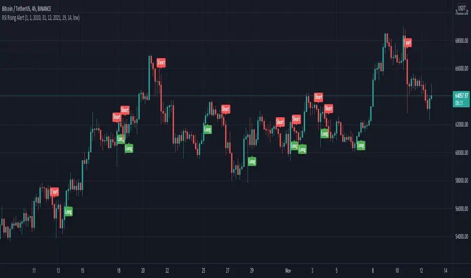
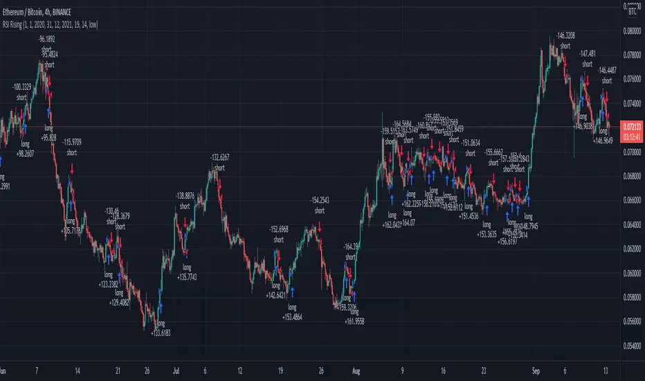
RSI Rising Crypto Trending AlertAlert version of the strategy with the same name
This is crypto and stock market trending strategy designed for long timeframes such as 4h+
From my tests it looks like it works better to trade crypto against crypto than trading against fiat.
Indicators used:
RSI for rising/falling of the trend
BB sidemarket
ROC sidemarket
Rules for entry
For long: RSI values are rising, and bb and roc tells us we are not in a sidemarket
For long: RSI values are falling, and bb and roc tells us we are not in a sidemarket
Rules for exit
We exit when we receive an opposite direction.
Cuation: Because this strategy uses no risk management, I recommend you takje care with it.
If you have any questions, let me know !
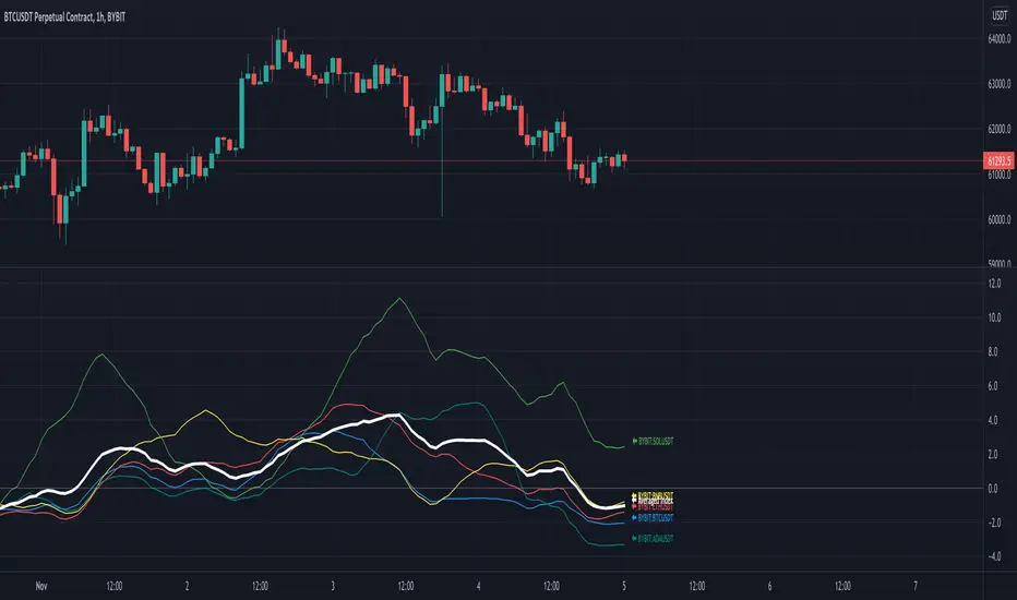
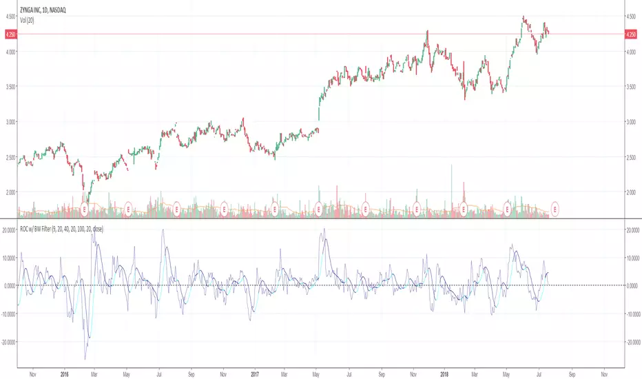
SROC Crypto Index [upslidedown]The idea for this indicator is simple: Without a crypto index we want to somehow understand ROC across many assets. This will average out data across the top 5 (current) cryptos and provide a benchmark index.
I've recently been looking into momentum strategies more and how to utilize ROC as part of crypto trading. This indicator was born to fill a void as there is no great index like SPY for the crypto world.
Why would you do this? This gives a picture of overall market sentiment and allows you to move stock strategies that use an index to do things like tighten SL, take positions, move to cash, etc. into the cryptocurrency market.
The plotted line is super fat so you can plot individual lines and tell the index from the individual ticker apart. My suggestion is to pair this with a ROC or SROC for individual assets and to develop strategies from there.
RSI Rising Crypto Trending StrategyThis is crypto and stock market trending strategy designed for long timeframes such as 4h+
From my tests it looks like it works better to trade crypto against crypto than trading against fiat.
Indicators used:
RSI for rising/falling of the trend
BB sidemarket
ROC sidemarket
Rules for entry
For long: RSI values are rising, and bb and roc tells us we are not in a sidemarket
For long: RSI values are falling, and bb and roc tells us we are not in a sidemarket
Rules for exit
We exit when we receive an opposite direction.
Cuation: Because this strategy uses no risk management, I recommend you takje care with it.
If you have any questions, let me know !
Volatility ArbitrageDescription:
This indicator uses rate of change (ROC) indicator and its standard deviations.
ROC values are cycling around zero, i.e. around the mean.
Two standard deviations of the ROC draw the upper and the lower bounds that serve as thresholds.
These capture outliers that can be used as signals.

Rate of Change w/ Butterworth FilterIt passes the Rate of Change data through a Butterworth filter which creates a smooth line that can allow for easier detection of slope changes in the data over various periods of times.
The butterworth filter line and the rate of change are plotted together by default. The values for the lengths, for both the butterworth filter and the raw ROC data, can be changed from the format menu (through a toggle).
The shorter the Butterworth length, the closer the line is fitted to the raw ROC data, however you trade of with more frequent slope changes.
The longer the Butterworth length, the smoother the line and less frequent the slope changes, but the Butterworth line is farther of center from the raw ROC data.
Momentum Color Classification System### Code Analysis: Momentum Color Classification System (Pine Script v5)
#### Core Function
This is a **non-overlay TradingView Pine Script v5 indicator** designed to quantify and categorize price momentum dynamics with extreme precision. It calculates core momentum from price Rate of Change (ROC) and second-derivative momentum change, then classifies market momentum into 9 distinct states (bullish variations, bearish variations, and neutral oscillation). The indicator visualizes momentum via color-coded histogram bars, and provides real-time status labels, a detailed info dashboard, and actionable trading suggestions — all to help traders accurately identify momentum strength, acceleration/deceleration trends, and guide long/short trading decisions.
#### Key Features (Concise & Clear)
1. **9-tier Precise Momentum Classification**
Divides momentum into **4 bullish states** (accelerating/decelerating/steady/weak up), **4 bearish states** (accelerating/decelerating/steady/weak down) and 1 neutral oscillation state, fully covering all momentum trend phases in the market.
2. **2-dimensional Momentum Calculation**
Combines **1st-order momentum** (price ROC-based core momentum) and **2nd-order momentum change** (momentum acceleration/deceleration), plus absolute momentum strength, to comprehensively judge momentum direction, speed and intensity.
3. **Color-Coded Visualization with Hierarchy**
Uses a gradient color system (vibrant-to-pale green for bullish, vivid-to-light red for bearish, gray for neutral) with transparency differentiation to reflect momentum strength; histogram style ensures intuitive observation, paired with a dotted zero reference line for clear bias judgment.
4. **Practical Trading Auxiliary Tools**
Supports toggleable status labels for extreme momentum (accelerating up/down); embeds a top-right dashboard displaying real-time momentum values, change rate, state, strength level and direct trading suggestions, enabling one-glance market judgment.
5. **High Customizability**
Allows adjustment of core parameters (momentum calculation period, smoothing factor) and toggling of label display, with reasonable parameter ranges to adapt to different trading assets and timeframes.
6. **Trade-Oriented Decision Guidance**
Maps each momentum state to corresponding strength levels and actionable operation advice (long/add position, short/add position, hold, reduce position, wait), directly linking technical analysis to actual trading behavior.

Velocity Divergence Radar [JOAT]
Velocity Divergence Radar - Momentum Physics Edition
Overview
Velocity Divergence Radar is an open-source oscillator indicator that applies physics concepts to market analysis. It calculates price velocity (rate of change), acceleration (rate of velocity change), and jerk (rate of acceleration change) to provide a multi-dimensional view of momentum. The indicator also includes divergence detection and force vector analysis.
What This Indicator Does
The indicator calculates and displays:
Velocity - Rate of price change over a configurable period, smoothed with EMA
Acceleration - Rate of velocity change, showing momentum shifts
Jerk (3rd Derivative) - Rate of acceleration change, indicating momentum stability
Force Vectors - Volume-weighted acceleration representing market force
Kinetic Energy - Calculated as 0.5 * mass (volume ratio) * velocity squared
Momentum Conservation - Tracks momentum relative to historical average
Divergence Detection - Identifies when price and velocity diverge at pivots
How It Works
Velocity is calculated as smoothed rate of change:
calculateVelocity(series float price, simple int period) =>
float roc = ta.roc(price, period)
float velocity = ta.ema(roc, period / 2)
velocity
Acceleration is the change in velocity:
calculateAcceleration(series float velocity, simple int period) =>
float accel = ta.change(velocity, period)
float smoothAccel = ta.ema(accel, period / 2)
smoothAccel
Jerk is the change in acceleration:
calculateJerk(series float acceleration, simple int period) =>
float jerk = ta.change(acceleration, period)
float smoothJerk = ta.ema(jerk, period / 2)
smoothJerk
Force is calculated using F = m * a (mass approximated by volume ratio):
calculateForceVector(series float mass, series float acceleration) =>
float force = mass * acceleration
float forceDirection = math.sign(force)
float forceMagnitude = math.abs(force)
Signal Generation
Signals are generated based on velocity behavior:
Bullish Divergence: Price makes lower low while velocity makes higher low
Bearish Divergence: Price makes higher high while velocity makes lower high
Velocity Cross: Velocity crosses above/below zero line
Extreme Velocity: Velocity exceeds 1.5x the upper/lower zone threshold
Jerk Extreme: Jerk exceeds 2x standard deviation
Force Extreme: Force magnitude exceeds 2x average
Dashboard Panel (Top-Right)
Velocity - Current velocity value
Acceleration - Current acceleration value
Momentum Strength - Combined velocity and acceleration strength
Radar Score - Composite score based on velocity and acceleration
Direction - STRONG UP/SLOWING UP/STRONG DOWN/SLOWING DOWN/FLAT
Jerk - Current jerk value
Force Vector - Current force magnitude
Kinetic Energy - Current kinetic energy value
Physics Score - Overall physics-based momentum score
Signal - Current actionable status
Visual Elements
Velocity Line - Main oscillator line with color based on direction
Velocity EMA - Smoothed velocity for trend reference
Acceleration Histogram - Bar chart showing acceleration direction
Jerk Area - Filled area showing jerk magnitude
Vector Magnitude - Line showing combined vector strength
Radar Scan - Oscillating pattern for visual effect
Zone Lines - Upper and lower threshold lines
Divergence Labels - BULL DIV / BEAR DIV markers
Extreme Markers - Triangles at velocity extremes
Input Parameters
Velocity Period (default: 14) - Period for velocity calculation
Acceleration Period (default: 7) - Period for acceleration calculation
Divergence Lookback (default: 10) - Bars to scan for divergence
Radar Sensitivity (default: 1.0) - Zone threshold multiplier
Jerk Analysis (default: true) - Enable 3rd derivative calculation
Force Vectors (default: true) - Enable force analysis
Kinetic Energy (default: true) - Enable energy calculation
Momentum Conservation (default: true) - Enable momentum tracking
Suggested Use Cases
Identify momentum direction using velocity sign and magnitude
Watch for divergences as potential reversal warnings
Use acceleration to detect momentum shifts before price confirms
Monitor jerk for momentum stability assessment
Combine force and kinetic energy for conviction analysis
Timeframe Recommendations
Works on all timeframes. Higher timeframes provide smoother readings; lower timeframes show more granular momentum changes.
Limitations
Physics analogies are conceptual and not literal market physics
Divergence detection uses pivot-based lookback and may lag
Force calculation uses volume ratio as mass proxy
Kinetic energy is a derived metric, not actual energy
Open-Source and Disclaimer
This script is published as open-source under the Mozilla Public License 2.0 for educational purposes. It does not constitute financial advice. Past performance does not guarantee future results. Always use proper risk management.
- Made with passion by officialjackofalltrades

Confluence Execution Engine (2of3)The Confluence Execution Engine is a high-performance logic gate designed to filter out market noise and identify high-probability "Golden" entries. It moves beyond simple indicator signals by acting as a mathematical validator for price action. This engine is designed for the Systematic Trader. It removes the "guesswork" of whether a move is real or an exhaustion pump by requiring a mathematical confluence of volume, multi-timeframe momentum, and volatility-adjusted space.
Why This Tool is Unique:
Multi-Dimensional Scoring, Momentum-Adjusted Stretch, Institutional Fingerprint (RVOL + Spike)
Unlike a standard MACD or RSI, this engine uses a weighted scoring matrix. It pulls a "Bundle" of data (WaveTrend, RSI, ROC) from four different timeframes simultaneously. It doesn't give a signal unless the mathematical weight of all four timeframes crosses your "Hurdle" (Base Threshold).
Standard "overbought" indicators are often wrong during strong trends. This engine uses Dynamic Z-Score logic. The Logic: If the price moves away from the mean, it checks the Rate of Change (ROC). The Result: If momentum is massive, the "Stretch" limit expands. It understands that a "stretched" price is actually a sign of strength in a breakout, not a reason to exit. It only warns of a TRAP RISK when the price is far from the mean but momentum is starting to stall.
The engine is gated by Relative Volume. If the market is "sleepy," the engine stays in "PATIENCE" mode. It specifically hunts for Volume Spikes (default 2.5x average). A signal is only upgraded to "HIGH CONVICTION" when an institutional volume spike occurs, confirming that "Big Money" is participating.
How to Operate the Engine
Define Your Hurdle: Set your Confluence Hurdle. A higher number (e.g., 14+) requires more agreement across timeframes, leading to fewer but higher-quality trades.
Monitor the Z/Dynamic Ratio: In the HUD, watch the Z: X.XX / Y.YY. When X approaches Y, you are reaching the edge of the momentum-adjusted move.
The Entry Trigger: Wait for a "LOOK FOR..." advice to turn into a "HIGH CONVICTION" signal (marked by a triangle shape). This confirms that the MTF scoring, Volume, and HTF Trend are all aligned.
Execute the Lines: Use the red and green "Ghost Lines" to set your orders. These are ATR-based, meaning they widen during high volatility to give your trade room to breathe.
For holistic trading system, pair with Volatility Shield Pro and Session Levels

Long-term KST (Know Sure Thing)Description
Long-term Know Sure Thing (KST) oscillator, specifically adapted for non-24h markets such as stocks, indices, ETFs and futures.
This version correctly scales the weekly ROC periods based on the actual trading week length and daily session duration of the instrument — making it accurate across different asset classes (European indices, US equities, crypto, etc.).
Key features:
• Fully customizable trading week (5 days for most stock markets, 7 days for crypto/24h markets)
• Customizable daily session length (8.5h for FTSE MIB/DAX, 6.5h for US equities, 24h for crypto/forex)
• Automatically adjusts bar count per week on any chart timeframe (including Weekly)
• Classic Martin Pring KST parameters (10/13/15/20 ROC weeks, 10/13/15/20 SMA weeks, 1-2-3-4 weighting)
• Includes signal line (SMA of KST) and visual fill between KST and signal (green/red)
What is the Long-term KST used for?
The KST (Know Sure Thing) is a momentum oscillator created by Martin Pring to detect major trend changes, confirm the primary trend direction, and identify significant reversals in medium- to long-term cycles (weeks to months).
Main practical uses:
• Major trend reversals: KST crossing above/below signal line
• Primary trend confirmation: KST above/below zero line
• Classic divergences: Price vs KST divergences often precede important tops/bottoms
• Cycle identification: Helps spot the end of multi-month corrections or the start of new bull/bear phases
• Trend-following filter: Stay long when KST > 0 and rising, stay short when KST < 0 and falling
It is especially powerful on major indices (FTSE MIB, DAX, SPX, NDX, RUT, CAC40, Nikkei…) because it captures institutional money flow with fewer, higher-quality signals compared to faster oscillators.
Best used on:
• Daily, 4H, Weekly charts
• European indices (FTSE MIB, DAX, IBEX…)
• US indices/ETFs (SPX, NDX, RUT…)
• Crypto pairs (set week_length=7, session_duration=24h)
Enjoy trading the big-picture momentum!
