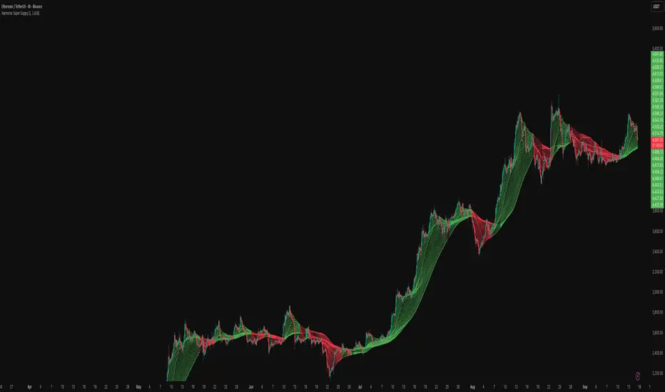
Harmonic Super GuppyHarmonic Super Guppy – Harmonic & Golden Ratio Trend Analysis Framework
Overview
Harmonic Super Guppy is a comprehensive trend analysis and visualization tool that evolves the classic Guppy Multiple Moving Average (GMMA) methodology, pioneered by Daryl Guppy to visualize the interaction between short-term trader behavior and long-term investor trends. into a harmonic and phase-based market framework. By combining harmonic weighting, golden ratio phasing, and multiple moving averages, it provides traders with a deep understanding of market structure, momentum, and trend alignment. Fast and slow line groups visually differentiate short-term trader activity from longer-term investor positioning, while adaptive fills and dynamic coloring clearly illustrate trend coherence, expansion, and contraction in real time.
Traditional GMMA focuses primarily on moving average convergence and divergence. Harmonic Super Guppy extends this concept, integrating frequency-aware harmonic analysis and golden ratio modulation, allowing traders to detect subtle cyclical forces and early trend shifts before conventional moving averages would react. This is particularly valuable for traders seeking to identify early trend continuation setups, preemptive breakout entries, and potential trend exhaustion zones. The indicator provides a multi-dimensional view, making it suitable for scalping, intraday trading, swing setups, and even longer-term position strategies.
The visual structure of Harmonic Super Guppy is intentionally designed to convey trend clarity without oversimplification. Fast lines reflect short-term trader sentiment, slow lines capture longer-term investor alignment, and fills highlight compression or expansion. The adaptive color coding emphasizes trend alignment: strong green for bullish alignment, strong red for bearish, and subtle gray tones for indecision. This allows traders to quickly gauge market conditions while preserving the granularity necessary for sophisticated analysis.
How It Works
Harmonic Super Guppy uses a combination of harmonic averaging, golden ratio phasing, and adaptive weighting to generate its signals.
Harmonic Weighting : Each moving average integrates three layers of harmonics:
Primary harmonic captures the dominant cyclical structure of the market.
Secondary harmonic introduces a complementary frequency for oscillatory nuance.
Tertiary harmonic smooths higher-frequency noise while retaining meaningful trend signals.
Golden Ratio Phase : Phases of each harmonic contribution are adjusted using the golden ratio (default φ = 1.618), ensuring alignment with natural market rhythms. This reduces lag and allows traders to detect trend shifts earlier than conventional moving averages.
Adaptive Trend Detection : Fast SMAs are compared against slow SMAs to identify structural trends:
UpTrend : Fast SMA exceeds slow SMA.
DownTrend : Fast SMA falls below slow SMA.
Frequency Scaling : The wave frequency setting allows traders to modulate responsiveness versus smoothing. Higher frequency emphasizes short-term moves, while lower frequency highlights structural trends. This enables adaptation across asset classes with different volatility characteristics.
Through this combination, Harmonic Super Guppy captures micro and macro market cycles, helping traders distinguish between transient noise and genuine trend development. The multi-harmonic approach amplifies meaningful price action while reducing false signals inherent in standard moving averages.
Interpretation
Harmonic Super Guppy provides a multi-dimensional perspective on market dynamics:
Trend Analysis : Alignment of fast and slow lines reveals trend direction and strength. Expanding harmonics indicate momentum building, while contraction signals weakening conditions or potential reversals.
Momentum & Volatility : Rapid expansion of fast lines versus slow lines reflects short-term bullish or bearish pressure. Compression often precedes breakout scenarios or volatility expansion. Traders can quickly gauge trend vigor and potential turning points.
Market Context : The indicator overlays harmonic and structural insights without dictating entry or exit points. It complements order blocks, liquidity zones, oscillators, and other technical frameworks, providing context for informed decision-making.
Phase Divergence Detection : Subtle divergence between harmonic layers (primary, secondary, tertiary) often signals early exhaustion in trends or hidden strength, offering preemptive insight into potential reversals or sustained continuation.
By observing both structural alignment and harmonic expansion/contraction, traders gain a clear sense of when markets are trending with conviction versus when conditions are consolidating or becoming unpredictable. This allows for proactive trade management, rather than reactive responses to lagging indicators.
Strategy Integration
Harmonic Super Guppy adapts to various trading methodologies with clear, actionable guidance.
Trend Following : Enter positions when fast and slow lines are aligned and harmonics are expanding. The broader the alignment, the stronger the confirmation of trend persistence. For example:
A fast line crossover above slow lines with expanding fills confirms momentum-driven continuation.
Traders can use harmonic amplitude as a filter to reduce entries against prevailing trends.
Breakout Trading : Periods of line compression indicate potential volatility expansion. When fast lines diverge from slow lines after compression, this often precedes breakouts. Traders can combine this visual cue with structural supports/resistances or order flow analysis to improve timing and precision.
Exhaustion and Reversals : Divergences between harmonic components, or contraction of fast lines relative to slow lines, highlight weakening trends. This can indicate liquidity exhaustion, trend fatigue, or corrective phases. For example:
A flattening fast line group above a rising slow line can hint at short-term overextension.
Traders may use these signals to tighten stops, take partial profits, or prepare for contrarian setups.
Multi-Timeframe Analysis : Overlay slow lines from higher timeframes on lower timeframe charts to filter noise and trade in alignment with larger market structures. For example:
A daily bullish alignment combined with a 15-minute breakout pattern increases probability of a successful intraday trade.
Conversely, a higher timeframe divergence can warn against taking counter-trend trades in lower timeframes.
Adaptive Trade Management : Harmonic expansion/contraction can guide dynamic risk management:
Stops may be adjusted according to slow line support/resistance or harmonic contraction zones.
Position sizing can be modulated based on harmonic amplitude and compression levels, optimizing risk-reward without rigid rules.
Technical Implementation Details
Harmonic Super Guppy is powered by a multi-layered harmonic and phase calculation engine:
Harmonic Processing : Primary, secondary, and tertiary harmonics are calculated per period to capture multiple market cycles simultaneously. This reduces noise and amplifies meaningful signals.
Golden Ratio Modulation : Phase adjustments based on φ = 1.618 align harmonic contributions with natural market rhythms, smoothing lag and improving predictive value.
Adaptive Trend Scaling : Fast line expansion reflects short-term momentum; slow lines provide structural trend context. Fills adapt dynamically based on alignment intensity and harmonic amplitude.
Multi-Factor Trend Analysis : Trend strength is determined by alignment of fast and slow lines over multiple bars, expansion/contraction of harmonic amplitudes, divergences between primary, secondary, and tertiary harmonics and phase synchronization with golden ratio cycles.
These computations allow the indicator to be highly responsive yet smooth, providing traders with actionable insights in real time without overloading visual complexity.
Optimal Application Parameters
Asset-Specific Guidance:
Forex Majors : Wave frequency 1.0–2.0, φ = 1.618–1.8
Large-Cap Equities : Wave frequency 0.8–1.5, φ = 1.5–1.618
Cryptocurrency : Wave frequency 1.2–3.0, φ = 1.618–2.0
Index Futures : Wave frequency 0.5–1.5, φ = 1.618
Timeframe Optimization:
Scalping (1–5min) : Emphasize fast lines, higher frequency for micro-move capture.
Day Trading (15min–1hr) : Balance fast/slow interactions for trend confirmation.
Swing Trading (4hr–Daily) : Focus on slow lines for structural guidance, fast lines for entry timing.
Position Trading (Daily–Weekly) : Slow lines dominate; harmonics highlight long-term cycles.
Performance Characteristics
High Effectiveness Conditions:
Clear separation between short-term and long-term trends.
Moderate-to-high volatility environments.
Assets with consistent volume and price rhythm.
Reduced Effectiveness:
Flat or extremely low volatility markets.
Erratic assets with frequent gaps or algorithmic dominance.
Ultra-short timeframes (<1min), where noise dominates.
Integration Guidelines
Signal Confirmation : Confirm alignment of fast and slow lines over multiple bars. Expansion of harmonic amplitude signals trend persistence.
Risk Management : Place stops beyond slow line support/resistance. Adjust sizing based on compression/expansion zones.
Advanced Feature Settings :
Frequency tuning for different volatility environments.
Phase analysis to track divergences across harmonics.
Use fills and amplitude patterns as a guide for dynamic trade management.
Multi-timeframe confirmation to filter noise and align with structural trends.
Disclaimer
Harmonic Super Guppy is a trend analysis and visualization tool, not a guaranteed profit system. Optimal performance requires proper wave frequency, golden ratio phase, and line visibility settings per asset and timeframe. Traders should combine the indicator with other technical frameworks and maintain disciplined risk management practices.
在腳本中搜尋"technical"
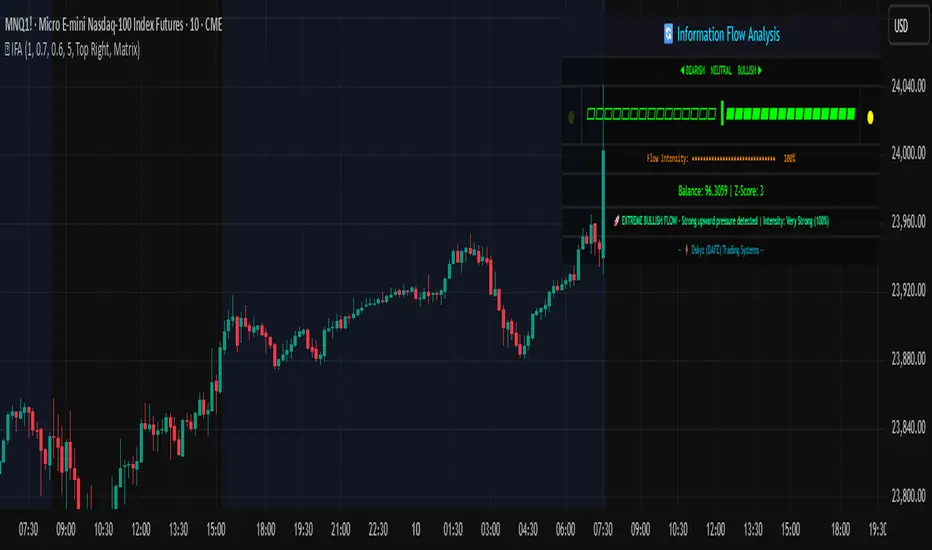
Information Flow Analysis[b🔄 Information Flow Analysis: Systematic Multi-Component Market Analysis Framework
SYSTEM OVERVIEW AND ANALYTICAL FOUNDATION
The Information Flow Kernel - Hybrid combines established technical analysis methods into a unified analytical framework. This indicator systematically processes three distinct data streams - directional price momentum, volume-weighted pressure dynamics, and intrabar development patterns - integrating them through weighted mathematical fusion to produce statistically normalized market flow measurements.
COMPREHENSIVE MATHEMATICAL FRAMEWORK
Component 1: Directional Flow Analysis
The directional component analyzes price momentum through three mathematical vectors:
Price Vector: p = C - O (intrabar directional bias)
Momentum Vector: m = C_t - C_{t-1} (bar-to-bar velocity)
Acceleration Vector: a = m_t - m_{t-1} (momentum rate of change)
Directional Signal Integration:
S_d = \text{sgn}(p) \cdot |p| + \text{sgn}(m) \cdot |m| \cdot 0.6 + \text{sgn}(a) \cdot |a| \cdot 0.3
The signum function preserves directional information while absolute values provide magnitude weighting. Coefficients create a hierarchy emphasizing intrabar movement (100%), momentum (60%), and acceleration (30%).
Final Directional Output: K_1 = S_d \cdot w_d where w_d is the directional weight parameter.
Component 2: Volume-Weighted Pressure Analysis
Volume Normalization: r_v = \frac{V_t}{\overline{V_n}} where \overline{V_n} represents the n-period simple moving average of volume.
Base Pressure Calculation: P_{base} = \Delta C \cdot r_v \cdot w_v where \Delta C = C_t - C_{t-1} and w_v is the velocity weighting factor.
Volume Confirmation Function:
f(r_v) = \begin{cases}
1.4 & \text{if } r_v > 1.2 \
0.7 & \text{if } r_v < 0.8 \
1.0 & \text{otherwise}
\end{cases}
Final Pressure Output: K_2 = P_{base} \cdot f(r_v)
Component 3: Intrabar Development Analysis
Bar Position Calculation: B = \frac{C - L}{H - L} when H - L > 0 , else B = 0.5
Development Signal Function:
S_{dev} = \begin{cases}
2(B - 0.5) & \text{if } B > 0.6 \text{ or } B < 0.4 \
0 & \text{if } 0.4 \leq B \leq 0.6
\end{cases}
Final Development Output: K_3 = S_{dev} \cdot 0.4
Master Integration and Statistical Normalization
Weighted Component Fusion: F_{raw} = 0.5K_1 + 0.35K_2 + 0.15K_3
Sensitivity Scaling: F_{master} = F_{raw} \cdot s where s is the sensitivity parameter.
Statistical Normalization Process:
Rolling Mean: \mu_F = \frac{1}{n}\sum_{i=0}^{n-1} F_{master,t-i}
Rolling Standard Deviation: \sigma_F = \sqrt{\frac{1}{n}\sum_{i=0}^{n-1} (F_{master,t-i} - \mu_F)^2}
Z-Score Computation: z = \frac{F_{master} - \mu_F}{\sigma_F}
Boundary Enforcement: z_{bounded} = \max(-3, \min(3, z))
Final Normalization: N = \frac{z_{bounded}}{3}
Flow Metrics Calculation:
Intensity: I = |z|
Strength Percentage: S = \min(100, I \times 33.33)
Extreme Detection: \text{Extreme} = I > 2.0
DETAILED INPUT PARAMETER SPECIFICATIONS
Sensitivity (0.1 - 3.0, Default: 1.0)
Global amplification multiplier applied to the master flow calculation. Functions as: F_{master} = F_{raw} \cdot s
Low Settings (0.1 - 0.5): Enhanced precision for subtle market movements. Optimal for low-volatility environments, scalping strategies, and early detection of minor directional shifts. Increases responsiveness but may amplify noise.
Moderate Settings (0.6 - 1.2): Balanced sensitivity for standard market conditions across multiple timeframes.
High Settings (1.3 - 3.0): Reduced sensitivity to minor fluctuations while emphasizing significant flow changes. Ideal for high-volatility assets, trending markets, and longer timeframes.
Directional Weighting (0.1 - 1.0, Default: 0.7)
Controls emphasis on price direction versus volume and positioning factors. Applied as: K_{1,weighted} = K_1 \times w_d
Lower Values (0.1 - 0.4): Reduces directional bias, favoring volume-confirmed moves. Optimal for ranging markets where momentum may generate false signals.
Higher Values (0.7 - 1.0): Amplifies directional signals from price vectors and acceleration. Ideal for trending conditions where directional momentum drives price action.
Velocity Weighting (0.1 - 1.0, Default: 0.6)
Scales volume-confirmed price change impact. Applied in: P_{base} = \Delta C \times r_v \times w_v
Lower Values (0.1 - 0.4): Dampens volume spike influence, focusing on sustained pressure patterns. Suitable for illiquid assets or news-sensitive markets.
Higher Values (0.8 - 1.0): Amplifies high-volume directional moves. Optimal for liquid markets where volume provides reliable confirmation.
Volume Length (3 - 20, Default: 5)
Defines lookback period for volume averaging: \overline{V_n} = \frac{1}{n}\sum_{i=0}^{n-1} V_{t-i}
Short Periods (3 - 7): Responsive to recent volume shifts, excellent for intraday analysis.
Long Periods (13 - 20): Smoother averaging, better for swing trading and higher timeframes.
DASHBOARD SYSTEM
Primary Flow Gauge
Bilaterally symmetric visualization displaying normalized flow direction and intensity:
Segment Calculation: n_{active} = \lfloor |N| \times 15 \rfloor
Left Fill: Bearish flow when N < -0.01
Right Fill: Bullish flow when N > 0.01
Neutral Display: Empty segments when |N| \leq 0.01
Visual Style Options:
Matrix: Digital blocks (▰/▱) for quantitative precision
Wave: Progressive patterns (▁▂▃▄▅▆▇█) showing flow buildup
Dots: LED-style indicators (●/○) with intensity scaling
Blocks: Modern squares (■/□) for professional appearance
Pulse: Progressive markers (⎯ to █) emphasizing intensity buildup
Flow Intensity Visualization
30-segment horizontal bar graph with mathematical fill logic:
Segment Fill: For i \in : filled if \frac{i}{29} \leq \frac{S}{100}
Color Coding System:
Orange (S > 66%): High intensity, strong directional conviction
Cyan (33% ≤ S ≤ 66%): Moderate intensity, developing bias
White (S < 33%): Low intensity, neutral conditions
Extreme Detection Indicators
Circular markers flanking the gauge with state-dependent illumination:
Activation: I > 2.0 \land |N| > 0.3
Bright Yellow: Active extreme conditions
Dim Yellow: Normal conditions
Metrics Display
Balance Value: Raw master flow output ( F_{master} ) showing absolute directional pressure
Z-Score Value: Statistical deviation ( z_{bounded} ) indicating historical context
Dynamic Narrative System
Context-sensitive interpretation based on mathematical thresholds:
Extreme Flow: I > 2.0 \land |N| > 0.6
Moderate Flow: 0.3 < |N| \leq 0.6
High Volatility: S > 50 \land |N| \leq 0.3
Neutral State: S \leq 50 \land |N| \leq 0.3
ALERT SYSTEM SPECIFICATIONS
Mathematical Trigger Conditions:
Extreme Bullish: I > 2.0 \land N > 0.6
Extreme Bearish: I > 2.0 \land N < -0.6
High Intensity: S > 80
Bullish Shift: N_t > 0.3 \land N_{t-1} \leq 0.3
Bearish Shift: N_t < -0.3 \land N_{t-1} \geq -0.3
TECHNICAL IMPLEMENTATION AND PERFORMANCE
Computational Architecture
The system employs efficient calculation methods minimizing processing overhead:
Single-pass mathematical operations for all components
Conditional visual rendering (executed only on final bar)
Optimized array operations using direct calculations
Real-Time Processing
The indicator updates continuously during bar formation, providing immediate feedback on changing market conditions. Statistical normalization ensures consistent interpretation across varying market regimes.
Market Applicability
Optimal performance in liquid markets with consistent volume patterns. May require parameter adjustment for:
Low-volume or after-hours sessions
News-driven market conditions
Highly volatile cryptocurrency markets
Ranging versus trending market environments
PRACTICAL APPLICATION FRAMEWORK
Market State Classification
This indicator functions as a comprehensive market condition assessment tool providing:
Trend Analysis: High intensity readings ( S > 66% ) with sustained directional bias indicate strong trending conditions suitable for momentum strategies.
Reversal Detection: Extreme readings ( I > 2.0 ) at key technical levels may signal potential trend exhaustion or reversal points.
Range Identification: Low intensity with neutral flow ( S < 33%, |N| < 0.3 ) suggests ranging market conditions suitable for mean reversion strategies.
Volatility Assessment: High intensity without clear directional bias indicates elevated volatility with conflicting pressures.
Integration with Trading Systems
The normalized output range facilitates integration with automated trading systems and position sizing algorithms. The statistical basis provides consistent interpretation across different market conditions and asset classes.
LIMITATIONS AND CONSIDERATIONS
This indicator combines established technical analysis methods and processes historical data without predicting future price movements. The system performs optimally in liquid markets with consistent volume patterns and may produce false signals in thin trading conditions or during news-driven market events. This indicator is provided for educational and analytical purposes only and does not constitute financial advice. Users should combine this analysis with proper risk management, position sizing, and additional confirmation methods before making any trading decisions. Past performance does not guarantee future results.
Note: The term "kernel" in this context refers to modular calculation components rather than mathematical kernel functions in the formal computational sense.
As quantitative analyst Ralph Vince noted: "The essence of successful trading lies not in predicting market direction, but in the systematic processing of market information and the disciplined management of probability distributions."
— Dskyz, Trade with insight. Trade with anticipation.
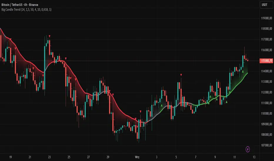
Big Candle Trend█ OVERVIEW
The "Big Candle Trend" indicator is a technical analysis tool written in Pine Script® v6 that identifies large signal candles on the chart and determines the trend direction based on the analysis of all candles within a specified period. Designed for traders seeking a simple yet effective tool to identify key market movements and trends, the indicator provides clarity and precision through flexible settings, trend line visualization, and retracement lines on signal candles.
█ CONCEPTS
The goal of the "Big Candle Trend" indicator was to create a tool based solely on the size of candle bodies and their relative positions, making it universal and effective across all markets (stocks, forex, cryptocurrencies) and timeframes. Unlike traditional indicators that often rely on complex formulas or external data (e.g., volume), this indicator uses simple yet powerful price action logic. Large signal candles are identified by comparing their body size to the average body size over a selected period, and the trend is determined by analyzing price changes over a longer period relative to the average candle body size. Additionally, the indicator draws horizontal lines on signal candles, aiding in setting Stop Loss levels or delayed entries.
█ FEATURES
Large Signal Candle Detection: Identifies candles with a body larger than the average body multiplied by a user-defined multiplier, aligned with the trend (if the trend filter is enabled). Signals are displayed as triangles (green for bullish, red for bearish).
Trend Analysis: Determines the trend (uptrend, downtrend, or neutral) by comparing the price change over a selected period (trend_length) to the average candle body size multiplied by a trend strength multiplier. The trend starts when:
Uptrend: The price change (difference between the current close and the close from an earlier period) is positive and exceeds the average candle body size multiplied by the trend strength multiplier (avg_body_trend * trend_mult).
Downtrend: The price change is negative and exceeds, in absolute value, the average candle body size multiplied by the trend strength multiplier.
Neutral Trend: The price change is below the required threshold, indicating no clear market direction.The trend ends when the price change no longer meets the conditions for an uptrend or downtrend, transitioning to a neutral state or switching to the opposite trend when the price change reverses and meets the conditions for the new trend. This approach differs from standard methods as it focuses on price dynamics in the context of candle body size, offering a more intuitive and direct way to gauge trend strength.
Smoothed Trend Line: Displays a trend line based on the average price (HL2, i.e., the average of the high and low of a candle), smoothed using a user-defined smoothing parameter. The trend line reflects the market direction but is not tied to breakouts, unlike many other trend indicators, allowing for more flexible interpretation.
Retracement Lines: Draws horizontal lines on signal candles at a user-defined level (e.g., 0.618). The lines are displayed to the right of the candle, with a width of one candle. For bullish candles, the line is measured from the top of the body (close) downward, and for bearish candles, from the bottom of the body (close) upward, aiding in setting Stop Loss or delayed entries.
Trend Option: Option to enable a trend filter that limits large candle signals to those aligned with the current trend, enhancing signal precision.
Customizable Visualization: Allows customization of colors for uptrend, downtrend, and neutral states, trend line style, and shadow fill between the trend line and price.
Alerts: Built-in alerts for large signal candles (bullish and bearish) and trend changes (start of uptrend, downtrend, or neutral trend).
█ HOW TO USE
Add to Chart: Apply the indicator to your TradingView chart via the Pine Editor or Indicators menu.
Configure Settings:
Candle Settings:
Average Period (Candles): Sets the period for calculating the average candle body size.
Large Candle Multiplier: Multiplier determining how large a candle’s body must be to be considered "large".
Trend Settings:
Trend Period: Period for analyzing price changes to determine the trend.
Trend Strength Multiplier: Multiplier setting the minimum price change required to identify a significant trend.
Trend Line Smoothing: Degree of smoothing for the trend line.
Show Trend Line: Enables/disables the display of the trend line.
Apply Trend Filter: Limits large candle signals to those aligned with the current trend.
Trend Colors:
Customize colors for uptrend (green), downtrend (red), and neutral (gray) states, and enable/disable shadow fill.
Retracement Settings:
Retracement Level (0.0-1.0): Sets the level for lines on signal candles (e.g., 0.618).
Line Width: Sets the thickness of retracement lines.
Interpreting Signals:
Bullish Signal: A green triangle below the candle indicates a large bullish candle aligned with an uptrend (if the trend filter is enabled). A horizontal line is drawn to the right of the candle at the retracement level, measured from the top of the body downward.
Bearish Signal: A red triangle above the candle indicates a large bearish candle aligned with a downtrend (if the trend filter is enabled). A horizontal line is drawn to the right of the candle at the retracement level, measured from the bottom of the body upward.
rend Line: Shows the market direction (green for uptrend, red for downtrend, gray for neutral). Unlike many indicators, the trend line’s color is not tied to its breakout, allowing for more flexible interpretation of market dynamics.
Alerts: Set up alerts in TradingView for large signal candles or trend changes to receive real-time notifications.
Combining with Other Tools: Use the indicator alongside other technical analysis tools, such as support/resistance levels, RSI, moving averages, or Fair Value Gaps (FVG), to confirm signals.
█ APPLICATIONS
Price Action Trading: Large signal candles can indicate key market moments, such as breakouts of support/resistance levels or strong price rejections. Use signal candles in conjunction with support/resistance levels or FVG to identify entry opportunities. Retracement lines help set Stop Loss levels (e.g., below the line for bullish candles, above for bearish) or delayed entries after price returns to the retracement level and confirms trend continuation. Note that large candles often generate Fair Value Gaps (FVG), which should be considered when setting Stop Loss levels.
Trend Strategies: Enable the trend filter to limit signals to those aligned with the dominant market direction. For example, in an uptrend, look for large bullish candles as continuation signals. The indicator can also be used for position pyramiding, adding positions as subsequent large candles confirm trend continuation.
Practical Approach:
Large candles with high volume may indicate strong market participation, increasing signal reliability.
The trend line helps visually assess market direction and confirm large candle signals.
Retracement lines on signal candles aid in identifying key levels for Stop Loss or delayed entries.
█ NOTES
The indicator works across all markets and timeframes due to its universal logic based on candle body size and relative positioning.
Adjust settings (e.g., trend period, large candle multiplier, retracement level) to suit your trading style and timeframe.
Test the indicator on various markets (stocks, forex, cryptocurrencies) and timeframes to optimize its performance.
Use in conjunction with other technical analysis tools to enhance signal accuracy.
PE Rating by The Noiseless TraderPE Rating by The Noiseless Trader
This script analyzes a symbol’s Price-to-Earnings (P/E) ratio, using Diluted EPS (TTM) fundamentals directly from TradingView.
The script calculates the Price-to-Earnings ratio (P/E) using Diluted EPS (TTM) fundamentals. It then identifies:
PE High → the highest valuation point over a 3-year historical range.
PE Low → the lowest valuation point over a 3-year historical range.
PE Median → the midpoint between the two extremes, offering a fair-value benchmark.
PE (Int) → an additional intermediate low to track more recent undervaluation points. This is calculated based on lowest valuation point over a 1-year historical range
These levels are plotted directly on the chart as horizontal references, with markers showing the exact bars/dates when the extremes occurred. Candles corresponding to those days are also highlighted for context.
Bars corresponding to these extremes are highlighted (red = PE High, green = PE Low).
How it helps
Provides a historical valuation framework that complements technical analysis. We look for long opportunity or base formation near the PE Low and be cautious when stocks tends to trade near High PE.
We do not short the stock at High PE infact be cautious with long trades.
Helps identify whether current price action is happening near overvalued or undervalued zones.
Adds a long-term perspective to support swing trading and investing decisions. If a stock is coming from Low PE to Median PE and along with that if we get entry based on Classical strategies like Darvas Box, or HH-HL based on Dow Theory.
Offers a simple visual map of how far the market has moved from “cheap” to “expensive.”
This tool is best suited for long-term investors and swing traders who want to merge fundamentals with technical setups.
This indicator is designed as an educational tool to illustrate how valuation metrics (like earnings multiples) can be viewed alongside price action, helping traders connect fundamental context with technical execution in real market conditions.

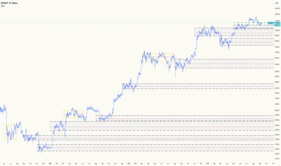
Composite Time ProfileComposite Time Profile Overlay (CTPO) - Market Profile Compositing Tool
Automatically composite multiple time periods to identify key areas of balance and market structure
What is the Composite Time Profile Overlay?
The Composite Time Profile Overlay (CTPO) is a Pine Script indicator that automatically composites multiple time periods to identify key areas of balance and market structure. It's designed for traders who use market profile concepts and need to quickly identify where price is likely to find support or resistance.
The indicator analyzes TPO (Time Price Opportunity) data across different timeframes and merges overlapping profiles to create composite levels that represent the most significant areas of balance. This helps you spot where institutional traders are likely to make decisions based on accumulated price action.
Why Use CTPO for Market Profile Trading?
Eliminate Manual Compositing Work
Instead of manually drawing and compositing profiles across different timeframes, CTPO does this automatically. You get instant access to composite levels without spending time analyzing each individual period.
Spot Areas of Balance Quickly
The indicator highlights the most significant areas of balance by compositing overlapping profiles. These areas often act as support and resistance levels because they represent where the most trading activity occurred across multiple time periods.
Focus on What Matters
Rather than getting lost in individual session profiles, CTPO shows you the composite levels that have been validated across multiple timeframes. This helps you focus on the levels that are most likely to hold.
How CTPO Works for Market Profile Traders
Automatic Profile Compositing
CTPO uses a proprietary algorithm that:
- Identifies period boundaries based on your selected timeframe (sessions, daily, weekly, monthly, or auto-detection)
- Calculates TPO profiles for each period using the C2M (Composite 2 Method) row sizing calculation
- Merges overlapping profiles using configurable overlap thresholds (default 50% overlap required)
- Updates composite levels as new price action develops in real-time
Key Levels for Market Profile Analysis
The indicator displays:
- Value Area High (VAH) and Value Area Low (VAL) levels calculated from composite TPO data
- Point of Control (POC) levels where most trading occurred across all composited periods
- Composite zones representing areas of balance with configurable transparency
- 1.618 Fibonacci extensions for breakout targets based on composite range
Multiple Timeframe Support
- Sessions: For intraday market profile analysis
- Daily: For swing trading with daily profiles
- Weekly: For position trading with weekly structure
- Monthly: For long-term market profile analysis
- Auto: Automatically selects timeframe based on your chart
Trading Applications for Market Profile Users
Support and Resistance Trading
Use composite levels as dynamic support and resistance zones. These levels often hold because they represent areas where significant trading decisions were made across multiple timeframes.
Breakout Trading
When composite levels break, they often lead to significant moves. The indicator calculates 1.618 Fibonacci extensions to give you clear targets for breakout trades.
Mean Reversion Strategies
Value Area levels represent the price range where most trading activity occurred. These levels often act as magnets, drawing price back when it moves too far from the mean.
Institutional Level Analysis
Composite levels represent areas where institutional traders have made significant decisions. These levels often hold more weight than traditional technical analysis levels because they're based on actual trading activity.
Key Features for Market Profile Traders
Smart Compositing Logic
- Automatic overlap detection using price range intersection algorithms
- Configurable overlap thresholds (minimum 50% overlap required for merging)
- Dead composite identification (profiles that become engulfed by newer composites)
- Real-time updates as new price action develops using barstate.islast optimization
Visual Customization
- Customizable colors for active, broken, and dead composites
- Adjustable transparency levels for each composite state
- Premium/Discount zone highlighting based on current price vs composite range
- TPO aggression coloring using TPO distribution analysis to identify buying/selling pressure
- Fibonacci level extensions with 1.618 target calculations based on composite range
Clean Chart Presentation
- Only shows the most relevant composite levels (maximum 10 active composites)
- Eliminates clutter from individual session profiles
- Focuses on areas of balance that matter most to current price action
Real-World Trading Examples
Day Trading with Session Composites
Use session-based composites to identify intraday areas of balance. The VAH and VAL levels often act as natural profit targets and stop-loss levels for scalping strategies.
Swing Trading with Daily Composites
Daily composites provide excellent swing trading levels. Look for price reactions at composite zones and use the 1.618 extensions for profit targets.
Position Trading with Weekly Composites
Weekly composites help identify major trend changes and long-term areas of balance. These levels often hold for months or even years.
Risk Management
Composite levels provide natural stop-loss levels. If a composite level breaks, it often signals a significant shift in market sentiment, making it an ideal place to exit losing positions.
Why Composite Levels Work
Composite levels work because they represent areas where significant trading decisions were made across multiple timeframes. When price returns to these levels, traders often remember the previous price action and make similar decisions, creating self-fulfilling prophecies.
The compositing process uses a proprietary algorithm that ensures only levels validated across multiple time periods are displayed. This means you're looking at levels that have proven their significance through actual market behavior, not just random technical levels.
Technical Foundation
The indicator uses TPO (Time Price Opportunity) data combined with price action analysis to identify areas of balance. The C2M row sizing method ensures accurate profile calculations, while the overlap detection algorithm (minimum 50% price range intersection) ensures only truly significant composites are displayed. The algorithm calculates row size based on ATR (Average True Range) divided by 10, then converts to tick size for precise level calculations.
How the Code Actually Works
1. Period Detection and ATR Calculation
The code first determines the appropriate timeframe based on your chart:
- 1m-5m charts: Session-based profiles
- 15m-2h charts: Daily profiles
- 4h charts: Weekly profiles
- 1D charts: Monthly profiles
For each period type, it calculates the number of bars needed for ATR calculation:
- Sessions: 540 minutes divided by chart timeframe
- Daily: 1440 minutes divided by chart timeframe
- Weekly: 7 days worth of minutes divided by chart timeframe
- Monthly: 30 days worth of minutes divided by chart timeframe
2. C2M Row Size Calculation
The code calculates True Range for each bar in the determined period:
- True Range = max(high-low, |high-prevClose|, |low-prevClose|)
- Averages all True Range values to get ATR
- Row Size = (ATR / 10) converted to tick size
- This ensures each TPO row represents a meaningful price movement
3. TPO Profile Generation
For each period, the code:
- Creates price levels from lowest to highest price in the range
- Each level is separated by the calculated row size
- Counts how many bars touch each price level (TPO count)
- Finds the level with highest count = Point of Control (POC)
- Calculates Value Area by expanding from POC until 68.27% of total TPO blocks are included
4. Overlap Detection Algorithm
When a new profile is created, the code checks if it overlaps with existing composites:
- Calculates overlap range = min(currentVAH, prevVAH) - max(currentVAL, prevVAL)
- Calculates current profile range = currentVAH - currentVAL
- Overlap percentage = (overlap range / current profile range) * 100
- If overlap >= 50%, profiles are merged into a composite
5. Composite Merging Logic
When profiles overlap, the code creates a new composite by:
- Taking the earliest start bar and latest end bar
- Using the wider VAH/VAL range (max of both profiles)
- Keeping the POC from the profile with more TPO blocks
- Marking the composite as "active" until price breaks through
6. Real-Time Updates
The code uses barstate.islast to optimize performance:
- Only recalculates on the last bar of each period
- Updates active composite with live price action if enabled
- Cleans up old composites to prevent memory issues
- Redraws all visual elements from scratch each bar
7. Visual Rendering System
The code uses arrays to manage drawing objects:
- Clears all lines/boxes arrays on every bar
- Iterates through composites array to redraw everything
- Uses different colors for active, broken, and dead composites
- Calculates 1.618 Fibonacci extensions for broken composites
Getting Started with CTPO
Step 1: Choose Your Timeframe
Select the period type that matches your trading style:
- Use "Sessions" for day trading
- Use "Daily" for swing trading
- Use "Weekly" for position trading
- Use "Auto" to let the indicator choose based on your chart timeframe
Step 2: Customize the Display
Adjust colors, transparency, and display options to match your charting preferences. The indicator offers extensive customization options to ensure it fits seamlessly into your existing analysis.
Step 3: Identify Key Levels
Look for:
- Composite zones (blue boxes) - major areas of balance
- VAH/VAL lines - value area boundaries
- POC lines - areas of highest trading activity
- 1.618 extension lines - breakout targets
Step 4: Develop Your Strategy
Use these levels to:
- Set entry points near composite zones
- Place stop losses beyond composite levels
- Take profits at 1.618 extension levels
- Identify trend changes when major composites break
Perfect for Market Profile Traders
If you're already using market profile concepts in your trading, CTPO eliminates the manual work of compositing profiles across different timeframes. Instead of spending time analyzing each individual period, you get instant access to the composite levels that matter most.
The indicator's automated compositing process ensures you're always looking at the most relevant areas of balance, while its real-time updates keep you informed of changes as they happen. Whether you're a day trader looking for intraday levels or a position trader analyzing long-term structure, CTPO provides the market profile intelligence you need to succeed.
Streamline Your Market Profile Analysis
Stop wasting time on manual compositing. Let CTPO do the heavy lifting while you focus on executing profitable trades based on areas of balance that actually matter.
Ready to Streamline Your Market Profile Trading?
Add the Composite Time Profile Overlay to your charts today and experience the difference that automated profile compositing can make in your trading performance.
High Probability Order Blocks [AlgoAlpha]🟠 OVERVIEW
This script detects and visualizes high-probability order blocks by combining a volatility-based z-score trigger with a statistical survival model inspired by Kaplan-Meier estimation. It builds and manages bullish and bearish order blocks dynamically on the chart, displays live survival probabilities per block, and plots optional rejection signals. What makes this tool unique is its use of historical mitigation behavior to estimate and plot how likely each zone is to persist, offering traders a probabilistic perspective on order block strength—something rarely seen in retail indicators.
🟠 CONCEPTS
Order blocks are regions of strong institutional interest, often marked by large imbalances between buying and selling. This script identifies those areas using z-score thresholds on directional distance (up or down candles), detecting statistically significant moves that signal potential smart money footprints. A bullish block is drawn when a strong up-move (zUp > 4) follows a down candle, and vice versa for bearish blocks. Over time, each block is evaluated: if price “mitigates” it (i.e., closes cleanly past the opposite side and confirmed with a 1 bar delay), it’s considered resolved and logged. These resolved blocks then inform a Kaplan-Meier-like survival curve, estimating the likelihood that future blocks of a given age will remain unbroken. The indicator then draws a probability curve for each side (bull/bear), updating it in real time.
🟠 FEATURES
Live label inside each block showing survival probability or “N.E.D.” if insufficient data.
Kaplan-Meier survival curves drawn directly on the chart to show estimated strength decay.
Rejection markers (▲ ▼) if price bounces cleanly off an active order block.
Alerts for zone creation and rejection signals, supporting rule-based trading workflows.
🟠 USAGE
Read the label inside each block for Age | Survival% (or N.E.D. if there aren’t enough samples yet); higher survival % suggests blocks of that age have historically lasted longer.
Use the right-side survival curves to gauge how probability decays with age for bull vs bear blocks, and align entries with the side showing stronger survival at current age.
Treat ▲ (bullish rejection) and ▼ (bearish rejection) as optional confluence when price tests a boundary and fails to break.
Turn on alerts for “Bullish Zone Created,” “Bearish Zone Created,” and rejection signals so you don’t need to watch constantly.
If your chart gets crowded, enable Prevent Overlap ; tune Max Box Age to your timeframe; and adjust KM Training Window / Minimum Samples to trade off responsiveness vs stability.

Tzotchev Trend Measure [EdgeTools]Are you still measuring trend strength with moving averages? Here is a better variant at scientific level:
Tzotchev Trend Measure: A Statistical Approach to Trend Following
The Tzotchev Trend Measure represents a sophisticated advancement in quantitative trend analysis, moving beyond traditional moving average-based indicators toward a statistically rigorous framework for measuring trend strength. This indicator implements the methodology developed by Tzotchev et al. (2015) in their seminal J.P. Morgan research paper "Designing robust trend-following system: Behind the scenes of trend-following," which introduced a probabilistic approach to trend measurement that has since become a cornerstone of institutional trading strategies.
Mathematical Foundation and Statistical Theory
The core innovation of the Tzotchev Trend Measure lies in its transformation of price momentum into a probability-based metric through the application of statistical hypothesis testing principles. The indicator employs the fundamental formula ST = 2 × Φ(√T × r̄T / σ̂T) - 1, where ST represents the trend strength score bounded between -1 and +1, Φ(x) denotes the normal cumulative distribution function, T represents the lookback period in trading days, r̄T is the average logarithmic return over the specified period, and σ̂T represents the estimated daily return volatility.
This formulation transforms what is essentially a t-statistic into a probabilistic trend measure, testing the null hypothesis that the mean return equals zero against the alternative hypothesis of non-zero mean return. The use of logarithmic returns rather than simple returns provides several statistical advantages, including symmetry properties where log(P₁/P₀) = -log(P₀/P₁), additivity characteristics that allow for proper compounding analysis, and improved validity of normal distribution assumptions that underpin the statistical framework.
The implementation utilizes the Abramowitz and Stegun (1964) approximation for the normal cumulative distribution function, achieving accuracy within ±1.5 × 10⁻⁷ for all input values. This approximation employs Horner's method for polynomial evaluation to ensure numerical stability, particularly important when processing large datasets or extreme market conditions.
Comparative Analysis with Traditional Trend Measurement Methods
The Tzotchev Trend Measure demonstrates significant theoretical and empirical advantages over conventional trend analysis techniques. Traditional moving average-based systems, including simple moving averages (SMA), exponential moving averages (EMA), and their derivatives such as MACD, suffer from several fundamental limitations that the Tzotchev methodology addresses systematically.
Moving average systems exhibit inherent lag bias, as documented by Kaufman (2013) in "Trading Systems and Methods," where he demonstrates that moving averages inevitably lag price movements by approximately half their period length. This lag creates delayed signal generation that reduces profitability in trending markets and increases false signal frequency during consolidation periods. In contrast, the Tzotchev measure eliminates lag bias by directly analyzing the statistical properties of return distributions rather than smoothing price levels.
The volatility normalization inherent in the Tzotchev formula addresses a critical weakness in traditional momentum indicators. As shown by Bollinger (2001) in "Bollinger on Bollinger Bands," momentum oscillators like RSI and Stochastic fail to account for changing volatility regimes, leading to inconsistent signal interpretation across different market conditions. The Tzotchev measure's incorporation of return volatility in the denominator ensures that trend strength assessments remain consistent regardless of the underlying volatility environment.
Empirical studies by Hurst, Ooi, and Pedersen (2013) in "Demystifying Managed Futures" demonstrate that traditional trend-following indicators suffer from significant drawdowns during whipsaw markets, with Sharpe ratios frequently below 0.5 during challenging periods. The authors attribute these poor performance characteristics to the binary nature of most trend signals and their inability to quantify signal confidence. The Tzotchev measure addresses this limitation by providing continuous probability-based outputs that allow for more sophisticated risk management and position sizing strategies.
The statistical foundation of the Tzotchev approach provides superior robustness compared to technical indicators that lack theoretical grounding. Fama and French (1988) in "Permanent and Temporary Components of Stock Prices" established that price movements contain both permanent and temporary components, with traditional moving averages unable to distinguish between these elements effectively. The Tzotchev methodology's hypothesis testing framework specifically tests for the presence of permanent trend components while filtering out temporary noise, providing a more theoretically sound approach to trend identification.
Research by Moskowitz, Ooi, and Pedersen (2012) in "Time Series Momentum in the Cross Section of Asset Returns" found that traditional momentum indicators exhibit significant variation in effectiveness across asset classes and time periods. Their study of multiple asset classes over decades revealed that simple price-based momentum measures often fail to capture persistent trends in fixed income and commodity markets. The Tzotchev measure's normalization by volatility and its probabilistic interpretation provide consistent performance across diverse asset classes, as demonstrated in the original J.P. Morgan research.
Comparative performance studies conducted by AQR Capital Management (Asness, Moskowitz, and Pedersen, 2013) in "Value and Momentum Everywhere" show that volatility-adjusted momentum measures significantly outperform traditional price momentum across international equity, bond, commodity, and currency markets. The study documents Sharpe ratio improvements of 0.2 to 0.4 when incorporating volatility normalization, consistent with the theoretical advantages of the Tzotchev approach.
The regime detection capabilities of the Tzotchev measure provide additional advantages over binary trend classification systems. Research by Ang and Bekaert (2002) in "Regime Switches in Interest Rates" demonstrates that financial markets exhibit distinct regime characteristics that traditional indicators fail to capture adequately. The Tzotchev measure's five-tier classification system (Strong Bull, Weak Bull, Neutral, Weak Bear, Strong Bear) provides more nuanced market state identification than simple trend/no-trend binary systems.
Statistical testing by Jegadeesh and Titman (2001) in "Profitability of Momentum Strategies" revealed that traditional momentum indicators suffer from significant parameter instability, with optimal lookback periods varying substantially across market conditions and asset classes. The Tzotchev measure's statistical framework provides more stable parameter selection through its grounding in hypothesis testing theory, reducing the need for frequent parameter optimization that can lead to overfitting.
Advanced Noise Filtering and Market Regime Detection
A significant enhancement over the original Tzotchev methodology is the incorporation of a multi-factor noise filtering system designed to reduce false signals during sideways market conditions. The filtering mechanism employs four distinct approaches: adaptive thresholding based on current market regime strength, volatility-based filtering utilizing ATR percentile analysis, trend strength confirmation through momentum alignment, and a comprehensive multi-factor approach that combines all methodologies.
The adaptive filtering system analyzes market microstructure through price change relative to average true range, calculates volatility percentiles over rolling windows, and assesses trend alignment across multiple timeframes using exponential moving averages of varying periods. This approach addresses one of the primary limitations identified in traditional trend-following systems, namely their tendency to generate excessive false signals during periods of low volatility or sideways price action.
The regime detection component classifies market conditions into five distinct categories: Strong Bull (ST > 0.3), Weak Bull (0.1 < ST ≤ 0.3), Neutral (-0.1 ≤ ST ≤ 0.1), Weak Bear (-0.3 ≤ ST < -0.1), and Strong Bear (ST < -0.3). This classification system provides traders with clear, quantitative definitions of market regimes that can inform position sizing, risk management, and strategy selection decisions.
Professional Implementation and Trading Applications
The indicator incorporates three distinct trading profiles designed to accommodate different investment approaches and risk tolerances. The Conservative profile employs longer lookback periods (63 days), higher signal thresholds (0.2), and reduced filter sensitivity (0.5) to minimize false signals and focus on major trend changes. The Balanced profile utilizes standard academic parameters with moderate settings across all dimensions. The Aggressive profile implements shorter lookback periods (14 days), lower signal thresholds (-0.1), and increased filter sensitivity (1.5) to capture shorter-term trend movements.
Signal generation occurs through threshold crossover analysis, where long signals are generated when the trend measure crosses above the specified threshold and short signals when it crosses below. The implementation includes sophisticated signal confirmation mechanisms that consider trend alignment across multiple timeframes and momentum strength percentiles to reduce the likelihood of false breakouts.
The alert system provides real-time notifications for trend threshold crossovers, strong regime changes, and signal generation events, with configurable frequency controls to prevent notification spam. Alert messages are standardized to ensure consistency across different market conditions and timeframes.
Performance Optimization and Computational Efficiency
The implementation incorporates several performance optimization features designed to handle large datasets efficiently. The maximum bars back parameter allows users to control historical calculation depth, with default settings optimized for most trading applications while providing flexibility for extended historical analysis. The system includes automatic performance monitoring that generates warnings when computational limits are approached.
Error handling mechanisms protect against division by zero conditions, infinite values, and other numerical instabilities that can occur during extreme market conditions. The finite value checking system ensures data integrity throughout the calculation process, with fallback mechanisms that maintain indicator functionality even when encountering corrupted or missing price data.
Timeframe validation provides warnings when the indicator is applied to unsuitable timeframes, as the Tzotchev methodology was specifically designed for daily and higher timeframe analysis. This validation helps prevent misapplication of the indicator in contexts where its statistical assumptions may not hold.
Visual Design and User Interface
The indicator features eight professional color schemes designed for different trading environments and user preferences. The EdgeTools theme provides an institutional blue and steel color palette suitable for professional trading environments. The Gold theme offers warm colors optimized for commodities trading. The Behavioral theme incorporates psychology-based color contrasts that align with behavioral finance principles. The Quant theme provides neutral colors suitable for analytical applications.
Additional specialized themes include Ocean, Fire, Matrix, and Arctic variations, each optimized for specific visual preferences and trading contexts. All color schemes include automatic dark and light mode optimization to ensure optimal readability across different chart backgrounds and trading platforms.
The information table provides real-time display of key metrics including current trend measure value, market regime classification, signal strength, Z-score, average returns, volatility measures, filter threshold levels, and filter effectiveness percentages. This comprehensive dashboard allows traders to monitor all relevant indicator components simultaneously.
Theoretical Implications and Research Context
The Tzotchev Trend Measure addresses several theoretical limitations inherent in traditional technical analysis approaches. Unlike moving average-based systems that rely on price level comparisons, this methodology grounds trend analysis in statistical hypothesis testing, providing a more robust theoretical foundation for trading decisions.
The probabilistic interpretation of trend strength offers significant advantages over binary trend classification systems. Rather than simply indicating whether a trend exists, the measure quantifies the statistical confidence level associated with the trend assessment, allowing for more nuanced risk management and position sizing decisions.
The incorporation of volatility normalization addresses the well-documented problem of volatility clustering in financial time series, ensuring that trend strength assessments remain consistent across different market volatility regimes. This normalization is particularly important for portfolio management applications where consistent risk metrics across different assets and time periods are essential.
Practical Applications and Trading Strategy Integration
The Tzotchev Trend Measure can be effectively integrated into various trading strategies and portfolio management frameworks. For trend-following strategies, the indicator provides clear entry and exit signals with quantified confidence levels. For mean reversion strategies, extreme readings can signal potential turning points. For portfolio allocation, the regime classification system can inform dynamic asset allocation decisions.
The indicator's statistical foundation makes it particularly suitable for quantitative trading strategies where systematic, rules-based approaches are preferred over discretionary decision-making. The standardized output range facilitates easy integration with position sizing algorithms and risk management systems.
Risk management applications benefit from the indicator's ability to quantify trend strength and provide early warning signals of potential trend changes. The multi-timeframe analysis capability allows for the construction of robust risk management frameworks that consider both short-term tactical and long-term strategic market conditions.
Implementation Guide and Parameter Configuration
The practical application of the Tzotchev Trend Measure requires careful parameter configuration to optimize performance for specific trading objectives and market conditions. This section provides comprehensive guidance for parameter selection and indicator customization.
Core Calculation Parameters
The Lookback Period parameter controls the statistical window used for trend calculation and represents the most critical setting for the indicator. Default values range from 14 to 63 trading days, with shorter periods (14-21 days) providing more sensitive trend detection suitable for short-term trading strategies, while longer periods (42-63 days) offer more stable trend identification appropriate for position trading and long-term investment strategies. The parameter directly influences the statistical significance of trend measurements, with longer periods requiring stronger underlying trends to generate significant signals but providing greater reliability in trend identification.
The Price Source parameter determines which price series is used for return calculations. The default close price provides standard trend analysis, while alternative selections such as high-low midpoint ((high + low) / 2) can reduce noise in volatile markets, and volume-weighted average price (VWAP) offers superior trend identification in institutional trading environments where volume concentration matters significantly.
The Signal Threshold parameter establishes the minimum trend strength required for signal generation, with values ranging from -0.5 to 0.5. Conservative threshold settings (0.2 to 0.3) reduce false signals but may miss early trend opportunities, while aggressive settings (-0.1 to 0.1) provide earlier signal generation at the cost of increased false positive rates. The optimal threshold depends on the trader's risk tolerance and the volatility characteristics of the traded instrument.
Trading Profile Configuration
The Trading Profile system provides pre-configured parameter sets optimized for different trading approaches. The Conservative profile employs a 63-day lookback period with a 0.2 signal threshold and 0.5 noise sensitivity, designed for long-term position traders seeking high-probability trend signals with minimal false positives. The Balanced profile uses a 21-day lookback with 0.05 signal threshold and 1.0 noise sensitivity, suitable for swing traders requiring moderate signal frequency with acceptable noise levels. The Aggressive profile implements a 14-day lookback with -0.1 signal threshold and 1.5 noise sensitivity, optimized for day traders and scalpers requiring frequent signal generation despite higher noise levels.
Advanced Noise Filtering System
The noise filtering mechanism addresses the challenge of false signals during sideways market conditions through four distinct methodologies. The Adaptive filter adjusts thresholds based on current trend strength, increasing sensitivity during strong trending periods while raising thresholds during consolidation phases. The Volatility-based filter utilizes Average True Range (ATR) percentile analysis to suppress signals during abnormally volatile conditions that typically generate false trend indications.
The Trend Strength filter requires alignment between multiple momentum indicators before confirming signals, reducing the probability of false breakouts from consolidation patterns. The Multi-factor approach combines all filtering methodologies using weighted scoring to provide the most robust noise reduction while maintaining signal responsiveness during genuine trend initiations.
The Noise Sensitivity parameter controls the aggressiveness of the filtering system, with lower values (0.5-1.0) providing conservative filtering suitable for volatile instruments, while higher values (1.5-2.0) allow more signals through but may increase false positive rates during choppy market conditions.
Visual Customization and Display Options
The Color Scheme parameter offers eight professional visualization options designed for different analytical preferences and market conditions. The EdgeTools scheme provides high contrast visualization optimized for trend strength differentiation, while the Gold scheme offers warm tones suitable for commodity analysis. The Behavioral scheme uses psychological color associations to enhance decision-making speed, and the Quant scheme provides neutral colors appropriate for quantitative analysis environments.
The Ocean, Fire, Matrix, and Arctic schemes offer additional aesthetic options while maintaining analytical functionality. Each scheme includes optimized colors for both light and dark chart backgrounds, ensuring visibility across different trading platform configurations.
The Show Glow Effects parameter enhances plot visibility through multiple layered lines with progressive transparency, particularly useful when analyzing multiple timeframes simultaneously or when working with dense price data that might obscure trend signals.
Performance Optimization Settings
The Maximum Bars Back parameter controls the historical data depth available for calculations, with values ranging from 5,000 to 50,000 bars. Higher values enable analysis of longer-term trend patterns but may impact indicator loading speed on slower systems or when applied to multiple instruments simultaneously. The optimal setting depends on the intended analysis timeframe and available computational resources.
The Calculate on Every Tick parameter determines whether the indicator updates with every price change or only at bar close. Real-time calculation provides immediate signal updates suitable for scalping and day trading strategies, while bar-close calculation reduces computational overhead and eliminates signal flickering during bar formation, preferred for swing trading and position management applications.
Alert System Configuration
The Alert Frequency parameter controls notification generation, with options for all signals, bar close only, or once per bar. High-frequency trading strategies benefit from all signals mode, while position traders typically prefer bar close alerts to avoid premature position entries based on intrabar fluctuations.
The alert system generates four distinct notification types: Long Signal alerts when the trend measure crosses above the positive signal threshold, Short Signal alerts for negative threshold crossings, Bull Regime alerts when entering strong bullish conditions, and Bear Regime alerts for strong bearish regime identification.
Table Display and Information Management
The information table provides real-time statistical metrics including current trend value, regime classification, signal status, and filter effectiveness measurements. The table position can be customized for optimal screen real estate utilization, and individual metrics can be toggled based on analytical requirements.
The Language parameter supports both English and German display options for international users, while maintaining consistent calculation methodology regardless of display language selection.
Risk Management Integration
Effective risk management integration requires coordination between the trend measure signals and position sizing algorithms. Strong trend readings (above 0.5 or below -0.5) support larger position sizes due to higher probability of trend continuation, while neutral readings (between -0.2 and 0.2) suggest reduced position sizes or range-trading strategies.
The regime classification system provides additional risk management context, with Strong Bull and Strong Bear regimes supporting trend-following strategies, while Neutral regimes indicate potential for mean reversion approaches. The filter effectiveness metric helps traders assess current market conditions and adjust strategy parameters accordingly.
Timeframe Considerations and Multi-Timeframe Analysis
The indicator's effectiveness varies across different timeframes, with higher timeframes (daily, weekly) providing more reliable trend identification but slower signal generation, while lower timeframes (hourly, 15-minute) offer faster signals with increased noise levels. Multi-timeframe analysis combining trend alignment across multiple periods significantly improves signal quality and reduces false positive rates.
For optimal results, traders should consider trend alignment between the primary trading timeframe and at least one higher timeframe before entering positions. Divergences between timeframes often signal potential trend reversals or consolidation periods requiring strategy adjustment.
Conclusion
The Tzotchev Trend Measure represents a significant advancement in technical analysis methodology, combining rigorous statistical foundations with practical trading applications. Its implementation of the J.P. Morgan research methodology provides institutional-quality trend analysis capabilities previously available only to sophisticated quantitative trading firms.
The comprehensive parameter configuration options enable customization for diverse trading styles and market conditions, while the advanced noise filtering and regime detection capabilities provide superior signal quality compared to traditional trend-following indicators. Proper parameter selection and understanding of the indicator's statistical foundation are essential for achieving optimal trading results and effective risk management.
References
Abramowitz, M. and Stegun, I.A. (1964). Handbook of Mathematical Functions with Formulas, Graphs, and Mathematical Tables. Washington: National Bureau of Standards.
Ang, A. and Bekaert, G. (2002). Regime Switches in Interest Rates. Journal of Business and Economic Statistics, 20(2), 163-182.
Asness, C.S., Moskowitz, T.J., and Pedersen, L.H. (2013). Value and Momentum Everywhere. Journal of Finance, 68(3), 929-985.
Bollinger, J. (2001). Bollinger on Bollinger Bands. New York: McGraw-Hill.
Fama, E.F. and French, K.R. (1988). Permanent and Temporary Components of Stock Prices. Journal of Political Economy, 96(2), 246-273.
Hurst, B., Ooi, Y.H., and Pedersen, L.H. (2013). Demystifying Managed Futures. Journal of Investment Management, 11(3), 42-58.
Jegadeesh, N. and Titman, S. (2001). Profitability of Momentum Strategies: An Evaluation of Alternative Explanations. Journal of Finance, 56(2), 699-720.
Kaufman, P.J. (2013). Trading Systems and Methods. 5th Edition. Hoboken: John Wiley & Sons.
Moskowitz, T.J., Ooi, Y.H., and Pedersen, L.H. (2012). Time Series Momentum. Journal of Financial Economics, 104(2), 228-250.
Tzotchev, D., Lo, A.W., and Hasanhodzic, J. (2015). Designing robust trend-following system: Behind the scenes of trend-following. J.P. Morgan Quantitative Research, Asset Management Division.

Simplified Market ForecastSimplified Market Forecast Indicator
This indicator pairs nicely with the Contrarian 100 MA and can be located here:
Overview
The "Simplified Market Forecast" (SMF) indicator is a streamlined technical analysis tool designed for traders to identify potential buy and sell opportunities based on a momentum-based oscillator. By analyzing price movements relative to a defined lookback period, SMF generates clear buy and sell signals when the oscillator crosses customizable threshold levels. This indicator is versatile, suitable for various markets (e.g., forex, stocks, cryptocurrencies), and optimized for daily timeframes, though it can be adapted to other timeframes with proper testing. Its intuitive design and visual cues make it accessible for both novice and experienced traders.
How It Works
The SMF indicator calculates a momentum oscillator based on the price’s position within a specified range over a user-defined lookback period. It then smooths this value to reduce noise and plots the result as a line in a separate lower pane. Buy and sell signals are generated when the smoothed oscillator crosses above a user-defined buy level or below a user-defined sell level, respectively. These signals are visualized as triangles either on the main chart or in the lower pane, with a table displaying the current ticker and oscillator value for quick reference.
Key Components
Momentum Oscillator: The indicator measures the price’s position relative to the highest high and lowest low over a specified period, normalized to a 0–100 scale.
Signal Generation: Buy signals occur when the oscillator crosses above the buy level (default: 15), indicating potential oversold conditions. Sell signals occur when the oscillator crosses below the sell level (default: 85), suggesting potential overbought conditions.
Visual Aids: The indicator includes customizable horizontal lines for buy and sell levels, shaded zones for clarity, and a table showing the ticker and current oscillator value.
Mathematical Concepts
Oscillator Calculation: The indicator uses the following formula to compute the raw oscillator value:
c1I = close - lowest(low, medLen)
c2I = highest(high, medLen) - lowest(low, medLen)
fastK_I = (c1I / c2I) * 100
The result is smoothed using a 5-period Simple Moving Average (SMA) to produce the final oscillator value (inter).
Signal Logic:
A buy signal is triggered when the smoothed oscillator crosses above the buy level (ta.crossover(inter, buyLevel)).
A sell signal is triggered when the smoothed oscillator crosses below the sell level (ta.crossunder(inter, sellLevel)).
Entry and Exit Rules
Buy Signal (Blue Triangle): Triggered when the oscillator crosses above the buy level (default: 15), indicating a potential oversold condition and a buying opportunity. The signal appears as a blue triangle either below the price bar (if plotted on the main chart) or at the bottom of the lower pane.
Sell Signal (White Triangle): Triggered when the oscillator crosses below the sell level (default: 85), indicating a potential overbought condition and a selling opportunity. The signal appears as a white triangle either above the price bar (if plotted on the main chart) or at the top of the lower pane.
Exit Rules: Traders can exit positions when an opposite signal occurs (e.g., exit a buy on a sell signal) or based on additional technical analysis tools (e.g., support/resistance, trendlines). Always apply proper risk management.
Recommended Usage
The SMF indicator is optimized for the daily timeframe but can be adapted to other timeframes (e.g., 1H, 4H) with careful testing. It performs best in markets with clear momentum shifts, such as trending or range-bound conditions. Traders should:
Backtest the indicator on their chosen asset and timeframe to validate signal reliability.
Combine with other indicators (e.g., moving averages, support/resistance) or price action for confirmation.
Adjust the lookback period and buy/sell levels to suit market volatility and trading style.
Customization Options
Intermediate Length: Adjust the lookback period for the oscillator calculation (default: 31 bars).
Buy/Sell Levels: Customize the threshold levels for buy (default: 15) and sell (default: 85) signals.
Colors: Modify the colors of the oscillator line, buy/sell signals, and threshold lines.
Signal Display: Toggle whether signals appear on the main chart or in the lower pane.
Visual Aids: The indicator includes dotted horizontal lines at the buy (green) and sell (red) levels, with shaded zones between 0–buy level (green) and sell level–100 (red) for clarity.
Ticker Table: A table in the top-right corner displays the current ticker and oscillator value (in percentage), with customizable colors.
Why Use This Indicator?
The "Simplified Market Forecast" indicator provides a straightforward, momentum-based approach to identifying potential reversals in overbought or oversold markets. Its clear signals, customizable settings, and visual aids make it easy to integrate into various trading strategies. Whether you’re a swing trader or a day trader, SMF offers a reliable tool to enhance decision-making and improve market timing.
Tips for Users
Test the indicator thoroughly on your chosen asset and timeframe to optimize settings.
Use in conjunction with other technical tools for stronger trade confirmation.
Adjust the buy and sell levels based on market conditions (e.g., lower levels for less volatile markets).
Monitor the ticker table for real-time oscillator values to gauge market momentum.
Happy trading with the Simplified Market Forecast indicator!
[blackcat] L2 Trend LinearityOVERVIEW
The L2 Trend Linearity indicator is a sophisticated market analysis tool designed to help traders identify and visualize market trend linearity by analyzing price action relative to dynamic support and resistance zones. This powerful Pine Script indicator utilizes the Arnaud Legoux Moving Average (ALMA) algorithm to calculate weighted price calculations and generate dynamic support/resistance zones that adapt to changing market conditions. By visualizing market zones through colored candles and histograms, the indicator provides clear visual cues about market momentum and potential trading opportunities. The script generates buy/sell signals based on zone crossovers, making it an invaluable tool for both technical analysis and automated trading strategies. Whether you're a day trader, swing trader, or algorithmic trader, this indicator can help you identify market regimes, support/resistance levels, and potential entry/exit points with greater precision.
FEATURES
Dynamic Support/Resistance Zones: Calculates dynamic support (bear market zone) and resistance (bull market zone) using weighted price calculations and ALMA smoothing
Visual Market Representation: Color-coded candles and histograms provide immediate visual feedback about market conditions
Smart Signal Generation: Automatic buy/sell signals generated from zone crossovers with clear visual indicators
Customizable Parameters: Four different ALMA smoothing parameters for various timeframes and trading styles
Multi-Timeframe Compatibility: Works across different timeframes from 1-minute to weekly charts
Real-time Analysis: Provides instant feedback on market momentum and trend direction
Clear Visual Cues: Green candles indicate bullish momentum, red candles indicate bearish momentum, and white candles indicate neutral conditions
Histogram Visualization: Blue histogram shows bear market zone (below support), aqua histogram shows bull market zone (above resistance)
Signal Labels: "B" labels mark buy signals (price crosses above resistance), "S" labels mark sell signals (price crosses below support)
Overlay Functionality: Works as an overlay indicator without cluttering the chart with unnecessary elements
Highly Customizable: All parameters can be adjusted to suit different trading strategies and market conditions
HOW TO USE
Add the Indicator to Your Chart
Open TradingView and navigate to your desired trading instrument
Click on "Indicators" in the top menu and select "New"
Search for "L2 Trend Linearity" or paste the Pine Script code
Click "Add to Chart" to apply the indicator
Configure the Parameters
ALMA Length Short: Set the short-term smoothing parameter (default: 3). Lower values provide more responsive signals but may generate more false signals
ALMA Length Medium: Set the medium-term smoothing parameter (default: 5). This provides a balance between responsiveness and stability
ALMA Length Long: Set the long-term smoothing parameter (default: 13). Higher values provide more stable signals but with less responsiveness
ALMA Length Very Long: Set the very long-term smoothing parameter (default: 21). This provides the most stable support/resistance levels
Understand the Visual Elements
Green Candles: Indicate bullish momentum when price is above the bear market zone (support)
Red Candles: Indicate bearish momentum when price is below the bull market zone (resistance)
White Candles: Indicate neutral market conditions when price is between support and resistance zones
Blue Histogram: Shows bear market zone when price is below support level
Aqua Histogram: Shows bull market zone when price is above resistance level
"B" Labels: Mark buy signals when price crosses above resistance
"S" Labels: Mark sell signals when price crosses below support
Identify Market Regimes
Bullish Regime: Price consistently above resistance zone with green candles and aqua histogram
Bearish Regime: Price consistently below support zone with red candles and blue histogram
Neutral Regime: Price oscillating between support and resistance zones with white candles
Generate Trading Signals
Buy Signals: Look for price crossing above the bull market zone (resistance) with confirmation from green candles
Sell Signals: Look for price crossing below the bear market zone (support) with confirmation from red candles
Confirmation: Always wait for confirmation from candle color changes before entering trades
Optimize for Different Timeframes
Scalping: Use shorter ALMA lengths (3-5) for 1-5 minute charts
Day Trading: Use medium ALMA lengths (5-13) for 15-60 minute charts
Swing Trading: Use longer ALMA lengths (13-21) for 1-4 hour charts
Position Trading: Use very long ALMA lengths (21+) for daily and weekly charts
LIMITATIONS
Whipsaw Markets: The indicator may generate false signals in choppy, sideways markets where price oscillates rapidly between support and resistance
Lagging Nature: Like all moving average-based indicators, there is inherent lag in the calculations, which may result in delayed signals
Not a Standalone Tool: This indicator should be used in conjunction with other technical analysis tools and risk management strategies
Market Structure Dependency: Performance may vary depending on market structure and volatility conditions
Parameter Sensitivity: Different markets may require different parameter settings for optimal performance
No Volume Integration: The indicator does not incorporate volume data, which could provide additional confirmation signals
Limited Backtesting: Pine Script limitations may restrict comprehensive backtesting capabilities
Not Suitable for All Instruments: May perform differently on stocks, forex, crypto, and futures markets
Requires Confirmation: Signals should always be confirmed with other indicators or price action analysis
Not Predictive: The indicator identifies current market conditions but does not predict future price movements
NOTES
ALMA Algorithm: The indicator uses the Arnaud Legoux Moving Average (ALMA) algorithm, which is known for its excellent smoothing capabilities and reduced lag compared to traditional moving averages
Weighted Price Calculations: The bear market zone uses (2low + close) / 3, while the bull market zone uses (high + 2close) / 3, providing more weight to recent price action
Dynamic Zones: The support and resistance zones are dynamic and adapt to changing market conditions, making them more responsive than static levels
Color Psychology: The color scheme follows traditional trading psychology - green for bullish, red for bearish, and white for neutral
Signal Timing: The signals are generated on the close of each bar, ensuring they are based on complete price action
Label Positioning: Buy signals appear below the bar (red "B" label), while sell signals appear above the bar (green "S" label)
Multiple Timeframes: The indicator can be applied to multiple timeframes simultaneously for comprehensive analysis
Risk Management: Always use proper risk management techniques when trading based on indicator signals
Market Context: Consider the overall market context and trend direction when interpreting signals
Confirmation: Look for confirmation from other indicators or price action patterns before entering trades
Practice: Test the indicator on historical data before using it in live trading
Customization: Feel free to experiment with different parameter combinations to find what works best for your trading style
THANKS
Special thanks to the TradingView community and the Pine Script developers for creating such a powerful and flexible platform for technical analysis. This indicator builds upon the foundation of the ALMA algorithm and various moving average techniques developed by technical analysis pioneers. The concept of dynamic support and resistance zones has been refined over decades of market analysis, and this script represents a modern implementation of these timeless principles. We acknowledge the contributions of all traders and developers who have contributed to the evolution of technical analysis and continue to push the boundaries of what's possible with algorithmic trading tools.

Logit Transform -EasyNeuro-Logit Transform
This script implements a novel indicator inspired by the Fisher Transform, replacing its core arctanh-based mapping with the logit transform. It is designed to highlight extreme values in bounded inputs from a probabilistic and statistical perspective.
Background: Fisher Transform
The Fisher Transform, introduced by John Ehlers , is a statistical technique that maps a bounded variable x (between a and b) to a variable approximately following a Gaussian distribution. The standard form for a normalized input y (between -1 and 1) is F(y) = 0.5 * ln((1 + y)/(1 - y)) = arctanh(y).
This transformation has the following properties:
Linearization of extremes:
Small deviations around the mean are smooth, while movements near the boundaries are sharply amplified.
Gaussian approximation:
After transformation, the variable approximates a normal distribution, enabling analytical techniques that assume normality.
Probabilistic interpretation:
The Fisher Transform can be linked to likelihood ratio tests, where the transform emphasizes deviations from median or expected values in a statistically meaningful way.
In technical analysis, this allows traders to detect turning points or extreme market conditions more clearly than raw oscillators alone.
Logit Transform as a Generalization
The logit function is defined for p between 0 and 1 as logit(p) = ln(p / (1 - p)).
Key properties of the logit transform:
Maps probabilities in (0, 1) to the entire real line, similar to the Fisher Transform.
Emphasizes values near 0 and 1, providing sharp differentiation of extreme states.
Directly interpretable in terms of odds and likelihood ratios: logit(p) = ln(odds).
From a statistical viewpoint, the logit transform corresponds to the canonical link function in binomial generalized linear models (GLMs). This provides a natural interpretation of the transformed variable as the logarithm of the likelihood ratio between success and failure states, giving a rigorous probabilistic framework for extreme value detection.
Theoretical Advantages
Distributional linearization:
For inputs that can be interpreted as probabilities, the logit transform creates a variable approximately linear in log-odds, similar to Fisher’s goal of Gaussianization but with a probabilistic foundation.
Extreme sensitivity:
By amplifying small differences near 0 or 1, it allows for sharper detection of market extremes or overbought/oversold conditions.
Statistical interpretability:
Provides a link to statistical hypothesis testing via likelihood ratios, enabling integration with probabilistic models or risk metrics.
Applications in Technical Analysis
Oscillator enhancement:
Apply to RSI, Stochastic Oscillators, or other bounded indicators to accentuate extreme values with a well-defined probabilistic interpretation.
Comparative study:
Use alongside the Fisher Transform to analyze the effect of different nonlinear mappings on market signals, helping to uncover subtle nonlinearity in price behavior.
Probabilistic risk assessment:
Transforming input series into log-odds allows incorporation into statistical risk models or volatility estimation frameworks.
Practical Considerations
The logit diverges near 0 and 1, requiring careful scaling or smoothing to avoid numerical instability. As with the Fisher Transform, this indicator is not a standalone trading signal and should be combined with complementary technical or statistical indicators.
In summary, the Logit Transform builds upon the Fisher Transform’s theoretical foundation while introducing a probabilistically rigorous mapping. By connecting extreme-value detection to odds ratios and likelihood principles, it provides traders and analysts with a mathematically grounded tool for examining market dynamics.
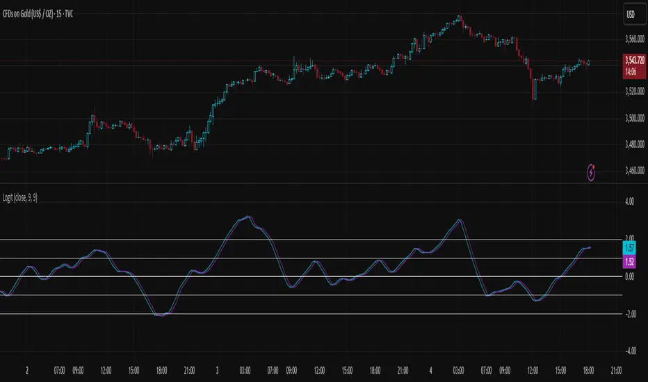
RB — Rejection Blocks (Price Structure)This indicator detects and visualizes Rejection Blocks (RBs) using pure price action logic.
A bullish RB occurs when a down candle forms a lower low than both its neighbors. A bearish RB occurs when an up candle forms a higher high than both its neighbors.
Validated RBs are displayed as boxes, optional lines, or labels. Blocks are automatically removed when invalidated (price closes through them), keeping the chart uncluttered and focused.
How to use
• Apply on any timeframe, from intraday to higher timeframes.
• Watch how price reacts when revisiting RB zones.
• Treat these zones as contextual areas, not entry signals.
• Combine with your own trading methods for confirmation.
Originality
Unlike generic support/resistance tools, this indicator isolates a specific structural pattern (rejection blocks) and renders it visually on the chart. This selective focus allows traders to study structural reactions with more clarity and precision.
⚠️ Disclaimer: This is not a trading system or a signal provider. It is a visual analysis tool designed for structural and educational purposes.

BTC/USD 3-Min Binary Prediction [v7.2 EN]BTC/USD 3-Minute Binary Prediction Indicator v7.2 - Complete Guide
Overview
This is an advanced technical analysis indicator designed for Bitcoin/USD binary options trading with 3-minute expiration times. The system aims for an 83% win rate by combining multiple analysis layers and pattern recognition.
How It Works
Core Prediction Logic
- Timeframe: Predicts whether BTC price will be ±$25 higher (HIGH) or lower (LOW) after 3 minutes
- Entry Signals: Generates HIGH/LOW signals when confidence exceeds threshold (default 75%)
- Verification: Automatically tracks and displays win/loss statistics in real-time
5-Layer Filter System
The indicator uses a sophisticated scoring system (0-100 points):
1. Trend Filter (25 points) - Analyzes EMA alignments and price momentum
2. Leading Indicators (25 points) - RSI and MACD divergence analysis
3. Volume Confirmation (20 points) - Detects unusual volume patterns
4. Support/Resistance (15 points) - Identifies key price levels
5. Momentum Alignment (15 points) - Measures acceleration and deceleration
Pattern Recognition
Automatically detects and visualizes:
- Double Tops/Bottoms - Reversal patterns
- Triangles - Ascending, descending, symmetrical
- Channels - Trending price channels
- Candlestick Patterns - Engulfing, hammer, hanging man
Multi-Timeframe Analysis
- Uses 1-minute and 5-minute data for confirmation
- Aligns multiple timeframes for higher probability trades
- Monitors trend consistency across timeframes
Key Features
Display Panels
1. Statistics Panel (Top Right)
- Overall win rate percentage
- Hourly performance (wins/losses)
- Daily performance
- Current system status
2. Analysis Panel (Left Side)
- Market trend analysis
- RSI status (overbought/oversold)
- Volume conditions
- Filter scores for each component
- Final HIGH/LOW/WAIT decision
Visual Signals
- Green Triangle (↑) = HIGH prediction
- Red Triangle (↓) = LOW prediction
- Yellow Background = Entry opportunity
- Blue Background = Waiting for result
Configuration Options
Basic Settings
- Range Width: Target price movement (default $50 = ±$25)
- Min Confidence: Minimum confidence to enter (default 75%)
- Max Daily Trades: Risk management limit (default 5)
Filters (Can be toggled on/off)
- Trend Filter
- Volume Confirmation
- Support/Resistance Filter
- Momentum Alignment
Display Options
- Show/hide signals, statistics, analysis
- Minimal Mode for cleaner charts
- EMA line visibility
Important Risk Warnings
Binary Options Trading Risks:
1. High Risk Product - Binary options are extremely risky and banned in many countries
2. Not Investment Advice - This tool is for educational/analytical purposes only
3. No Guaranteed Returns - Past performance doesn't predict future results
4. Capital at Risk - You can lose your entire investment in seconds
Technical Limitations:
- Requires stable internet connection
- Performance varies with market conditions
- High volatility can reduce accuracy
- Not suitable for news events or low liquidity periods
Best Practices
1. Paper Trade First - Test thoroughly on demo accounts
2. Risk Management - Never risk more than 1-2% per trade
3. Market Conditions - Works best in normal volatility conditions
4. Avoid Major Events - Don't trade during major news releases
5. Monitor Performance - Track your actual results vs displayed statistics
Setup Instructions
1. Add to TradingView chart (BTC/USD preferred)
2. Use 30-second or 1-minute chart timeframe
3. Adjust settings based on your risk tolerance
4. Monitor F-Score (should be >65 for entries)
5. Wait for clear HIGH/LOW signals with high confidence
Alert Configuration
The indicator provides three alert types:
- HIGH Signal alerts
- LOW Signal alerts
- General entry opportunity alerts
Legal Disclaimer
Binary options trading may not be legal in your jurisdiction. Many countries including the USA, Canada, and EU nations have restrictions or outright bans on binary options. Always check local regulations and consult with financial advisors before trading.
Remember: This is a technical analysis tool, not a money-printing machine. Successful trading requires discipline, risk management, and continuous learning. The displayed statistics are historical and don't guarantee future performance.
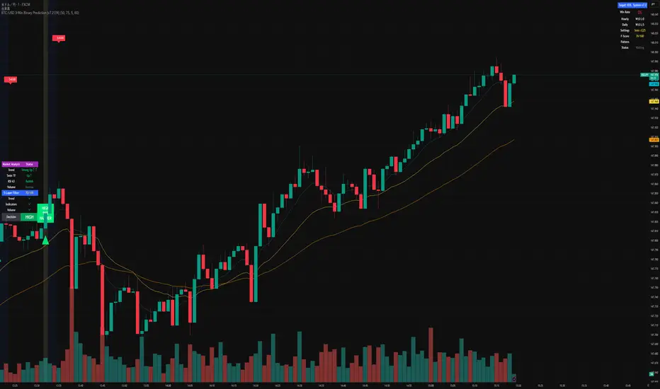
🏆 AI Gold Master IndicatorsAI Gold Master Indicators - Technical Overview
Core Purpose: Advanced Pine Script indicator that analyzes 20 technical indicators simultaneously for XAUUSD (Gold) trading, generating automated buy/sell signals through a sophisticated scoring system.
Key Features
📊 Multi-Indicator Analysis
Processes 20 indicators: RSI, MACD, Bollinger Bands, EMA crossovers, Stochastic, Williams %R, CCI, ATR, Volume, ADX, Parabolic SAR, Ichimoku, MFI, ROC, Fibonacci retracements, Support/Resistance, Candlestick patterns, MA Ribbon, VWAP, Market Structure, and Cloud MA
Each indicator generates BUY (🟢), SELL (🔴), or NEUTRAL (⚪) signals
⚖️ Dual Scoring Systems
Weighted System: Each indicator has configurable weights (10-200 points, total 1000), with higher weights for critical indicators like RSI (150) and MACD (150)
Simple Count System: Basic counting of BUY vs SELL signals across all indicators
🎯 Signal Generation
Configurable thresholds for both systems (weighted score threshold: 400-600 recommended)
Dynamic risk management with ATR-based TP/SL levels
Signal strength filtering to reduce false positives
📈 Advanced Configuration
Customizable thresholds for all 20 indicators (RSI levels, Stochastic bounds, Williams %R zones, etc.)
Dynamic weight bonuses that adapt to dominant market trends
Risk management with configurable TP1/TP2 multipliers and stop losses
🎛️ Visual Interface
Real-time master table displaying all indicators, their values, weights, and current signals
Visual trading signals (triangles) with detailed labels
Optional TP/SL lines and performance statistics
💡 Optimization Features
Gold-specific parameter tuning
Trend analysis with configurable lookback periods
Volume spike detection and volatility analysis
Multi-timeframe compatibility (15m, 1H, 4H recommended)
The system combines traditional technical analysis with modern weighting algorithms to provide comprehensive market analysis specifically optimized for gold trading.
Ragazzi è una meraviglia, pronto all uso, già configurato provatelo divertitevi e fate tanti soldoni poi magari una piccola donazione spontanea sarebbe molto gradita visto il tempo, risorse e gli insulti della moglie che mi diceva che perdevo tempo, fatemi sapere se vi piace.
nel codice troverete una descrizione del funzionamento se vi vengono in mente delle idee per migliorarlo contattatemi troverete i mie contatti in tabella un saluto.

Dual Channel System [Alpha Extract]A sophisticated trend-following and reversal detection system that constructs dynamic support and resistance channels using volatility-adjusted ATR calculations and EMA smoothing for optimal market structure analysis. Utilizing advanced dual-zone methodology with step-like boundary evolution, this indicator delivers institutional-grade channel analysis that adapts to varying volatility conditions while providing high-probability entry and exit signals through breakthrough and rejection detection with comprehensive visual mapping and alert integration.
🔶 Advanced Channel Construction
Implements dual-zone architecture using recent price extremes as foundation points, applying EMA smoothing to reduce noise and ATR multipliers for volatility-responsive channel widths. The system creates resistance channels from highest highs and support channels from lowest lows with asymmetric multiplier ratios for optimal market reaction zones.
// Core Channel Calculation Framework
ATR = ta.atr(14)
// Resistance Channel Construction
Resistance_Basis = ta.ema(ta.highest(high, lookback), lookback)
Resistance_Upper = Resistance_Basis + (ATR * resistance_mult)
Resistance_Lower = Resistance_Basis - (ATR * resistance_mult * 0.3)
// Support Channel Construction
Support_Basis = ta.ema(ta.lowest(low, lookback), lookback)
Support_Upper = Support_Basis + (ATR * support_mult * 0.4)
Support_Lower = Support_Basis - (ATR * support_mult)
// Smoothing Application
Smoothed_Resistance_Upper = ta.ema(Resistance_Upper, smooth_periods)
Smoothed_Support_Lower = ta.ema(Support_Lower, smooth_periods)
🔶 Volatility-Adaptive Zone Framework
Features dynamic ATR-based width adjustment that expands channels during high-volatility periods and contracts during consolidation phases, preventing false signals while maintaining sensitivity to genuine breakouts. The asymmetric multiplier system optimizes zone boundaries for realistic market behavior patterns.
// Dynamic Volatility Adjustment
Channel_Width_Resistance = ATR * resistance_mult
Channel_Width_Support = ATR * support_mult
// Asymmetric Zone Optimization
Resistance_Zone = Resistance_Basis ± (ATR_Multiplied * )
Support_Zone = Support_Basis ± (ATR_Multiplied * )
🔶 Step-Like Boundary Evolution
Creates horizontal step boundaries that update on smoothed bound changes, providing visual history of evolving support and resistance levels with performance-optimized array management limited to 50 historical levels for clean chart presentation and efficient processing.
🔶 Comprehensive Signal Detection
Generates break and bounce signals through sophisticated crossover analysis, monitoring price interaction with smoothed channel boundaries for high-probability entry and exit identification. The system distinguishes between breakthrough continuation and rejection reversal patterns with precision timing.
🔶 Enhanced Visual Architecture
Provides translucent zone fills with gradient intensity scaling, step-like historical boundaries, and dynamic background highlighting that activates upon zone entry. The visual system uses institutional color coding with red resistance zones and green support zones for intuitive
market structure interpretation.
🔶 Intelligent Zone Management
Implements automatic zone relevance filtering, displaying channels only when price proximity warrants analysis attention. The system maintains optimal performance through smart array management and historical level tracking with configurable lookback periods for various market conditions.
🔶 Multi-Dimensional Analysis Framework
Combines trend continuation analysis through breakthrough patterns with reversal detection via rejection signals, providing comprehensive market structure assessment suitable for both trending and ranging market conditions with volatility-normalized accuracy.
🔶 Advanced Alert Integration
Features comprehensive notification system covering breakouts, breakdowns, rejections, and bounces with customizable alert conditions. The system enables precise position management through real-time notifications of critical channel interaction events and zone boundary violations.
🔶 Performance Optimization
Utilizes efficient EMA smoothing algorithms with configurable periods for noise reduction while maintaining responsiveness to genuine market structure changes. The system includes automatic historical level cleanup and performance-optimized visual rendering for smooth operation across all timeframes.
Why Choose Dual Channel System ?
This indicator delivers sophisticated channel-based market analysis through volatility-adaptive ATR calculations and intelligent zone construction methodology. By combining dynamic support and resistance detection with advanced signal generation and comprehensive visual mapping, it provides institutional-grade channel analysis suitable for cryptocurrency, forex, and equity markets. The system's ability to adapt to varying volatility conditions while maintaining signal accuracy makes it essential for traders seeking systematic approaches to breakout trading, zone reversals, and trend continuation analysis with clearly defined risk parameters and comprehensive alert integration. Also to note, this indicator is best suited for the 1D timeframe.
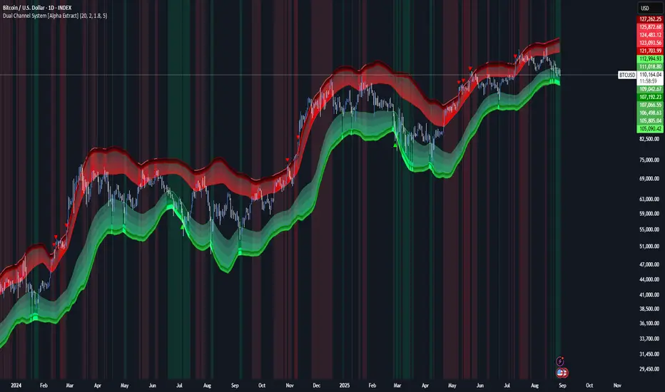
VWAP Price ChannelVWAP Price Channel cuts the crust off of a traditional price channel (Donchian Channel) by anchoring VWAPs at the highs and lows. By doing this, the flat levels, characteristic of traditional Donchian Channels, are no more!
Author's Note: This indicator is formed with no inherent use, and serves solely as a thought experiment.
> Concept
I would be hesitant to call this a "predictive" indicator, however the behavior of it would suggest it could be considered at least partially predictive
Essentially, the Anchored VWAPs creates something from otherwise nothing.
While the DC upper or lower values are staying flat, the VWAPs improvise based on price and volume to project a level that may be a better representation of where future highs or lows may settle.
Visually, this looks like we have cut off the corners of the Donchian Channel.
Note: Notice how we are calculating values before the corners are realized.
> Implementation
While this is only a concept indicator, The specific application I've gone with for this, is a sort of supertrend-ish display (A Trend Flipping Trailing Stop Loss).
The script uses basic logic to create a trend direction, and then displays the Anchored VWAPs as a form of trailing stop loss.
While "In Trend", the script fills in the area between the VWAP and Price in the direction of trend.
When new highs or lows are made while in trend, the opposite VWAP will start to generate at the new highs or lows. These happen on every new high or low, so they are not indicating the trend shift, but could be interpreted as breakout levels for the current trend direction in order for continuation.
Note: All values are drawn live, but when using higher timeframes, there is a natural calculation discrepancy when using live data vs. historical.
> Technicals
In this script, I'm simply detecting new highs or lows from the DC and using those as the anchor frequency on the built-in VWAP function.
So each time a new high or low is made based on DC, the VWAP function re-anchors to the high or low of the candle.
Past that, I have implemented some logic in order to account for a common occurrence I faced during development.
Frequently, the price would outpace the anchored VWAP, so we would end up with the VWAP being further from price than the actual DC upper or lower.
Due to this, what I have ended up with was a third value which, rather than switching between raw VWAP values and DC values, it adjusts the value based on the change in the VWAP value.
This can be simply thought of as a "Start + Change" type of setup.
By doing this, I can use the change values from the actual anchored VWAP, and under normal conditions, this will also be the true VWAP value.
However, situationally, I am able to update the start value which we're applying the VWAP change to.
In other words, when these situations happen, the VWAP change is added to the new (closer to price) DC value.
The specific trend logic being used is nothing fancy at all, we are simply checking if a new high or low is created and setting the trend in that direction.
This is in line with some traditional DC Strategies.
To those who made it here,
Just remember:
The chart may be ugly, but it's the fastest analysis of the data you can get.
Nicer displays often come at the hidden cost of latency.
You have to shoot your shot to make it.
Choose 2: Fast, Clean, Useful
Enjoy!

Reverse RSI Signals [AlgoAlpha]🟠 OVERVIEW
This script introduces the Reverse RSI Signals system, an original approach that inverts traditional RSI values back into price levels and then overlays them directly on the chart as dynamic bands. Instead of showing RSI in a subwindow, the script calculates the exact price thresholds that correspond to common RSI levels (30/70/50) and displays them as upper, lower, and midline bands. These are further enhanced with an adaptive Supertrend filter and divergence detection, allowing traders to see overbought/oversold zones translated into actionable price ranges and trend signals. The script combines concepts of RSI inversion, volatility envelopes, and divergence tracking to provide a context-driven tool for spotting reversals and regime shifts.
🟠 CONCEPTS
The script relies on inverting RSI math: by solving for the price that would yield a given RSI level, it generates real chart levels tied to oscillator conditions. These RSI-derived price bands act like support/resistance, adapting each bar as RSI changes. On top of this, a Supertrend built around the RSI midline introduces directional bias, switching regimes when the midline is breached. Regular bullish and bearish divergences are detected by comparing RSI pivots against price pivots, highlighting early reversal conditions. This layered approach means the indicator is not just RSI on price but a hybrid of oscillator translation, volatility-tracking midline envelopes, and divergence analysis.
🟠 FEATURES
Inverted RSI bands: upper (70), lower (30), and midline (50), smoothed with EMA for noise reduction.
Supertrend overlay on the RSI midline to confirm regime direction (bullish or bearish).
Gradient-filled zones between outer and inner RSI bands to visualize proximity and exhaustion.
Non-repainting bullish and bearish divergence markers plotted directly on chart highs/lows.
🟠 USAGE
Apply the indicator to any chart and use the plotted RSI price bands as adaptive support/resistance. The midline defines equilibrium, while upper and lower bands represent classic RSI thresholds translated into real price action. In bullish regimes (green candles), long trades are stronger when price approaches or bounces from the lower band; in bearish regimes (red candles), shorts are favored near the upper band. Divergence markers (▲ for bullish, ▼ for bearish) flag potential reversal points early. Traders can combine the band proximity, divergence alerts, and Supertrend context to time entries, exits, or to refine ongoing trend trades. Adjust smoothing and Supertrend ATR settings to match the volatility of the instrument being analyzed.

[blackcat] L3 Improved Dual Ehlers BPF for Volatility DetectionOVERVIEW
This script implements an advanced L3 Improved Dual Ehlers Bandpass Filter (BPF) for volatility detection, combining both L1 and L2 calculation methods to create a comprehensive trading signal. The script leverages John Ehlers' sophisticated digital signal processing techniques to identify market cycles and extract meaningful trading signals from price action. By combining multiple cycle detection methods and filtering approaches, it provides traders with a powerful tool for identifying trend changes, momentum shifts, and potential reversal points across various market conditions and timeframes. The L3 approach uniquely combines the outputs of both L1 (01 range) and L2 (-11 range) methods, creating a signal that ranges from -1~2 and provides enhanced sensitivity to market dynamics.
FEATURES
🔄 Dual Calculation Methods: Choose between L1 (01 range), L2 (-11 range), or combine both for L3 signal (-1~2 range) to match your trading style
📊 Multiple Cycle Detection: Seven different dominant cycle calculation methods including HoDyDC (Hilbert Transform Dominant Cycle), PhAcDC (Phase Accumulation Dominant Cycle), DuDiDC (Duane Dominant Cycle), CycPer (Cycle Period), BPZC (Bandpass Zero Crossing), AutoPer (Autocorrelation Period), and DFTDC (Discrete Fourier Transform Dominant Cycle)
🎛️ Flexible Mixing Options: Six sophisticated mixing methods including weighted averaging, simple sum, difference extraction, dominant-only, subdominant-only, and adaptive mixing that adjusts based on signal strength
🌊 Bandpass Filtering: Precise bandwidth control for both dominant and subdominant filters, allowing fine-tuning of frequency response characteristics
📈 Advanced Divergence Detection: Robust algorithm for identifying bullish and bearish divergences with customizable lookback periods and range constraints
🎨 Comprehensive Visualization: Extensive customization options for all signals, colors, plot styles, and display elements
🔔 Comprehensive Alert System: Built-in alerts for divergence signals, zero line crosses, and various market conditions
📊 Real-time Cycle Information: Optional display of dominant and subdominant cycle periods for educational purposes
🔄 Adaptive Signal Processing: Dynamic adjustment of parameters based on market conditions and volatility
🎯 Multiple Signal Outputs: Simultaneous generation of L1, L2, and L3 signals for different trading strategies
HOW TO USE
Select Calculation Method: Choose between "l1" (01 range), "l2" (-11 range), or "both" (L3, -1~2 range) in the Calculation Method settings based on your preferred signal characteristics
Configure Cycle Detection: Select your preferred Dominant Cycle Method from the seven available options and adjust the Cycle Part parameter (0.1-0.9) to fine-tune cycle sensitivity
Set Subdominant Parameters: Configure the subdominant cycle either as a ratio of the dominant cycle or as a fixed period, depending on your analysis approach
Adjust Filter Bandwidth: Fine-tune the bandwidth settings for both dominant and subdominant filters (0.1-1.0) to control the frequency response and signal smoothing
Choose Mixing Method: Select how to combine the filters - weighted averaging for balance, sum for maximum sensitivity, difference for trend isolation, or adaptive mixing for dynamic response
Configure Smoothing: Select from SMA, EMA, or HMA smoothing methods with adjustable length (1-20 bars) to reduce noise in the final signal
Customize Visualization: Enable/disable individual plots, divergence detection, zero line, fill areas, and customize all colors to match your chart preferences
Set Divergence Parameters: Configure lookback ranges (5-60 bars) for divergence detection to match your trading timeframe and style
Monitor Signals: Watch for crosses above/below zero line and divergence patterns, paying attention to signal strength and consistency
Set Up Alerts: Configure alerts for divergence signals, zero line crosses, and other market conditions to stay informed of trading opportunities
LIMITATIONS
The script requires the dc_ta library from blackcat1402 for several advanced cycle calculation methods (HoDyDC, PhAcDC, DuDiDC, CycPer, BPZC, AutoPer, DFTDC)
L1 method operates in 01 range while L2 method uses -11 range, requiring different interpretation approaches
Combined L3 signal ranges from -1~2 when both methods are selected, creating unique signal characteristics that traders must adapt to
Divergence detection accuracy depends on proper lookback period settings and market volatility conditions
Performance may be impacted with very long lookback ranges (>60 bars) or when multiple plots are simultaneously enabled
The script is designed for non-overlay use and may not display correctly on certain chart types or with conflicting indicators
Adaptive mixing method requires careful threshold tuning to avoid excessive signal fluctuation
Cycle detection algorithms may produce unreliable results during low volatility or highly choppy market conditions
The script assumes regular price data and may not perform optimally with irregular or gapped price sequences
NOTES
The script implements advanced mathematical calculations including bandpass filters, Hilbert transforms, and various cycle detection algorithms developed by John Ehlers
For optimal results, experiment with different cycle detection methods and bandwidth settings across various market conditions and timeframes
The adaptive mixing method automatically adjusts weights based on signal strength, providing dynamic response to changing market conditions
Divergence detection works best when the "Plot Divergence" option is enabled and when combined with other technical analysis tools
Zero line crosses can indicate potential trend changes or momentum shifts, especially when confirmed by volume or other indicators
The script includes commented code for cycle information display that can be enabled if you want to monitor cycle periods in real-time
Different calculation methods may perform better in different market environments - L1 tends to be smoother while L2 is more sensitive
The subdominant cycle helps filter out noise and provides additional confirmation for signals generated by the dominant cycle
Bandwidth settings control the filter's frequency response - lower values provide more smoothing while higher values increase sensitivity
Mixing methods offer different approaches to combining signals - weighted averaging is generally most reliable for most trading applications
THANKS
Special thanks to John Ehlers for his pioneering work in cycle analysis and digital signal processing for financial markets. This script implements and significantly improves upon his bandpass filter methodology, incorporating multiple advanced techniques from his extensive body of work. Also heartfelt thanks to blackcat1402 for the dc_ta library that provides essential cycle calculation methods and for maintaining such a valuable resource for the Pine Script community. Additional appreciation to the TradingView platform for providing the tools and environment that make sophisticated technical analysis accessible to traders worldwide. This script represents a collaborative effort in advancing the field of algorithmic trading and technical analysis.
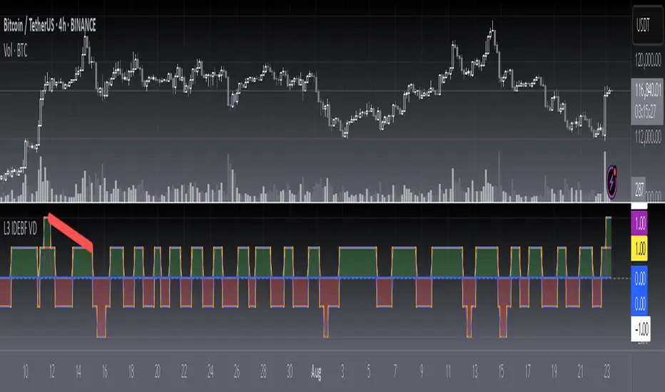
[blackcat] L1 Value Trend IndicatorOVERVIEW
The L1 Value Trend Indicator is a sophisticated technical analysis tool designed for TradingView users seeking advanced market trend identification and trading signals. This comprehensive indicator combines multiple analytical techniques to provide traders with a holistic view of market dynamics, helping identify potential entry and exit points through various signal mechanisms. 📈 It features a main Value Trend line along with a lagged version, golden cross and dead cross signals, and multiple technical indicators including RSI, Williams %R, Stochastic %K/D, and Relative Strength calculations. The indicator also includes reference levels for support and resistance analysis, making it a versatile tool for both short-term and long-term trading strategies. ✅
FEATURES
📈 Primary Value Trend Line: Calculates a smoothed value trend using a combination of SMA and custom smoothing techniques
🔍 Value Trend Lag: Implements a lagged version of the main trend line for cross-over analysis
🚀 Golden Cross & Dead Cross Signals: Identifies buy/sell opportunities when the main trend line crosses its lagged version
💸 Multi-Indicator Integration: Combines multiple technical analysis tools for comprehensive market view
📊 RSI Calculations: Includes 6-period, 7-period, and 13-period RSI calculations for momentum analysis
📈 Williams %R: Provides overbought/oversold conditions using the Williams %R formula
📉 Stochastic Oscillator: Implements both Stochastic %K and %D calculations for momentum confirmation
📋 Relative Strength: Calculates relative strength based on highest highs and current price
✅ Visual Labels: Displays BUY and SELL labels on chart when crossover conditions are met
📣 Alert Conditions: Provides automated alert conditions for golden cross and dead cross events
📌 Reference Levels: Plots entry (25) and exit (75) reference lines for support/resistance analysis
HOW TO USE
Copy the Script: Copy the complete Pine Script code from the original file
Open TradingView: Navigate to TradingView website or application
Access Pine Editor: Go to the Pine Script editor (usually found in the chart toolbar)
Paste Code: Paste the copied script into the editor
Save Script: Save the script with a descriptive name like " L1 Value Trend Indicator"
Select Chart: Choose the chart where you want to apply the indicator
Add Indicator: Apply the indicator to your chart
Configure Parameters: Adjust input parameters to customize behavior
Monitor Signals: Watch for golden cross (BUY) and dead cross (SELL) signals
Use Reference Levels: Monitor entry (25) and exit (75) lines for support/resistance levels
LIMITATIONS
⚠️ Potential Repainting: The script may repaint due to lookahead bias in some calculations
📉 Lookahead Bias: Some calculations may reference future values, potentially causing repainting issues
🔄 Parameter Sensitivity: Results may vary significantly with different parameter settings
📉 Computational Complexity: May impact chart performance with heavy calculations on large datasets
📊 Resource Usage: Requires significant processing power for multiple indicator calculations
🔄 Data Sensitivity: Results may be affected by data quality and market conditions
NOTES
📈 Signal Timing: Cross-over signals may lag behind actual price movements
📉 Parameter Optimization: Optimal parameters may vary by market conditions and asset type
📋 Market Conditions: Performance may vary significantly across different market environments
📈 Multi-Indicator: Combine signals with other technical indicators for confirmation
📉 Timeframe Analysis: Use multiple timeframes for enhanced signal accuracy
📋 Volume Analysis: Incorporate volume data for additional confirmation
📈 Strategy Integration: Consider using this indicator as part of a broader trading strategy
📉 Risk Management: Use signals as part of a comprehensive risk management approach
📋 Backtesting: Test parameter combinations with historical data before live trading
THANKS
🙏 Original Creator: blackcat1402 creates the L1 Value Trend Indicator
📚 Community Contributions: Recognition to TradingView community for continuous improvements and contributions
📈 Collaborative Development: Appreciation for collaborative efforts in enhancing technical analysis tools
📉 TradingView Community: Special thanks to TradingView community members for their ongoing support and feedback
📋 Educational Resources: Recognition of educational resources that helped in understanding technical analysis principles
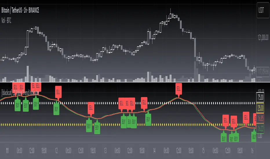
T-Virus Sentiment [hapharmonic]🧬 T-Virus Sentiment: Visualize the Market's DNA
Remember the iconic T-Virus vial from the first Resident Evil? That powerful, swirling helix of potential has always fascinated me. It sparked an idea: what if we could visualize the market's underlying health in a similar way? What if we could capture the "genetic code" of market sentiment and contain it within a dynamic, 3D indicator? This project is the result of that idea, brought to life with Pine Script.
The indicator's main goal is to measure the strength and direction of market sentiment by analyzing the "genetic code" of price action through a variety of trusted indicators. The result is displayed as a liquid level within a DNA helix, a bubble density representing buying pressure, and a T-Virus mascot that reflects the overall mood.
🧐 Core Concept: How It Works
The primary output of the indicator is the "Active %" gauge you see on the right side of the vial. This percentage represents the overall sentiment score, calculated as an average from 7 different technical analysis tools. Each tool is analyzed on every bar and assigned a score from 1 (strong bearish pressure) to 5 (strong bullish potential).
In this indicator, we re-imagine market dynamics through the lens of a viral outbreak. A strong bear market is like a virus taking hold, pulling all technical signals down into a state of weakness. Conversely, a powerful bull market is like an antiviral serum ; positive signals rise and spread toward the top of the vial, indicating that the system is being injected with strength.
This is not just another line on a chart. It's a comprehensive sentiment dashboard designed to give an immediate, at-a-glance understanding of the confluence between 7 classic technical indicators. The incredible 3D model of the vial itself was inspired by a design concept found here .
⚛️ The 4 Core Elements of T-Virus Sentiment
These four elements work in harmony to give a complete, multi-faceted picture of market sentiment. Each component tells a different part of the story.
The Virus Mascot: An instant emotional cue. This character provides the quickest possible read on the overall market mood, combining sentiment with volume pressure.
The Antiviral Serum Level: The main quantitative output. This is the liquid level in the DNA helix and the percentage gauge on the right, representing the average sentiment score from all 7 indicators.
Buy Pressure & Bubble Density: This visualizes volume flow. The density of bubbles represents the intensity of accumulation (buying) versus distribution (selling). It's the "power" behind the move.
The Signal Distribution: This shows the confluence (or dispersion) of sentiment. Are all signals bullish and clustered at the top, or are they scattered, indicating a conflicted market? The position of the indicator labels is crucial, as each is assigned to one of five distinct zones:
Base Bottom: The market is at its weakest. Signals here suggest strong bearish control and distribution.
Lower Zone: The market is still bearish, but signals may be showing early signs of accumulation or bottoming.
Neutral Core (Center): A state of balance or sideways consolidation. The market is waiting for a new direction.
Upper Zone: Bullish momentum is becoming clear. Signals are strengthening and showing bullish control.
Top Cap: The market is "heating up" with strong bullish sentiment, potentially nearing overbought conditions.
🐂🐻 The Virus Mascot: The At-a-Glance Indicator
This character acts as a shortcut to confirm market health. It combines the sentiment score with volume, preventing false confidence in a low-volume rally.
Its state is determined by a dual-check: the overall "Antiviral Serum Level" and the "Buy Pressure" must both be above 50%.
Green & Smiling: The 'all clear' signal. This means that not only is the overall technical sentiment bullish, but it's also being supported by real buying pressure. This is a sign of a healthy bull market.
Red & Angry: A warning sign. This appears if either the sentiment is weak, or a bullish sentiment is not being confirmed by buying volume. The latter could indicate a potential "bull trap" or an exhaustive move.
This mascot can be disabled from the settings page under "Virus Mascot Styling" if a cleaner look is preferred.
🫧 Bubble Density: Gauging Buy vs. Sell Pressure
The bubbles visualize the battle between buyers and sellers. There are two modes to control how this is calculated:
Mode 1: Visible Range (The 'Big Picture' View)
This default mode is best for getting a broad, contextual understanding of the current session. It dynamically analyzes the volume of every single candlestick currently visible on the screen to calculate the buy/sell pressure ratio. It answers the question: "Over the entire period I'm looking at, who is in control?" As you zoom in or out, the calculation adapts.
Mode 2: Custom Lookback (The 'Precision' View)
This mode is for traders who need to analyze short-term pressure. You can define a fixed number of recent bars to analyze, which is perfect for scalping or understanding the volume dynamics leading into a key level. It answers the question: "What is happening right now ?" In the example above, a lookback of 2 focuses only on the most recent action, clearly showing intense, immediate selling pressure (few bubbles) and a corresponding drop in the sentiment score to 29%.
ℹ️ Interactive Tooltips: Dive Deeper
We believe in transparency, not 'black box' indicators. This feature transforms the indicator from a visual aid into an active learning tool.
Simply hover the mouse over any indicator label (like EMA, OBV, etc.) to get a detailed tooltip. It will explain the specific data points and thresholds that signal met to be placed in its current zone. This helps build trust in the signals and allows users to fine-tune the indicator settings to better match their own trading style.
🎯 The Scoring Logic Breakdown
The "Antiviral Serum Level" gauge is the average score from 7 technical analysis tools. Each is graded on a 5-point scale (1=Strong Bearish to 5=Strong Bullish). Here’s a detailed, transparent look at how each "gene" is evaluated:
Relative Strength Index (RSI)
Measures momentum and overbought/oversold conditions.
Group 1 (Strong Bearish): RSI > 80 (Extreme Overbought)
Group 2 (Bearish): 70 < RSI ≤ 80 (Overbought)
Group 3 (Neutral): 30 ≤ RSI ≤ 70
Group 4 (Bullish): 20 ≤ RSI < 30 (Oversold)
Group 5 (Strong Bullish): RSI < 20 (Extreme Oversold)
Exponential Moving Averages (EMA)
Evaluates the trend's strength and structure based on the alignment of multiple EMAs (9, 21, 50, 100, 200, 250).
Group 1 (Strong Bearish): A perfect bearish sequence (9 < 21 < 50 < ...)
Group 2 (Bearish Transition): Early signs of a potential reversal (e.g., 9 > 21 but still below 50)
Group 3 (Neutral / Mixed): MAs are intertwined or showing a partial bullish sequence.
Group 4 (Bullish): A strong bullish sequence is forming (e.g., 9 > 21 > 50 > 100)
Group 5 (Strong Bullish): A perfect bullish sequence (9 > 21 > 50 > 100 > 200 > 250)
Moving Average Convergence Divergence (MACD)
Analyzes the relationship between two moving averages to gauge momentum.
Group 1 (Strong Bearish): MACD & Histogram are negative and momentum is falling.
Group 2 (Weakening Bearish): MACD is negative but the histogram is rising or positive.
Group 3 (Neutral / Crossover): A crossover event is occurring near the zero line.
Group 4 (Bullish): MACD & Histogram are positive.
Group 5 (Strong Bullish): MACD & Histogram are positive, rising strongly, and accelerating.
Average Directional Index (ADX)
Measures trend strength, not direction. The score is based on both ADX value and the dominance of DI+ vs DI-.
Group 1 (Bearish / No Trend): ADX < 20 and DI- is dominant.
Group 2 (Developing Bearish Trend): 20 ≤ ADX < 25 and DI- is dominant.
Group 3 (Neutral / Indecision): Trend is weak or DI+ and DI- are nearly equal.
Group 4 (Developing Bullish Trend): 25 ≤ ADX ≤ 40 and DI+ is dominant.
Group 5 (Strong Bullish Trend): ADX > 40 and DI+ is dominant.
Ichimoku Cloud (IKH)
A comprehensive indicator that defines support/resistance, momentum, and trend direction.
Group 1 (Strong Bearish): Price is below the Kumo, Tenkan < Kijun, and Chikou is below price.
Group 2 (Bearish): Price is inside or below the Kumo, with mixed secondary signals.
Group 3 (Neutral / Ranging): Price is inside the Kumo, often with a Tenkan/Kijun cross.
Group 4 (Bullish): Price is above the Kumo with strong primary signals.
Group 5 (Strong Bullish): All signals are aligned bullishly: price above Kumo, bullish Tenkan/Kijun cross, bullish future Kumo, and Chikou above price.
Bollinger Bands (BB)
Measures volatility and relative price levels.
Group 1 (Strong Bearish): Price is below the lower band.
Group 2 (Bearish Territory): Price is between the lower band and the basis line.
Group 3 (Neutral): Price is hovering around the basis line.
Group 4 (Bullish Territory): Price is between the basis line and the upper band.
Group 5 (Strong Bullish): Price is above the upper band.
On-Balance Volume (OBV)
Uses volume flow to predict price changes. The score is based on OBV's trend and its position relative to its moving average.
Group 1 (Strong Bearish): OBV is below its MA and falling.
Group 2 (Weakening Bearish): OBV is below its MA but showing signs of rising.
Group 3 (Neutral): OBV is very close to its MA.
Group 4 (Bullish): OBV is above its MA and rising.
Group 5 (Strong Bullish): OBV is above its MA, rising strongly, and showing signs of a volume spike.
🧭 How to Use the T-Virus Sentiment Indicator
IMPORTANT: This indicator is a sentiment dashboard , not a direct buy/sell signal generator. Its strength lies in showing confluence and providing a quick, holistic view of the market's technical health.
Confirmation Tool: Use the "Active %" gauge to confirm a trade setup from your primary strategy. For example, if you see a bullish chart pattern, a high and rising sentiment score can add confidence to your trade.
Momentum & Trend Gauge: A consistently high score (e.g., > 75%) suggests strong, established bullish momentum. A consistently low score (< 25%) suggests strong bearish control. A score hovering around 50% often indicates a ranging or indecisive market.
Divergence & Warning System: Pay attention to divergences. If the price is making new highs but the sentiment score is failing to follow or is actively decreasing, it could be an early warning sign that the underlying momentum is weakening.
⚙️ Settings & Customization
The indicator is highly customizable to fit any trading style.
Position & Anchor: Control where the vial appears on the chart.
Styling (Vial, Helix, etc.): Nearly every visual element can be color-customized.
Signals: This is where the real power is. All underlying indicator parameters (RSI length, MACD settings, etc.) can be fine-tuned to match a personal strategy. The text labels can also be disabled if the chart feels cluttered.
Enjoy visualizing the market's DNA with the T-Virus Sentiment indicator

RSI Dynamic Bands█ OVERVIEW
The "RSI Dynamic Bands" indicator is a variant of the Relative Strength Index (RSI) oscillator that brings its signals directly onto the price chart. It displays dynamic bands around the price, adjusted based on RSI levels, enabling easy identification of potential overbought or oversold conditions. The indicator also integrates a multi-timeframe RSI table, facilitating the analysis of trend strength across different timeframes.
█ CONCEPTS
The "RSI Dynamic Bands" indicator is designed to simplify the interpretation of price levels in the context of support and resistance zones, which can be correlated with other technical indicators and RSI values. Since the price itself does not display RSI values, a table showing RSI for four selected timeframes has been added, allowing traders to quickly assess trend strength across different time intervals. The most effective approach is to combine the indicator with other technical analysis tools, such as Fibonacci levels or pivot points, to confirm signals when the price approaches the bands and RSI values indicate a potential reversal.
Band Calculation
The bands are calculated based on the current closing price and RSI values, incorporating dynamic scaling to better adapt to market conditions. The formulas for the bands are as follows:
• Upper Band: close + (rsiUpper - rsi) * scaleFactor, where rsiUpper is the upper RSI level (default: 70), and scaleFactor accounts for market volatility.
• Lower Band: close + (rsiLower - rsi) * scaleFactor, where rsiLower is the lower RSI level (default: 30).
• Midline: The arithmetic average of the upper and lower bands: (upperBand + lowerBand) / 2.
Why Scaling? Without scaling, the bands would be chaotic and jagged, making them difficult to interpret. Scaling smooths the bands, making them wider during periods of high volatility and narrower during consolidation, better reflecting potential support and resistance levels.
Indicator Features
• Dynamic Price Bands: The bands adapt to market conditions, facilitating the identification of key price levels.
• Multi-Timeframe RSI Table: Displays RSI values for four selected timeframes (default: 15m, 1h, 4h, Daily), enabling comparison of trend strength across different perspectives.
• Style Customization: Users can adjust band colors, line thickness, and toggle the visibility of bands, fills, and the table.
How to Set Up the Indicator
1 — Add the "RSI Dynamic Bands" indicator to your TradingView chart.
2 — Configure parameters in the settings, such as RSI length, upper/lower levels, and scaling multiplier, to match your trading style.
3 — Enable or disable the display of bands, fills, or the RSI table based on your needs.
4 — Adjust band and table colors in the input section and line thickness in the "Style" section to better align the indicator with your chart.
█ OTHER SECTIONS
FEATURES
• RSI Length: The period for calculating RSI (default: 14).
• RSI Levels: Thresholds for overbought (default: 70) and oversold (default: 30).
• Scaling Multiplier: Adjusts bands based on market volatility (default: 0.15).
• Table Timeframes: Select four timeframes for the RSI table (default: 15m, 1h, 4h, Daily).
• Style Options: Customize band colors, fills, table, and line thickness.
HOW TO USE
Add the indicator to your chart, configure the parameters, and observe price interactions with the bands to identify potential entry and exit points. The RSI table allows you to compare RSI values across different timeframes, aiding in trading decisions. The most effective approach is to combine the indicator with other technical analysis tools, such as Fibonacci levels or pivot points, to confirm signals when the price approaches the bands and RSI values indicate a potential reversal.
Trading Strategies:
• Scalping: Use lower timeframes (e.g., 5m, 15m) in the RSI table to quickly identify short-term lows and highs. Wait for the price to approach the lower band in the RSI oversold zone, with RSI on lower timeframes starting to rise, and other tools, such as Fibonacci levels (e.g., 38.2%) or pivot points, confirming support.
• Medium-Term Trading: Focus on 1h and 4h timeframes. Look for confirmation of a low on a lower timeframe (e.g., 1h), where RSI indicates oversold conditions or starts rising, then check if RSI on a higher timeframe (e.g., 4h) confirms the trend. Confirmation from other tools, such as a Fibonacci level (e.g., 50%) or pivot point near the bands, strengthens the signal.
• Long-Term Trading: Use Daily and higher timeframes (e.g., Weekly). Wait for all relevant timeframes to confirm a low (e.g., RSI near oversold and price at the lower band), with lower timeframes (e.g., 4h) showing rising RSI. Other tools, such as Fibonacci levels (e.g., 61.8%) or pivot points near the bands, can further confirm a trend reversal signal.

The Barking Rat LiteMomentum & FVG Reversion Strategy
The Barking Rat Lite is a disciplined, short-term mean-reversion strategy that combines RSI momentum filtering, EMA bands, and Fair Value Gap (FVG) detection to identify short-term reversal points. Designed for practical use on volatile markets, it focuses on precise entries and ATR-based take profit management to balance opportunity and risk.
Core Concept
This strategy seeks potential reversals when short-term price action shows exhaustion outside an EMA band, confirmed by momentum and FVG signals:
EMA Bands:
Parameters used: A 20-period EMA (fast) and 100-period EMA (slow).
Why chosen:
- The 20 EMA is sensitive to short-term moves and reflects immediate momentum.
- The 100 EMA provides a slower, structural anchor.
When price trades outside both bands, it often signals overextension relative to both short-term and medium-term trends.
Application in strategy:
- Long entries are only considered when price dips below both EMAs, identifying potential undervaluation.
- Short entries are only considered when price rises above both EMAs, identifying potential overvaluation.
This dual-band filter avoids counter-trend signals that would occur if only a single EMA was used, making entries more selective..
Fair Value Gap Detection (FVG):
Parameters used: The script checks for dislocations using a 12-bar lookback (i.e. comparing current highs/lows with values 12 candles back).
Why chosen:
- A 12-bar displacement highlights significant inefficiencies in price structure while filtering out micro-gaps that appear every few bars in high-volatility markets.
- By aligning FVG signals with candle direction (bullish = close > open, bearish = close < open), the strategy avoids random gaps and instead targets ones that suggest exhaustion.
Application in strategy:
- Bullish FVGs form when earlier lows sit above current highs, hinting at downward over-extension.
- Bearish FVGs form when earlier highs sit below current lows, hinting at upward over-extension.
This gives the strategy a structural filter beyond simple oscillators, ensuring signals have price-dislocation context.
RSI Momentum Filter:
Parameters used: 14-period RSI with thresholds of 80 (overbought) and 20 (oversold).
Why chosen:
- RSI(14) is a widely recognized momentum measure that balances responsiveness with stability.
- The thresholds are intentionally extreme (80/20 vs. the more common 70/30), so the strategy only engages at genuine exhaustion points rather than frequent minor corrections.
Application in strategy:
- Longs trigger when RSI < 20, suggesting oversold exhaustion.
- Shorts trigger when RSI > 80, suggesting overbought exhaustion.
This ensures entries are not just technically valid but also backed by momentum extremes, raising conviction.
ATR-Based Take Profit:
Parameters used: 14-period ATR, with a default multiplier of 4.
Why chosen:
- ATR(14) reflects the prevailing volatility environment without reacting too much to outliers.
- A multiplier of 4 is a pragmatic compromise: wide enough to let trades breathe in volatile conditions, but tight enough to enforce disciplined exits before mean reversion fades.
Application in strategy:
- At entry, a fixed target is set = Entry Price ± (ATR × 4).
- This target scales automatically with volatility: narrower in calm periods, wider in explosive markets.
By avoiding discretionary exits, the system maintains rule-based discipline.
Visual Signals on Chart
Blue “▲” below candle: Potential long entry
Orange/Yellow “▼” above candle: Potential short entry
Green “✔️”: Trade closed at ATR take profit
Blue (20 EMA) & Orange (100 EMA) lines: Dynamic channel reference
⚙️Strategy report properties
Position size: 25% equity per trade
Initial capital: 10,000.00 USDT
Pyramiding: 10 entries per direction
Slippage: 2 ticks
Commission: 0.055% per side
Backtest timeframe: 1-minute
Backtest instrument: HYPEUSDT
Backtesting range: Jul 28, 2025 — Aug 17, 2025
Note on Sample Size:
You’ll notice the report displays fewer than the ideal 100 trades in the strategy report above. This is intentional. The goal of the script is to isolate high-quality, short-term reversal opportunities while filtering out low-conviction setups. This means that the Barking Rat Lite strategy is very selective, filtering out over 90% of market noise. The brief timeframe shown in the strategy report here illustrates its filtering logic over a short window — not its full capabilities. As a result, even on lower timeframes like the 1-minute chart, signals are deliberately sparse — each one must pass all criteria before triggering.
For a larger dataset:
Once the strategy is applied to your chart, users are encouraged to expand the lookback range or apply the strategy to other volatile pairs to view a full sample.
💡Why 25% Equity Per Trade?
While it's always best to size positions based on personal risk tolerance, we defaulted to 25% equity per trade in the backtesting data — and here’s why:
Backtests using this sizing show manageable drawdowns even under volatile periods.
The strategy generates a sizeable number of trades, reducing reliance on a single outcome.
Combined with conservative filters, the 25% setting offers a balance between aggression and control.
Users are strongly encouraged to customize this to suit their risk profile.
What makes Barking Rat Lite valuable
Combines multiple layers of confirmation: EMA bands + FVG + RSI
Adaptive to volatility: ATR-based exits scale with market conditions
Clear, actionable visuals: Easy to monitor and manage trades

NAS100 Component Sentiment Scanner# NAS100 Component Sentiment Scanner
## 🎯 Overview
The NAS100 Component Sentiment Scanner analyzes the top-weighted stocks in the NASDAQ-100 index to provide real-time bullish/bearish sentiment signals that can help predict NAS100 price movements. This indicator combines multiple technical analysis methods to give traders a comprehensive view of underlying market sentiment.
## 📊 How It Works
The indicator calculates sentiment scores for major NASDAQ-100 components (AAPL, MSFT, NVDA, GOOGL, AMZN, META, TSLA, AVGO, COST, NFLX) using:
- **RSI Analysis**: Identifies overbought/oversold conditions
- **Moving Average Trends**: Compares fast vs slow MA positioning
- **Volume Confirmation**: Validates moves with volume thresholds
- **Price Momentum**: Analyzes recent price direction
- **Market Cap Weighting**: Uses actual NASDAQ-100 weightings for accuracy
## 🚀 Key Features
### Real-Time Sentiment Analysis
- Weighted composite score based on individual stock analysis
- Color-coded sentiment line (Green = Bullish, Red = Bearish)
- Dynamic background coloring for strong signals
### Interactive Data Table
- Shows individual stock scores and signals
- Bullish/Bearish stock count summary
- Customizable position and size
### Smart Signal System
- **Bullish Signals**: Green triangle up when sentiment crosses threshold
- **Bearish Signals**: Red triangle down when sentiment falls below threshold
- **Alert Conditions**: Automatic notifications for signal changes
## ⚙️ Customization Options
### Technical Analysis Settings
- **RSI Period**: Adjust lookback period (default: 14)
- **RSI Levels**: Set overbought/oversold thresholds
- **Moving Averages**: Configure fast/slow MA periods
- **Volume Threshold**: Set volume confirmation multiplier
### Signal Thresholds
- **Bullish/Bearish Levels**: Customize trigger points
- **Strong Signal Levels**: Set extreme sentiment thresholds
- Fine-tune sensitivity to market conditions
### Display Options
- **Toggle Table**: Show/hide sentiment data table
- **Table Position**: 6 position options (Top/Bottom/Middle + Left/Right)
- **Table Size**: Choose from Tiny, Small, Normal, or Large
- **Background Colors**: Enable/disable signal backgrounds
- **Signal Arrows**: Show/hide buy/sell indicators
### Stock Selection
- **Individual Control**: Enable/disable any of the 10 major stocks
- **Dynamic Weighting**: Automatically adjusts calculations based on selected stocks
- **Flexible Analysis**: Focus on specific sectors or market leaders
## 📈 How to Use
### 1. Basic Setup
1. Add the indicator to your NAS100 chart
2. Default settings work well for most traders
3. Observe the sentiment line and signals
### 2. Signal Interpretation
- **Score > 30**: Bullish bias for NAS100
- **Score > 50**: Strong bullish signal
- **Score -30 to 30**: Neutral/consolidation
- **Score < -30**: Bearish bias for NAS100
- **Score < -50**: Strong bearish signal
### 3. Trading Strategies
**Trend Following:**
- Buy NAS100 when bullish signals appear
- Sell/short when bearish signals trigger
- Use background colors for quick visual confirmation
**Divergence Trading:**
- Watch for sentiment/price divergences
- Strong sentiment with weak NAS100 price = potential breakout
- Weak sentiment with strong NAS100 price = potential reversal
**Consensus Trading:**
- Monitor bullish/bearish stock counts in table
- 8+ stocks aligned = strong directional bias
- Mixed signals = wait for clearer consensus
### 4. Advanced Usage
- Combine with your existing NAS100 trading strategy
- Use multiple timeframes for confirmation
- Adjust thresholds based on market volatility
- Focus on specific stocks by disabling others
## 🔔 Alert Setup
The indicator includes built-in alert conditions:
1. Go to TradingView Alerts
2. Select "NAS100 Component Sentiment Scanner"
3. Choose from available alert types:
- NAS100 Bullish Signal
- NAS100 Bearish Signal
- Strong Bullish Consensus
- Strong Bearish Consensus
## 💡 Pro Tips
### Optimization
- **High Volatility**: Increase signal thresholds (±40, ±60)
- **Low Volatility**: Decrease thresholds (±20, ±40)
- **Day Trading**: Use smaller table, focus on real-time signals
- **Swing Trading**: Enable background colors, larger thresholds
### Best Practices
- Don't use as a standalone system - combine with price action
- Check individual stock table for context
- Monitor during market open for most reliable signals
- Consider earnings seasons for individual stock impacts
### Market Conditions
- **Trending Markets**: Higher accuracy, use with trend following
- **Ranging Markets**: Watch for false signals, increase thresholds
- **News Events**: Individual stock news can skew sentiment temporarily
## 🎨 Visual Guide
- **Green Line Above Zero**: Bullish sentiment building
- **Red Line Below Zero**: Bearish sentiment building
- **Background Color Changes**: Strong signal confirmation
- **Triangle Arrows**: Entry/exit signal points
- **Table Colors**: Quick sentiment overview
## ⚠️ Important Notes
- This indicator analyzes component stocks, not NAS100 directly
- Market cap weightings approximate real NASDAQ-100 weightings
- Sentiment can change rapidly during volatile periods
- Always use proper risk management
- Combine with other technical analysis tools
## 🔧 Troubleshooting
- **No signals**: Check if thresholds are too extreme
- **Too many signals**: Increase threshold sensitivity
- **Table not showing**: Ensure "Show Sentiment Table" is enabled
- **Missing stocks**: Verify individual stock toggles in settings
---
**Suitable for**: Day traders, swing traders, NAS100 specialists, index traders
**Best Timeframes**: 5min, 15min, 1H, 4H
**Market Sessions**: US market hours for highest accuracy

Ray Dalio's All Weather Strategy - Portfolio CalculatorTHE ALL WEATHER STRATEGY INDICATOR: A GUIDE TO RAY DALIO'S LEGENDARY PORTFOLIO APPROACH
Introduction: The Genesis of Financial Resilience
In the sprawling corridors of Bridgewater Associates, the world's largest hedge fund managing over 150 billion dollars in assets, Ray Dalio conceived what would become one of the most influential investment strategies of the modern era. The All Weather Strategy, born from decades of market observation and rigorous backtesting, represents a paradigm shift from traditional portfolio construction methods that have dominated Wall Street since Harry Markowitz's seminal work on Modern Portfolio Theory in 1952.
Unlike conventional approaches that chase returns through market timing or stock picking, the All Weather Strategy embraces a fundamental truth that has humbled countless investors throughout history: nobody can consistently predict the future direction of markets. Instead of fighting this uncertainty, Dalio's approach harnesses it, creating a portfolio designed to perform reasonably well across all economic environments, hence the evocative name "All Weather."
The strategy emerged from Bridgewater's extensive research into economic cycles and asset class behavior, culminating in what Dalio describes as "the Holy Grail of investing" in his bestselling book "Principles" (Dalio, 2017). This Holy Grail isn't about achieving spectacular returns, but rather about achieving consistent, risk-adjusted returns that compound steadily over time, much like the tortoise defeating the hare in Aesop's timeless fable.
HISTORICAL DEVELOPMENT AND EVOLUTION
The All Weather Strategy's origins trace back to the tumultuous economic periods of the 1970s and 1980s, when traditional portfolio construction methods proved inadequate for navigating simultaneous inflation and recession. Raymond Thomas Dalio, born in 1949 in Queens, New York, founded Bridgewater Associates from his Manhattan apartment in 1975, initially focusing on currency and fixed-income consulting for corporate clients.
Dalio's early experiences during the 1970s stagflation period profoundly shaped his investment philosophy. Unlike many of his contemporaries who viewed inflation and deflation as opposing forces, Dalio recognized that both conditions could coexist with either economic growth or contraction, creating four distinct economic environments rather than the traditional two-factor models that dominated academic finance.
The conceptual breakthrough came in the late 1980s when Dalio began systematically analyzing asset class performance across different economic regimes. Working with a small team of researchers, Bridgewater developed sophisticated models that decomposed economic conditions into growth and inflation components, then mapped historical asset class returns against these regimes. This research revealed that traditional portfolio construction, heavily weighted toward stocks and bonds, left investors vulnerable to specific economic scenarios.
The formal All Weather Strategy emerged in 1996 when Bridgewater was approached by a wealthy family seeking a portfolio that could protect their wealth across various economic conditions without requiring active management or market timing. Unlike Bridgewater's flagship Pure Alpha fund, which relied on active trading and leverage, the All Weather approach needed to be completely passive and unleveraged while still providing adequate diversification.
Dalio and his team spent months developing and testing various allocation schemes, ultimately settling on the 30/40/15/7.5/7.5 framework that balances risk contributions rather than dollar amounts. This approach was revolutionary because it focused on risk budgeting—ensuring that no single asset class dominated the portfolio's risk profile—rather than the traditional approach of equal dollar allocations or market-cap weighting.
The strategy's first institutional implementation began in 1996 with a family office client, followed by gradual expansion to other wealthy families and eventually institutional investors. By 2005, Bridgewater was managing over $15 billion in All Weather assets, making it one of the largest systematic strategy implementations in institutional investing.
The 2008 financial crisis provided the ultimate test of the All Weather methodology. While the S&P 500 declined by 37% and many hedge funds suffered double-digit losses, the All Weather strategy generated positive returns, validating Dalio's risk-balancing approach. This performance during extreme market stress attracted significant institutional attention, leading to rapid asset growth in subsequent years.
The strategy's theoretical foundations evolved throughout the 2000s as Bridgewater's research team, led by co-chief investment officers Greg Jensen and Bob Prince, refined the economic framework and incorporated insights from behavioral economics and complexity theory. Their research, published in numerous institutional white papers, demonstrated that traditional portfolio optimization methods consistently underperformed simpler risk-balanced approaches across various time periods and market conditions.
Academic validation came through partnerships with leading business schools and collaboration with prominent economists. The strategy's risk parity principles influenced an entire generation of institutional investors, leading to the creation of numerous risk parity funds managing hundreds of billions in aggregate assets.
In recent years, the democratization of sophisticated financial tools has made All Weather-style investing accessible to individual investors through ETFs and systematic platforms. The availability of high-quality, low-cost ETFs covering each required asset class has eliminated many of the barriers that previously limited sophisticated portfolio construction to institutional investors.
The development of advanced portfolio management software and platforms like TradingView has further democratized access to institutional-quality analytics and implementation tools. The All Weather Strategy Indicator represents the culmination of this trend, providing individual investors with capabilities that previously required teams of portfolio managers and risk analysts.
Understanding the Four Economic Seasons
The All Weather Strategy's theoretical foundation rests on Dalio's observation that all economic environments can be characterized by two primary variables: economic growth and inflation. These variables create four distinct "economic seasons," each favoring different asset classes. Rising growth benefits stocks and commodities, while falling growth favors bonds. Rising inflation helps commodities and inflation-protected securities, while falling inflation benefits nominal bonds and stocks.
This framework, detailed extensively in Bridgewater's research papers from the 1990s, suggests that by holding assets that perform well in each economic season, an investor can create a portfolio that remains resilient regardless of which season unfolds. The elegance lies not in predicting which season will occur, but in being prepared for all of them simultaneously.
Academic research supports this multi-environment approach. Ang and Bekaert (2002) demonstrated that regime changes in economic conditions significantly impact asset returns, while Fama and French (2004) showed that different asset classes exhibit varying sensitivities to economic factors. The All Weather Strategy essentially operationalizes these academic insights into a practical investment framework.
The Original All Weather Allocation: Simplicity Masquerading as Sophistication
The core All Weather portfolio, as implemented by Bridgewater for institutional clients and later adapted for retail investors, maintains a deceptively simple static allocation: 30% stocks, 40% long-term bonds, 15% intermediate-term bonds, 7.5% commodities, and 7.5% Treasury Inflation-Protected Securities (TIPS). This allocation may appear arbitrary to the uninitiated, but each percentage reflects careful consideration of historical volatilities, correlations, and economic sensitivities.
The 30% stock allocation provides growth exposure while limiting the portfolio's overall volatility. Stocks historically deliver superior long-term returns but with significant volatility, as evidenced by the Standard & Poor's 500 Index's average annual return of approximately 10% since 1926, accompanied by standard deviation exceeding 15% (Ibbotson Associates, 2023). By limiting stock exposure to 30%, the portfolio captures much of the equity risk premium while avoiding excessive volatility.
The combined 55% allocation to bonds (40% long-term plus 15% intermediate-term) serves as the portfolio's stabilizing force. Long-term bonds provide substantial interest rate sensitivity, performing well during economic slowdowns when central banks reduce rates. Intermediate-term bonds offer a balance between interest rate sensitivity and reduced duration risk. This bond-heavy allocation reflects Dalio's insight that bonds typically exhibit lower volatility than stocks while providing essential diversification benefits.
The 7.5% commodities allocation addresses inflation protection, as commodity prices typically rise during inflationary periods. Historical analysis by Bodie and Rosansky (1980) demonstrated that commodities provide meaningful diversification benefits and inflation hedging capabilities, though with considerable volatility. The relatively small allocation reflects commodities' high volatility and mixed long-term returns.
Finally, the 7.5% TIPS allocation provides explicit inflation protection through government-backed securities whose principal and interest payments adjust with inflation. Introduced by the U.S. Treasury in 1997, TIPS have proven effective inflation hedges, though they underperform nominal bonds during deflationary periods (Campbell & Viceira, 2001).
Historical Performance: The Evidence Speaks
Analyzing the All Weather Strategy's historical performance reveals both its strengths and limitations. Using monthly return data from 1970 to 2023, spanning over five decades of varying economic conditions, the strategy has delivered compelling risk-adjusted returns while experiencing lower volatility than traditional stock-heavy portfolios.
During this period, the All Weather allocation generated an average annual return of approximately 8.2%, compared to 10.5% for the S&P 500 Index. However, the strategy's annual volatility measured just 9.1%, substantially lower than the S&P 500's 15.8% volatility. This translated to a Sharpe ratio of 0.67 for the All Weather Strategy versus 0.54 for the S&P 500, indicating superior risk-adjusted performance.
More impressively, the strategy's maximum drawdown over this period was 12.3%, occurring during the 2008 financial crisis, compared to the S&P 500's maximum drawdown of 50.9% during the same period. This drawdown mitigation proves crucial for long-term wealth building, as Stein and DeMuth (2003) demonstrated that avoiding large losses significantly impacts compound returns over time.
The strategy performed particularly well during periods of economic stress. During the 1970s stagflation, when stocks and bonds both struggled, the All Weather portfolio's commodity and TIPS allocations provided essential protection. Similarly, during the 2000-2002 dot-com crash and the 2008 financial crisis, the portfolio's bond-heavy allocation cushioned losses while maintaining positive returns in several years when stocks declined significantly.
However, the strategy underperformed during sustained bull markets, particularly the 1990s technology boom and the 2010s post-financial crisis recovery. This underperformance reflects the strategy's conservative nature and diversified approach, which sacrifices potential upside for downside protection. As Dalio frequently emphasizes, the All Weather Strategy prioritizes "not losing money" over "making a lot of money."
Implementing the All Weather Strategy: A Practical Guide
The All Weather Strategy Indicator transforms Dalio's institutional-grade approach into an accessible tool for individual investors. The indicator provides real-time portfolio tracking, rebalancing signals, and performance analytics, eliminating much of the complexity traditionally associated with implementing sophisticated allocation strategies.
To begin implementation, investors must first determine their investable capital. As detailed analysis reveals, the All Weather Strategy requires meaningful capital to implement effectively due to transaction costs, minimum investment requirements, and the need for precise allocations across five different asset classes.
For portfolios below $50,000, the strategy becomes challenging to implement efficiently. Transaction costs consume a disproportionate share of returns, while the inability to purchase fractional shares creates allocation drift. Consider an investor with $25,000 attempting to allocate 7.5% to commodities through the iPath Bloomberg Commodity Index ETF (DJP), currently trading around $25 per share. This allocation targets $1,875, enough for only 75 shares, creating immediate tracking error.
At $50,000, implementation becomes feasible but not optimal. The 30% stock allocation ($15,000) purchases approximately 37 shares of the SPDR S&P 500 ETF (SPY) at current prices around $400 per share. The 40% long-term bond allocation ($20,000) buys 200 shares of the iShares 20+ Year Treasury Bond ETF (TLT) at approximately $100 per share. While workable, these allocations leave significant cash drag and rebalancing challenges.
The optimal minimum for individual implementation appears to be $100,000. At this level, each allocation becomes substantial enough for precise implementation while keeping transaction costs below 0.4% annually. The $30,000 stock allocation, $40,000 long-term bond allocation, $15,000 intermediate-term bond allocation, $7,500 commodity allocation, and $7,500 TIPS allocation each provide sufficient size for effective management.
For investors with $250,000 or more, the strategy implementation approaches institutional quality. Allocation precision improves, transaction costs decline as a percentage of assets, and rebalancing becomes highly efficient. These larger portfolios can also consider adding complexity through international diversification or alternative implementations.
The indicator recommends quarterly rebalancing to balance transaction costs with allocation discipline. Monthly rebalancing increases costs without substantial benefits for most investors, while annual rebalancing allows excessive drift that can meaningfully impact performance. Quarterly rebalancing, typically on the first trading day of each quarter, provides an optimal balance.
Understanding the Indicator's Functionality
The All Weather Strategy Indicator operates as a comprehensive portfolio management system, providing multiple analytical layers that professional money managers typically reserve for institutional clients. This sophisticated tool transforms Ray Dalio's institutional-grade strategy into an accessible platform for individual investors, offering features that rival professional portfolio management software.
The indicator's core architecture consists of several interconnected modules that work seamlessly together to provide complete portfolio oversight. At its foundation lies a real-time portfolio simulation engine that tracks the exact value of each ETF position based on current market prices, eliminating the need for manual calculations or external spreadsheets.
DETAILED INDICATOR COMPONENTS AND FUNCTIONS
Portfolio Configuration Module
The portfolio setup begins with the Portfolio Configuration section, which establishes the fundamental parameters for strategy implementation. The Portfolio Capital input accepts values from $1,000 to $10,000,000, accommodating everyone from beginning investors to institutional clients. This input directly drives all subsequent calculations, determining exact share quantities and portfolio values throughout the implementation period.
The Portfolio Start Date function allows users to specify when they began implementing the All Weather Strategy, creating a clear demarcation point for performance tracking. This feature proves essential for investors who want to track their actual implementation against theoretical performance, providing realistic assessment of strategy effectiveness including timing differences and implementation costs.
Rebalancing Frequency settings offer two options: Monthly and Quarterly. While monthly rebalancing provides more precise allocation control, quarterly rebalancing typically proves more cost-effective for most investors due to reduced transaction costs. The indicator automatically detects the first trading day of each period, ensuring rebalancing occurs at optimal times regardless of weekends, holidays, or market closures.
The Rebalancing Threshold parameter, adjustable from 0.5% to 10%, determines when allocation drift triggers rebalancing recommendations. Conservative settings like 1-2% maintain tight allocation control but increase trading frequency, while wider thresholds like 3-5% reduce trading costs but allow greater allocation drift. This flexibility accommodates different risk tolerances and cost structures.
Visual Display System
The Show All Weather Calculator toggle controls the main dashboard visibility, allowing users to focus on chart visualization when detailed metrics aren't needed. When enabled, this comprehensive dashboard displays current portfolio value, individual ETF allocations, target versus actual weights, rebalancing status, and performance metrics in a professionally formatted table.
Economic Environment Display provides context about current market conditions based on growth and inflation indicators. While simplified compared to Bridgewater's sophisticated regime detection, this feature helps users understand which economic "season" currently prevails and which asset classes should theoretically benefit.
Rebalancing Signals illuminate when portfolio drift exceeds user-defined thresholds, highlighting specific ETFs that require adjustment. These signals use color coding to indicate urgency: green for balanced allocations, yellow for moderate drift, and red for significant deviations requiring immediate attention.
Advanced Label System
The rebalancing label system represents one of the indicator's most innovative features, providing three distinct detail levels to accommodate different user needs and experience levels. The "None" setting displays simple symbols marking portfolio start and rebalancing events without cluttering the chart with text. This minimal approach suits experienced investors who understand the implications of each symbol.
"Basic" label mode shows essential information including portfolio values at each rebalancing point, enabling quick assessment of strategy performance over time. These labels display "START $X" for portfolio initiation and "RBL $Y" for rebalancing events, providing clear performance tracking without overwhelming detail.
"Detailed" labels provide comprehensive trading instructions including exact buy and sell quantities for each ETF. These labels might display "RBL $125,000 BUY 15 SPY SELL 25 TLT BUY 8 IEF NO TRADES DJP SELL 12 SCHP" providing complete implementation guidance. This feature essentially transforms the indicator into a personal portfolio manager, eliminating guesswork about exact trades required.
Professional Color Themes
Eight professionally designed color themes adapt the indicator's appearance to different aesthetic preferences and market analysis styles. The "Gold" theme reflects traditional wealth management aesthetics, while "EdgeTools" provides modern professional appearance. "Behavioral" uses psychologically informed colors that reinforce disciplined decision-making, while "Quant" employs high-contrast combinations favored by quantitative analysts.
"Ocean," "Fire," "Matrix," and "Arctic" themes provide distinctive visual identities for traders who prefer unique chart aesthetics. Each theme automatically adjusts for dark or light mode optimization, ensuring optimal readability across different TradingView configurations.
Real-Time Portfolio Tracking
The portfolio simulation engine continuously tracks five separate ETF positions: SPY for stocks, TLT for long-term bonds, IEF for intermediate-term bonds, DJP for commodities, and SCHP for TIPS. Each position's value updates in real-time based on current market prices, providing instant feedback about portfolio performance and allocation drift.
Current share calculations determine exact holdings based on the most recent rebalancing, while target shares reflect optimal allocation based on current portfolio value. Trade calculations show precisely how many shares to buy or sell during rebalancing, eliminating manual calculations and potential errors.
Performance Analytics Suite
The indicator's performance measurement capabilities rival professional portfolio analysis software. Sharpe ratio calculations incorporate current risk-free rates obtained from Treasury yield data, providing accurate risk-adjusted performance assessment. Volatility measurements use rolling periods to capture changing market conditions while maintaining statistical significance.
Portfolio return calculations track both absolute and relative performance, comparing the All Weather implementation against individual asset classes and benchmark indices. These metrics update continuously, providing real-time assessment of strategy effectiveness and implementation quality.
Data Quality Monitoring
Sophisticated data quality checks ensure reliable indicator operation across different market conditions and potential data interruptions. The system monitors all five ETF price feeds plus economic data sources, providing quality scores that alert users to potential data issues that might affect calculations.
When data quality degrades, the indicator automatically switches to fallback values or alternative data sources, maintaining functionality during temporary market data interruptions. This robust design ensures consistent operation even during volatile market conditions when data feeds occasionally experience disruptions.
Risk Management and Behavioral Considerations
Despite its sophisticated design, the All Weather Strategy faces behavioral challenges that have derailed countless well-intentioned investment plans. The strategy's conservative nature means it will underperform growth stocks during bull markets, potentially by substantial margins. Maintaining discipline during these periods requires understanding that the strategy optimizes for risk-adjusted returns over absolute returns.
Behavioral finance research by Kahneman and Tversky (1979) demonstrates that investors feel losses approximately twice as intensely as equivalent gains. This loss aversion creates powerful psychological pressure to abandon defensive strategies during bull markets when aggressive portfolios appear more attractive. The All Weather Strategy's bond-heavy allocation will seem overly conservative when technology stocks double in value, as occurred repeatedly during the 2010s.
Conversely, the strategy's defensive characteristics provide psychological comfort during market stress. When stocks crash 30-50%, as they periodically do, the All Weather portfolio's modest losses feel manageable rather than catastrophic. This emotional stability enables investors to maintain their investment discipline when others capitulate, often at the worst possible times.
Rebalancing discipline presents another behavioral challenge. Selling winners to buy losers contradicts natural human tendencies but remains essential for the strategy's success. When stocks have outperformed bonds for several quarters, rebalancing requires selling high-performing stock positions to purchase seemingly stagnant bond positions. This action feels counterintuitive but captures the strategy's systematic approach to risk management.
Tax considerations add complexity for taxable accounts. Frequent rebalancing generates taxable events that can erode after-tax returns, particularly for high-income investors facing elevated capital gains rates. Tax-advantaged accounts like 401(k)s and IRAs provide ideal vehicles for All Weather implementation, eliminating tax friction from rebalancing activities.
Capital Requirements and Cost Analysis
Comprehensive cost analysis reveals the capital requirements for effective All Weather implementation. Annual expenses include management fees for each ETF, transaction costs from rebalancing, and bid-ask spreads from trading less liquid securities.
ETF expense ratios vary significantly across asset classes. The SPDR S&P 500 ETF charges 0.09% annually, while the iShares 20+ Year Treasury Bond ETF charges 0.20%. The iShares 7-10 Year Treasury Bond ETF charges 0.15%, the Schwab US TIPS ETF charges 0.05%, and the iPath Bloomberg Commodity Index ETF charges 0.75%. Weighted by the All Weather allocations, total expense ratios average approximately 0.19% annually.
Transaction costs depend heavily on broker selection and account size. Premium brokers like Interactive Brokers charge $1-2 per trade, resulting in $20-40 annually for quarterly rebalancing. Discount brokers may charge higher per-trade fees but offer commission-free ETF trading for selected funds. Zero-commission brokers eliminate explicit trading costs but often impose wider bid-ask spreads that function as hidden fees.
Bid-ask spreads represent the difference between buying and selling prices for each security. Highly liquid ETFs like SPY maintain spreads of 1-2 basis points, while less liquid commodity ETFs may exhibit spreads of 5-10 basis points. These costs accumulate through rebalancing activities, typically totaling 10-15 basis points annually.
For a $100,000 portfolio, total annual costs including expense ratios, transaction fees, and spreads typically range from 0.35% to 0.45%, or $350-450 annually. These costs decline as a percentage of assets as portfolio size increases, reaching approximately 0.25% for portfolios exceeding $250,000.
Comparing costs to potential benefits reveals the strategy's value proposition. Historical analysis suggests the All Weather approach reduces portfolio volatility by 35-40% compared to stock-heavy allocations while maintaining competitive returns. This volatility reduction provides substantial value during market stress, potentially preventing behavioral mistakes that destroy long-term wealth.
Alternative Implementations and Customizations
While the original All Weather allocation provides an excellent starting point, investors may consider modifications based on personal circumstances, market conditions, or geographic considerations. International diversification represents one potential enhancement, adding exposure to developed and emerging market bonds and equities.
Geographic customization becomes important for non-US investors. European investors might replace US Treasury bonds with German Bunds or broader European government bond indices. Currency hedging decisions add complexity but may reduce volatility for investors whose spending occurs in non-dollar currencies.
Tax-location strategies optimize after-tax returns by placing tax-inefficient assets in tax-advantaged accounts while holding tax-efficient assets in taxable accounts. TIPS and commodity ETFs generate ordinary income taxed at higher rates, making them candidates for retirement account placement. Stock ETFs generate qualified dividends and long-term capital gains taxed at lower rates, making them suitable for taxable accounts.
Some investors prefer implementing the bond allocation through individual Treasury securities rather than ETFs, eliminating management fees while gaining precise maturity control. Treasury auctions provide access to new securities without bid-ask spreads, though this approach requires more sophisticated portfolio management.
Factor-based implementations replace broad market ETFs with factor-tilted alternatives. Value-tilted stock ETFs, quality-focused bond ETFs, or momentum-based commodity indices may enhance returns while maintaining the All Weather framework's diversification benefits. However, these modifications introduce additional complexity and potential tracking error.
Conclusion: Embracing the Long Game
The All Weather Strategy represents more than an investment approach; it embodies a philosophy of financial resilience that prioritizes sustainable wealth building over speculative gains. In an investment landscape increasingly dominated by algorithmic trading, meme stocks, and cryptocurrency volatility, Dalio's methodical approach offers a refreshing alternative grounded in economic theory and historical evidence.
The strategy's greatest strength lies not in its potential for extraordinary returns, but in its capacity to deliver reasonable returns across diverse economic environments while protecting capital during market stress. This characteristic becomes increasingly valuable as investors approach or enter retirement, when portfolio preservation assumes greater importance than aggressive growth.
Implementation requires discipline, adequate capital, and realistic expectations. The strategy will underperform growth-oriented approaches during bull markets while providing superior downside protection during bear markets. Investors must embrace this trade-off consciously, understanding that the strategy optimizes for long-term wealth building rather than short-term performance.
The All Weather Strategy Indicator democratizes access to institutional-quality portfolio management, providing individual investors with tools previously available only to wealthy families and institutions. By automating allocation tracking, rebalancing signals, and performance analysis, the indicator removes much of the complexity that has historically limited sophisticated strategy implementation.
For investors seeking a systematic, evidence-based approach to long-term wealth building, the All Weather Strategy provides a compelling framework. Its emphasis on diversification, risk management, and behavioral discipline aligns with the fundamental principles that have created lasting wealth throughout financial history. While the strategy may not generate headlines or inspire cocktail party conversations, it offers something more valuable: a reliable path toward financial security across all economic seasons.
As Dalio himself notes, "The biggest mistake investors make is to believe that what happened in the recent past is likely to persist, and they design their portfolios accordingly." The All Weather Strategy's enduring appeal lies in its rejection of this recency bias, instead embracing the uncertainty of markets while positioning for success regardless of which economic season unfolds.
STEP-BY-STEP INDICATOR SETUP GUIDE
Setting up the All Weather Strategy Indicator requires careful attention to each configuration parameter to ensure optimal implementation. This comprehensive setup guide walks through every setting and explains its impact on strategy performance.
Initial Setup Process
Begin by adding the indicator to your TradingView chart. Search for "Ray Dalio's All Weather Strategy" in the indicator library and apply it to any chart. The indicator operates independently of the underlying chart symbol, drawing data directly from the five required ETFs regardless of which security appears on the chart.
Portfolio Configuration Settings
Start with the Portfolio Capital input, which drives all subsequent calculations. Enter your exact investable capital, ranging from $1,000 to $10,000,000. This input determines share quantities, trade recommendations, and performance calculations. Conservative recommendations suggest minimum capitals of $50,000 for basic implementation or $100,000 for optimal precision.
Select your Portfolio Start Date carefully, as this establishes the baseline for all performance calculations. Choose the date when you actually began implementing the All Weather Strategy, not when you first learned about it. This date should reflect when you first purchased ETFs according to the target allocation, creating realistic performance tracking.
Choose your Rebalancing Frequency based on your cost structure and precision preferences. Monthly rebalancing provides tighter allocation control but increases transaction costs. Quarterly rebalancing offers the optimal balance for most investors between allocation precision and cost control. The indicator automatically detects appropriate trading days regardless of your selection.
Set the Rebalancing Threshold based on your tolerance for allocation drift and transaction costs. Conservative investors preferring tight control should use 1-2% thresholds, while cost-conscious investors may prefer 3-5% thresholds. Lower thresholds maintain more precise allocations but trigger more frequent trading.
Display Configuration Options
Enable Show All Weather Calculator to display the comprehensive dashboard containing portfolio values, allocations, and performance metrics. This dashboard provides essential information for portfolio management and should remain enabled for most users.
Show Economic Environment displays current economic regime classification based on growth and inflation indicators. While simplified compared to Bridgewater's sophisticated models, this feature provides useful context for understanding current market conditions.
Show Rebalancing Signals highlights when portfolio allocations drift beyond your threshold settings. These signals use color coding to indicate urgency levels, helping prioritize rebalancing activities.
Advanced Label Customization
Configure Show Rebalancing Labels based on your need for chart annotations. These labels mark important portfolio events and can provide valuable historical context, though they may clutter charts during extended time periods.
Select appropriate Label Detail Levels based on your experience and information needs. "None" provides minimal symbols suitable for experienced users. "Basic" shows portfolio values at key events. "Detailed" provides complete trading instructions including exact share quantities for each ETF.
Appearance Customization
Choose Color Themes based on your aesthetic preferences and trading style. "Gold" reflects traditional wealth management appearance, while "EdgeTools" provides modern professional styling. "Behavioral" uses psychologically informed colors that reinforce disciplined decision-making.
Enable Dark Mode Optimization if using TradingView's dark theme for optimal readability and contrast. This setting automatically adjusts all colors and transparency levels for the selected theme.
Set Main Line Width based on your chart resolution and visual preferences. Higher width values provide clearer allocation lines but may overwhelm smaller charts. Most users prefer width settings of 2-3 for optimal visibility.
Troubleshooting Common Setup Issues
If the indicator displays "Data not available" messages, verify that all five ETFs (SPY, TLT, IEF, DJP, SCHP) have valid price data on your selected timeframe. The indicator requires daily data availability for all components.
When rebalancing signals seem inconsistent, check your threshold settings and ensure sufficient time has passed since the last rebalancing event. The indicator only triggers signals on designated rebalancing days (first trading day of each period) when drift exceeds threshold levels.
If labels appear at unexpected chart locations, verify that your chart displays percentage values rather than price values. The indicator forces percentage formatting and 0-40% scaling for optimal allocation visualization.
COMPREHENSIVE BIBLIOGRAPHY AND FURTHER READING
PRIMARY SOURCES AND RAY DALIO WORKS
Dalio, R. (2017). Principles: Life and work. New York: Simon & Schuster.
Dalio, R. (2018). A template for understanding big debt crises. Bridgewater Associates.
Dalio, R. (2021). Principles for dealing with the changing world order: Why nations succeed and fail. New York: Simon & Schuster.
BRIDGEWATER ASSOCIATES RESEARCH PAPERS
Jensen, G., Kertesz, A. & Prince, B. (2010). All Weather strategy: Bridgewater's approach to portfolio construction. Bridgewater Associates Research.
Prince, B. (2011). An in-depth look at the investment logic behind the All Weather strategy. Bridgewater Associates Daily Observations.
Bridgewater Associates. (2015). Risk parity in the context of larger portfolio construction. Institutional Research.
ACADEMIC RESEARCH ON RISK PARITY AND PORTFOLIO CONSTRUCTION
Ang, A. & Bekaert, G. (2002). International asset allocation with regime shifts. The Review of Financial Studies, 15(4), 1137-1187.
Bodie, Z. & Rosansky, V. I. (1980). Risk and return in commodity futures. Financial Analysts Journal, 36(3), 27-39.
Campbell, J. Y. & Viceira, L. M. (2001). Who should buy long-term bonds? American Economic Review, 91(1), 99-127.
Clarke, R., De Silva, H. & Thorley, S. (2013). Risk parity, maximum diversification, and minimum variance: An analytic perspective. Journal of Portfolio Management, 39(3), 39-53.
Fama, E. F. & French, K. R. (2004). The capital asset pricing model: Theory and evidence. Journal of Economic Perspectives, 18(3), 25-46.
BEHAVIORAL FINANCE AND IMPLEMENTATION CHALLENGES
Kahneman, D. & Tversky, A. (1979). Prospect theory: An analysis of decision under risk. Econometrica, 47(2), 263-292.
Thaler, R. H. & Sunstein, C. R. (2008). Nudge: Improving decisions about health, wealth, and happiness. New Haven: Yale University Press.
Montier, J. (2007). Behavioural investing: A practitioner's guide to applying behavioural finance. Chichester: John Wiley & Sons.
MODERN PORTFOLIO THEORY AND QUANTITATIVE METHODS
Markowitz, H. (1952). Portfolio selection. The Journal of Finance, 7(1), 77-91.
Sharpe, W. F. (1964). Capital asset prices: A theory of market equilibrium under conditions of risk. The Journal of Finance, 19(3), 425-442.
Black, F. & Litterman, R. (1992). Global portfolio optimization. Financial Analysts Journal, 48(5), 28-43.
PRACTICAL IMPLEMENTATION AND ETF ANALYSIS
Gastineau, G. L. (2010). The exchange-traded funds manual. 2nd ed. Hoboken: John Wiley & Sons.
Poterba, J. M. & Shoven, J. B. (2002). Exchange-traded funds: A new investment option for taxable investors. American Economic Review, 92(2), 422-427.
Israelsen, C. L. (2005). A refinement to the Sharpe ratio and information ratio. Journal of Asset Management, 5(6), 423-427.
ECONOMIC CYCLE ANALYSIS AND ASSET CLASS RESEARCH
Ilmanen, A. (2011). Expected returns: An investor's guide to harvesting market rewards. Chichester: John Wiley & Sons.
Swensen, D. F. (2009). Pioneering portfolio management: An unconventional approach to institutional investment. Rev. ed. New York: Free Press.
Siegel, J. J. (2014). Stocks for the long run: The definitive guide to financial market returns & long-term investment strategies. 5th ed. New York: McGraw-Hill Education.
RISK MANAGEMENT AND ALTERNATIVE STRATEGIES
Taleb, N. N. (2007). The black swan: The impact of the highly improbable. New York: Random House.
Lowenstein, R. (2000). When genius failed: The rise and fall of Long-Term Capital Management. New York: Random House.
Stein, D. M. & DeMuth, P. (2003). Systematic withdrawal from retirement portfolios: The impact of asset allocation decisions on portfolio longevity. AAII Journal, 25(7), 8-12.
CONTEMPORARY DEVELOPMENTS AND FUTURE DIRECTIONS
Asness, C. S., Frazzini, A. & Pedersen, L. H. (2012). Leverage aversion and risk parity. Financial Analysts Journal, 68(1), 47-59.
Roncalli, T. (2013). Introduction to risk parity and budgeting. Boca Raton: CRC Press.
Ibbotson Associates. (2023). Stocks, bonds, bills, and inflation 2023 yearbook. Chicago: Morningstar.
PERIODICALS AND ONGOING RESEARCH
Journal of Portfolio Management - Quarterly publication featuring cutting-edge research on portfolio construction and risk management
Financial Analysts Journal - Bi-monthly publication of the CFA Institute with practical investment research
Bridgewater Associates Daily Observations - Regular market commentary and research from the creators of the All Weather Strategy
RECOMMENDED READING SEQUENCE
For investors new to the All Weather Strategy, begin with Dalio's "Principles" for philosophical foundation, then proceed to the Bridgewater research papers for technical details. Supplement with Markowitz's original portfolio theory work and behavioral finance literature from Kahneman and Tversky.
Intermediate students should focus on academic papers by Ang & Bekaert on regime shifts, Clarke et al. on risk parity methods, and Ilmanen's comprehensive analysis of expected returns across asset classes.
Advanced practitioners will benefit from Roncalli's technical treatment of risk parity mathematics, Asness et al.'s academic critique of leverage aversion, and ongoing research in the Journal of Portfolio Management.
