Bullish Reversal Bar Strategy [Skyrexio]Overview
Bullish Reversal Bar Strategy leverages the combination of candlestick pattern Bullish Reversal Bar (description in Methodology and Justification of Methodology), Williams Alligator indicator and Williams Fractals to create the high probability setups. Candlestick pattern is used for the entering into trade, while the combination of Williams Alligator and Fractals is used for the trend approximation as close condition. Strategy uses only long trades.
Unique Features
No fixed stop-loss and take profit: Instead of fixed stop-loss level strategy utilizes technical condition obtained by Fractals and Alligator or the candlestick pattern invalidation to identify when current uptrend is likely to be over (more information in "Methodology" and "Justification of Methodology" paragraphs)
Configurable Trading Periods: Users can tailor the strategy to specific market windows, adapting to different market conditions.
Trend Trade Filter: strategy uses Alligator and Fractal combination as high probability trend filter.
Methodology
The strategy opens long trade when the following price met the conditions:
1.Current candle's high shall be below the Williams Alligator's lines (Jaw, Lips, Teeth)(all details in "Justification of Methodology" paragraph)
2.Price shall create the candlestick pattern "Bullish Reversal Bar". Optionally if MFI and AO filters are enabled current candle shall have the decreasing AO and at least one of three recent bars shall have the squat state on the MFI (all details in "Justification of Methodology" paragraph)
3.If price breaks through the high of the candle marked as the "Bullish Reversal Bar" the long trade is open at the price one tick above the candle's high
4.Initial stop loss is placed at the Bullish Reversal Bar's candle's low
5.If price hit the Bullish Reversal Bar's low before hitting the entry price potential trade is cancelled
6.If trade is active and initial stop loss has not been hit, trade is closed when the combination of Alligator and Williams Fractals shall consider current trend change from upward to downward.
Strategy settings
In the inputs window user can setup strategy setting:
Enable MFI (if true trades are filtered using Market Facilitation Index (MFI) condition all details in "Justification of Methodology" paragraph), by default = false)
Enable AO (if true trades are filtered using Awesome Oscillator (AO) condition all details in "Justification of Methodology" paragraph), by default = false)
Justification of Methodology
Let's explore the key concepts of this strategy and understand how they work together. The first and key concept is the Bullish Reversal Bar candlestick pattern. This is just the single bar pattern. The rules are simple:
Candle shall be closed in it's upper half
High of this candle shall be below all three Alligator's lines (Jaw, Lips, Teeth)
Next, let’s discuss the short-term trend filter, which combines the Williams Alligator and Williams Fractals. Williams Alligator
Developed by Bill Williams, the Alligator is a technical indicator that identifies trends and potential market reversals. It consists of three smoothed moving averages:
Jaw (Blue Line): The slowest of the three, based on a 13-period smoothed moving average shifted 8 bars ahead.
Teeth (Red Line): The medium-speed line, derived from an 8-period smoothed moving average shifted 5 bars forward.
Lips (Green Line): The fastest line, calculated using a 5-period smoothed moving average shifted 3 bars forward.
When the lines diverge and align in order, the "Alligator" is "awake," signaling a strong trend. When the lines overlap or intertwine, the "Alligator" is "asleep," indicating a range-bound or sideways market. This indicator helps traders determine when to enter or avoid trades.
Fractals, another tool by Bill Williams, help identify potential reversal points on a price chart. A fractal forms over at least five consecutive bars, with the middle bar showing either:
Up Fractal: Occurs when the middle bar has a higher high than the two preceding and two following bars, suggesting a potential downward reversal.
Down Fractal: Happens when the middle bar shows a lower low than the surrounding two bars, hinting at a possible upward reversal.
Traders often use fractals alongside other indicators to confirm trends or reversals, enhancing decision-making accuracy.
How do these tools work together in this strategy? Let’s consider an example of an uptrend.
When the price breaks above an up fractal, it signals a potential bullish trend. This occurs because the up fractal represents a shift in market behavior, where a temporary high was formed due to selling pressure. If the price revisits this level and breaks through, it suggests the market sentiment has turned bullish.
The breakout must occur above the Alligator’s teeth line to confirm the trend. A breakout below the teeth is considered invalid, and the downtrend might still persist. Conversely, in a downtrend, the same logic applies with down fractals.
How we can use all these indicators in this strategy? This strategy is a counter trend one. Candle's high shall be below all Alligator's lines. During this market stage the bullish reversal bar candlestick pattern shall be printed. This bar during the downtrend is a high probability setup for the potential reversal to the upside: bulls were able to close the price in the upper half of a candle. The breaking of its high is a high probability signal that trend change is confirmed and script opens long trade. If market continues going down and break down the bullish reversal bar's low potential trend change has been invalidated and strategy close long trade.
If market really reversed and started moving to the upside strategy waits for the trend change form the downtrend to the uptrend according to approximation of Alligator and Fractals combination. If this change happens strategy close the trade. This approach helps to stay in the long trade while the uptrend continuation is likely and close it if there is a high probability of the uptrend finish.
Optionally users can enable MFI and AO filters. First of all, let's briefly explain what are these two indicators. The Awesome Oscillator (AO), created by Bill Williams, is a momentum-based indicator that evaluates market momentum by comparing recent price activity to a broader historical context. It assists traders in identifying potential trend reversals and gauging trend strength.
AO = SMA5(Median Price) − SMA34(Median Price)
where:
Median Price = (High + Low) / 2
SMA5 = 5-period Simple Moving Average of the Median Price
SMA 34 = 34-period Simple Moving Average of the Median Price
This indicator is filtering signals in the following way: if current AO bar is decreasing this candle can be interpreted as a bullish reversal bar. This logic is applicable because initially this strategy is a trend reversal, it is searching for the high probability setup against the current trend. Decreasing AO is the additional high probability filter of a downtrend.
Let's briefly look what is MFI. The Market Facilitation Index (MFI) is a technical indicator that measures the price movement per unit of volume, helping traders gauge the efficiency of price movement in relation to trading volume. Here's how you can calculate it:
MFI = (High−Low)/Volume
MFI can be used in combination with volume, so we can divide 4 states. Bill Williams introduced these to help traders interpret the interaction between volume and price movement. Here’s a quick summary:
Green Window (Increased MFI & Increased Volume): Indicates strong momentum with both price and volume increasing. Often a sign of trend continuation, as both buying and selling interest are rising.
Fake Window (Increased MFI & Decreased Volume): Shows that price is moving but with lower volume, suggesting weak support for the trend. This can signal a potential end of the current trend.
Squat Window (Decreased MFI & Increased Volume): Shows high volume but little price movement, indicating a tug-of-war between buyers and sellers. This often precedes a breakout as the pressure builds.
Fade Window (Decreased MFI & Decreased Volume): Indicates a lack of interest from both buyers and sellers, leading to lower momentum. This typically happens in range-bound markets and may signal consolidation before a new move.
For our purposes we are interested in squat bars. This is the sign that volume cannot move the price easily. This type of bar increases the probability of trend reversal. In this indicator we added to enable the MFI filter of reversal bars. If potential reversal bar or two preceding bars have squat state this bar can be interpret as a reversal one.
Backtest Results
Operating window: Date range of backtests is 2023.01.01 - 2024.12.31. It is chosen to let the strategy to close all opened positions.
Commission and Slippage: Includes a standard Binance commission of 0.1% and accounts for possible slippage over 5 ticks.
Initial capital: 10000 USDT
Percent of capital used in every trade: 50%
Maximum Single Position Loss: -5.29%
Maximum Single Profit: +29.99%
Net Profit: +5472.66 USDT (+54.73%)
Total Trades: 103 (33.98% win rate)
Profit Factor: 1.634
Maximum Accumulated Loss: 1231.15 USDT (-8.32%)
Average Profit per Trade: 53.13 USDT (+0.94%)
Average Trade Duration: 76 hours
How to Use
Add the script to favorites for easy access.
Apply to the desired timeframe and chart (optimal performance observed on 4h ETH/USDT).
Configure settings using the dropdown choice list in the built-in menu.
Set up alerts to automate strategy positions through web hook with the text: {{strategy.order.alert_message}}
Disclaimer:
Educational and informational tool reflecting Skyrex commitment to informed trading. Past performance does not guarantee future results. Test strategies in a simulated environment before live implementation
These results are obtained with realistic parameters representing trading conditions observed at major exchanges such as Binance and with realistic trading portfolio usage parameters.
在腳本中搜尋"the strat"

three Supertrend EMA Strategy by Prasanna +DhanuThe indicator described in your Pine Script is a Supertrend EMA Strategy that combines the Supertrend and EMA (Exponential Moving Average) to create a trend-following strategy. Here’s a detailed breakdown of how this indicator works:
1. EMA (Exponential Moving Average):
The EMA is a moving average that places more weight on recent prices, making it more responsive to price changes compared to a simple moving average (SMA). In this strategy, the EMA is used to determine the overall trend direction.
Input Parameter:
ema_length: This is the period for the EMA, set to 50 periods by default. A shorter EMA will respond more quickly to price movements, while a longer EMA is smoother and less sensitive to short-term fluctuations.
How it's used:
If the price is above the EMA, it indicates an uptrend.
If the price is below the EMA, it indicates a downtrend.
2. Supertrend Indicator:
The Supertrend indicator is a trend-following tool based on the Average True Range (ATR), which is a volatility measure. It helps to identify the direction of the trend by setting a dynamic support or resistance level.
Input Parameters:
supertrend_atr_period: The period used for calculating the ATR, set to 10 periods by default.
supertrend_multiplier1: Multiplier for the first Supertrend, set to 3.0.
supertrend_multiplier2: Multiplier for the second Supertrend, set to 2.0.
supertrend_multiplier3: Multiplier for the third Supertrend, set to 1.0.
Each Supertrend line has a different multiplier, which affects its sensitivity to price changes. The ATR period defines how many periods of price data are used to calculate the ATR.
How the Supertrend works:
If the Supertrend value is below the price, the trend is considered bullish (uptrend).
If the Supertrend value is above the price, the trend is considered bearish (downtrend).
The Supertrend will switch between up and down based on price movement and ATR, providing a dynamic trend-following signal.
3. Three Supertrend Lines:
In this strategy, three Supertrend lines are calculated with different multipliers and the same ATR period (10 periods). Each line is more or less sensitive to price changes, and they are plotted on the chart in different colors based on whether the trend is bullish (green) or bearish (red).
Supertrend 1: The most sensitive Supertrend with a multiplier of 3.0.
Supertrend 2: A moderately sensitive Supertrend with a multiplier of 2.0.
Supertrend 3: The least sensitive Supertrend with a multiplier of 1.0.
Each Supertrend line signals a bullish trend when its value is below the price and a bearish trend when its value is above the price.
4. Strategy Rules:
This strategy uses the three Supertrend lines combined with the EMA to generate trade signals.
Entry Conditions:
A long entry is triggered when all three Supertrend lines are in an uptrend (i.e., all three Supertrend lines are below the price), and the price is above the EMA. This suggests a strong bullish market condition.
A short entry is triggered when all three Supertrend lines are in a downtrend (i.e., all three Supertrend lines are above the price), and the price is below the EMA. This suggests a strong bearish market condition.
Exit Conditions:
A long exit occurs when the third Supertrend (the least sensitive one) switches to a downtrend (i.e., the price falls below it).
A short exit occurs when the third Supertrend switches to an uptrend (i.e., the price rises above it).
5. Visualization:
The strategy also plots the following on the chart:
The EMA is plotted as a blue line, which helps identify the overall trend.
The three Supertrend lines are plotted with different colors:
Supertrend 1: Green (for uptrend) and Red (for downtrend).
Supertrend 2: Green (for uptrend) and Red (for downtrend).
Supertrend 3: Green (for uptrend) and Red (for downtrend).
Summary of the Strategy:
The strategy combines three Supertrend indicators (with different multipliers) and an EMA to capture both short-term and long-term trends.
Long positions are entered when all three Supertrend lines are bullish and the price is above the EMA.
Short positions are entered when all three Supertrend lines are bearish and the price is below the EMA.
Exits occur when the third Supertrend line (the least sensitive) signals a change in trend direction.
This combination of indicators allows for a robust trend-following strategy that adapts to both short-term volatility and long-term trend direction. The Supertrend lines provide quick reaction to price changes, while the EMA offers a smoother, more stable trend direction for confirmation.
The indicator described in your Pine Script is a Supertrend EMA Strategy that combines the Supertrend and EMA (Exponential Moving Average) to create a trend-following strategy. Here’s a detailed breakdown of how this indicator works:
1. EMA (Exponential Moving Average):
The EMA is a moving average that places more weight on recent prices, making it more responsive to price changes compared to a simple moving average (SMA). In this strategy, the EMA is used to determine the overall trend direction.
Input Parameter:
ema_length: This is the period for the EMA, set to 50 periods by default. A shorter EMA will respond more quickly to price movements, while a longer EMA is smoother and less sensitive to short-term fluctuations.
How it's used:
If the price is above the EMA, it indicates an uptrend.
If the price is below the EMA, it indicates a downtrend.
2. Supertrend Indicator:
The Supertrend indicator is a trend-following tool based on the Average True Range (ATR), which is a volatility measure. It helps to identify the direction of the trend by setting a dynamic support or resistance level.
Input Parameters:
supertrend_atr_period: The period used for calculating the ATR, set to 10 periods by default.
supertrend_multiplier1: Multiplier for the first Supertrend, set to 3.0.
supertrend_multiplier2: Multiplier for the second Supertrend, set to 2.0.
supertrend_multiplier3: Multiplier for the third Supertrend, set to 1.0.
Each Supertrend line has a different multiplier, which affects its sensitivity to price changes. The ATR period defines how many periods of price data are used to calculate the ATR.
How the Supertrend works:
If the Supertrend value is below the price, the trend is considered bullish (uptrend).
If the Supertrend value is above the price, the trend is considered bearish (downtrend).
The Supertrend will switch between up and down based on price movement and ATR, providing a dynamic trend-following signal.
3. Three Supertrend Lines:
In this strategy, three Supertrend lines are calculated with different multipliers and the same ATR period (10 periods). Each line is more or less sensitive to price changes, and they are plotted on the chart in different colors based on whether the trend is bullish (green) or bearish (red).
Supertrend 1: The most sensitive Supertrend with a multiplier of 3.0.
Supertrend 2: A moderately sensitive Supertrend with a multiplier of 2.0.
Supertrend 3: The least sensitive Supertrend with a multiplier of 1.0.
Each Supertrend line signals a bullish trend when its value is below the price and a bearish trend when its value is above the price.
4. Strategy Rules:
This strategy uses the three Supertrend lines combined with the EMA to generate trade signals.
Entry Conditions:
A long entry is triggered when all three Supertrend lines are in an uptrend (i.e., all three Supertrend lines are below the price), and the price is above the EMA. This suggests a strong bullish market condition.
A short entry is triggered when all three Supertrend lines are in a downtrend (i.e., all three Supertrend lines are above the price), and the price is below the EMA. This suggests a strong bearish market condition.
Exit Conditions:
A long exit occurs when the third Supertrend (the least sensitive one) switches to a downtrend (i.e., the price falls below it).
A short exit occurs when the third Supertrend switches to an uptrend (i.e., the price rises above it).
5. Visualization:
The strategy also plots the following on the chart:
The EMA is plotted as a blue line, which helps identify the overall trend.
The three Supertrend lines are plotted with different colors:
Supertrend 1: Green (for uptrend) and Red (for downtrend).
Supertrend 2: Green (for uptrend) and Red (for downtrend).
Supertrend 3: Green (for uptrend) and Red (for downtrend).
Summary of the Strategy:
The strategy combines three Supertrend indicators (with different multipliers) and an EMA to capture both short-term and long-term trends.
Long positions are entered when all three Supertrend lines are bullish and the price is above the EMA.
Short positions are entered when all three Supertrend lines are bearish and the price is below the EMA.
Exits occur when the third Supertrend line (the least sensitive) signals a change in trend direction.
This combination of indicators allows for a robust trend-following strategy that adapts to both short-term volatility and long-term trend direction. The Supertrend lines provide quick reaction to price changes, while the EMA offers a smoother, more stable trend direction for confirmation.

Custom Strategy: ETH Martingale 2.0Strategic characteristics
ETH Little Martin 2.0 is a self-developed trading strategy based on the Martingale strategy, mainly used for trading ETH (Ethereum). The core idea of this strategy is to place orders in the same direction at a fixed price interval, and then use Martin's multiple investment principle to reduce losses, but this is also the main source of losses.
Parameter description:
1 Interval: The minimum spacing for taking profit, stop loss, and opening/closing of orders. Different targets have different spacing. Taking ETH as an example, it is generally recommended to have a spacing of 2% for fluctuations in the target.
2 Base Price: This is the price at which you triggered the first order. Similarly, I am using ETH as an example. If you have other targets, I suggest using the initial value of a price that can be backtesting. The Base Price is only an initial order price and has no impact on subsequent orders.
3 Initial Order Amount: Users can set an initial order amount to control the risk of each transaction. If the stop loss is reached, we will double the amount based on this value. This refers to the value of the position held, not the number of positions held.
4 Loss Multiplier: The strategy will increase the next order amount based on the set multiple after the stop loss, in order to make up for the previous losses through a larger position. Note that after taking profit, it will be reset to 1 times the Initial Order Amount.
5. Long Short Operation: The first order of the strategy is a multiple entry, and in subsequent orders, if the stop loss is reached, a reverse order will be opened. The position value of a one-way order is based on the Loss Multiplier multiple investment, so it is generally recommended that the Loss Multiplier default to 2.
Improvement direction
Although this strategy already has a certain trading logic, there are still some improvement directions that can be considered:
1. Dynamic adjustment of spacing: Currently, the spacing is fixed, and it can be considered to dynamically adjust the spacing based on market volatility to improve the adaptability of the strategy. Try using dynamic spacing, which may be more suitable for the actual market situation.
2. Filtering criteria: Orders and no orders can be optimized separately. The biggest problem with this strategy is that it will result in continuous losses during fluctuations, and eventually increase the investment amount. You can consider filtering out some fluctuations or only focusing on trend trends.
3. Risk management: Add more risk management measures, such as setting a maximum loss limit to avoid huge losses caused by continuous stop loss.
4. Optimize the stop loss multiple: Currently, the stop loss multiple is fixed, and it can be considered to dynamically adjust the multiple according to market conditions to reduce risk.

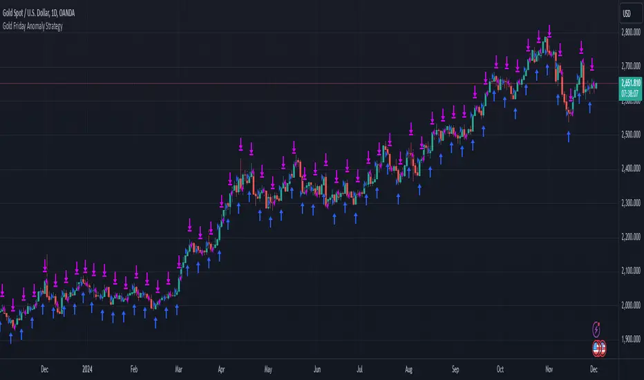
Gold Friday Anomaly StrategyThis script implements the " Gold Friday Anomaly Strategy ," a well-known historical trading strategy that leverages the gold market's behavior from Thursday evening to Friday close. It is a backtesting-focused strategy designed to assess the historical performance of this pattern. Traders use this anomaly as it captures a recurring market tendency observed over the years.
What It Does:
Entry Condition: The strategy enters a long position at the beginning of the Friday trading session (Thursday evening close) within the defined backtesting period.
Exit Condition: Friday evening close.
Backtesting Controls: Allows users to set custom backtesting periods to evaluate strategy performance over specific date ranges.
Key Features:
Custom Backtest Periods: Easily configurable inputs to set the start and end date of the backtesting range.
Fixed Slippage and Commission Settings: Ensures realistic simulation of trading conditions.
Process Orders on Close: Backtesting is optimized by processing orders at the bar's close.
Important Notes:
Backtesting Only: This script is intended purely for backtesting purposes. Past performance is not indicative of future results.
Live Trading Recommendations: For live trading, it is highly recommended to use limit orders instead of market orders, especially during evening sessions, as market order slippage can be significant.
Default Settings:
Entry size: 10% of equity per trade.
Slippage: 1 tick.
Commission: 0.05% per trade.
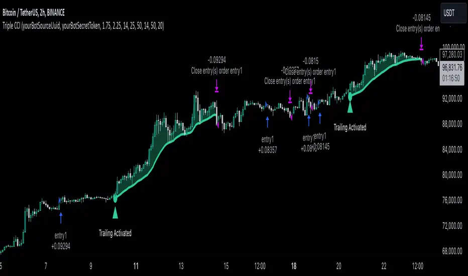
Triple CCI Strategy MFI Confirmed [Skyrexio]Overview
Triple CCI Strategy MFI Confirmed leverages 3 different periods Commodity Channel Index (CCI) indicator in conjunction Money Flow Index (MFI) and Exponential Moving Average (EMA) to obtain the high probability setups. Fast period CCI is used for having the high probability to enter in the direction of short term trend, middle and slow period CCI are used for confirmation, if market now likely in the mid and long-term uptrend. MFI is used to confirm trade with the money inflow/outflow with the high probability. EMA is used as an additional trend filter. Moreover, strategy uses exponential moving average (EMA) to trail the price when it reaches the specific level. More information in "Methodology" and "Justification of Methodology" paragraphs. The strategy opens only long trades.
Unique Features
Dynamic stop-loss system: Instead of fixed stop-loss level strategy utilizes average true range (ATR) multiplied by user given number subtracted from the position entry price as a dynamic stop loss level.
Configurable Trading Periods: Users can tailor the strategy to specific market windows, adapting to different market conditions.
Four layers trade filtering system: Strategy utilizes two different period CCI indicators, MFI and EMA indicators to confirm the signals produced by fast period CCI.
Trailing take profit level: After reaching the trailing profit activation level scrip activate the trailing of long trade using EMA. More information in methodology.
Methodology
The strategy opens long trade when the following price met the conditions:
Fast period CCI shall crossover the zero-line.
Slow and Middle period CCI shall be above zero-lines.
Price shall close above the EMA. Crossover is not obligatory
MFI shall be above 50
When long trade is executed, strategy set the stop-loss level at the price ATR multiplied by user-given value below the entry price. This level is recalculated on every next candle close, adjusting to the current market volatility.
At the same time strategy set up the trailing stop validation level. When the price crosses the level equals entry price plus ATR multiplied by user-given value script starts to trail the price with EMA. If price closes below EMA long trade is closed. When the trailing starts, script prints the label “Trailing Activated”.
Strategy settings
In the inputs window user can setup the following strategy settings:
ATR Stop Loss (by default = 1.75)
ATR Trailing Profit Activation Level (by default = 2.25)
CCI Fast Length (by default = 14, used for calculation short term period CCI)
CCI Middle Length (by default = 25, used for calculation short term period CCI)
CCI Slow Length (by default = 50, used for calculation long term period CCI)
MFI Length (by default = 14, used for calculation MFI
EMA Length (by default = 50, period of EMA, used for trend filtering EMA calculation)
Trailing EMA Length (by default = 20)
User can choose the optimal parameters during backtesting on certain price chart.
Justification of Methodology
Before understanding why this particular combination of indicator has been chosen let's briefly explain what is CCI, MFI and EMA.
The Commodity Channel Index (CCI) is a momentum-based technical indicator that measures the deviation of a security's price from its average price over a specific period. It helps traders identify overbought or oversold conditions and potential trend reversals.
The CCI formula is:
CCI = (Typical Price − SMA) / (0.015 × Mean Deviation)
Typical Price (TP): This is calculated as the average of the high, low, and closing prices for the period.
Simple Moving Average (SMA): This is the average of the Typical Prices over a specific number of periods.
Mean Deviation: This is the average of the absolute differences between the Typical Price and the SMA.
The result is a value that typically fluctuates between +100 and -100, though it is not bounded and can go higher or lower depending on the price movement.
The Money Flow Index (MFI) is a technical indicator that measures the strength of money flowing into and out of a security. It combines price and volume data to assess buying and selling pressure and is often used to identify overbought or oversold conditions. The formula for MFI involves several steps:
1. Calculate the Typical Price (TP):
TP = (high + low + close) / 3
2. Calculate the Raw Money Flow (RMF):
Raw Money Flow = TP × Volume
3. Determine Positive and Negative Money Flow:
If the current TP is greater than the previous TP, it's Positive Money Flow.
If the current TP is less than the previous TP, it's Negative Money Flow.
4. Calculate the Money Flow Ratio (MFR):
Money Flow Ratio = Sum of Positive Money Flow (over n periods) / Sum of Negative Money Flow (over n periods)
5. Calculate the Money Flow Index (MFI):
MFI = 100 − (100 / (1 + Money Flow Ratio))
MFI above 80 can be considered as overbought, below 20 - oversold.
The Exponential Moving Average (EMA) is a type of moving average that places greater weight and significance on the most recent data points. It is widely used in technical analysis to smooth price data and identify trends more quickly than the Simple Moving Average (SMA).
Formula:
1. Calculate the multiplier
Multiplier = 2 / (n + 1) , Where n is the number of periods.
2. EMA Calculation
EMA = (Current Price) × Multiplier + (Previous EMA) × (1 − Multiplier)
This strategy leverages Fast period CCI, which shall break the zero line to the upside to say that probability of short term trend change to the upside increased. This zero line crossover shall be confirmed by the Middle and Slow periods CCI Indicators. At the moment of breakout these two CCIs shall be above 0, indicating that there is a high probability that price is in middle and long term uptrend. This approach increases chances to have a long trade setup in the direction of mid-term and long-term trends when the short-term trend starts to reverse to the upside.
Additionally strategy uses MFI to have a greater probability that fast CCI breakout is confirmed by this indicator. We consider the values of MFI above 50 as a higher probability that trend change from downtrend to the uptrend is real. Script opens long trades only if MFI is above 50. As you already know from the MFI description, it incorporates volume in its calculation, therefore we have another one confirmation factor.
Finally, strategy uses EMA an additional trend filter. It allows to open long trades only if price close above EMA (by default 50 period). It increases the probability of taking long trades only in the direction of the trend.
ATR is used to adjust the strategy risk management to the current market volatility. If volatility is low, we don’t need the large stop loss to understand the there is a high probability that we made a mistake opening the trade. User can setup the settings ATR Stop Loss and ATR Trailing Profit Activation Level to realize his own risk to reward preferences, but the unique feature of a strategy is that after reaching trailing profit activation level strategy is trying to follow the trend until it is likely to be finished instead of using fixed risk management settings. It allows sometimes to be involved in the large movements. It’s also important to make a note, that script uses another one EMA (by default = 20 period) as a trailing profit level.
Backtest Results
Operating window: Date range of backtests is 2022.04.01 - 2024.11.25. It is chosen to let the strategy to close all opened positions.
Commission and Slippage: Includes a standard Binance commission of 0.1% and accounts for possible slippage over 5 ticks.
Initial capital: 10000 USDT
Percent of capital used in every trade: 50%
Maximum Single Position Loss: -4.13%
Maximum Single Profit: +19.66%
Net Profit: +5421.21 USDT (+54.21%)
Total Trades: 108 (44.44% win rate)
Profit Factor: 2.006
Maximum Accumulated Loss: 777.40 USDT (-7.77%)
Average Profit per Trade: 50.20 USDT (+0.85%)
Average Trade Duration: 44 hours
These results are obtained with realistic parameters representing trading conditions observed at major exchanges such as Binance and with realistic trading portfolio usage parameters.
How to Use
Add the script to favorites for easy access.
Apply to the desired timeframe and chart (optimal performance observed on 2h BTC/USDT).
Configure settings using the dropdown choice list in the built-in menu.
Set up alerts to automate strategy positions through web hook with the text: {{strategy.order.alert_message}}
Disclaimer:
Educational and informational tool reflecting Skyrex commitment to informed trading. Past performance does not guarantee future results. Test strategies in a simulated environment before live implementation
Max Pain StrategyThe Max Pain Strategy uses a combination of volume and price movement thresholds to identify potential "pain zones" in the market. A "pain zone" is considered when the volume exceeds a certain multiple of its average over a defined lookback period, and the price movement exceeds a predefined percentage relative to the price at the beginning of the lookback period.
Here’s how the strategy functions step-by-step:
Inputs:
length: Defines the lookback period used to calculate the moving average of volume and the price change over that period.
volMultiplier: Sets a threshold multiplier for the volume; if the volume exceeds the average volume multiplied by this factor, it triggers the condition for a potential "pain zone."
priceMultiplier: Sets a threshold for the minimum percentage price change that is required for a "pain zone" condition.
Calculations:
averageVolume: The simple moving average (SMA) of volume over the specified lookback period.
priceChange: The absolute difference in price between the current bar's close and the close from the lookback period (length).
Pain Zone Condition:
The condition for entering a position is triggered if both the volume is higher than the average volume by the volMultiplier and the price change exceeds the price at the length-period ago by the priceMultiplier. This is an indication of significant market activity that could result in a price move.
Position Entry:
A long position is entered when the "pain zone" condition is met.
Exit Strategy:
The position is closed after the specified holdPeriods, which defines how many periods the position will be held after being entered.
Visualization:
A small triangle is plotted on the chart where the "pain zone" condition is met.
The background color changes to a semi-transparent red when the "pain zone" is active.
Scientific Explanation of the Components
Volume Analysis and Price Movement: These are two critical factors in trading strategies. Volume often serves as an indicator of market strength (or weakness), and price movement is a direct reflection of market sentiment. Higher volume with significant price movement may suggest that the market is entering a phase of increased volatility or trend formation, which the strategy aims to exploit.
Volume analysis: The study of volume as an indicator of market participation, with increased volume often signaling stronger trends (Murphy, J. J., Technical Analysis of the Financial Markets).
Price movement thresholds: A large price change over a short period may be interpreted as a breakout or a potential reversal point, aligning with volatility and liquidity analysis (Schwager, J. D., Market Wizards).
Repainting Check: This strategy does not involve any repainting because it is based on current and past data, and there is no reference to future values in the decision-making process. However, any strategy that uses lagging indicators or conditions based on historical bars, like close , is inherently a lagging strategy and might not predict real-time price action accurately until after the fact.
Risk Management: The position hold duration is predefined, which adds an element of time-based risk control. This duration ensures that the strategy does not hold a position indefinitely, which could expose it to unnecessary risk.
Potential Issues and Considerations
Repainting:
The strategy does not utilize future data or conditions that depend on future bars, so it does not inherently suffer from repainting issues.
However, since the strategy relies on volume and price change over a set lookback period, the decision to enter or exit a trade is only made after the data for the current bar is complete, meaning the trade decisions are somewhat delayed, which could be seen as a lagging feature rather than a repainting one.
Lagging Nature:
As with many technical analysis-based strategies, this one is based on past data (moving averages, price changes), meaning it reacts to market movements after they have already occurred, rather than predicting future price actions.
Overfitting Risk:
With parameters like the lookback period and multipliers being user-adjustable, there is a risk of overfitting to historical data. Adjusting parameters too much based on past performance can lead to poor out-of-sample results (Gauthier, P., Practical Quantitative Finance).
Conclusion
The Max Pain Strategy is a simple approach to identifying potential market entries based on volume spikes and significant price changes. It avoids repainting by relying solely on historical and current bar data, but it is inherently a lagging strategy that reacts to price and volume patterns after they have occurred. Therefore, the strategy can be effective in trending markets but may struggle in highly volatile, sideways markets.

The Most Powerful TQQQ EMA Crossover Trend Trading StrategyTQQQ EMA Crossover Strategy Indicator
Meta Title: TQQQ EMA Crossover Strategy - Enhance Your Trading with Effective Signals
Meta Description: Discover the TQQQ EMA Crossover Strategy, designed to optimize trading decisions with fast and slow EMA crossovers. Learn how to effectively use this powerful indicator for better trading results.
Key Features
The TQQQ EMA Crossover Strategy is a powerful trading tool that utilizes Exponential Moving Averages (EMAs) to identify potential entry and exit points in the market. Key features of this indicator include:
**Fast and Slow EMAs:** The strategy incorporates two EMAs, allowing traders to capture short-term trends while filtering out market noise.
**Entry and Exit Signals:** Automated signals for entering and exiting trades based on EMA crossovers, enhancing decision-making efficiency.
**Customizable Parameters:** Users can adjust the lengths of the EMAs, as well as take profit and stop loss multipliers, tailoring the strategy to their trading style.
**Visual Indicators:** Clear visual plots of the EMAs and exit points on the chart for easy interpretation.
How It Works
The TQQQ EMA Crossover Strategy operates by calculating two EMAs: a fast EMA (default length of 20) and a slow EMA (default length of 50). The core concept is based on the crossover of these two moving averages:
- When the fast EMA crosses above the slow EMA, it generates a *buy signal*, indicating a potential upward trend.
- Conversely, when the fast EMA crosses below the slow EMA, it produces a *sell signal*, suggesting a potential downward trend.
This method allows traders to capitalize on momentum shifts in the market, providing timely signals for trade execution.
Trading Ideas and Insights
Traders can leverage the TQQQ EMA Crossover Strategy in various market conditions. Here are some insights:
**Scalping Opportunities:** The strategy is particularly effective for scalping in volatile markets, allowing traders to make quick profits on small price movements.
**Swing Trading:** Longer-term traders can use this strategy to identify significant trend reversals and capitalize on larger price swings.
**Risk Management:** By incorporating customizable stop loss and take profit levels, traders can manage their risk effectively while maximizing potential returns.
How Multiple Indicators Work Together
While this strategy primarily relies on EMAs, it can be enhanced by integrating additional indicators such as:
- **Relative Strength Index (RSI):** To confirm overbought or oversold conditions before entering trades.
- **Volume Indicators:** To validate breakout signals, ensuring that price movements are supported by sufficient trading volume.
Combining these indicators provides a more comprehensive view of market dynamics, increasing the reliability of trade signals generated by the EMA crossover.
Unique Aspects
What sets this indicator apart is its simplicity combined with effectiveness. The reliance on EMAs allows for smoother signals compared to traditional moving averages, reducing false signals often associated with choppy price action. Additionally, the ability to customize parameters ensures that traders can adapt the strategy to fit their unique trading styles and risk tolerance.
How to Use
To effectively utilize the TQQQ EMA Crossover Strategy:
1. **Add the Indicator:** Load the script onto your TradingView chart.
2. **Set Parameters:** Adjust the fast and slow EMA lengths according to your trading preferences.
3. **Monitor Signals:** Watch for crossover points; enter trades based on buy/sell signals generated by the indicator.
4. **Implement Risk Management:** Set your stop loss and take profit levels using the provided multipliers.
Regularly review your trading performance and adjust parameters as necessary to optimize results.
Customization
The TQQQ EMA Crossover Strategy allows for extensive customization:
- **EMA Lengths:** Change the default lengths of both fast and slow EMAs to suit different time frames or market conditions.
- **Take Profit/Stop Loss Multipliers:** Adjust these values to align with your risk management strategy. For instance, increasing the take profit multiplier may yield larger gains but could also increase exposure to market fluctuations.
This flexibility makes it suitable for various trading styles, from aggressive scalpers to conservative swing traders.
Conclusion
The TQQQ EMA Crossover Strategy is an effective tool for traders seeking an edge in their trading endeavors. By utilizing fast and slow EMAs, this indicator provides clear entry and exit signals while allowing for customization to fit individual trading strategies. Whether you are a scalper looking for quick profits or a swing trader aiming for larger moves, this indicator offers valuable insights into market trends.
Incorporate it into your TradingView toolkit today and elevate your trading performance!

S&P 100 Option Expiration Week StrategyThe Option Expiration Week Strategy aims to capitalize on increased volatility and trading volume that often occur during the week leading up to the expiration of options on stocks in the S&P 100 index. This period, known as the option expiration week, culminates on the third Friday of each month when stock options typically expire in the U.S. During this week, investors in this strategy take a long position in S&P 100 stocks or an equivalent ETF from the Monday preceding the third Friday, holding until Friday. The strategy capitalizes on potential upward price pressures caused by increased option-related trading activity, rebalancing, and hedging practices.
The phenomenon leveraged by this strategy is well-documented in finance literature. Studies demonstrate that options expiration dates have a significant impact on stock returns, trading volume, and volatility. This effect is driven by various market dynamics, including portfolio rebalancing, delta hedging by option market makers, and the unwinding of positions by institutional investors (Stoll & Whaley, 1987; Ni, Pearson, & Poteshman, 2005). These market activities intensify near option expiration, causing price adjustments that may create short-term profitable opportunities for those aware of these patterns (Roll, Schwartz, & Subrahmanyam, 2009).
The paper by Johnson and So (2013), Returns and Option Activity over the Option-Expiration Week for S&P 100 Stocks, provides empirical evidence supporting this strategy. The study analyzes the impact of option expiration on S&P 100 stocks, showing that these stocks tend to exhibit abnormal returns and increased volume during the expiration week. The authors attribute these patterns to intensified option trading activity, where demand for hedging and arbitrage around options expiration causes temporary price adjustments.
Scientific Explanation
Research has found that option expiration weeks are marked by predictable increases in stock returns and volatility, largely due to the role of options market makers and institutional investors. Option market makers often use delta hedging to manage exposure, which requires frequent buying or selling of the underlying stock to maintain a hedged position. As expiration approaches, their activity can amplify price fluctuations. Additionally, institutional investors often roll over or unwind positions during expiration weeks, creating further demand for underlying stocks (Stoll & Whaley, 1987). This increased demand around expiration week typically leads to temporary stock price increases, offering profitable opportunities for short-term strategies.
Key Research and Bibliography
Johnson, T. C., & So, E. C. (2013). Returns and Option Activity over the Option-Expiration Week for S&P 100 Stocks. Journal of Banking and Finance, 37(11), 4226-4240.
This study specifically examines the S&P 100 stocks and demonstrates that option expiration weeks are associated with abnormal returns and trading volume due to increased activity in the options market.
Stoll, H. R., & Whaley, R. E. (1987). Program Trading and Expiration-Day Effects. Financial Analysts Journal, 43(2), 16-28.
Stoll and Whaley analyze how program trading and portfolio insurance strategies around expiration days impact stock prices, leading to temporary volatility and increased trading volume.
Ni, S. X., Pearson, N. D., & Poteshman, A. M. (2005). Stock Price Clustering on Option Expiration Dates. Journal of Financial Economics, 78(1), 49-87.
This paper investigates how option expiration dates affect stock price clustering and volume, driven by delta hedging and other option-related trading activities.
Roll, R., Schwartz, E., & Subrahmanyam, A. (2009). Options Trading Activity and Firm Valuation. Journal of Financial Markets, 12(3), 519-534.
The authors explore how options trading activity influences firm valuation, finding that higher options volume around expiration dates can lead to temporary price movements in underlying stocks.
Cao, C., & Wei, J. (2010). Option Market Liquidity and Stock Return Volatility. Journal of Financial and Quantitative Analysis, 45(2), 481-507.
This study examines the relationship between options market liquidity and stock return volatility, finding that increased liquidity needs during expiration weeks can heighten volatility, impacting stock returns.
Summary
The Option Expiration Week Strategy utilizes well-researched financial market phenomena related to option expiration. By positioning long in S&P 100 stocks or ETFs during this period, traders can potentially capture abnormal returns driven by option market dynamics. The literature suggests that options-related activities—such as delta hedging, position rollovers, and portfolio adjustments—intensify demand for underlying assets, creating short-term profit opportunities around these key dates.

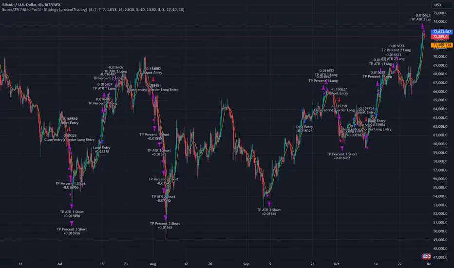
SuperATR 7-Step Profit - Strategy [presentTrading] Long time no see!
█ Introduction and How It Is Different
The SuperATR 7-Step Profit Strategy is a multi-layered trading approach that integrates adaptive Average True Range (ATR) calculations with momentum-based trend detection. What sets this strategy apart is its sophisticated 7-step take-profit mechanism, which combines four ATR-based exit levels and three fixed percentage levels. This hybrid approach allows traders to dynamically adjust to market volatility while systematically capturing profits in both long and short market positions.
Traditional trading strategies often rely on static indicators or single-layered exit strategies, which may not adapt well to changing market conditions. The SuperATR 7-Step Profit Strategy addresses this limitation by:
- Using Adaptive ATR: Enhances the standard ATR by making it responsive to current market momentum.
- Incorporating Momentum-Based Trend Detection: Identifies stronger trends with higher probability of continuation.
- Employing a Multi-Step Take-Profit System: Allows for gradual profit-taking at predetermined levels, optimizing returns while minimizing risk.
BTCUSD 6hr Performance
█ Strategy, How It Works: Detailed Explanation
The strategy revolves around detecting strong market trends and capitalizing on them using an adaptive ATR and momentum indicators. Below is a detailed breakdown of each component of the strategy.
🔶 1. True Range Calculation with Enhanced Volatility Detection
The True Range (TR) measures market volatility by considering the most significant price movements. The enhanced TR is calculated as:
TR = Max
Where:
High and Low are the current bar's high and low prices.
Previous Close is the closing price of the previous bar.
Abs denotes the absolute value.
Max selects the maximum value among the three calculations.
🔶 2. Momentum Factor Calculation
To make the ATR adaptive, the strategy incorporates a Momentum Factor (MF), which adjusts the ATR based on recent price movements.
Momentum = Close - Close
Stdev_Close = Standard Deviation of Close over n periods
Normalized_Momentum = Momentum / Stdev_Close (if Stdev_Close ≠ 0)
Momentum_Factor = Abs(Normalized_Momentum)
Where:
Close is the current closing price.
n is the momentum_period, a user-defined input (default is 7).
Standard Deviation measures the dispersion of closing prices over n periods.
Abs ensures the momentum factor is always positive.
🔶 3. Adaptive ATR Calculation
The Adaptive ATR (AATR) adjusts the traditional ATR based on the Momentum Factor, making it more responsive during volatile periods and smoother during consolidation.
Short_ATR = SMA(True Range, short_period)
Long_ATR = SMA(True Range, long_period)
Adaptive_ATR = /
Where:
SMA is the Simple Moving Average.
short_period and long_period are user-defined inputs (defaults are 3 and 7, respectively).
🔶 4. Trend Strength Calculation
The strategy quantifies the strength of the trend to filter out weak signals.
Price_Change = Close - Close
ATR_Multiple = Price_Change / Adaptive_ATR (if Adaptive_ATR ≠ 0)
Trend_Strength = SMA(ATR_Multiple, n)
🔶 5. Trend Signal Determination
If (Short_MA > Long_MA) AND (Trend_Strength > Trend_Strength_Threshold):
Trend_Signal = 1 (Strong Uptrend)
Elif (Short_MA < Long_MA) AND (Trend_Strength < -Trend_Strength_Threshold):
Trend_Signal = -1 (Strong Downtrend)
Else:
Trend_Signal = 0 (No Clear Trend)
🔶 6. Trend Confirmation with Price Action
Adaptive_ATR_SMA = SMA(Adaptive_ATR, atr_sma_period)
If (Trend_Signal == 1) AND (Close > Short_MA) AND (Adaptive_ATR > Adaptive_ATR_SMA):
Trend_Confirmed = True
Elif (Trend_Signal == -1) AND (Close < Short_MA) AND (Adaptive_ATR > Adaptive_ATR_SMA):
Trend_Confirmed = True
Else:
Trend_Confirmed = False
Local Performance
🔶 7. Multi-Step Take-Profit Mechanism
The strategy employs a 7-step take-profit system
█ Trade Direction
The SuperATR 7-Step Profit Strategy is designed to work in both long and short market conditions. By identifying strong uptrends and downtrends, it allows traders to capitalize on price movements in either direction.
Long Trades: Initiated when the market shows strong upward momentum and the trend is confirmed.
Short Trades: Initiated when the market exhibits strong downward momentum and the trend is confirmed.
█ Usage
To implement the SuperATR 7-Step Profit Strategy:
1. Configure the Strategy Parameters:
- Adjust the short_period, long_period, and momentum_period to match the desired sensitivity.
- Set the trend_strength_threshold to control how strong a trend must be before acting.
2. Set Up the Multi-Step Take-Profit Levels:
- Define ATR multipliers and fixed percentage levels according to risk tolerance and profit goals.
- Specify the percentage of the position to close at each level.
3. Apply the Strategy to a Chart:
- Use the strategy on instruments and timeframes where it has been tested and optimized.
- Monitor the positions and adjust parameters as needed based on performance.
4. Backtest and Optimize:
- Utilize TradingView's backtesting features to evaluate historical performance.
- Adjust the default settings to optimize for different market conditions.
█ Default Settings
Understanding default settings is crucial for optimal performance.
Short Period (3): Affects the responsiveness of the short-term MA.
Effect: Lower values increase sensitivity but may produce more false signals.
Long Period (7): Determines the trend baseline.
Effect: Higher values reduce noise but may delay signals.
Momentum Period (7): Influences adaptive ATR and trend strength.
Effect: Shorter periods react quicker to price changes.
Trend Strength Threshold (0.5): Filters out weaker trends.
Effect: Higher thresholds yield fewer but stronger signals.
ATR Multipliers: Set distances for ATR-based exits.
Effect: Larger multipliers aim for bigger moves but may reduce hit rate.
Fixed TP Levels (%): Control profit-taking on smaller moves.
Effect: Adjusting these levels affects how quickly profits are realized.
Exit Percentages: Determine how much of the position is closed at each TP level.
Effect: Higher percentages reduce exposure faster, affecting risk and reward.
Adjusting these variables allows you to tailor the strategy to different market conditions and personal risk preferences.
By integrating adaptive indicators and a multi-tiered exit strategy, the SuperATR 7-Step Profit Strategy offers a versatile tool for traders seeking to navigate varying market conditions effectively. Understanding and adjusting the key parameters enables traders to harness the full potential of this strategy.
Strategy: Candlestick Wick Analysis with Volume Conditions
This strategy focuses on analyzing the wicks (or shadows) of candlesticks to identify potential trading opportunities based on candlestick structure and volume. Based on these criteria, it places stop orders at the extremities of the wicks when certain conditions are met, thus increasing the chances of capturing significant price movements.
Trading Criteria
Volume Conditions:
The strategy checks if the volume of the current candle is higher than that of the previous three candles. This ensures that the observed price movement is supported by significant volume, increasing the probability that the price will continue in the same direction.
Wick Analysis:
Upper Wick:
If the upper wick of a candle represents more than 90% of its body size and is longer than the lower wick, this indicates that the price tested a resistance level before pulling back.
Order Placement: In this case, a Buy Stop order is placed at the upper extremity of the wick. This means that if the price rises back to this level, the order will be triggered, and the trader will take a buy position.
SL Management: A stop-loss is then placed below the lowest point of the same candle. This protects the trader by limiting losses if the price falls back after the order is triggered.
Lower Wick:
If the lower wick of a candle is longer than the upper wick and represents more than 90% of its body size, this indicates that the price tested a support level before rising.
Order Placement: In this case, a Sell Stop order is placed at the lower extremity of the wick. Thus, if the price drops back to this level, the order will be triggered, and the trader will take a sell position.
SL Management: A stop-loss is then placed above the highest point of the same candle. This ensures risk management by limiting losses if the price rebounds upward after the order is triggered.
Strategy Advantages
Responsiveness to Price Movements: The strategy is designed to detect significant price movements based on the market's reaction around support and resistance levels. By placing stop orders directly at the wick extremities, it allows capturing strong movements in the direction indicated by the candles.
Securing Positions: Using stop-losses positioned just above or below key levels (wicks) provides better risk management. If the market doesn't move as expected, the position is automatically closed with a limited loss.
Clear Visual Indicators: Symbols are displayed on the chart at the points where orders have been placed, making it easier to understand trading decisions. This helps to quickly identify the support or resistance levels tested by the price, as well as potential entry points.
Conclusion
The strategy is based on the idea that large wicks signal areas where buyers or sellers have tested significant price levels before temporarily retreating. By placing stop orders at the extremities of these wicks, the strategy allows capturing price movements when they confirm, while limiting risks through strategically placed stop-losses. It thus offers a balanced approach between capturing potential profit and managing risk.
This description emphasizes the idea of capturing significant market movements with stop orders while providing a clear explanation of the logic and risk management. It’s tailored for publication on TradingView and highlights the robustness of the strategy.
3-Bar (Outside Bar) Scanner with Table Display# 3-Bar (Outside Bar) Scanner with Table Display
## Overview
The **3-Bar (Outside Bar) Scanner with Table Display** is a custom TradingView indicator designed for traders who utilize **The Strat** methodology. This indicator scans for **3-bar (Outside Bar)** patterns across multiple symbols and displays the results in a convenient table format directly on your chart.
## Purpose
- **Efficient Multi-Symbol Scanning**: Monitor up to four symbols simultaneously for 3-bar patterns without the need to switch between charts.
- **Real-Time Updates**: The table dynamically updates with new price data, providing immediate insights into potential trading opportunities.
- **Visual Clarity**: Displays whether a 3-bar is bullish ("3 Up") or bearish ("3 Down"), helping you quickly interpret market sentiment.
## How It Works
- **Data Retrieval**: The indicator uses `request.security()` to fetch high, low, open, and close prices for the specified symbols and timeframe.
- **3-Bar Detection**:
- **Outside Bar Criteria**: Checks if the current candle's high is higher than the previous candle's high and the current low is lower than the previous low.
- **Direction Determination**:
- **"3 Up"**: If the candle closes higher than it opens (bullish candle).
- **"3 Down"**: If the candle closes lower than it opens (bearish candle).
- **Table Display**:
- The table shows the **Symbol**, **Timeframe**, and **State** ("3 Up", "3 Down", or blank if no pattern detected).
- Customizable colors and positioning to fit your chart's aesthetics.
## Best Use Cases
- **Rapid Market Analysis**: Ideal for traders needing a quick overview of multiple assets for potential 3-bar setups.
- **Strategic Decision-Making**: Helps identify key reversal or continuation patterns in alignment with **The Strat** principles.
- **Scalable Monitoring**: By utilizing TradingView's multi-chart layouts, you can expand monitoring beyond four symbols.
## Instructions for Use
### Adding the Indicator to Your Chart
1. **Copy the Code**: Use the provided Pine Script code for the indicator.
2. **Create a New Indicator**:
- In TradingView, click on **Pine Editor** at the bottom of the platform.
- Paste the code into the editor.
3. **Save and Add to Chart**:
- Click **Save** and give your indicator a name.
- Click **Add to Chart** to apply it.
### Customizing the Inputs
- **Symbols**:
- **Symbol 1**: Leave blank to use the current chart's symbol or enter a specific symbol (e.g., `AAPL`).
- **Symbol 2 to Symbol 4**: Enter additional symbols or leave them blank.
- **Timeframe**: Select your desired timeframe (e.g., `D` for Daily, `60` for 60-minute).
- **Table Colors**:
- Customize header and data colors for better visibility against your chart background.
### Interpreting the Table
- **Symbol**: Displays the symbol without the exchange prefix for clarity.
- **Timeframe**: Shows the timeframe applied to the analysis.
- **State**:
- **"3 Up"**: A bullish outside bar where the candle closed higher than it opened.
- **"3 Down"**: A bearish outside bar where the candle closed lower than it opened.
- **Blank**: No 3-bar pattern detected on the latest candle.
### Monitoring More Than Four Symbols
- **Multi-Chart Layout**:
- Use TradingView's multi-chart feature to display multiple charts within a single workspace.
- Apply the indicator to each chart. For example:
- **Four-Chart Grid**: Monitor up to 16 symbols by setting up four charts, each with the indicator tracking four symbols.
- **Steps**:
1. Arrange your workspace into a multi-chart layout.
2. Add the indicator to each chart.
3. Input different symbols into the indicator on each chart.
## Example Usage
Suppose you want to monitor the following symbols on a Daily timeframe:
- **Symbol 1**: *(Leave blank to use the current chart's symbol, e.g., `SPY`)*
- **Symbol 2**: `AAPL`
- **Symbol 3**: `TSLA`
- **Symbol 4**: `AMZN`
After adding the indicator and entering these symbols:
- **SPY**: The table shows "3 Up" in the State column, indicating a bullish outside bar.
- **AAPL**: No 3-bar pattern detected; the State column is blank.
- **TSLA**: The table shows "3 Down," indicating a bearish outside bar.
- **AMZN**: The table shows "3 Up," indicating another bullish outside bar.
This setup allows you to quickly assess which symbols are exhibiting significant patterns that may warrant further analysis or action.
## Notes
- **Customization**: Feel free to adjust the table's position and colors to suit your preferences.
- **Limitations**:
- Be aware of TradingView's limitations on `request.security()` calls, which may vary based on your subscription plan.
- The indicator is designed to monitor up to four symbols per instance due to these limitations.
- **Scalability**:
- By using multi-chart layouts, you can effectively monitor more symbols without overloading a single chart.
- This approach allows you to scale up your monitoring capabilities to fit your trading strategy.
## Conclusion
The **3-Bar (Outside Bar) Scanner with Table Display** is a valuable tool for traders who utilize **The Strat** methodology. It streamlines the process of identifying key 3-bar patterns across multiple symbols and timeframes, enhancing your ability to make informed trading decisions quickly.
By integrating this indicator into your trading routine, you can:
- Stay alert to significant market movements.
- Reduce the time spent manually scanning charts.
- Increase efficiency in executing your trading strategy.
---
Feel free to share this indicator with the Strat community. Feedback and suggestions are welcome to further enhance its functionality. Happy trading!

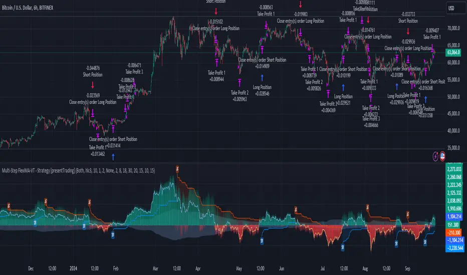
Multi-Step FlexiMA - Strategy [presentTrading]It's time to come back! hope I can not to be busy for a while.
█ Introduction and How It Is Different
The FlexiMA Variance Tracker is a unique trading strategy that calculates a series of deviations between the price (or another indicator source) and a variable-length moving average (MA). Unlike traditional strategies that use fixed-length moving averages, the length of the MA in this system varies within a defined range. The length changes dynamically based on a starting factor and an increment factor, creating a more adaptive approach to market conditions.
This strategy integrates Multi-Step Take Profit (TP) levels, allowing for partial exits at predefined price increments. It enables traders to secure profits at different stages of a trend, making it ideal for volatile markets where taking full profits at once might lead to missed opportunities if the trend continues.
BTCUSD 6hr Performance
█ Strategy, How It Works: Detailed Explanation
🔶 FlexiMA Concept
The FlexiMA (Flexible Moving Average) is at the heart of this strategy. Unlike traditional MA-based strategies where the MA length is fixed (e.g., a 50-period SMA), the FlexiMA varies its length with each iteration. This is done using a **starting factor** and an **increment factor**.
The formula for the moving average length at each iteration \(i\) is:
`MA_length_i = indicator_length * (starting_factor + i * increment_factor)`
Where:
- `indicator_length` is the user-defined base length.
- `starting_factor` is the initial multiplier of the base length.
- `increment_factor` increases the multiplier in each iteration.
Each iteration applies a **simple moving average** (SMA) to the chosen **indicator source** (e.g., HLC3) with a different length based on the above formula. The deviation between the current price and the moving average is then calculated as follows:
`deviation_i = price_current - MA_i`
These deviations are normalized using one of the following methods:
- **Max-Min normalization**:
`normalized_i = (deviation_i - min(deviations)) / range(deviations)`
- **Absolute Sum normalization**:
`normalized_i = deviation_i / sum(|deviation_i|)`
The **median** and **standard deviation (stdev)** of the normalized deviations are then calculated as follows:
`median = median(normalized deviations)`
For the standard deviation:
`stdev = sqrt((1/(N-1)) * sum((normalized_i - mean)^2))`
These values are plotted to provide a clear indication of how the price is deviating from its variable-length moving averages.
For more detail:
🔶 Multi-Step Take Profit
This strategy uses a multi-step take profit system, allowing for exits at different stages of a trade based on the percentage of price movement. Three take-profit levels are defined:
- Take Profit Level 1 (TP1): A small, quick profit level (e.g., 2%).
- Take Profit Level 2 (TP2): A medium-level profit target (e.g., 8%).
- Take Profit Level 3 (TP3): A larger, more ambitious target (e.g., 18%).
At each level, a corresponding percentage of the trade is exited:
- TP Percent 1: E.g., 30% of the position.
- TP Percent 2: E.g., 20% of the position.
- TP Percent 3: E.g., 15% of the position.
This approach ensures that profits are locked in progressively, reducing the risk of market reversals wiping out potential gains.
Local
🔶 Trade Entry and Exit Conditions
The entry and exit signals are determined by the interaction between the **SuperTrend Polyfactor Oscillator** and the **median** value of the normalized deviations:
- Long entry: The SuperTrend turns bearish, and the median value of the deviations is positive.
- Short entry: The SuperTrend turns bullish, and the median value is negative.
Similarly, trades are exited when the SuperTrend flips direction.
* The SuperTrend Toolkit is made by @EliCobra
█ Trade Direction
The strategy allows users to specify the desired trade direction:
- Long: Only long positions will be taken.
- Short: Only short positions will be taken.
- Both: Both long and short positions are allowed based on the conditions.
This flexibility allows the strategy to adapt to different market conditions and trading styles, whether you're looking to buy low and sell high, or sell high and buy low.
█ Usage
This strategy can be applied across various asset classes, including stocks, cryptocurrencies, and forex. The primary use case is to take advantage of market volatility by using a flexible moving average and multiple take-profit levels to capture profits incrementally as the market moves in your favor.
How to Use:
1. Configure the Inputs: Start by adjusting the **Indicator Length**, **Starting Factor**, and **Increment Factor** to suit your chosen asset. The defaults work well for most markets, but fine-tuning them can improve performance.
2. Set the Take Profit Levels: Adjust the three **TP levels** and their corresponding **percentages** based on your risk tolerance and the expected volatility of the market.
3. Monitor the Strategy: The SuperTrend and the FlexiMA variance tracker will provide entry and exit signals, automatically managing the positions and taking profits at the pre-set levels.
█ Default Settings
The default settings for the strategy are configured to provide a balanced approach that works across different market conditions:
Indicator Length (10):
This controls the base length for the moving average. A lower length makes the moving average more responsive to price changes, while a higher length smooths out fluctuations, making the strategy less sensitive to short-term price movements.
Starting Factor (1.0):
This determines the initial multiplier applied to the moving average length. A higher starting factor will increase the average length, making it slower to react to price changes.
Increment Factor (1.0):
This increases the moving average length in each iteration. A larger increment factor creates a wider range of moving average lengths, allowing the strategy to track both short-term and long-term trends simultaneously.
Normalization Method ('None'):
Three methods of normalization can be applied to the deviations:
- None: No normalization applied, using raw deviations.
- Max-Min: Normalizes based on the range between the maximum and minimum deviations.
- Absolute Sum: Normalizes based on the total sum of absolute deviations.
Take Profit Levels:
- TP1 (2%): A quick exit to capture small price movements.
- TP2 (8%): A medium-term profit target for stronger trends.
- TP3 (18%): A long-term target for strong price moves.
Take Profit Percentages:
- TP Percent 1 (30%): Exits 30% of the position at TP1.
- TP Percent 2 (20%): Exits 20% of the position at TP2.
- TP Percent 3 (15%): Exits 15% of the position at TP3.
Effect of Variables on Performance:
- Short Indicator Lengths: More responsive to price changes but prone to false signals.
- Higher Starting Factor: Slows down the response, useful for longer-term trend following.
- Higher Increment Factor: Widens the variability in moving average lengths, making the strategy adapt to both short-term and long-term price trends.
- Aggressive Take Profit Levels: Allows for quick profit-taking in volatile markets but may exit positions prematurely in strong trends.
The default configuration offers a moderate balance between short-term responsiveness and long-term trend capturing, suitable for most traders. However, users can adjust these variables to optimize performance based on market conditions and personal preferences.
Larry Conners SMTP StrategyThe Spent Market Trading Pattern is a strategy developed by Larry Connors, typically used for short-term mean reversion trading. This strategy takes advantage of the exhaustion in market momentum by entering trades when the market is perceived as "spent" after extended trends or extreme moves, expecting a short-term reversal. Connors uses indicators like RSI (Relative Strength Index) and price action patterns to identify these opportunities.
Key Elements of the Strategy:
Overbought/Oversold Conditions: The strategy looks for extreme overbought or oversold conditions, often indicated by low RSI values (below 30 for oversold and above 70 for overbought).
Mean Reversion: Connors believed that markets, especially in short-term scenarios, tend to revert to the mean after periods of strong momentum. The "spent" market is assumed to have expended its energy, making a reversal likely.
Entry Signals:
In an uptrend, a stock or market index making a significant number of consecutive up days (e.g., 5-7 consecutive days with higher closes) indicates overbought conditions.
In a downtrend, a similar number of consecutive down days indicates oversold conditions.
Reversal Anticipation: Once an extreme in price movement is identified (such as consecutive gains or losses), the strategy places trades anticipating a reversion to the mean, which is usually the 5-day or 10-day moving average.
Exit Points: Trades are exited when prices move back toward their mean or when the extreme conditions dissipate, usually based on RSI or moving average thresholds.
Why the Strategy Works:
Human Psychology: The strategy capitalizes on the fact that markets, in the short term, often behave irrationally due to the emotions of traders—fear and greed lead to overextended moves.
Mean Reversion Tendency: Financial markets often exhibit mean-reverting behavior, where prices temporarily deviate from their historical norms but eventually return. Short-term exhaustion after a strong rally or sell-off offers opportunities for quick profits.
Overextended Moves: Markets that rise or fall too quickly tend to become overextended, as buyers or sellers get exhausted, making reversals more probable. Connors’ approach identifies these moments when the market is "spent" and ripe for a reversal.
Risks of the Spent Market Trading Pattern Strategy:
Trend Continuation: One of the key risks is that the market may not revert as expected and instead continues in the same direction. In trending markets, mean-reversion strategies can suffer because strong trends can last longer than anticipated.
False Signals: The strategy relies heavily on technical indicators like RSI, which can produce false signals in volatile or choppy markets. There can be times when a market appears "spent" but continues in its current direction.
Market Timing: Mean reversion strategies often require precise market timing. If the entry or exit points are mistimed, it can lead to losses, especially in short-term trades where small price movements can significantly impact profitability.
High Transaction Costs: This strategy requires frequent trades, which can lead to higher transaction costs, especially in markets with wide bid-ask spreads or high commissions.
Conclusion:
Larry Connors’ Spent Market Trading Pattern strategy is built on the principle of mean reversion, leveraging the concept that markets tend to revert to a mean after extreme moves. While effective in certain conditions, such as range-bound markets, it carries risks—especially during strong trends—where price momentum may not reverse as quickly as expected.
For a more in-depth explanation, Larry Connors’ books such as "Short-Term Trading Strategies That Work" provide a comprehensive guide to this and other strategies .
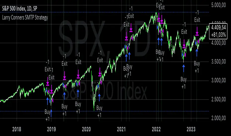
Connors VIX Reversal III invented by Dave LandryThis strategy is based on trading signals derived from the behavior of the Volatility Index (VIX) relative to its 10-day moving average. The rules are split into buying and selling conditions:
Buy Conditions:
The VIX low must be above its 10-day moving average.
The VIX must close at least 10% above its 10-day moving average.
If both conditions are met, a buy signal is generated at the market's close.
Sell Conditions:
The VIX high must be below its 10-day moving average.
The VIX must close at least 10% below its 10-day moving average.
If both conditions are met, a sell signal is generated at the market's close.
Exit Conditions:
For long positions, the strategy exits when the VIX trades intraday below its previous day’s 10-day moving average.
For short positions, the strategy exits when the VIX trades intraday above its previous day’s 10-day moving average.
This strategy is primarily a mean-reversion strategy, where the market is expected to revert to a more normal state after the VIX exhibits extreme behavior (i.e., large deviations from its moving average).
About Dave Landry
Dave Landry is a well-known figure in the world of trading, particularly in technical analysis. He is an author, trader, and educator, best known for his work on swing trading strategies. Landry focuses on trend-following and momentum-based techniques, teaching traders how to capitalize on shorter-term price swings in the market. He has written books like "Dave Landry on Swing Trading" and "The Layman's Guide to Trading Stocks," which emphasize practical, actionable trading strategies.
About Connors Research
Connors Research is a financial research firm known for its quantitative research in financial markets. Founded by Larry Connors, the firm specializes in developing high-probability trading systems based on historical market behavior. Connors’ work is widely respected for its data-driven approach, including systems like the RSI(2) strategy, which focuses on short-term mean reversion. The firm also provides trading education and tools for institutional and retail traders alike, emphasizing strategies that can be backtested and quantified.
Risks of the Strategy
While this strategy may appear to offer promising opportunities to exploit extreme VIX movements, it carries several risks:
Market Volatility: The VIX itself is a measure of market volatility, meaning the strategy can be exposed to sudden and unpredictable market swings. This can result in whipsaws, where positions are opened and closed in rapid succession due to sharp reversals in the VIX.
Overfitting: Strategies based on specific conditions like the VIX closing 10% above or below its moving average can be subject to overfitting, meaning they work well in historical tests but may underperform in live markets. This is a common issue in quantitative trading systems that are not adaptable to changing market conditions .
Mean-Reversion Assumption: The core assumption behind this strategy is that markets will revert to their mean after extreme movements. However, during periods of sustained trends (e.g., market crashes or rallies), this assumption may break down, leading to prolonged drawdowns.
Liquidity and Slippage: Depending on the asset being traded (e.g., S&P 500 futures, ETFs), liquidity issues or slippage could occur when executing trades at market close, particularly in volatile conditions. This could increase costs or worsen trade execution.
Scientific Explanation of the Strategy
The VIX is often referred to as the "fear gauge" because it measures the market's expectations of volatility based on options prices. Research has shown that the VIX tends to spike during periods of market stress and revert to lower levels when conditions stabilize . Mean reversion strategies like this one assume that extreme VIX levels are unsustainable in the long run, which aligns with findings from academic literature on volatility and market behavior.
Studies have found that the VIX is inversely correlated with stock market returns, meaning that higher VIX levels often correspond to lower stock prices and vice versa . By using the VIX’s relationship with its 10-day moving average, this strategy aims to capture reversals in market sentiment. The 10% threshold is designed to identify moments when the VIX is significantly deviating from its norm, signaling a potential reversal.
However, academic research also highlights the limitations of relying on the VIX alone for trading signals. The VIX does not predict market direction, only volatility, meaning that it cannot indicate the magnitude of price movements . Furthermore, extreme VIX levels can persist longer than expected, particularly during financial crises.
In conclusion, while the strategy is grounded in well-established financial principles (e.g., mean reversion and the relationship between volatility and market performance), it carries inherent risks and should be used with caution. Backtesting and careful risk management are essential before applying this strategy in live markets.

Larry Conners Vix Reversal II Strategy (approx.)This Pine Script™ strategy is a modified version of the original Larry Connors VIX Reversal II Strategy, designed for short-term trading in market indices like the S&P 500. The strategy utilizes the Relative Strength Index (RSI) of the VIX (Volatility Index) to identify potential overbought or oversold market conditions. The logic is based on the assumption that extreme levels of market volatility often precede reversals in price.
How the Strategy Works
The strategy calculates the RSI of the VIX using a 25-period lookback window. The RSI is a momentum oscillator that measures the speed and change of price movements. It ranges from 0 to 100 and is often used to identify overbought and oversold conditions in assets.
Overbought Signal: When the RSI of the VIX rises above 61, it signals a potential overbought condition in the market. The strategy looks for a RSI downtick (i.e., when RSI starts to fall after reaching this level) as a trigger to enter a long position.
Oversold Signal: Conversely, when the RSI of the VIX drops below 42, the market is considered oversold. A RSI uptick (i.e., when RSI starts to rise after hitting this level) serves as a signal to enter a short position.
The strategy holds the position for a minimum of 7 days and a maximum of 12 days, after which it exits automatically.
Larry Connors: Background
Larry Connors is a prominent figure in quantitative trading, specializing in short-term market strategies. He is the co-author of several influential books on trading, such as Street Smarts (1995), co-written with Linda Raschke, and How Markets Really Work. Connors' work focuses on developing rules-based systems using volatility indicators like the VIX and oscillators such as RSI to exploit mean-reversion patterns in financial markets.
Risks of the Strategy
While the Larry Connors VIX Reversal II Strategy can capture reversals in volatile market environments, it also carries significant risks:
Over-Optimization: This modified version adjusts RSI levels and holding periods to fit recent market data. If market conditions change, the strategy might no longer be effective, leading to false signals.
Drawdowns in Trending Markets: This is a mean-reversion strategy, designed to profit when markets return to a previous mean. However, in strongly trending markets, especially during extended bull or bear phases, the strategy might generate losses due to early entries or exits.
Volatility Risk: Since this strategy is linked to the VIX, an instrument that reflects market volatility, large spikes in volatility can lead to unexpected, fast-moving market conditions, potentially leading to larger-than-expected losses.
Scientific Literature and Supporting Research
The use of RSI and VIX in trading strategies has been widely discussed in academic research. RSI is one of the most studied momentum oscillators, and numerous studies show that it can capture mean-reversion effects in various markets, including equities and derivatives.
Wong et al. (2003) investigated the effectiveness of technical trading rules such as RSI, finding that it has predictive power in certain market conditions, particularly in mean-reverting markets .
The VIX, often referred to as the “fear index,” reflects market expectations of volatility and has been a focal point in research exploring volatility-based strategies. Whaley (2000) extensively reviewed the predictive power of VIX, noting that extreme VIX readings often correlate with turning points in the stock market .
Modified Version of Original Strategy
This script is a modified version of Larry Connors' original VIX Reversal II strategy. The key differences include:
Adjusted RSI period to 25 (instead of 2 or 4 commonly used in Connors’ other work).
Overbought and oversold levels modified to 61 and 42, respectively.
Specific holding period (7 to 12 days) is predefined to reduce holding risk.
These modifications aim to adapt the strategy to different market environments, potentially enhancing performance under specific volatility conditions. However, as with any system, constant evaluation and testing in live markets are crucial.
References
Wong, W. K., Manzur, M., & Chew, B. K. (2003). How rewarding is technical analysis? Evidence from Singapore stock market. Applied Financial Economics, 13(7), 543-551.
Whaley, R. E. (2000). The investor fear gauge. Journal of Portfolio Management, 26(3), 12-17.
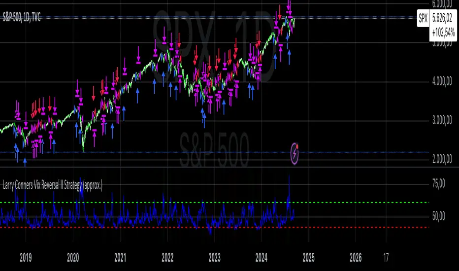
JordanSwindenLibraryLibrary "JordanSwindenLibrary"
TODO: add library description here
getDecimals()
Calculates how many decimals are on the quote price of the current market
Returns: The current decimal places on the market quote price
getPipSize(multiplier)
Calculates the pip size of the current market
Parameters:
multiplier (int) : The mintick point multiplier (1 by default, 10 for FX/Crypto/CFD but can be used to override when certain markets require)
Returns: The pip size for the current market
truncate(number, decimalPlaces)
Truncates (cuts) excess decimal places
Parameters:
number (float) : The number to truncate
decimalPlaces (simple float) : (default=2) The number of decimal places to truncate to
Returns: The given number truncated to the given decimalPlaces
toWhole(number)
Converts pips into whole numbers
Parameters:
number (float) : The pip number to convert into a whole number
Returns: The converted number
toPips(number)
Converts whole numbers back into pips
Parameters:
number (float) : The whole number to convert into pips
Returns: The converted number
getPctChange(value1, value2, lookback)
Gets the percentage change between 2 float values over a given lookback period
Parameters:
value1 (float) : The first value to reference
value2 (float) : The second value to reference
lookback (int) : The lookback period to analyze
Returns: The percent change over the two values and lookback period
random(minRange, maxRange)
Wichmann–Hill Pseudo-Random Number Generator
Parameters:
minRange (float) : The smallest possible number (default: 0)
maxRange (float) : The largest possible number (default: 1)
Returns: A random number between minRange and maxRange
bullFib(priceLow, priceHigh, fibRatio)
Calculates a bullish fibonacci value
Parameters:
priceLow (float) : The lowest price point
priceHigh (float) : The highest price point
fibRatio (float) : The fibonacci % ratio to calculate
Returns: The fibonacci value of the given ratio between the two price points
bearFib(priceLow, priceHigh, fibRatio)
Calculates a bearish fibonacci value
Parameters:
priceLow (float) : The lowest price point
priceHigh (float) : The highest price point
fibRatio (float) : The fibonacci % ratio to calculate
Returns: The fibonacci value of the given ratio between the two price points
getMA(length, maType)
Gets a Moving Average based on type (! MUST BE CALLED ON EVERY TICK TO BE ACCURATE, don't place in scopes)
Parameters:
length (simple int) : The MA period
maType (string) : The type of MA
Returns: A moving average with the given parameters
barsAboveMA(lookback, ma)
Counts how many candles are above the MA
Parameters:
lookback (int) : The lookback period to look back over
ma (float) : The moving average to check
Returns: The bar count of how many recent bars are above the MA
barsBelowMA(lookback, ma)
Counts how many candles are below the MA
Parameters:
lookback (int) : The lookback period to look back over
ma (float) : The moving average to reference
Returns: The bar count of how many recent bars are below the EMA
barsCrossedMA(lookback, ma)
Counts how many times the EMA was crossed recently (based on closing prices)
Parameters:
lookback (int) : The lookback period to look back over
ma (float) : The moving average to reference
Returns: The bar count of how many times price recently crossed the EMA (based on closing prices)
getPullbackBarCount(lookback, direction)
Counts how many green & red bars have printed recently (ie. pullback count)
Parameters:
lookback (int) : The lookback period to look back over
direction (int) : The color of the bar to count (1 = Green, -1 = Red)
Returns: The bar count of how many candles have retraced over the given lookback & direction
getBodySize()
Gets the current candle's body size (in POINTS, divide by 10 to get pips)
Returns: The current candle's body size in POINTS
getTopWickSize()
Gets the current candle's top wick size (in POINTS, divide by 10 to get pips)
Returns: The current candle's top wick size in POINTS
getBottomWickSize()
Gets the current candle's bottom wick size (in POINTS, divide by 10 to get pips)
Returns: The current candle's bottom wick size in POINTS
getBodyPercent()
Gets the current candle's body size as a percentage of its entire size including its wicks
Returns: The current candle's body size percentage
isHammer(fib, colorMatch)
Checks if the current bar is a hammer candle based on the given parameters
Parameters:
fib (float) : (default=0.382) The fib to base candle body on
colorMatch (bool) : (default=false) Does the candle need to be green? (true/false)
Returns: A boolean - true if the current bar matches the requirements of a hammer candle
isStar(fib, colorMatch)
Checks if the current bar is a shooting star candle based on the given parameters
Parameters:
fib (float) : (default=0.382) The fib to base candle body on
colorMatch (bool) : (default=false) Does the candle need to be red? (true/false)
Returns: A boolean - true if the current bar matches the requirements of a shooting star candle
isDoji(wickSize, bodySize)
Checks if the current bar is a doji candle based on the given parameters
Parameters:
wickSize (float) : (default=2) The maximum top wick size compared to the bottom (and vice versa)
bodySize (float) : (default=0.05) The maximum body size as a percentage compared to the entire candle size
Returns: A boolean - true if the current bar matches the requirements of a doji candle
isBullishEC(allowance, rejectionWickSize, engulfWick)
Checks if the current bar is a bullish engulfing candle
Parameters:
allowance (float) : (default=0) How many POINTS to allow the open to be off by (useful for markets with micro gaps)
rejectionWickSize (float) : (default=disabled) The maximum rejection wick size compared to the body as a percentage
engulfWick (bool) : (default=false) Does the engulfing candle require the wick to be engulfed as well?
Returns: A boolean - true if the current bar matches the requirements of a bullish engulfing candle
isBearishEC(allowance, rejectionWickSize, engulfWick)
Checks if the current bar is a bearish engulfing candle
Parameters:
allowance (float) : (default=0) How many POINTS to allow the open to be off by (useful for markets with micro gaps)
rejectionWickSize (float) : (default=disabled) The maximum rejection wick size compared to the body as a percentage
engulfWick (bool) : (default=false) Does the engulfing candle require the wick to be engulfed as well?
Returns: A boolean - true if the current bar matches the requirements of a bearish engulfing candle
isInsideBar()
Detects inside bars
Returns: Returns true if the current bar is an inside bar
isOutsideBar()
Detects outside bars
Returns: Returns true if the current bar is an outside bar
barInSession(sess, useFilter)
Determines if the current price bar falls inside the specified session
Parameters:
sess (simple string) : The session to check
useFilter (bool) : (default=true) Whether or not to actually use this filter
Returns: A boolean - true if the current bar falls within the given time session
barOutSession(sess, useFilter)
Determines if the current price bar falls outside the specified session
Parameters:
sess (simple string) : The session to check
useFilter (bool) : (default=true) Whether or not to actually use this filter
Returns: A boolean - true if the current bar falls outside the given time session
dateFilter(startTime, endTime)
Determines if this bar's time falls within date filter range
Parameters:
startTime (int) : The UNIX date timestamp to begin searching from
endTime (int) : the UNIX date timestamp to stop searching from
Returns: A boolean - true if the current bar falls within the given dates
dayFilter(monday, tuesday, wednesday, thursday, friday, saturday, sunday)
Checks if the current bar's day is in the list of given days to analyze
Parameters:
monday (bool) : Should the script analyze this day? (true/false)
tuesday (bool) : Should the script analyze this day? (true/false)
wednesday (bool) : Should the script analyze this day? (true/false)
thursday (bool) : Should the script analyze this day? (true/false)
friday (bool) : Should the script analyze this day? (true/false)
saturday (bool) : Should the script analyze this day? (true/false)
sunday (bool) : Should the script analyze this day? (true/false)
Returns: A boolean - true if the current bar's day is one of the given days
atrFilter(atrValue, maxSize)
Parameters:
atrValue (float)
maxSize (float)
tradeCount()
Calculate total trade count
Returns: Total closed trade count
isLong()
Check if we're currently in a long trade
Returns: True if our position size is positive
isShort()
Check if we're currently in a short trade
Returns: True if our position size is negative
isFlat()
Check if we're currentlyflat
Returns: True if our position size is zero
wonTrade()
Check if this bar falls after a winning trade
Returns: True if we just won a trade
lostTrade()
Check if this bar falls after a losing trade
Returns: True if we just lost a trade
maxDrawdownRealized()
Gets the max drawdown based on closed trades (ie. realized P&L). The strategy tester displays max drawdown as open P&L (unrealized).
Returns: The max drawdown based on closed trades (ie. realized P&L). The strategy tester displays max drawdown as open P&L (unrealized).
totalPipReturn()
Gets the total amount of pips won/lost (as a whole number)
Returns: Total amount of pips won/lost (as a whole number)
longWinCount()
Count how many winning long trades we've had
Returns: Long win count
shortWinCount()
Count how many winning short trades we've had
Returns: Short win count
longLossCount()
Count how many losing long trades we've had
Returns: Long loss count
shortLossCount()
Count how many losing short trades we've had
Returns: Short loss count
breakEvenCount(allowanceTicks)
Count how many break-even trades we've had
Parameters:
allowanceTicks (float) : Optional - how many ticks to allow between entry & exit price (default 0)
Returns: Break-even count
longCount()
Count how many long trades we've taken
Returns: Long trade count
shortCount()
Count how many short trades we've taken
Returns: Short trade count
longWinPercent()
Calculate win rate of long trades
Returns: Long win rate (0-100)
shortWinPercent()
Calculate win rate of short trades
Returns: Short win rate (0-100)
breakEvenPercent(allowanceTicks)
Calculate break even rate of all trades
Parameters:
allowanceTicks (float) : Optional - how many ticks to allow between entry & exit price (default 0)
Returns: Break-even win rate (0-100)
averageRR()
Calculate average risk:reward
Returns: Average winning trade divided by average losing trade
unitsToLots(units)
(Forex) Convert the given unit count to lots (multiples of 100,000)
Parameters:
units (float) : The units to convert into lots
Returns: Units converted to nearest lot size (as float)
getFxPositionSize(balance, risk, stopLossPips, fxRate, lots)
(Forex) Calculate fixed-fractional position size based on given parameters
Parameters:
balance (float) : The account balance
risk (float) : The % risk (whole number)
stopLossPips (float) : Pip distance to base risk on
fxRate (float) : The conversion currency rate (more info below in library documentation)
lots (bool) : Whether or not to return the position size in lots rather than units (true by default)
Returns: Units/lots to enter into "qty=" parameter of strategy entry function
EXAMPLE USAGE:
string conversionCurrencyPair = (strategy.account_currency == syminfo.currency ? syminfo.tickerid : strategy.account_currency + syminfo.currency)
float fx_rate = request.security(conversionCurrencyPair, timeframe.period, close )
if (longCondition)
strategy.entry("Long", strategy.long, qty=zen.getFxPositionSize(strategy.equity, 1, stopLossPipsWholeNumber, fx_rate, true))
skipTradeMonteCarlo(chance, debug)
Checks to see if trade should be skipped to emulate rudimentary Monte Carlo simulation
Parameters:
chance (float) : The chance to skip a trade (0-1 or 0-100, function will normalize to 0-1)
debug (bool) : Whether or not to display a label informing of the trade skip
Returns: True if the trade is skipped, false if it's not skipped (idea being to include this function in entry condition validation checks)
fillCell(tableID, column, row, title, value, bgcolor, txtcolor, tooltip)
This updates the given table's cell with the given values
Parameters:
tableID (table) : The table ID to update
column (int) : The column to update
row (int) : The row to update
title (string) : The title of this cell
value (string) : The value of this cell
bgcolor (color) : The background color of this cell
txtcolor (color) : The text color of this cell
tooltip (string)
Returns: Nothing.

Larry Connors 3 Day High/Low StrategyThe Larry Connors 3 Day High/Low Strategy is a short-term mean-reversion trading strategy that is designed to identify potential buying opportunities when a security is oversold. This strategy is based on the principles developed by Larry Connors, a well-known trading system developer and author.
Key Strategy Elements:
1. Trend Confirmation: The strategy first confirms that the security is in a long-term uptrend by ensuring that the closing price is above the 200-day moving average (condition1). This rule helps filter trades to align with the longer-term trend.
2. Short-Term Pullback: The strategy looks for a short-term pullback by ensuring that the closing price is below the 5-day moving average (condition2). This identifies potential entry points when the price temporarily moves against the longer-term trend.
3. Three Consecutive Lower Highs and Lows:
• The high and low two days ago are lower than those of the day before (condition3).
• The high and low yesterday are lower than those of two days ago (condition4).
• Today’s high and low are lower than yesterday’s (condition5).
These conditions are used to identify a sequence of declining highs and lows, signaling a short-term pullback or oversold condition in the context of an overall uptrend.
4. Entry and Exit Signals:
• Buy Signal: A buy order is triggered when all the above conditions are met (buyCondition).
• Sell Signal: A sell order is executed when the closing price is above the 5-day moving average (sellCondition), indicating that the pullback might be ending.
Risks of the Strategy
1. Mean Reversion Failure: This strategy relies on the assumption that prices will revert to the mean after a short-term pullback. In strong downtrends or during market crashes, prices may continue to decline, leading to significant losses.
2. Whipsaws and False Signals: The strategy may generate false signals, especially in choppy or sideways markets where the price does not follow a clear trend. This can lead to frequent small losses that can add up over time.
3. Dependence on Historical Patterns: The strategy is based on historical price patterns, which do not always predict future price movements accurately. Sudden market news or economic changes can disrupt the pattern.
4. Lack of Risk Management: The strategy as written does not include stop losses or position sizing rules, which can expose traders to larger-than-expected losses if conditions change rapidly.
About Larry Connors
Larry Connors is a renowned trader, author, and founder of Connors Research and TradingMarkets.com. He is widely recognized for his development of quantitative trading strategies, especially those focusing on short-term mean reversion techniques. Connors has authored several books on trading, including “Short-Term Trading Strategies That Work” and “Street Smarts,” co-authored with Linda Raschke. His strategies are known for their systematic, rules-based approach and have been widely used by traders and investment professionals.
Connors’ research often emphasizes the importance of trading with the trend, managing risk, and using statistically validated techniques to improve trading outcomes. His work has been influential in the field of quantitative trading, providing accessible strategies for traders at various skill levels.
References
1. Connors, L., & Raschke, L. (1995). Street Smarts: High Probability Short-Term Trading Strategies.
2. Connors, L. (2009). Short-Term Trading Strategies That Work.
3. Fama, E. F., & French, K. R. (1988). Permanent and Temporary Components of Stock Prices. Journal of Political Economy, 96(2), 246-273.
This strategy and its variations are popular among traders looking to capitalize on short-term price movements while aligning with longer-term trends. However, like all trading strategies, it requires rigorous backtesting and risk management to ensure its effectiveness under different market conditions.
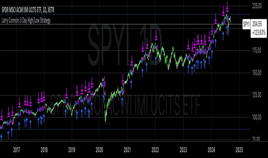
RSI Trend Following StrategyOverview
The RSI Trend Following Strategy utilizes Relative Strength Index (RSI) to enter the trade for the potential trend continuation. It uses Stochastic indicator to check is the price is not in overbought territory and the MACD to measure the current price momentum. Moreover, it uses the 200-period EMA to filter the counter trend trades with the higher probability. The strategy opens only long trades.
Unique Features
Dynamic stop-loss system: Instead of fixed stop-loss level strategy utilizes average true range (ATR) multiplied by user given number subtracted from the position entry price as a dynamic stop loss level.
Configurable Trading Periods: Users can tailor the strategy to specific market windows, adapting to different market conditions.
Two layers trade filtering system: Strategy utilizes MACD and Stochastic indicators measure the current momentum and overbought condition and use 200-period EMA to filter trades against major trend.
Trailing take profit level: After reaching the trailing profit activation level script activates the trailing of long trade using EMA. More information in methodology.
Wide opportunities for strategy optimization: Flexible strategy settings allows users to optimize the strategy entries and exits for chosen trading pair and time frame.
Methodology
The strategy opens long trade when the following price met the conditions:
RSI is above 50 level.
MACD line shall be above the signal line
Both lines of Stochastic shall be not higher than 80 (overbought territory)
Candle’s low shall be above the 200 period EMA
When long trade is executed, strategy set the stop-loss level at the price ATR multiplied by user-given value below the entry price. This level is recalculated on every next candle close, adjusting to the current market volatility.
At the same time strategy set up the trailing stop validation level. When the price crosses the level equals entry price plus ATR multiplied by user-given value script starts to trail the price with trailing EMA(by default = 20 period). If price closes below EMA long trade is closed. When the trailing starts, script prints the label “Trailing Activated”.
Strategy settings
In the inputs window user can setup the following strategy settings:
ATR Stop Loss (by default = 1.75)
ATR Trailing Profit Activation Level (by default = 2.25)
MACD Fast Length (by default = 12, period of averaging fast MACD line)
MACD Fast Length (by default = 26, period of averaging slow MACD line)
MACD Signal Smoothing (by default = 9, period of smoothing MACD signal line)
Oscillator MA Type (by default = EMA, available options: SMA, EMA)
Signal Line MA Type (by default = EMA, available options: SMA, EMA)
RSI Length (by default = 14, period for RSI calculation)
Trailing EMA Length (by default = 20, period for EMA, which shall be broken close the trade after trailing profit activation)
Justification of Methodology
This trading strategy is designed to leverage a combination of technical indicators—Relative Strength Index (RSI), Moving Average Convergence Divergence (MACD), Stochastic Oscillator, and the 200-period Exponential Moving Average (EMA)—to determine optimal entry points for long trades. Additionally, the strategy uses the Average True Range (ATR) for dynamic risk management to adapt to varying market conditions. Let's look in details for which purpose each indicator is used for and why it is used in this combination.
Relative Strength Index (RSI) is a momentum indicator used in technical analysis to measure the speed and change of price movements in a financial market. It helps traders identify whether an asset is potentially overbought (overvalued) or oversold (undervalued), which can indicate a potential reversal or continuation of the current trend.
How RSI Works? RSI tracks the strength of recent price changes. It compares the average gains and losses over a specific period (usually 14 periods) to assess the momentum of an asset. Average gain is the average of all positive price changes over the chosen period. It reflects how much the price has typically increased during upward movements. Average loss is the average of all negative price changes over the same period. It reflects how much the price has typically decreased during downward movements.
RSI calculates these average gains and losses and compares them to create a value between 0 and 100. If the RSI value is above 70, the asset is generally considered overbought, meaning it might be due for a price correction or reversal downward. Conversely, if the RSI value is below 30, the asset is considered oversold, suggesting it could be poised for an upward reversal or recovery. RSI is a useful tool for traders to determine market conditions and make informed decisions about entering or exiting trades based on the perceived strength or weakness of an asset's price movements.
This strategy uses RSI as a short-term trend approximation. If RSI crosses over 50 it means that there is a high probability of short-term trend change from downtrend to uptrend. Therefore RSI above 50 is our first trend filter to look for a long position.
The MACD (Moving Average Convergence Divergence) is a popular momentum and trend-following indicator used in technical analysis. It helps traders identify changes in the strength, direction, momentum, and duration of a trend in an asset's price.
The MACD consists of three components:
MACD Line: This is the difference between a short-term Exponential Moving Average (EMA) and a long-term EMA, typically calculated as: MACD Line = 12 period EMA − 26 period EMA
Signal Line: This is a 9-period EMA of the MACD Line, which helps to identify buy or sell signals. When the MACD Line crosses above the Signal Line, it can be a bullish signal (suggesting a buy); when it crosses below, it can be a bearish signal (suggesting a sell).
Histogram: The histogram shows the difference between the MACD Line and the Signal Line, visually representing the momentum of the trend. Positive histogram values indicate increasing bullish momentum, while negative values indicate increasing bearish momentum.
This strategy uses MACD as a second short-term trend filter. When MACD line crossed over the signal line there is a high probability that uptrend has been started. Therefore MACD line above signal line is our additional short-term trend filter. In conjunction with RSI it decreases probability of following false trend change signals.
The Stochastic Indicator is a momentum oscillator that compares a security's closing price to its price range over a specific period. It's used to identify overbought and oversold conditions. The indicator ranges from 0 to 100, with readings above 80 indicating overbought conditions and readings below 20 indicating oversold conditions.
It consists of two lines:
%K: The main line, calculated using the formula (CurrentClose−LowestLow)/(HighestHigh−LowestLow)×100 . Highest and lowest price taken for 14 periods.
%D: A smoothed moving average of %K, often used as a signal line.
This strategy uses stochastic to define the overbought conditions. The logic here is the following: we want to avoid long trades in the overbought territory, because when indicator reaches it there is a high probability that the potential move is gonna be restricted.
The 200-period EMA is a widely recognized indicator for identifying the long-term trend direction. The strategy only trades in the direction of this primary trend to increase the probability of successful trades. For instance, when the price is above the 200 EMA, only long trades are considered, aligning with the overarching trend direction.
Therefore, strategy uses combination of RSI and MACD to increase the probability that price now is in short-term uptrend, Stochastic helps to avoid the trades in the overbought (>80) territory. To increase the probability of opening long trades in the direction of a main trend and avoid local bounces we use 200 period EMA.
ATR is used to adjust the strategy risk management to the current market volatility. If volatility is low, we don’t need the large stop loss to understand the there is a high probability that we made a mistake opening the trade. User can setup the settings ATR Stop Loss and ATR Trailing Profit Activation Level to realize his own risk to reward preferences, but the unique feature of a strategy is that after reaching trailing profit activation level strategy is trying to follow the trend until it is likely to be finished instead of using fixed risk management settings. It allows sometimes to be involved in the large movements.
Backtest Results
Operating window: Date range of backtests is 2023.01.01 - 2024.08.01. It is chosen to let the strategy to close all opened positions.
Commission and Slippage: Includes a standard Binance commission of 0.1% and accounts for possible slippage over 5 ticks.
Initial capital: 10000 USDT
Percent of capital used in every trade: 30%
Maximum Single Position Loss: -3.94%
Maximum Single Profit: +15.78%
Net Profit: +1359.21 USDT (+13.59%)
Total Trades: 111 (36.04% win rate)
Profit Factor: 1.413
Maximum Accumulated Loss: 625.02 USDT (-5.85%)
Average Profit per Trade: 12.25 USDT (+0.40%)
Average Trade Duration: 40 hours
These results are obtained with realistic parameters representing trading conditions observed at major exchanges such as Binance and with realistic trading portfolio usage parameters.
How to Use
Add the script to favorites for easy access.
Apply to the desired timeframe and chart (optimal performance observed on 2h BTC/USDT).
Configure settings using the dropdown choice list in the built-in menu.
Set up alerts to automate strategy positions through web hook with the text: {{strategy.order.alert_message}}
Disclaimer:
Educational and informational tool reflecting Skyrex commitment to informed trading. Past performance does not guarantee future results. Test strategies in a simulated environment before live implementation
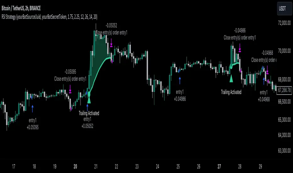
Intramarket Difference Index StrategyHi Traders !!
The IDI Strategy:
In layman’s terms this strategy compares two indicators across markets and exploits their differences.
note: it is best the two markets are correlated as then we know we are trading a short to long term deviation from both markets' general trend with the assumption both markets will trend again sometime in the future thereby exhausting our trading opportunity.
📍 Import Notes:
This Strategy calculates trade position size independently (i.e. risk per trade is controlled in the user inputs tab), this means that the ‘Order size’ input in the ‘Properties’ tab will have no effect on the strategy. Why ? because this allows us to define custom position size algorithms which we can use to improve our risk management and equity growth over time. Here we have the option to have fixed quantity or fixed percentage of equity ATR (Average True Range) based stops in addition to the turtle trading position size algorithm.
‘Pyramiding’ does not work for this strategy’, similar to the order size input togeling this input will have no effect on the strategy as the strategy explicitly defines the maximum order size to be 1.
This strategy is not perfect, and as of writing of this post I have not traded this algo.
Always take your time to backtests and debug the strategy.
🔷 The IDI Strategy:
By default this strategy pulls data from your current TV chart and then compares it to the base market, be default BINANCE:BTCUSD . The strategy pulls SMA and RSI data from either market (we call this the difference data), standardizes the data (solving the different unit problem across markets) such that it is comparable and then differentiates the data, calling the result of this transformation and difference the Intramarket Difference (ID). The formula for the the ID is
ID = market1_diff_data - market2_diff_data (1)
Where
market(i)_diff_data = diff_data / ATR(j)_market(i)^0.5,
where i = {1, 2} and j = the natural numbers excluding 0
Formula (1) interpretation is the following
When ID > 0: this means the current market outperforms the base market
When ID = 0: Markets are at long run equilibrium
When ID < 0: this means the current market underperforms the base market
To form the strategy we define one of two strategy type’s which are Trend and Mean Revesion respectively.
🔸 Trend Case:
Given the ‘‘Strategy Type’’ is equal to TREND we define a threshold for which if the ID crosses over we go long and if the ID crosses under the negative of the threshold we go short.
The motivating idea is that the ID is an indicator of the two symbols being out of sync, and given we know volatility clustering, momentum and mean reversion of anomalies to be a stylised fact of financial data we can construct a trading premise. Let's first talk more about this premise.
For some markets (cryptocurrency markets - synthetic symbols in TV) the stylised fact of momentum is true, this means that higher momentum is followed by higher momentum, and given we know momentum to be a vector quantity (with magnitude and direction) this momentum can be both positive and negative i.e. when the ID crosses above some threshold we make an assumption it will continue in that direction for some time before executing back to its long run equilibrium of 0 which is a reasonable assumption to make if the market are correlated. For example for the BTCUSD - ETHUSD pair, if the ID > +threshold (inputs for MA and RSI based ID thresholds are found under the ‘‘INTRAMARKET DIFFERENCE INDEX’’ group’), ETHUSD outperforms BTCUSD, we assume the momentum to continue so we go long ETHUSD.
In the standard case we would exit the market when the IDI returns to its long run equilibrium of 0 (for the positive case the ID may return to 0 because ETH’s difference data may have decreased or BTC’s difference data may have increased). However in this strategy we will not define this as our exit condition, why ?
This is because we want to ‘‘let our winners run’’, to achieve this we define a trailing Donchian Channel stop loss (along with a fixed ATR based stop as our volatility proxy). If we were too use the 0 exit the strategy may print a buy signal (ID > +threshold in the simple case, market regimes may be used), return to 0 and then print another buy signal, and this process can loop may times, this high trade frequency means we fail capture the entire market move lowering our profit, furthermore on lower time frames this high trade frequencies mean we pay more transaction costs (due to price slippage, commission and big-ask spread) which means less profit.
By capturing the sum of many momentum moves we are essentially following the trend hence the trend following strategy type.
Here we also print the IDI (with default strategy settings with the MA difference type), we can see that by letting our winners run we may catch many valid momentum moves, that results in a larger final pnl that if we would otherwise exit based on the equilibrium condition(Valid trades are denoted by solid green and red arrows respectively and all other valid trades which occur within the original signal are light green and red small arrows).
another example...
Note: if you would like to plot the IDI separately copy and paste the following code in a new Pine Script indicator template.
indicator("IDI")
// INTRAMARKET INDEX
var string g_idi = "intramarket diffirence index"
ui_index_1 = input.symbol("BINANCE:BTCUSD", title = "Base market", group = g_idi)
// ui_index_2 = input.symbol("BINANCE:ETHUSD", title = "Quote Market", group = g_idi)
type = input.string("MA", title = "Differrencing Series", options = , group = g_idi)
ui_ma_lkb = input.int(24, title = "lookback of ma and volatility scaling constant", group = g_idi)
ui_rsi_lkb = input.int(14, title = "Lookback of RSI", group = g_idi)
ui_atr_lkb = input.int(300, title = "ATR lookback - Normalising value", group = g_idi)
ui_ma_threshold = input.float(5, title = "Threshold of Upward/Downward Trend (MA)", group = g_idi)
ui_rsi_threshold = input.float(20, title = "Threshold of Upward/Downward Trend (RSI)", group = g_idi)
//>>+----------------------------------------------------------------+}
// CUSTOM FUNCTIONS |
//<<+----------------------------------------------------------------+{
// construct UDT (User defined type) containing the IDI (Intramarket Difference Index) source values
// UDT will hold many variables / functions grouped under the UDT
type functions
float Close // close price
float ma // ma of symbol
float rsi // rsi of the asset
float atr // atr of the asset
// the security data
getUDTdata(symbol, malookback, rsilookback, atrlookback) =>
indexHighTF = barstate.isrealtime ? 1 : 0
= request.security(symbol, timeframe = timeframe.period,
expression = [close , // Instentiate UDT variables
ta.sma(close, malookback) ,
ta.rsi(close, rsilookback) ,
ta.atr(atrlookback) ])
data = functions.new(close_, ma_, rsi_, atr_)
data
// Intramerket Difference Index
idi(type, symbol1, malookback, rsilookback, atrlookback, mathreshold, rsithreshold) =>
threshold = float(na)
index1 = getUDTdata(symbol1, malookback, rsilookback, atrlookback)
index2 = getUDTdata(syminfo.tickerid, malookback, rsilookback, atrlookback)
// declare difference variables for both base and quote symbols, conditional on which difference type is selected
var diffindex1 = 0.0, var diffindex2 = 0.0,
// declare Intramarket Difference Index based on series type, note
// if > 0, index 2 outpreforms index 1, buy index 2 (momentum based) until equalibrium
// if < 0, index 2 underpreforms index 1, sell index 1 (momentum based) until equalibrium
// for idi to be valid both series must be stationary and normalised so both series hae he same scale
intramarket_difference = 0.0
if type == "MA"
threshold := mathreshold
diffindex1 := (index1.Close - index1.ma) / math.pow(index1.atr*malookback, 0.5)
diffindex2 := (index2.Close - index2.ma) / math.pow(index2.atr*malookback, 0.5)
intramarket_difference := diffindex2 - diffindex1
else if type == "RSI"
threshold := rsilookback
diffindex1 := index1.rsi
diffindex2 := index2.rsi
intramarket_difference := diffindex2 - diffindex1
//>>+----------------------------------------------------------------+}
// STRATEGY FUNCTIONS CALLS |
//<<+----------------------------------------------------------------+{
// plot the intramarket difference
= idi(type,
ui_index_1,
ui_ma_lkb,
ui_rsi_lkb,
ui_atr_lkb,
ui_ma_threshold,
ui_rsi_threshold)
//>>+----------------------------------------------------------------+}
plot(intramarket_difference, color = color.orange)
hline(type == "MA" ? ui_ma_threshold : ui_rsi_threshold, color = color.green)
hline(type == "MA" ? -ui_ma_threshold : -ui_rsi_threshold, color = color.red)
hline(0)
Note it is possible that after printing a buy the strategy then prints many sell signals before returning to a buy, which again has the same implication (less profit. Potentially because we exit early only for price to continue upwards hence missing the larger "trend"). The image below showcases this cenario and again, by allowing our winner to run we may capture more profit (theoretically).
This should be clear...
🔸 Mean Reversion Case:
We stated prior that mean reversion of anomalies is an standerdies fact of financial data, how can we exploit this ?
We exploit this by normalizing the ID by applying the Ehlers fisher transformation. The transformed data is then assumed to be approximately normally distributed. To form the strategy we employ the same logic as for the z score, if the FT normalized ID > 2.5 (< -2.5) we buy (short). Our exit conditions remain unchanged (fixed ATR stop and trailing Donchian Trailing stop)
🔷 Position Sizing:
If ‘‘Fixed Risk From Initial Balance’’ is toggled true this means we risk a fixed percentage of our initial balance, if false we risk a fixed percentage of our equity (current balance).
Note we also employ a volatility adjusted position sizing formula, the turtle training method which is defined as follows.
Turtle position size = (1/ r * ATR * DV) * C
Where,
r = risk factor coefficient (default is 20)
ATR(j) = risk proxy, over j times steps
DV = Dollar Volatility, where DV = (1/Asset Price) * Capital at Risk
🔷 Risk Management:
Correct money management means we can limit risk and increase reward (theoretically). Here we employ
Max loss and gain per day
Max loss per trade
Max number of consecutive losing trades until trade skip
To read more see the tooltips (info circle).
🔷 Take Profit:
By defualt the script uses a Donchain Channel as a trailing stop and take profit, In addition to this the script defines a fixed ATR stop losses (by defualt, this covers cases where the DC range may be to wide making a fixed ATR stop usefull), ATR take profits however are defined but optional.
ATR SL and TP defined for all trades
🔷 Hurst Regime (Regime Filter):
The Hurst Exponent (H) aims to segment the market into three different states, Trending (H > 0.5), Random Geometric Brownian Motion (H = 0.5) and Mean Reverting / Contrarian (H < 0.5). In my interpretation this can be used as a trend filter that eliminates market noise.
We utilize the trending and mean reverting based states, as extra conditions required for valid trades for both strategy types respectively, in the process increasing our trade entry quality.
🔷 Example model Architecture:
Here is an example of one configuration of this strategy, combining all aspects discussed in this post.
Future Updates
- Automation integration (next update)
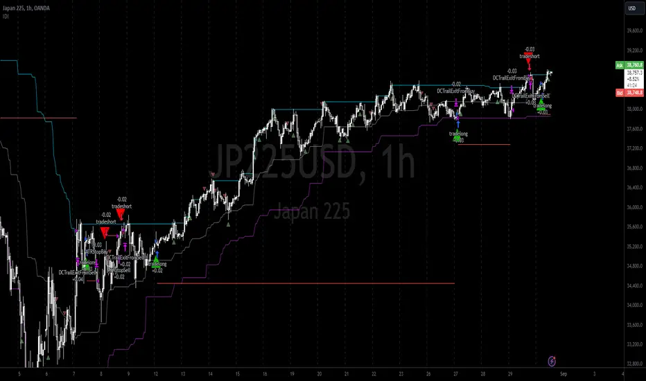
Gann + Laplace Smoothed Hybrid Volume Spread AnalysisThe Gann + Laplace Smoothed Hybrid Volume Spread Analysis ( GannLSHVSA ) Strategy/Indicator is an trading tool designed to fuse volume analysis with trend detection, offering traders a view of market dynamics.
This Strategy/Indicator stands apart by integrating the principles of the upgraded Discrete Fourier Transform (DFT), the Laplace Stieltjes Transform and volume spread analysis, enhanced with a layer of Fourier smoothing to distill market noise and highlight trend directions with unprecedented clarity.
The length of EMA and Strategy Entries are modified with the Gann swings .
This smoothing process allows traders to discern the true underlying patterns in volume and price action, stripped of the distractions of short-term fluctuations and noise.
The core functionality of the GannLSHVSA revolves around the innovative combination of volume change analysis, spread determination (calculated from the open and close price difference), and the strategic use of the EMA (default 10) to fine-tune the analysis of spread by incorporating volume changes.
Trend direction is validated through a moving average (MA) of the histogram, which acts analogously to the Volume MA found in traditional volume indicators. This MA serves as a pivotal reference point, enabling traders to confidently engage with the market when the histogram's movement concurs with the trend direction, particularly when it crosses the Trend MA line, signalling optimal entry points.
It returns 0 when MA of the histogram and EMA of the Price Spread are not align.
WHAT IS GannLSHVSA INDICATOR:
The GannLSHVSA plots a positive trend when a positive Volume smoothed Spread and EMA of Volume smoothed price is above 0, and a negative when negative Volume smoothed Spread and EMA of Volume smoothed price is below 0. When this conditions are not met it plots 0.
HOW TO USE THE STRATEGY:
Here you fine-tune the inputs until you find a combination that works well on all Timeframes you will use when creating your Automated Trade Algorithmic Strategy. I suggest 4h, 12h, 1D, 2D, 3D, 4D, 5D, 6D, W and M.
ORIGINALITY & USEFULNESS:
The GannLSHVSA Strategy is unique because it applies upgraded DFT, the Laplace Stieltjes Transform for data smoothing, effectively filtering out the minor fluctuations and leaving traders with a clear picture of the market's true movements. The DFT's ability to break down market signals into constituent frequencies offers a granular view of market dynamics, highlighting the amplitude and phase of each frequency component. This, combined with the strategic application of Ehler's Universal Oscillator principles via a histogram, furnishes traders with a nuanced understanding of market volatility and noise levels, thereby facilitating more informed trading decisions. The Gann swing strategy is developed by meomeo105, this Gann high and low algorithm forms the basis of the EMA modification.
DETAILED DESCRIPTION:
My detailed description of the indicator and use cases which I find very valuable.
What is the meaning of price spread?
In finance, a spread refers to the difference between two prices, rates, or yields. One of the most common types is the bid-ask spread, which refers to the gap between the bid (from buyers) and the ask (from sellers) prices of a security or asset.
We are going to use Open-Close spread.
What is Volume spread analysis?
Volume spread analysis (VSA) is a method of technical analysis that compares the volume per candle, range spread, and closing price to determine price direction.
What does this mean?
We need to have a positive Volume Price Spread and a positive Moving average of Volume price spread for a positive trend. OR via versa a negative Volume Price Spread and a negative Moving average of Volume price spread for a negative trend.
What if we have a positive Volume Price Spread and a negative Moving average of Volume Price Spread?
It results in a neutral, not trending price action.
Thus the Indicator/Strategy returns 0 and Closes all long and short positions.
I suggest using "Close all" input False when fine-tuning Inputs for 1 TimeFrame. When you export data to Excel/Numbers/GSheets I suggest using "Close all" input as True, except for the lowest TimeFrame. I suggest using 100% equity as your default quantity for fine-tune purposes. I have to mention that 100% equity may lead to unrealistic backtesting results. Be avare. When backtesting for trading purposes use Contracts or USDT.
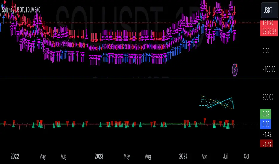
MACD with 1D Stochastic Confirmation Reversal StrategyOverview
The MACD with 1D Stochastic Confirmation Reversal Strategy utilizes MACD indicator in conjunction with 1 day timeframe Stochastic indicators to obtain the high probability short-term trend reversal signals. The main idea is to wait until MACD line crosses up it’s signal line, at the same time Stochastic indicator on 1D time frame shall show the uptrend (will be discussed in methodology) and not to be in the oversold territory. Strategy works on time frames from 30 min to 4 hours and opens only long trades.
Unique Features
Dynamic stop-loss system: Instead of fixed stop-loss level strategy utilizes average true range (ATR) multiplied by user given number subtracted from the position entry price as a dynamic stop loss level.
Configurable Trading Periods: Users can tailor the strategy to specific market windows, adapting to different market conditions.
Higher time frame confirmation: Strategy utilizes 1D Stochastic to establish the major trend and confirm the local reversals with the higher probability.
Trailing take profit level: After reaching the trailing profit activation level scrip activate the trailing of long trade using EMA. More information in methodology.
Methodology
The strategy opens long trade when the following price met the conditions:
MACD line of MACD indicator shall cross over the signal line of MACD indicator.
1D time frame Stochastic’s K line shall be above the D line.
1D time frame Stochastic’s K line value shall be below 80 (not overbought)
When long trade is executed, strategy set the stop-loss level at the price ATR multiplied by user-given value below the entry price. This level is recalculated on every next candle close, adjusting to the current market volatility.
At the same time strategy set up the trailing stop validation level. When the price crosses the level equals entry price plus ATR multiplied by user-given value script starts to trail the price with EMA. If price closes below EMA long trade is closed. When the trailing starts, script prints the label “Trailing Activated”.
Strategy settings
In the inputs window user can setup the following strategy settings:
ATR Stop Loss (by default = 3.25, value multiplied by ATR to be subtracted from position entry price to setup stop loss)
ATR Trailing Profit Activation Level (by default = 4.25, value multiplied by ATR to be added to position entry price to setup trailing profit activation level)
Trailing EMA Length (by default = 20, period for EMA, when price reached trailing profit activation level EMA will stop out of position if price closes below it)
User can choose the optimal parameters during backtesting on certain price chart, in our example we use default settings.
Justification of Methodology
This strategy leverages 2 time frames analysis to have the high probability reversal setups on lower time frame in the direction of the 1D time frame trend. That’s why it’s recommended to use this strategy on 30 min – 4 hours time frames.
To have an approximation of 1D time frame trend strategy utilizes classical Stochastic indicator. The Stochastic Indicator is a momentum oscillator that compares a security's closing price to its price range over a specific period. It's used to identify overbought and oversold conditions. The indicator ranges from 0 to 100, with readings above 80 indicating overbought conditions and readings below 20 indicating oversold conditions.
It consists of two lines:
%K: The main line, calculated using the formula (CurrentClose−LowestLow)/(HighestHigh−LowestLow)×100 . Highest and lowest price taken for 14 periods.
%D: A smoothed moving average of %K, often used as a signal line.
Strategy logic assumes that on 1D time frame it’s uptrend in %K line is above the %D line. Moreover, we can consider long trade only in %K line is below 80. It means that in overbought state the long trade will not be opened due to higher probability of pullback or even major trend reversal. If these conditions are met we are going to our working (lower) time frame.
On the chosen time frame, we remind you that for correct work of this strategy you shall use 30min – 4h time frames, MACD line shall cross over it’s signal line. The MACD (Moving Average Convergence Divergence) is a popular momentum and trend-following indicator used in technical analysis. It helps traders identify changes in the strength, direction, momentum, and duration of a trend in a stock's price.
The MACD consists of three components:
MACD Line: This is the difference between a short-term Exponential Moving Average (EMA) and a long-term EMA, typically calculated as: MACD Line=12-period EMA−26-period
Signal Line: This is a 9-period EMA of the MACD Line, which helps to identify buy or sell signals. When the MACD Line crosses above the Signal Line, it can be a bullish signal (suggesting a buy); when it crosses below, it can be a bearish signal (suggesting a sell).
Histogram: The histogram shows the difference between the MACD Line and the Signal Line, visually representing the momentum of the trend. Positive histogram values indicate increasing bullish momentum, while negative values indicate increasing bearish momentum.
In our script we are interested in only MACD and signal lines. When MACD line crosses signal line there is a high chance that short-term trend reversed to the upside. We use this strategy on 45 min time frame.
ATR is used to adjust the strategy risk management to the current market volatility. If volatility is low, we don’t need the large stop loss to understand the there is a high probability that we made a mistake opening the trade. User can setup the settings ATR Stop Loss and ATR Trailing Profit Activation Level to realize his own risk to reward preferences, but the unique feature of a strategy is that after reaching trailing profit activation level strategy is trying to follow the trend until it is likely to be finished instead of using fixed risk management settings. It allows sometimes to be involved in the large movements.
Backtest Results
Operating window: Date range of backtests is 2023.01.01 - 2024.08.01. It is chosen to let the strategy to close all opened positions.
Commission and Slippage: Includes a standard Binance commission of 0.1% and accounts for possible slippage over 5 ticks.
Initial capital: 10000 USDT
Percent of capital used in every trade: 30%
Maximum Single Position Loss: -4.79%
Maximum Single Profit: +20.14%
Net Profit: +2361.33 USDT (+44.72%)
Total Trades: 123 (44.72% win rate)
Profit Factor: 1.623
Maximum Accumulated Loss: 695.80 USDT (-5.48%)
Average Profit per Trade: 19.20 USDT (+0.59%)
Average Trade Duration: 30 hours
These results are obtained with realistic parameters representing trading conditions observed at major exchanges such as Binance and with realistic trading portfolio usage parameters.
How to Use
Add the script to favorites for easy access.
Apply to the desired timeframe between 30 min and 4 hours and chart (optimal performance observed on 45 min BTC/USDT).
Configure settings using the dropdown choice list in the built-in menu.
Set up alerts to automate strategy positions through web hook with the text: {{strategy.order.alert_message}}
Disclaimer:
Educational and informational tool reflecting Skyrex commitment to informed trading. Past performance does not guarantee future results. Test strategies in a simulated environment before live implementation

Dual Chain StrategyDual Chain Strategy - Technical Overview
How It Works:
The Dual Chain Strategy is a unique approach to trading that utilizes Exponential Moving Averages (EMAs) across different timeframes, creating two distinct "chains" of trading signals. These chains can work independently or together, capturing both long-term trends and short-term price movements.
Chain 1 (Longer-Term Focus):
Entry Signal: The entry signal for Chain 1 is generated when the closing price crosses above the EMA calculated on a weekly timeframe. This suggests the start of a bullish trend and prompts a long position.
bullishChain1 = enableChain1 and ta.crossover(src1, entryEMA1)
Exit Signal: The exit signal is triggered when the closing price crosses below the EMA on a daily timeframe, indicating a potential bearish reversal.
exitLongChain1 = enableChain1 and ta.crossunder(src1, exitEMA1)
Parameters: Chain 1's EMA length is set to 10 periods by default, with the flexibility for user adjustment to match various trading scenarios.
Chain 2 (Shorter-Term Focus):
Entry Signal: Chain 2 generates an entry signal when the closing price crosses above the EMA on a 12-hour timeframe. This setup is designed to capture quicker, shorter-term movements.
bullishChain2 = enableChain2 and ta.crossover(src2, entryEMA2)
Exit Signal: The exit signal occurs when the closing price falls below the EMA on a 9-hour timeframe, indicating the end of the shorter-term trend.
exitLongChain2 = enableChain2 and ta.crossunder(src2, exitEMA2)
Parameters: Chain 2's EMA length is set to 9 periods by default, and can be customized to better align with specific market conditions or trading strategies.
Key Features:
Dual EMA Chains: The strategy's originality shines through its dual-chain configuration, allowing traders to monitor and react to both long-term and short-term market trends. This approach is particularly powerful as it combines the strengths of trend-following with the agility of momentum trading.
Timeframe Flexibility: Users can modify the timeframes for both chains, ensuring the strategy can be tailored to different market conditions and individual trading styles. This flexibility makes it versatile for various assets and trading environments.
Independent Trade Logic: Each chain operates independently, with its own set of entry and exit rules. This allows for simultaneous or separate execution of trades based on the signals from either or both chains, providing a robust trading system that can handle different market phases.
Backtesting Period: The strategy includes a configurable backtesting period, enabling thorough performance assessment over a historical range. This feature is crucial for understanding how the strategy would have performed under different market conditions.
time_cond = time >= startDate and time <= finishDate
What It Does:
The Dual Chain Strategy offers traders a distinctive trading tool that merges two separate EMA-based systems into one cohesive framework. By integrating both long-term and short-term perspectives, the strategy enhances the ability to adapt to changing market conditions. The originality of this script lies in its innovative dual-chain design, providing traders with a unique edge by allowing them to capitalize on both significant trends and smaller, faster price movements.
Whether you aim to capture extended market trends or take advantage of more immediate price action, the Dual Chain Strategy provides a comprehensive solution with a high degree of customization and strategic depth. Its flexibility and originality make it a valuable tool for traders seeking to refine their approach to market analysis and execution.
How to Use the Dual Chain Strategy
Step 1: Access the Strategy
Add the Script: Start by adding the Dual Chain Strategy to your TradingView chart. You can do this by searching for the script by name or using the link provided.
Select the Asset: Apply the strategy to your preferred trading pair or asset, such as #BTCUSD, to see how it performs.
Step 2: Configure the Settings
Enable/Disable Chains:
The strategy is designed with two independent chains. You can choose to enable or disable each chain depending on your trading style and the market conditions.
enableChain1 = input.bool(true, title='Enable Chain 1')
enableChain2 = input.bool(true, title='Enable Chain 2')
By default, both chains are enabled. If you prefer to focus only on longer-term trends, you might disable Chain 2, or vice versa if you prefer shorter-term trades.
Set EMA Lengths:
Adjust the EMA lengths for each chain to match your trading preferences.
Chain 1: The default EMA length is 10 periods. This chain uses a weekly timeframe for entry signals and a daily timeframe for exits.
len1 = input.int(10, minval=1, title='Length Chain 1 EMA', group="Chain 1")
Chain 2: The default EMA length is 9 periods. This chain uses a 12-hour timeframe for entries and a 9-hour timeframe for exits.
len2 = input.int(9, minval=1, title='Length Chain 2 EMA', group="Chain 2")
Customize Timeframes:
You can customize the timeframes used for entry and exit signals for both chains.
Chain 1:
Entry Timeframe: Weekly
Exit Timeframe: Daily
tf1_entry = input.timeframe("W", title='Chain 1 Entry Timeframe', group="Chain 1")
tf1_exit = input.timeframe("D", title='Chain 1 Exit Timeframe', group="Chain 1")
Chain 2:
Entry Timeframe: 12 Hours
Exit Timeframe: 9 Hours
tf2_entry = input.timeframe("720", title='Chain 2 Entry Timeframe (12H)', group="Chain 2")
tf2_exit = input.timeframe("540", title='Chain 2 Exit Timeframe (9H)', group="Chain 2")
Set the Backtesting Period:
Define the period over which you want to backtest the strategy. This allows you to see how the strategy would have performed historically.
startDate = input.time(timestamp('2015-07-27'), title="StartDate")
finishDate = input.time(timestamp('2026-01-01'), title="FinishDate")
Step 3: Analyze the Signals
Understand the Entry and Exit Signals:
Buy Signals: When the price crosses above the entry EMA, the strategy generates a buy signal.
bullishChain1 = enableChain1 and ta.crossover(src1, entryEMA1)
Sell Signals: When the price crosses below the exit EMA, the strategy generates a sell signal.
bearishChain2 = enableChain2 and ta.crossunder(src2, entryEMA2)
Review the Visual Indicators:
The strategy plots buy and sell signals on the chart with labels for easy identification:
BUY C1/C2 for buy signals from Chain 1 and Chain 2.
SELL C1/C2 for sell signals from Chain 1 and Chain 2.
This visual aid helps you quickly understand when and why trades are being executed.
Step 4: Optimize the Strategy
Backtest Results:
Review the strategy’s performance over the backtesting period. Look at key metrics like net profit, drawdown, and trade statistics to evaluate its effectiveness.
Adjust the EMA lengths, timeframes, and other settings to see how changes affect the strategy’s performance.
Customize for Live Trading:
Once satisfied with the backtest results, you can apply the strategy settings to live trading. Remember to continuously monitor and adjust as needed based on market conditions.
Step 5: Implement Risk Management
Use Realistic Position Sizing:
Keep your risk exposure per trade within a comfortable range, typically between 1-2% of your trading capital.
Set Alerts:
Set up alerts for buy and sell signals, so you don’t miss trading opportunities.
Paper Trade First:
Consider running the strategy in a paper trading account to understand its behavior in real market conditions before committing real capital.
This dual-layered approach offers a distinct advantage: it enables the strategy to adapt to varying market conditions by capturing both broad trends and immediate price action without one chain's activity impacting the other's decision-making process. The independence of these chains in executing transactions adds a level of sophistication and flexibility that is rarely seen in more conventional trading systems, making the Dual Chain Strategy not just unique, but a powerful tool for traders seeking to navigate complex market environments.
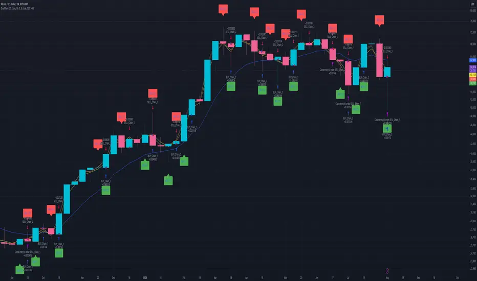
Double CCI Confirmed Hull Moving Average Reversal StrategyOverview
The Double CCI Confirmed Hull Moving Average Strategy utilizes hull moving average (HMA) in conjunction with two commodity channel index (CCI) indicators: the slow and fast to increase the probability of entering when the short and mid-term uptrend confirmed. The main idea is to wait until the price breaks the HMA while both CCI are showing that the uptrend has likely been already started. Moreover, strategy uses exponential moving average (EMA) to trail the price when it reaches the specific level. The strategy opens only long trades.
Unique Features
Dynamic stop-loss system: Instead of fixed stop-loss level strategy utilizes average true range (ATR) multiplied by user given number subtracted from the position entry price as a dynamic stop loss level.
Configurable Trading Periods: Users can tailor the strategy to specific market windows, adapting to different market conditions.
Double trade setup confirmation: Strategy utilizes two different period CCI indicators to confirm the breakouts of HMA.
Trailing take profit level: After reaching the trailing profit activation level scrip activate the trailing of long trade using EMA. More information in methodology.
Methodology
The strategy opens long trade when the following price met the conditions:
Short-term period CCI indicator shall be above 0.
Long-term period CCI indicator shall be above 0.
Price shall cross the HMA and candle close above it with the same candle
When long trade is executed, strategy set the stop-loss level at the price ATR multiplied by user-given value below the entry price. This level is recalculated on every next candle close, adjusting to the current market volatility.
At the same time strategy set up the trailing stop validation level. When the price crosses the level equals entry price plus ATR multiplied by user-given value script starts to trail the price with EMA. If price closes below EMA long trade is closed. When the trailing starts, script prints the label “Trailing Activated”.
Strategy settings
In the inputs window user can setup the following strategy settings:
ATR Stop Loss (by default = 1.75)
ATR Trailing Profit Activation Level (by default = 2.25)
CCI Fast Length (by default = 25, used for calculation short term period CCI
CCI Slow Length (by default = 50, used for calculation long term period CCI)
Hull MA Length (by default = 34, period of HMA, which shall be broken to open trade)
Trailing EMA Length (by default = 20)
User can choose the optimal parameters during backtesting on certain price chart.
Justification of Methodology
Before understanding why this particular combination of indicator has been chosen let's briefly explain what is CCI and HMA.
The Commodity Channel Index (CCI) is a momentum-based technical indicator used in trading to measure a security's price relative to its average price over a given period. Developed by Donald Lambert in 1980, the CCI is primarily used to identify cyclical trends in a security, helping traders to spot potential buying or selling opportunities.
The CCI formula is:
CCI = (Typical Price − SMA) / (0.015 × Mean Deviation)
Typical Price (TP): This is calculated as the average of the high, low, and closing prices for the period.
Simple Moving Average (SMA): This is the average of the Typical Prices over a specific number of periods.
Mean Deviation: This is the average of the absolute differences between the Typical Price and the SMA.
The result is a value that typically fluctuates between +100 and -100, though it is not bounded and can go higher or lower depending on the price movement.
The Hull Moving Average (HMA) is a type of moving average that was developed by Alan Hull to improve upon the traditional moving averages by reducing lag while maintaining smoothness. The goal of the HMA is to create an indicator that is both quick to respond to price changes and less prone to whipsaws (false signals).
How the Hull Moving Average is Calculated?
The Hull Moving Average is calculated using the following steps:
Weighted Moving Average (WMA): The HMA starts by calculating the Weighted Moving Average (WMA) of the price data over a period square root of n (sqrt(n))
Speed Adjustment: A WMA is then calculated for half of the period n/2, and this is multiplied by 2 to give more weight to recent prices.
Lag Reduction: The WMA of the full period n is subtracted from the doubled n/2 WMA.
Final Smoothing: To smooth the result and reduce noise, a WMA is calculated for the square root of the period n.
The formula can be represented as:
HMA(n) = WMA(WMA(n/2) × 2 − WMA(n), sqrt(n))
The Weighted Moving Average (WMA) is a type of moving average that gives more weight to recent data points, making it more responsive to recent price changes than a Simple Moving Average (SMA). In a WMA, each data point within the selected period is multiplied by a weight, with the most recent data receiving the highest weight. The sum of these weighted values is then divided by the sum of the weights to produce the WMA.
This strategy leverages HMA of user given period as a critical level which shall be broken to say that probability of trend change to the upside increased. HMA reacts faster than EMA or SMA to the price change, that’s why it increases chances to enter new trade earlier. Long-term period CCI helps to have an approximation of mid-term trend. If it’s above 0 the probability of uptrend increases. Short-period CCI allows to have an approximation of short-term trend reversal from down to uptrend. This approach increases chances to have a long trade setup in the direction of mid-term trend when the short-term trend starts to reverse.
ATR is used to adjust the strategy risk management to the current market volatility. If volatility is low, we don’t need the large stop loss to understand the there is a high probability that we made a mistake opening the trade. User can setup the settings ATR Stop Loss and ATR Trailing Profit Activation Level to realize his own risk to reward preferences, but the unique feature of a strategy is that after reaching trailing profit activation level strategy is trying to follow the trend until it is likely to be finished instead of using fixed risk management settings. It allows sometimes to be involved in the large movements. It’s also important to make a note, that script uses HMA to enter the trade, but for trailing it leverages EMA. It’s used because EMA has no such fast reaction to price move which increases probability not to be stopped out from any significant uptrend move.
Backtest Results
Operating window: Date range of backtests is 2022.07.01 - 2024.08.01. It is chosen to let the strategy to close all opened positions.
Commission and Slippage: Includes a standard Binance commission of 0.1% and accounts for possible slippage over 5 ticks.
Initial capital: 10000 USDT
Percent of capital used in every trade: 100%
Maximum Single Position Loss: -4.67%
Maximum Single Profit: +19.66%
Net Profit: +14897.94 USDT (+148.98%)
Total Trades: 104 (36.54% win rate)
Profit Factor: 2.312
Maximum Accumulated Loss: 1302.66 USDT (-9.58%)
Average Profit per Trade: 143.25 USDT (+0.96%)
Average Trade Duration: 34 hours
These results are obtained with realistic parameters representing trading conditions observed at major exchanges such as Binance and with realistic trading portfolio usage parameters.
How to Use
Add the script to favorites for easy access.
Apply to the desired timeframe and chart (optimal performance observed on 2h BTC/USDT).
Configure settings using the dropdown choice list in the built-in menu.
Set up alerts to automate strategy positions through web hook with the text: {{strategy.order.alert_message}}
Disclaimer:
Educational and informational tool reflecting Skyrex commitment to informed trading. Past performance does not guarantee future results. Test strategies in a simulated environment before live implementation
