eksOr - Charm + Vanna Window (Monthly OPEX)What This Does
This indicator highlights the monthly “Charm + Vanna window” around standard monthly options expiration (the 3rd Friday, i.e., monthly OPEX). It’s a time-based overlay that shades either:
Pre-OPEX: from the first calendar day of the month through the day before OPEX, or
Post-OPEX: from OPEX (3rd Friday) through month-end.
Use it to quickly see periods when index/stock flows are often influenced by charm (delta change from time decay) and vanna (delta change from IV moves), which can impact intramonth behavior.
How It Works
Automatically computes the third Friday each month (monthly OPEX) in your chosen timezone.
Lets you nudge the default window with Start/End calendar-day offsets (±10) to match your playbook.
Optionally draws vertical dotted lines and S/E labels on the bars where the window starts/ends.
Shows a compact table (top-right) with the current mode and the Start/End dates of the active month.
Triggers alerts on the exact bars where the window STARTS and ENDS.
Inputs
Window Mode: Pre-OPEX (start → OPEX-1) or Post-OPEX (OPEX → month end)
Timezone: Select from common exchanges/regions
Start/End Offsets: Shift boundaries by calendar days (e.g., start +2, end −1)
Style: Toggle shading, transparency, color, and start/end lines/labels
Why it’s useful
Many traders track the pre-OPEX build-up and post-OPEX reset for potential flow-driven behavior.
This tool doesn’t predict direction; it frames time so you can align other signals (price, breadth, vol, dealer positioning, etc.) within a consistent monthly structure.
Notes & limitations
This is not a signal or guarantee of charm/vanna effects—just a calendar window commonly associated with them.
OPEX logic uses the standard 3rd Friday (monthly equity/index options). It does not account for special exchange holidays or instrument-specific settlement quirks.
For best results, combine with your own vol/positioning dashboards (IV, skew, gamma exposure, open interest changes, etc.).
Tips
Use Pre-OPEX mode to visualize potential decay/roll dynamics into OPEX.
Use Post-OPEX mode to frame potential position resets into month-end.
Adjust offsets to match how your market/instrument tends to behave (e.g., start earlier if flows show up sooner).
在腳本中搜尋"如何用wind搜索股票的发行价和份数"

BB Trading WindowsTrading Windows for Blue Belt Strategy. The windows are as follows:
1:00-02:59
13:00-15:59
22:00-22:59
All in NY timezone.


Hann Window FIR Filter Ribbon [BigBeluga]🔵 OVERVIEW
The Hann Window FIR Filter Ribbon is a trend-following visualization tool based on a family of FIR filters using the Hann window function. It plots a smooth and dynamic ribbon formed by six Hann filters of progressively increasing length. Gradient coloring and filled bands reveal trend direction and compression/expansion behavior. When short-term trend shifts occur (via filter crossover), it automatically anchors visual support/resistance zones at the nearest swing highs or lows.
🔵 CONCEPTS
Hann FIR Filter: A finite impulse response filter that uses a Hann (cosine-based) window for weighting past price values, resulting in a non-lag, ultra-smooth output.
hannFilter(length)=>
var float hann = na // Final filter output
float filt = 0
float coef = 0
for i = 1 to length
weight = 1 - math.cos(2 * math.pi * i / (length + 1))
filt += price * weight
coef += weight
hann := coef != 0 ? filt / coef : na
Ribbon Stack: The indicator plots 6 Hann FIR filters with increasing lengths, creating a smooth "ribbon" that adapts to price shifts and visually encodes volatility.
Gradient Coloring: Line colors and fill opacity between layers are dynamically adjusted based on the distance between the filters, showing momentum expansion or contraction.
Dynamic Swing Zones: When the shortest filter crosses its nearest neighbor, a swing high/low is located, and a triangle-style level is anchored and projected to the right.
Self-Extending Levels: These dynamic levels persist and extend until invalidated or replaced by a new opposite trend break.
🔵 FEATURES
Plots 6 Hann FIR filters with increasing lengths (controlled by Ribbon Size input).
Automatically colors each filter and the fill between them with smooth gradient transitions.
Detects trend shifts via filter crossover and anchors visual resistance (red) or support (green) zones.
Support/resistance zones are triangle-style bands built around recent swing highs/lows.
Levels auto-extend right and adapt in real time until invalidated by price action.
Ribbon responds smoothly to price and shows contraction or expansion behavior clearly.
No lag in crossover detection thanks to FIR architecture.
Adjustable sensitivity via Length and Ribbon Size inputs.
🔵 HOW TO USE
Use the ribbon gradient as a visual trend strength and smooth direction cue.
Watch for crossover of shortest filters as early trend change signals.
Monitor support/resistance zones as potential high-probability reaction points.
Combine with other tools like momentum or volume to confirm trend breaks.
Adjust ribbon thickness and length to suit your trading timeframe and volatility preference.
🔵 CONCLUSION
Hann Window FIR Filter Ribbon blends digital signal processing with trading logic to deliver a visually refined, non-lagging trend tool. The adaptive ribbon offers insight into momentum compression and release, while swing-based levels give structure to potential reversals. Ideal for traders who seek smooth trend detection with intelligent, auto-adaptive zone plotting.

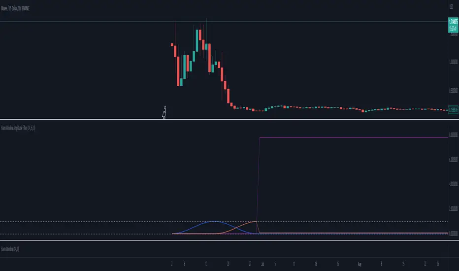
Hann Window Amplitude FilterThis script is designed to implement a multi-signal Hann filter, which is essentially a movable Hann window filter. The purpose of this filter is to allow users to select the periods or frequencies that best align with their trading strategy or market analysis.
The Hann window filter operates by enabling the selection of either lower or higher frequencies. The period of the window is twice the number of signals you wish to filter. As you shift the window by the number of your signals, the signal on one side will have an amplitude of 0, while the other side will have an amplitude of 1.
Continuing to shift the window will result in new values of 0. This feature is particularly useful for further filtering the frequencies or periods that you want to focus on for your trading decisions.
In summary, this script provides a flexible and customizable tool for filtering signals based on their frequency or period, which can be a valuable addition to any trader's technical analysis toolkit.
Statistical Histogram with configurable bins and Data WindowCreates a Histogram for Statistical Analysis of any source.
Input Parameters:
Sample Source: Select your source here, can be any numerical source.
Sample Period: Sample size for Mean and Standard Deviation Calculations.
Enable Cumulative Mode: Will attempt to calculate the bin for every sample in the entire dataset.
Window Period: Used only in Window Mode (Enable Cumulative Mode unchecked), Calculates the bin for the past Window Period sample size.
Bin Label Spacing: Adjust horizontal spacing of Bin Labels below the histogram for easier viewing.
Center Bin: Selects the center Bin, usually set to (0 - Bin Width) < Sample <= 0 standard deviations or (z_score)
Bin Width: Selects the Bin Width in standard deviations.
How you can use it:
View characteristics of dataset such as unimodal/bimodal and skewness to determine preferred statistical analysis.
Additional Reference:
en.wikipedia.org
en.wikipedia.org
Credits:
Thanks goes out to www.tradingview.com , for cleaning up some of the code and www.tradingview.com for the original idea.
Usage Tips:
When adjusting the bin parameters, center bin and bin width, verify that the total sum of the bins (Sum Frequency in the Data Window) is close to the Total Samples. If your Sum Frequency is drastically lower it means you need to adjust your center bin and/or bin width to capture more of the data available.

RSI w/Hann WindowingThis RSI by John Ehlers of "Yet Another" Improved RSI. Taking advantage of the Hann windowing. As seen on PRC and published by John Ehlers, it has a zero mean and appears smoother than the classic RSI. In his own words " I prefer oscillator-type indicators to have a zero mean. We can achieve this simply by multiplying the classic RSI by 2 so it swings from 0 to 2, and then subtract 1 from the product so the indicator swings from -1 to +1." Ehlers goes on to say " Bear in mind 14 may not be the best length to analysis. So, the best length to use for the RSIH indicator is on the order of the dominant cycle period of the data."
This indicator works well with both bullish and bearish divergences. It also works well with oversold and overbought indications. Shown by the Red zone on top (Overbought) and the green zone on the bottom(oversold). Each which have an adjustable buffer zone. You may need to adjust the length of the RSIH to suit your asset. There are also multiply signal line's to choose from. Also take note of when the RSIH crosses up or down on the signal line.
None of this is financial advice.

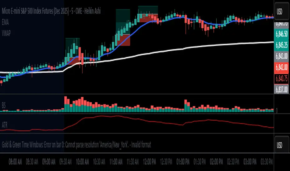
Daily Session Windows background highlight indicatorIn intraday studies of stock indexes and Forex I have this weird habit of highlighting premarket, core session, lunch break and extended session with different backgrounds. If done by hand, this is tedious work that has to be repeated daily.
I think this feature should be built-in in TradingView. But it isn't.
For a few months now, I have been using this tiny indicator that does precisely that job. It saved me literally hours of focus time and mistakes. I have decided to revamp it and release it. I'm sure it can be useful to others.
Features:
Background color highlighting for premarket , core session , lunch hour and extended session of the trading day.
Session timing preset to match US session, but can be customized.
Can be enabled or disabled on a day of the week basis, including week-end.
Timezone is selectable, matches the chart's instrument but can be set independently to track a different timezone.
Not affected by the timezone you decided to assign to the chat's time scale.
Ready for stock indexes, but can be used to highlight Forex sessions too.


Week Window AlgorithmWeek Window Algorithm
The Week Window Algorithm is an advanced intraday trading overlay built for precision session tracking and key level visualization.
🔹 Features:
1. Time Lines
Automatically plots vertical lines 30 minutes ahead of specific London times (07, 08, 09, 13, 14, 15UK), with adjustable height in pips and custom color.
2. Session Boxes
Draws price range boxes for:
Asia (22:00–06:00 UK)
Europe AM (08:00–09:00 UK)
Europe PM (14:00–15:00 UK)
Each box auto-updates during the session and fades after 3 days. Fill color is fully customizable via settings.
3. Yesterday’s High/Low Levels
Captures and plots yesterday’s high and low at 23:00 UK. Lines extend through today and highlight first-time hits.
🛠️ Customization:
Enable/disable sessions individually
Set pip size for early lines
Choose colors for each session box and line style
🕒 Recommended Timeframes:
Optimized for 1–15 minute charts. Works best on intraday setups.

Highlight Trading Window (Simple Hours / Time of Day Filter)As the name says this is a straightforward way to highlight the times of day that you are interested in studying.
Like to trade just a market open, or highlight a full session?
Could also be used negatively to "block out" a window of time each day.
Usage:
Just set your preferred time zone and then your time window (start and end).
Hope you find it useful! 😁

Ehlers Hann Moving Average [CC]The Hann Moving Average is an original script but a slightly modified version of the Hann Window Filter created by John Ehlers. I am using the same length but changed the default data source to use the new Weighted Close that tv added after I requested it awhile ago so thank you tv! The big strength of this moving average/filter is that it creates an extremely smooth filter with the added benefit of very little lag to smooth ratio. The weakness of this moving average/filter is that it does have a decent amount of lag which means it isn't as useful during choppy periods but does work well for sustained uptrends or downtrends. Feel free to experiment and let me know what settings work better for you. I have included strong buy and sell signals in addition to normal ones so strong signals are darker in color and normal signals are lighter in color. Buy when the line turns green and sell when it turns red.
Let me know if there are any other indicators or scripts you would like to see me publish!

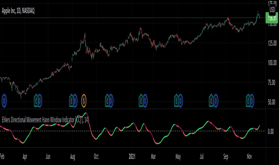
Ehlers Directional Movement Hann Window Indicator [CC]The Directional Movement Hann Window Indicator was created by John Ehlers (Stocks and Commodities Dec 2021 pgs 17-18) and this is his updated version of the classic Directional Movement indicator created by J. Welles Wilder. Ehlers uses the Hann Window Filtering after using an exponential moving average to smooth the classic directional movement indicator. This helps significantly with the lag and lack of smoothing which are both issues with the classic indicator. I have included strong buy and sell signals in addition to the normal ones so strong signals are darker in color and normal signals are lighter in color. Buy when the line turns green and sell when it turns red.
Let me know if there are any other indicators you would like to see me publish!
Dollar Cost Average (Data Window Edition)Hi everyone
Hope you had a nice weekend and you're all excited for the week to come. At least I am (thanks to a few coffee but that still counts !!!)
This indicator is inspired from Dollar-Cost-Average-Cost-Basis
EDUCATIONAL POST
The educational post is coming a bit later this afternoon explaining how to use the indicator so I would advise to follow me so that you'll get updated in real-time :) (shameless self-advertising)
1 - What is Dollar-Cost Averaging (DCA)?
Dollar-Cost Averaging is a strategy that allows an investor to buy the same dollar amount of an investment on regular intervals. The purchases occur regardless of the asset's price.
I hope you're hungry because that one is a biggie and gave me a few headaches. Happy that it's getting out of my way finally and I can offer it
This indicator will analyse for the defined date range, how a dollar cost average (DCA) method would have performed vs investing all the hard earnt money at the beginning
2- What's on the menu today ?
Please check this screenshot to understand what you're supposed to see : CLICK ME I'M A SCREENSHOT (I'll repeat this URL one more time below as I noticed some don't read the information on my description and then will come pinging me saying "sir me no understand your indicator, itz buggy sir"
(yes I finally thought about a way to share screenshots on TradingView, took me 4 weeks, I'm slow to understand things apparently)
My indicator works with all asset classes and with the daily/weekly/monthly timeframes
As always, let's review quickly the different fields so that you'll understand how to use it (and I won't get spammed with questions in DM ^^)
- Use current resolution : if checked will use the resolution of the chart
- Timeframe used for DCA : different timeframe to be used if Use current resolution is unchecked
- Amount invested in your local currency : The amount in Fiat money that will be invested at each period selected above
- Starting Date
- Ending Date
- Select a candle level for the desired timeframe : If you want to use the open or close of the selected period above. Might make a diffence when the timeframe is weekly or monthly
3 - Specifications used
I got the idea from this website dcabtc.com and the result shown by this website and my indicator are very interesting in general and for your own trading
The formula used for the DCA calculation is that one : Investopedia Dollar Cost Average
4 - How to interpret the results
"But sir which results ??"...... those ones : CLICK ME I'M A SCREENSHOT :) (strike #2 with the screenshot)
It will draw all the plots and will give you some nice data to analyze in the Data Window section of TradingView
I'm not completely satisfied with the tool yet but the results are very closed to the dcabtc website mentioned above
If you're trading a very bullish asset class (who said crypto ?), it's very interesting to see what a DCA strategy could bring in term of performance. But DCA is not magic, there is a time component which is the day/week/month you'll start to invest (those who invested in crypto beginning of 2018 in altcoins know what I'm talking about and ..............will hate me for this joke)
5 - What's next ?
As said, the educational post is coming next but not only.
Will probably post a strategy tomorrow using this indicator so that you can compare what's performing best between your trading and a dollar cost average method
I'll publish as a protected source this time a more advanced version of that one including DCA forecasts
6 - Suggested alternative (but I'll you doing it)
If you don't want to have this panel in the bottom with the plots and analyze the results in the data window, you can always create an infopanel like shown here Risk-Reward-InfoPanel/ and display all the data there
Hope you'll like it, like me, love it, love me, tip me :)
____________________________________________________________
Feel free to hit the thumbs up as it shows me that I'm not doing this for nothing and will motivate to deliver more quality content in the future. (Meaning... a few likes only = no indicators = Dave enjoying the beach)
- I'm an offically approved PineEditor/LUA/MT4 approved mentor on codementor. You can request a coaching with me if you want and I'll teach you how to build kick-ass indicators and strategies
Jump on a 1 to 1 coaching with me
- You can also hire for a custom dev of your indicator/strategy/bot/chrome extension/python

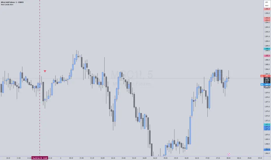
New Candle Alert with Time WindowJust needed a way to specify a time window on a timeframe and get alerts for each new candle
First Window Box + Asia Open HourFirst Window Box + Asia Open Hour is an indicator which marks the High and Low of the Asia Open First hour along with the range marking of First Four Hour and its lenght comparing to the length of last 10 days first four hour range.


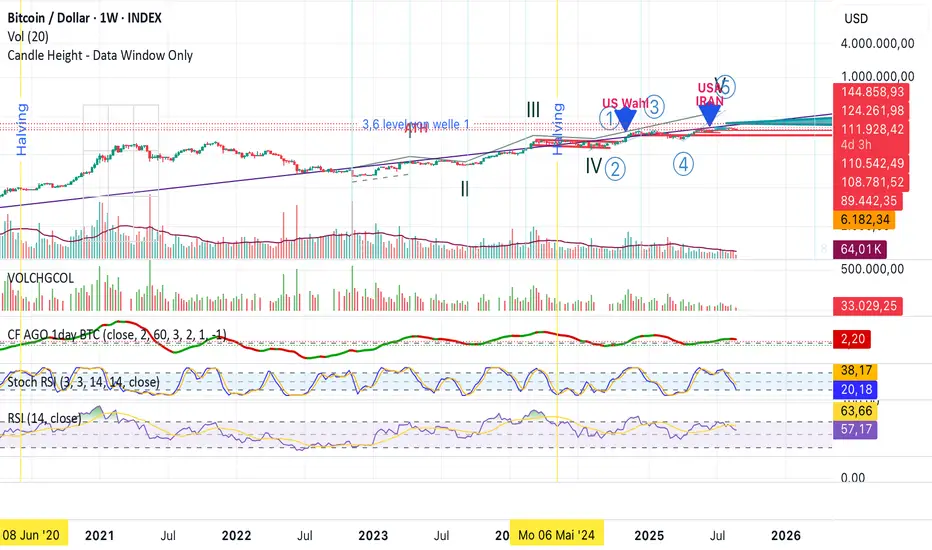
Candle Height - Data Window Onlya simple script showing the height of a candle in the data window when howering about it.
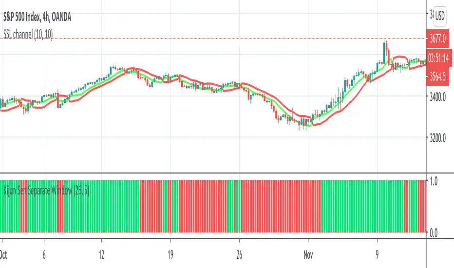
Kijun Sen Separate WindowThis indicator works the same as a regular Kijun Sen but it is on a separate window to allow for other on chart indicators.
I tend to use this as a filter for when to go long/short.
When it is green, I only take longs. When it is red, I only take shorts. Combine with other indicators of your choice.
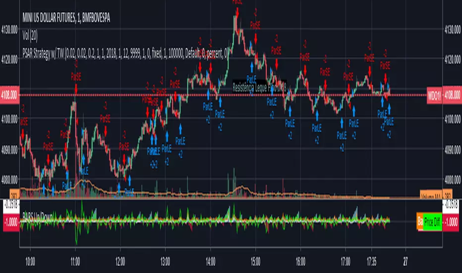
How To Auto Set Date RangeExample how to automatically set the date range window to be backtested from X days or weeks ago to present. Additional options are also included to manually set the date range or to show entire range available.
Normally when you change chart period it changes the number of days being backtested, which means as you increase the chart period (for example from 5min to 15min), you also increase the number of days traded. So you can not compare apples to apples for which period would yield best performance for your strategy.
By incorporating this code with your own strategy's logic (replacing buy and sell), it will allow you to compare results of different period backtests over the same duration of time.
Date Range: ALL uses entire history.
Date Range: DAYS uses number you set in # Days or Weeks
Date Range: WEEKS uses number you set in # Days or Weeks
Date Range: MANUAL uses manual dates you set in From and To fields
Much gratitude to @pinechrix for suggesting this improvement to me, and to @Gesundheit for pointing me in the right direction on the original example I published previously. Thank you both!
NOTICE: This is an example script and not meant to be used as an actual strategy. By using this script or any portion thereof, you acknowledge that you have read and understood that this is for research purposes only and I am not responsible for any financial losses you may incur by using this script!

How To Set Backtest Date RangeExample how to select and set date range window to be backtested. Normally when you change chart period it changes the number of days being backtested which means as you increas the chart period (for example from 5min to 15min) you also increase the number of days traded, so you can not compare apples to apples for which period would yield best returns for your strategy. Now you can. Incorporate this code replacing buy and sell with your strategy, then simply input the From and To dates in Format -> Inputs, and then change the chart period to view updated results.
NOTE: There is a limit in backtesting to 2000 orders, so please be aware of this when setting your date ranges. If you set your range too high, you may be exceeding this limit on some periods and not on others, so this would yield incorrect comparison of returns per period. If you see in your backtesting results that you are nearing this limit for one of your periods you are testing, then reduce the date range to a smaller number of days.
Enjoy!
(Thanks to @Gesundheit "Adeel" for pointing me in the right direction on this!)