Gamma & Max Pain HelperGamma & Max Pain Helper
Plots Call Wall, Put Wall, and Max Pain levels directly on your chart so you can see where options positioning might influence price.
Features:
Manually enter Call Wall, Put Wall, and Max Pain strike prices.
Lines auto-update each bar — no redrawing needed.
Labels display name + strike price.
Option to only show lines near current price (within a % you choose).
Color-coded:
Red = Call Wall (potential resistance)
Green = Put Wall (potential support)
Blue = Max Pain (price magnet into expiry)
Adjustable line width & extension.
Use Case:
Perfect for traders combining options open interest/gamma analysis with price action, pivots, VWAP, and other intraday levels. Quickly spot overlaps between option walls and technical barriers for high-probability reaction zones.
在腳本中搜尋"富国恒生港股通高股息低波动ETF发起式联接A+高股息低波动优势"

Source-indicatorsSource Indicators – A premium TradingView tool combining automated support/resistance levels, dynamic trendlines, and breakout alerts.
Perfect for spotting key market zones and trend shifts in real-time.
Quant Signals: Market Sentiment Monitor HUDWavelets & Scale Spectrum
This indicator is ideal for traders who adapt their strategy to market conditions — such as swing traders, intraday traders, and system developers.
Trend-followers can use it to confirm trending conditions before entering.
Mean-reversion traders can spot choppy markets where reversals are more likely.
Risk managers can monitor volatility shifts and regime changes to adjust position size or pause trading.
It works best as a market context filter — telling you the “weather” before you decide on the trade.
Wavelets are like tiny “measuring rulers” for price changes. Instead of looking at the whole chart at once, a wavelet looks at differences in price over a specific time scale — for example, 2 bars, 4 bars, 8 bars, and so on.
The scale spectrum is what you get when you measure volatility at several of these scales and then plot them against scale size.
If the spectrum forms a straight line on a log–log chart, it means price changes follow a consistent pattern across time scales (a power-law relationship).
The slope of that line gives the Hurst exponent (H) — telling you whether moves tend to persist (trend) or reverse (mean-revert).
The height of the line gives you the volatility (σ) — the average size of moves.
This approach works like a microscope, revealing whether the market’s behaviour is consistent across short-term and long-term horizons, and when that behaviour changes.
This tool applies a wavelet-based scale-spectrum analysis to price data to estimate three key market state measures inside a rolling window:
Hurst exponent (H) — measures persistence in price moves:
H > ~0.55 → market is trending (moves tend to continue).
H < ~0.45 → market is choppy/mean-reverting (moves tend to reverse).
Values near 0.5 indicate a neutral, random-walk-like regime.
Volatility (σ) — the average size of price swings at your chart’s timeframe, optionally annualized. Rising volatility means larger price moves, falling volatility means smaller moves.
Fit residual — how well the observed multi-scale volatility fits a clean power-law line. Low residual = stable behaviour; high residual = structural change (possible regime shift).
Whaley Thrust — ADT / UDT / SPT (2010) + EDT (EMA) + Info BoxDescription
Implements Wayne Whaley’s 2010 Dow Award breadth-thrust framework on daily data, with a practical extension:
• ADT (Advances Thrust) — 5-day ratio of advances to (adv+dec). Triggers: > 73.66% (thrust), < 19.05% (capitulation).
• UDT (Up-Volume Thrust) — 5-day ratio of up-volume to (up+down). Triggers: > 77.88%, < 16.41%. Defaults to USI:UVOL / USI:DVOL (edit if your feed differs).
• SPT (Price Thrust) — 5-day % change of a benchmark (default SPY, toggle to use chart symbol). Triggers: > +10.05%, < −13.85%.
• EDT (EMA extension) — Declines-share thrust derived from WBT logic (not in Whaley’s paper): EMA/SMA of Declines / (Adv+Decl). Triggers: > 0.8095 (declines thrust), < 0.2634 (declines abating).
• All-Clear — Prints when ADT+ and UDT+ occur within N days (default 10); marks the second event and shades brighter green.
Visuals & Controls
• Shape markers for each event; toggle text labels on/off.
• Optional background shading (green for thrusts, red for capitulations; brighter green for All-Clear).
• Compact info box showing live ADT / UDT / SPT (white by default; turns green/red at thresholds).
• Min-spacing filter to prevent duplicate prints.
Tips
• Use on Daily charts (paper uses 5 trading days). Weekly views can miss mid-week crosses.
• If UDT shows 100%, verify your Down Volume symbol; the script requires both UVOL and DVOL to be > 0.
• Best use: treat capitulations (−) as setup context; act on thrusts (+)—especially when ADT+ & UDT+ cluster (All-Clear).
Credit
Core method from Wayne Whaley (2010), Planes, Trains and Automobiles (Dow Award). EDT is an added, complementary interpretation using WBT-style smoothing.

Quant Signals: Entropy w/ ForecastThis is the first of many quantitative signals I plan to create for TV users.
Most technical analysis (TA) tools—like moving averages, oscillators, or chart patterns—are heuristic: they’re based on visually identifiable shapes, threshold crossovers, or empirically chosen rules. These methods rarely quantify the information content or structural complexity of market data. By quantifying market predictability before making a forecast, this method filters out noise and focuses your trading only during statistically favorable conditions—something traditional TA cannot objectively measure.
This MEPP-based approach is quantitative and model-free:
It comes from information theory and measures Shannon entropy rate to assess how predictable the market is at any moment.
Instead of interpreting price formations, it uses a data-compression algorithm (Lempel–Ziv) to capture hidden structure in the sequence of returns.
Forecasts are generated using a principle from statistical physics (Maximum Entropy Production), not historical chart patterns.
In short, this method measures the market's predictability BEFORE deciding a directional forecast is worth trusting. This tool is to inform TA traders on the market's current regime, whether it is smooth and predictable or it is volatile and turbulent.
Technical Introduction:
In information theory, Shannon entropy measures the uncertainty (or information content) in a sequence of data. For markets, the entropy rate captures how much new information price returns generate over time:
Low entropy rate → price changes are more structured and predictable.
High entropy rate → price changes are more random and unpredictable.
By discretizing recent returns into quartile-based states, this indicator:
Calculates the normalized entropy rate as a regime filter.
Uses MEPP to forecast the next state that maximizes entropy production.
Displays both the regime status (predictable vs chaotic) and the forecast bias (bullish/bearish) in a dashboard.
Measurements & How to Use Them
TLDR: HIGH ENTROPY -> information generation/market shift -> Don't trust forecast/strategy
1. H (bits/sym)
Shannon entropy rate of the last μ discrete returns, in bits per symbol (0–2).
Lower → more predictable; higher → more random.
Use as a raw measure of market structure.
2. H_max (log₂Ω)
Theoretical maximum entropy for Ω states. Here Ω = 4 → H_max = 2.0 bits.
Reference value for normalization.
3. Entropy (norm)
H / H_max, scaled between 0 and 1.
< 0.5–0.6 → predictable regime; > 0.6 → chaotic regime.
Main regime filter — forecasts are more reliable when below your threshold.
4. Regime
Label based on Entropy (norm) vs your entThresh.
LOW (predictable) = higher odds forecast will be correct.
HIGH (chaotic) = forecasts less reliable.
5. Next State (MEPP Forecast)
Discrete return state (1–4) predicted to occur next, chosen to maximize entropy production:
Large Down (strong bearish)
Small Down (mild bearish)
Small Up (mild bullish)
Large Up (strong bullish)
Use as your bias direction.
6. Bias
Simplified label from the Next State:
States 1–2 = Bearish bias (red)
States 3–4 = Bullish bias (green)
Align strategy direction with bias only in LOW regime.
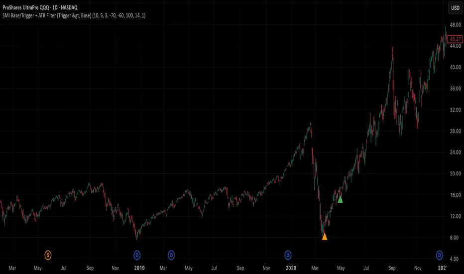
SMI Base-Trigger Bullish Re-acceleration (Higher High)Description
What it does
This indicator highlights a two-step bullish pattern using Stochastic Momentum Index (SMI) plus an ATR distance filter:
1. Base (orange) – Marks a momentum “reset.” A base prints when SMI %K crosses up through %D while %K is below the Base level (default -70). The base stores the base price and starts a waiting window.
2. Trigger (green) – Confirms momentum and price strength. A trigger prints only if, before the timeout window ends:
• SMI %K crosses up through %D again,
• %K is above the Trigger level (default -60),
• Close > Base Price, and
• Price has advanced at least Min ATR multiple (default 1.0× the 14-period ATR) above the base price.
A dashed green line connects the base to the trigger.
Why it’s useful
It seeks a bullish divergence / reacceleration: momentum recovers from deeply negative territory, then price reclaims and exceeds the base by a volatility-aware margin. This helps filter out weak “oversold bounces.”
Signals
• Base ▲ (orange): Potential setup begins.
• Trigger ▲ (green): Confirmation—momentum and price agree.
Inputs (key ones)
• %K Length / EMA Smoothing / %D Length: SMI construction.
• Base when %K < (default -70): depth required for a valid reset.
• Trigger when %K > (default -60): strength required on confirmation.
• Base timeout (days) (default 100): maximum look-ahead window.
• ATR Length (default 14) and Min ATR multiple (default 1.0): price must exceed the base by this ATR-scaled distance.
How traders use it (example rules)
• Entry: On the Trigger.
• Risk: A common approach is a stop somewhere between the base price and a multiple of ATR below trigger; or use your system’s volatility stop.
• Exits: Your choice—trend MA cross, fixed R multiple, or structure-based levels.
Notes & tips
• Works best on liquid symbols and mid-to-higher timeframes (reduce noise).
• Increase Min ATR multiple to demand stronger price confirmation; tighten or widen Base/Trigger levels to fit your market.
• This script plots signals only; convert to a strategy to backtest entries/exits.
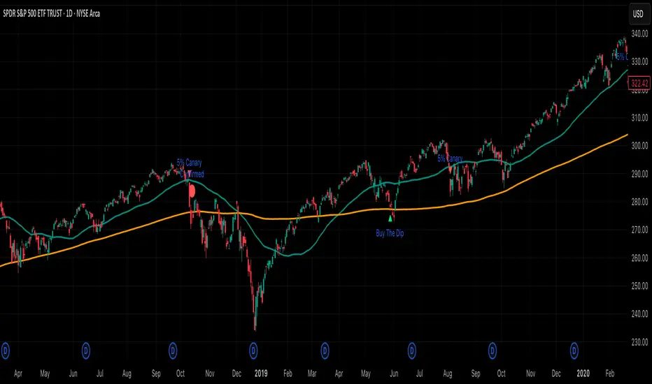
5% Canary (per Thrasher) Implements Thrasher’s framework using closing prices and simple, non-optimized thresholds. The study watches for the first 5% decline from the latest 52-week closing high and classifies it:
• 5% Canary: drop occurs in ≤ 15 trading days.
• Confirmed 5% Canary: within 42 trading days of a Canary, there are two consecutive closes below the 200-DMA.
• Buy-the-Dip: the first 5% decline takes > 15 days and 50-DMA > 200-DMA (uptrend).
Includes optional 50/200-DMA plots, clutter-reduction, and alert conditions. This is a signal framework, not a standalone system—pair with your own risk management.
Entropy (Fiedor/Kontoyiannis) - Part 2 of Fiedor's TheoryThis indicator estimates the Shannon entropy of a price series using a Markov chain model of binary returns, following the approach of Fiedor (2014) and Kontoyiannis (1997).
% of Max shows current entropy as a percentage of its theoretical maximum (1 bit for binary up/down moves).
Percentile ranks the current entropy against historical values in the chosen lookback window.
High entropy suggests price movement is less predictable by frequentist models; low entropy implies more structure and predictability.
Use this as an informational oscillator, not a trading signal.
This is a visualization of Part 1 of Fiedor's Theory. The same entropy logic is already embedded in Part 1 however the second pane is a nice reminder of why it works.

EMA band 12/60/150/200EMA band consisting of 12/60/150/200
Specifically for Indian stock market, can be used for other trading scripts after testing.
Best use case : on Daily TF.
Bull run entry criteria, Not bear market or Bottom catching.

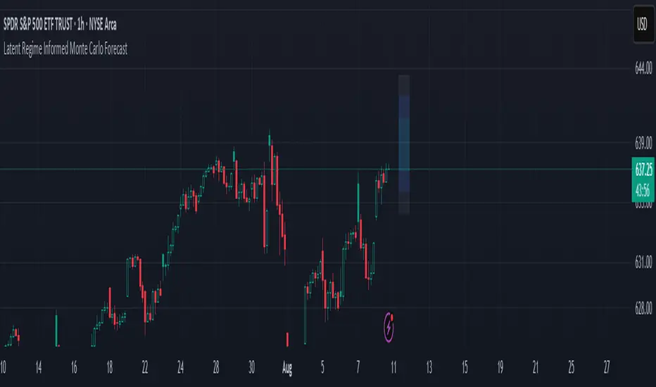
Latent Regime Informed Monte Carlo ForecastThis script uses a Monte Carlo simulation to forecast where price might be a set number of bars into the future (default 6 bars ahead). It generates hundreds of possible future price paths based on an average move (drift) and random shocks (volatility). The result is a distribution of outcomes, displayed as probability zones: the median (most likely), inner bands (50% confidence), and wider bands (80% and 95% confidence). Due to the randomness assumption in Monte Carlo simulations, the paths are not very important so to minimize cluttering on the graphs we only plot bands. These zones help you visualize uncertainty, set stops and targets based on probabilities, and spot when market behavior changes.
The accuracy of any Monte Carlo forecast depends heavily on how well you estimate trend and volatility. By default and no prior information the Monte Carlo simulation gives you a parabolic forecast that assumes absolute randomness. This is where the Kalman filter comes in. The filter (derived from control theory) aims to detect latent (unobservable) traits about the system by continuously updating its transition probabilities to better understand how the latent traits affect the observable measurement (price). With each new observable state we get better and better transition probabilities and enhances our understanding about the latent and unobservable market characteristics like trend and volatility. Both crucial measurements for short term market sentiment.
Extracting these measurements for market sentiment informs us how to better parametrize the Monte Carlo simulation for a better forecast. Each bar, the KF updates its estimates based on how close its last prediction was to reality. In calm periods, it holds estimates steady; in volatile periods, it adapts quickly. This gives you real-time, low-lag measurements of both trend and volatility.
By feeding these adaptive estimates into the Monte Carlo simulation, the forecast becomes much more responsive to current market conditions. In trends, the predicted paths tilt toward the direction of movement; in choppy markets, they spread wider but stay centered; when volatility spikes, the probability zones expand immediately. The result is a dynamic forecast tool that adjusts on every bar, giving you a clearer, probability-based picture of where the market could go next.
This is my very first script and I would love feedback/ideas for different topics.
My background is in economics/mathematics and interests lie in time series analysis/exploring financial features for DS
Volume Profile (Simple)Simple Volume Profile (Simple)
Master the Market's Structure with a Clear View of Volume
by mercaderoaurum
The Simple Volume Profile (Simple) indicator removes the guesswork by showing you exactly where the most significant trading activity has occurred. By visualizing the Point of Control (POC) and Value Area (VA) for today and yesterday, you can instantly identify the price levels that matter most, giving you a critical edge in your intraday trading.
This tool is specifically optimized for day trading SPY on a 1-minute chart, but it's fully customizable for any symbol or timeframe.
Key Features
Multi-Day Analysis: Automatically plots the volume profiles for the current and previous trading sessions, allowing you to see how today's market is reacting to yesterday's key levels.
Automatic Key Level Plotting: Instantly see the most important levels from each session:
Point of Control (POC): The single price level with the highest traded volume, acting as a powerful magnet for price.
Value Area High (VAH): The upper boundary of the area where 50% of the volume was traded. It often acts as resistance.
Value Area Low (VAL): The lower boundary of the 50% value area, often acting as support.
Extended Levels: The POC, VAH, and VAL from previous sessions are automatically extended into the current day, providing a clear map of potential support and resistance zones.
Customizable Sessions: While optimized for the US stock market, you can define any session time and time zone, making it a versatile tool for forex, crypto, and futures traders.
Core Trading Strategies
The Simple Volume Profile helps you understand market context. Instead of trading blind, you can now make decisions based on where the market has shown the most interest.
1. Identifying Support and Resistance
This is the most direct way to use the indicator. The extended lines from the previous day are your roadmap for the current session.
Previous Day's POC (pPOC): This is the most significant level. Watch for price to react strongly here. It can act as powerful support if approached from above or strong resistance if approached from below.
Previous Day's VAH (pVAH): Expect this level to act as initial resistance. A clean break above pVAH can signal a strong bullish trend.
Previous Day's VAL (pVAL): Expect this level to act as initial support. A firm break below pVAL can indicate a strong bearish trend.
Example Strategy: If SPY opens and rallies up to the previous day's VAH and stalls, this is a high-probability area to look for a short entry, with a stop loss just above the level.
2. The "Open-Drive" Rejection
How the market opens in relation to the previous day's value area is a powerful tell.
Open Above Yesterday's Value Area: If the market opens above the pVAH, it signals strength. The first pullback to test the pVAH is often a key long entry point. The level is expected to flip from resistance to support.
Open Below Yesterday's Value Area: If the market opens below the pVAL, it signals weakness. The first rally to test the pVAL is a potential short entry, as the level is likely to act as new resistance.
3. Fading the Extremes
When price pushes far outside the previous day's value area, it can become overextended.
Reversal at Highs: If price rallies significantly above the pVAH and then starts to lose momentum (e.g., forming bearish divergence on RSI or a topping pattern), it could be an opportunity to short the market, targeting a move back toward the pVAH or pPOC.
Reversal at Lows: Conversely, if price drops far below the pVAL and shows signs of bottoming, it can be a good opportunity to look for a long entry, targeting a reversion back to the value area.
Recommended Settings (SPY Intraday)
These settings are the default and are optimized for scalping or day trading SPY on a 1-minute chart.
Value Area (%): 50%. This creates a tighter, more sensitive value area, perfect for identifying the most critical intraday zones.
Number of Rows: 1000. This high resolution is essential for a low-volatility instrument like SPY, ensuring that the profile is detailed and the levels are precise.
Session Time: 0400-1800 in America/New_York. This captures the full pre-market and core session, which is crucial for understanding the day's complete volume story.
Ready to trade with an edge? Add the Simple Volume Profile (Multi-Day) to your chart now and see the market in a new light!
Bullish Divergence SMI Base & Trigger with ATR FilterDescription:
A bullish divergence indicator combining the Stochastic Momentum Index (SMI) and Average True Range (ATR) to pinpoint high-probability entries:
1. Base Arrow (Orange ▲):
• Marks every SMI %K / %D bullish crossover where %K < –70 (deep oversold)—the first half of the divergence setup.
• Each new qualifying crossover replaces the previous base, continuously “arming” the divergence signal.
• Configurable SMI lookbacks, oversold threshold, and a base timeout (default 100 days) to clear stale bases.
2. Trigger Arrow (Green ▲):
• Completes the bullish divergence: fires on the next SMI bullish crossover where %K > –60 and price has dropped below the base arrow’s close by at least N × ATR (default 1 × 14-day ATR).
• A dashed green line links the base and trigger to visually confirm the divergence.
• Resets after triggering, ready for a new divergence cycle.
Inputs:
• SMI %K Length, EMA Smoothing, %D Length
• Oversold Base Level (–70), Trigger Level (–60)
• ATR Length (14), ATR Multiplier (1.0)
• Base Timeout (100 days)
Ideal for any market, this study highlights genuine bullish divergences—oversold momentum crossovers that coincide with significant price reactions—before entering long trades.

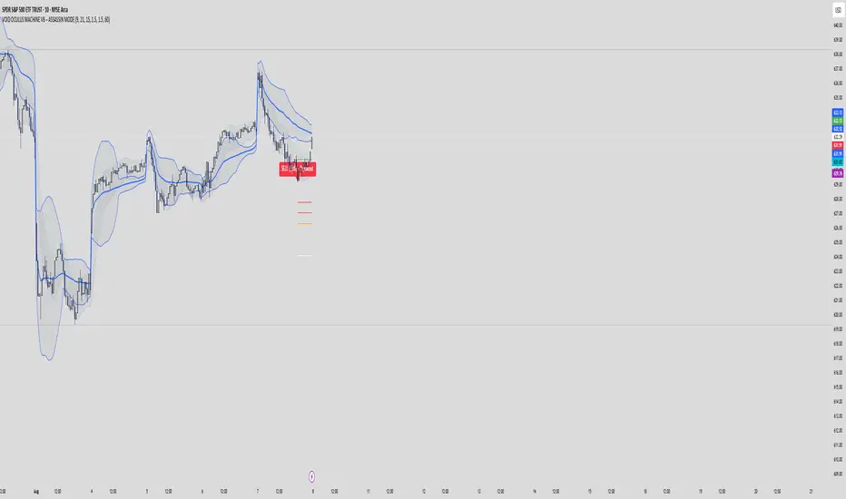
VOID OCULUS MACHINE V8 – ASSASSIN MODEVOID OCULUS MACHINE V8 – ASSASSIN MODE
Version 8.0 | Pine Script v6
Purpose & Originality
VOID OCULUS MACHINE V8 – ASSASSIN MODE brings together four advanced trading filters—EMA crossovers, TRIX momentum, VWAP band positioning, and a proprietary “Predictive Cloud”—into a single, high-precision entry system. Rather than relying on any one signal, it calculates a confidence score combining trend, momentum, volume, and volatility cues, then triggers only the highest-probability setups once a user-defined threshold is met. This multi-layer architecture offers traders laser-focused entries (“Assassin Mode”) with built-in risk (stop) and reward (targets) visualization.
How It Works & Component Rationale
EMA Trend Alignment
Fast EMA (9) vs. Slow EMA (21): Captures short-term versus medium-term trend. A bullish bias requires EMA9 > EMA21, bearish bias EMA9 < EMA21.
TRIX Momentum Filter
A triple-smoothed EMA oscillator over 15 bars, expressed as a percentage change. Positive TRIX confirms upward momentum; negative TRIX confirms downward momentum.
Gaussian Noise Reduction
Dual 5-period EMA smoothing of price removes short-term noise, creating a “cloud base.” Entries only fire when price interacts favorably with this smoothed baseline.
VWAP Band Confirmation (Optional)
Calculates session VWAP ± one standard deviation over 20 bars, plotting upper/lower bands. Traders can require price to sit above/below VWAP mid for trend confirmation.
Predictive Cloud Overlay
A dynamic band (Gaussian ± ATR) forecasts a near-term “value zone.” Pullback and reversal entries can occur as price re-enters or breaks out of this cloud.
Confidence Scoring
Starts at 0 and adds:
+30 for EMA trend alignment (bull or bear)
+20 for volume spike (>20-bar SMA)
+20 for non-zero TRIX slope
+20 for ATR expansion (volatility ramping)
+10 if price is above or below VWAP mid (if VWAP filter is enabled)
Only fires signals when confidence ≥ 60% (configurable), ensuring multi-factor confluence.
Entry Type Differentiation
Breakout: Price pierces prior 10-bar high/low on volume and ATR expansion.
Pullback: Trend bias plus a crossover of price with EMA9.
Reversal: Price crosses back into the Predictive Cloud from outside, confirmed by VWAP cross.
Automated Trade Visualization
On each signal, clears previous objects, plots a “BUY (xx%) – ” or “SELL (xx%) – ” label, four tiered ATR-based targets (1×, 1.5×, 2×, 3.5×), and a stop-loss (ATR × 1.5).
Inputs & Customization
Input Description Default
Fast EMA Length for short-term trend EMA 9
Slow EMA Length for medium-term trend EMA 21
TRIX Length Period for triple-smoothed momentum oscillator 15
Stop Multiplier ATR multiple for stop-loss distance 1.5
Target Multiplier ATR multiple for first profit target 1.5
Enable VWAP Filter Require price alignment above/below VWAP mid On
Minimum Confidence Confidence % threshold to trigger a signal 60
Show Predictive Cloud Toggle the Gaussian ± ATR cloud on/off On
How to Use
Apply to Chart: Suitable on 5 m–1 h timeframes for swing entries.
Adjust Confidence & Filters: Raise the Minimum Confidence to tighten setups; disable VWAP filter for pure price/momentum plays.
Read Signals:
“BUY (75%) – Breakout” label means 75% confluence across filters, triggered by a breakout entry type.
Four colored horizontal lines mark TP1–TP4; a red line marks your stop.
Manage the Trade:
Use the plotted stop-loss line; scale out at targets or trail behind the Predictive Cloud.
Unique Value
VOID OCULUS MACHINE V8 stands out by quantifying multi-dimensional market context into a single confidence score and providing automated trade object plotting—no more manual target calculations or cluttered charts. Its “Assassin Mode” ensures only the most compelling setups trigger, saving traders time and reducing noise.
Disclaimer
This indicator is for educational purposes. Past performance does not guarantee future results. Always backtest across symbols/timeframes, combine with personal discretion, and apply strict risk management before trading live.
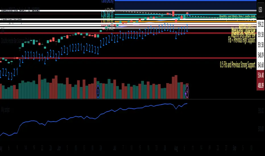
Double Inside Bar Scanner [Daily]Double Inside Bar Scanner . Captures Double Inside based on last 2 daily Bars
Multi-Signal Entry V1Multi‑Signal Entry v1 – (clean, versioned for tracking changes)
SQQQ Entry Scanner – (specific to your use case)
TQQQ/SQQQ Buy Alert – (clear that it’s for both sides if you add short logic later)
VWAP RSI ATR Vol Spike – (great if you want a technical name showing what’s used)
Fast Entry Signal Bot – (if you want a simple, trading-friendly name)

Dynamic 5DMA/EMA with Color for Multiple Products🔹 Dynamic 5DMA/EMA with Slope-Based Coloring (All Timeframes)
This indicator plots a dynamic 5-period moving average that adapts intelligently to your chart's timeframe and product type — giving you a clean, slope-sensitive visual edge across intraday, daily, and weekly views.
✅ Key Features:
📈 Dynamic MA Length Scaling:
On intraday timeframes, the MA adjusts for your selected market session (RTH, ETH, VIX, or Futures), calculating a true 5-day average based on actual session length — not just a flat bar count.
🔄 Automatic Timeframe Detection:
Daily Chart: Uses standard 5DMA or 5EMA.
Weekly Chart: Applies a true 5-week MA.
Intraday Charts: Converts 5 days into bar-length equivalent dynamically.
🎨 Color-Coded Slope Logic:
Green = Rising MA (bullish slope)
Red = Falling MA (bearish slope)
Neutral slope = previous color held for visual continuity
No more guessing — direction is instantly clear.
⚠️ Built-In Slope Flip Alerts:
Set alerts when the slope of the MA turns up or down. Ideal for timing pullback entries or exits across any product.
⚙️ Session Settings for Proper Scaling:
Choose your product's market structure to ensure accurate 5-day conversion on intraday charts:
Stocks - RTH: 390 mins/day
Stocks - ETH: 780 mins/day
VIX: 855 mins/day
Futures: 1440 mins/day
This ensures the MA reflects 5 full trading days, regardless of session irregularities or bar interval.
📌 Why Use This Indicator?
Most MAs misrepresent trend direction on intraday charts because they assume static daily bar counts. This tool corrects that, then adds slope-based coloring to give you a fast, visual read on short-term momentum. Whether you’re swing trading SPY, scalping VIX, or position trading futures, this indicator keeps your view aligned with how institutions see moving averages across timeframes.
🔧 Best For:
VIX & volatility traders
Short-term SPY/SPX traders
Swing traders who value clean setups
Anyone wanting a true 5-day trend anchor on any chart
thors_forex_factory_utilityLibrary "forex_factory_utility"
Supporting Utility Library for the Live Economic Calendar by toodegrees Indicator; responsible for data handling, and plotting news event data.
isLeapYear()
Finds if it's currently a leap year or not.
Returns: Returns True if the current year is a leap year.
daysMonth(M)
Provides the days in a given month of the year, adjusted during leap years.
Parameters:
M (int) : Month in numerical integer format (i.e. Jan=1).
Returns: Days in the provided month.
MMM(M)
Converts a month from a numerical integer format to a MMM format (i.e. 'Jan').
Parameters:
M (int) : Month in numerical integer format (i.e. Jan=1).
Returns: Month in MMM format (i.e. 'Jan').
dow(D)
Converts a numbered day of the week string in format to 'DDD' format (i.e. "1" = Sun).
Parameters:
D (string) : Numbered day of the week from 1 to 7, starting on Sunday.
Returns: Returns the day of the week in 'DDD' format (i.e. "Fri").
size(S, N)
Converts a size string into the corresponding Pine Script v5 format, or N times smaller/bigger.
Parameters:
S (string) : Size string: "Tiny", "Small", "Normal", "Large", or "Huge".
N (int) : Size variation, can be positive (larger than S), or negative (smaller than S).
Returns: Size string in Pine Script v5 format.
lineStyle(S)
Converts a line style string into the corresponding Pine Script v5 format.
Parameters:
S (string) : Line style string: "Dashed", "Dotted" or "Solid".
Returns: Line style string in Pine Script v5 format.
lineTrnsp(S)
Converts a transparency style string into the corresponding integer value.
Parameters:
S (string) : Line style string: "Light", "Medium" or "Heavy".
Returns: Transparency integer.
boxLoc(X, Y)
Converts position strings of X and Y into a table position in Pine Script v5 format.
Parameters:
X (string) : X-axis string: "Left", "Center", or "Right".
Y (string) : Y-axis string: "Top", "Middle", or "Bottom".
Returns: Table location string in Pine Script v5 format.
method bubbleSort_NewsTOD(N)
Performs bubble sort on a Forex Factory News array of all news from the same date, ordering them in ascending order based on the time of the day.
Namespace types: array
Parameters:
N (array) : Forex Factory News array.
Returns: void
bubbleSort_News(N)
Performs bubble sort on a Forex Factory News array, ordering them in ascending order based on the time of the day, and date.
Parameters:
N (array) : Forex Factory News array.
Returns: Sorted Forex Factory News array.
weekNews(N, C, I)
Creates a Forex Factory News array containing the current week's Forex Factory News.
Parameters:
N (array) : Forex Factory News array containing this week's unfiltered Forex Factory News.
C (array) : Currency filter array (string array).
I (array) : Impact filter array (color array).
Returns: Forex Factory News array containing the current week's Forex Factory News.
todayNews(W, D, M)
Creates a Forex Factory News array containing the current day's Forex Factory News.
Parameters:
W (array) : Forex Factory News array containing this week's Forex Factory News.
D (array) : Forex Factory News array for the current day's Forex Factory News.
M (bool) : Boolean that marks whether the current chart has a Day candle-switch at Midnight New York Time.
Returns: Forex Factory News array containing the current day's Forex Factory News.
adjustTimezone(N, TZH, TZM)
Transposes the Time of the Day, and Date, in the Forex Factory News Table to a custom Timezone.
Parameters:
N (array) : Forex Factory News array.
TZH (int) : Custom Timezone hour.
TZM (int) : Custom Timezone minute.
Returns: Reformatted Forex Factory News array.
NewsAMPM_TOD(N)
Reformats the Time of the Day in the Forex Factory News Table to AM/PM format.
Parameters:
N (array) : Forex Factory News array.
Returns: Reformatted Forex Factory News array.
impFilter(X, L, M, H)
Creates a filter array from the User's desired Forex Facory News to be shown based on Impact.
Parameters:
X (bool) : Boolean - if True Holidays listed on Forex Factory will be shown.
L (bool) : Boolean - if True Low Impact listed on Forex Factory News will be shown.
M (bool) : Boolean - if True Medium Impact listed on Forex Factory News will be shown.
H (bool) : Boolean - if True High Impact listed on Forex Factory News will be shown.
Returns: Color array with the colors corresponding to the Forex Factory News to be shown.
curFilter(A, C1, C2, C3, C4, C5, C6, C7, C8, C9)
Creates a filter array from the User's desired Forex Facory News to be shown based on Currency.
Parameters:
A (bool) : Boolean - if True News related to the current Chart's symbol listed on Forex Factory will be shown.
C1 (bool) : Boolean - if True News related to the Australian Dollar listed on Forex Factory will be shown.
C2 (bool) : Boolean - if True News related to the Canadian Dollar listed on Forex Factory will be shown.
C3 (bool) : Boolean - if True News related to the Swiss Franc listed on Forex Factory will be shown.
C4 (bool) : Boolean - if True News related to the Chinese Yuan listed on Forex Factory will be shown.
C5 (bool) : Boolean - if True News related to the Euro listed on Forex Factory will be shown.
C6 (bool) : Boolean - if True News related to the British Pound listed on Forex Factory will be shown.
C7 (bool) : Boolean - if True News related to the Japanese Yen listed on Forex Factory will be shown.
C8 (bool) : Boolean - if True News related to the New Zealand Dollar listed on Forex Factory will be shown.
C9 (bool) : Boolean - if True News related to the US Dollar listed on Forex Factory will be shown.
Returns: String array with the currencies corresponding to the Forex Factory News to be shown.
FF_OnChartLine(N, T, S)
Plots vertical lines where a Forex Factory News event will occur, or has already occurred.
Parameters:
N (array) : News-type array containing all the Forex Factory News.
T (int) : Transparency integer value (0-100) for the lines.
S (string) : Line style in Pine Script v5 format.
Returns: void
method updateStringMatrix(M, P, V)
Updates a string Matrix containing the tooltips for Forex Factory News Event information for a given candle.
Namespace types: matrix
Parameters:
M (matrix) : String matrix.
P (int) : Position (row) of the Matrix to update based on the impact.
V (string) : information to push to the Matrix.
Returns: void
FF_OnChartLabel(N, Y, S, O)
Plots labels where a Forex Factory News has already occurred based on its/their impact.
Parameters:
N (array) : News-type array containing all the Forex Factory News.
Y (string) : String that gives direction on where to plot the label (options= "Above", "Below", "Auto").
S (string) : Label size in Pine Script v5 format.
O (bool) : Show outline of labels?
Returns: void
historical(T, D, W, X)
Deletes Forex Factory News drawings which are ourside a specific Time window.
Parameters:
T (int) : Number of days input used for Forex Factory News drawings' history.
D (bool) : Boolean that when true will only display Forex Factory News drawings of the current day.
W (bool) : Boolean that when true will only display Forex Factory News drawings of the current week.
X (string) : String that gives direction on what lines to plot based on Time (options= "Future", "Both").
Returns: void
newTable(P, B)
Creates a new Table object with parameters tailored to the Forex Factory News Table.
Parameters:
P (string) : Position string for the Table, in Pine Script v5 format.
B (color) : Border and frame color for the News Table.
Returns: Empty Forex Factory News Table.
resetTable(P, S, headTextC, headBgC, B)
Resets a Table object with parameters and headers tailored to the Forex Factory News Table.
Parameters:
P (string) : Position string for the Table, in Pine Script v5 format.
S (string) : Size string for the Table's text, in Pine Script v5 format.
headTextC (color)
headBgC (color)
B (color) : Border and frame color for the News Table.
Returns: Empty Forex Factory News Table.
logNews(N, TBL, R, S, rowTextC, rowBgC)
Adds an event to the Forex Factory News Table.
Parameters:
N (News) : News-type object.
TBL (table) : Forex Factory News Table object to add the News to.
R (int) : Row to add the event to in the Forex Factory News Table.
S (string) : Size string for the event's text, in Pine Script v5 format.
rowTextC (color)
rowBgC (color)
Returns: void
FF_Table(N, P, S, headTextC, headBgC, rowTextC, rowBgC, B)
Creates the Forex Factory News Table.
Parameters:
N (array) : News-type array containing all the Forex Factory News.
P (string) : Position string for the Table, in Pine Script v5 format.
S (string) : Size string for the Table's text, in Pine Script v5 format.
headTextC (color)
headBgC (color)
rowTextC (color)
rowBgC (color)
B (color) : Border and frame color for the News Table.
Returns: Forex Factory News Table.
timeline(N, T, F, TZH, TZM, D)
Shades Forex Factory News events in the Forex Factory News Table after they occur.
Parameters:
N (array) : News-type array containing all the Forex Factory News.
T (table) : Forex Facory News table object.
F (color) : Color used as shading once the Forex Factory News has occurred.
TZH (int) : Custom Timezone hour, if any.
TZM (int) : Custom Timezone minute, if any.
D (bool) : Daily Forex Factory News flag.
Returns: Forex Factory News Table.
News
Custom News type which contains informatino about a Forex Factory News Event.
Fields:
dow (series string) : Day of the week, in DDD format (i.e. 'Mon').
dat (series string) : Date, in MMM D format (i.e. 'Jan 1').
_t (series int)
tod (series string) : Time of the day, in hh:mm 24-Hour format (i.e 17:10).
cur (series string) : Currency, in CCC format (i.e. "USD").
imp (series color) : Impact, the respective impact color for Forex Factory News Events.
ttl (series string) : Title, encoded in a custom number mapping (see the toodegrees/toodegrees_forex_factory library to learn more).
tmst (series int)
ln (series line)

Green Arrow Signal: Close > EMA9 and EMA9 of RSI123 > 100Plot a green arrow below the bar when:
Close price > EMA9
EMA9 of RSI(123) > 100