Market Delta [Makit0]MARKET DELTA INDICATOR v0.5 beta
Market Delta is suitable for daytrading on intraday timeframes, is a volume based indicator which allows to see the UP VOLUME vs the DOWN VOLUME, the DELTA (difference) and the CUMULATIVE DELTA (cumulative sum of difference) between them
This indicator is based on contracts volume (data avaiable), not in ask/bid volume (data not avaiable)
The up/down volume is calculated at each candle as follows:
- calculate the ticks of the range, top wick and bottom wick
- calculate the ticks up and ticks down to get the total ticks of the candle
- calculate the volume per tick as total volume divided by total ticks
- calculate the up and down volume as volume per tick multiplied by up ticks and down ticks
The delta is calculated as volume up minus volume down
The cumulative delta is a cumulative sum of delta and is resetted to 0 twice a day at the globex open and at the us cash open
By default the indicator plots the 'CANDLE MODE' which is useful for charting the cumulative volume to find out support and resistance zones where the volume is rejected or pass thru, as the volume moves so does the price, price always follows the volume, price goes away from where volume dries and price auctions comfortable where is plenty of volume, in a way PRICE FEEDS ON VOLUME
An indication about the plotting style in the volume, delta and cumulative delta modes: I can't use histogram as intended due a bug at autoresizing the scale in the candle mode, so the styles used are areabr and circles.
FEATURES
- Plot volume in one of four modes: Volume Up/Down, Delta, Cumulative Delta, Cumulative Delta as Candles
- Cumulative delta resetted twice a day (globex and cash open)
- Show a base line at 0
SETTINGS
- Mode: select one of the four volume output modes: Volume, Delta, Cumulative Delta and Candles. Candles by default
- Show zero line: show/hide the zero base line. False by default.
HOW TO SETTING UP THE INDICATOR:
BE AWARE, by default the indicator settings are configured for using the Cumulative Delta Candle Mode
- Candles Mode Settings: configured by default, mode candles and zero line off
- Volume, Delta, Cumulative Delta Mode Settings: select the mode you want and switch on/off the zero line
GOOD LUCK AND HAPPY TRADING
在腳本中搜尋"文华财经tick价格"

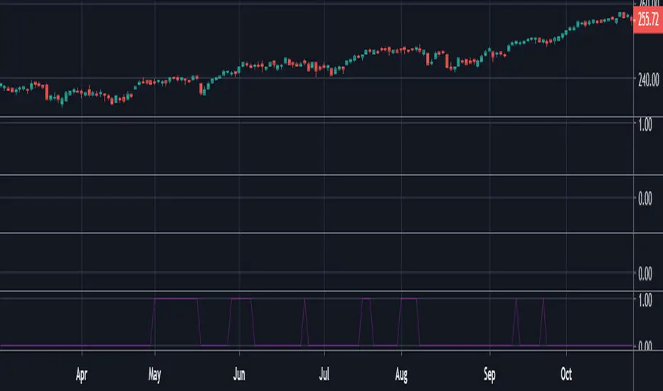
Trading Range Indicator - TRISimple script made to identify trading ranges in any timeframe
The oscillator bounces between 1 and 0. 1 means that the current asset is in a trading range and 0 meaning it is not.
The determination of a trading range is determined by the following:
ATR(14)40 and RSI<60
ADX<25
Due to all 3 having to be fulfilled in order for the oscillator to show there is a trading range, this causes a problem where 2 of the conditions are fulfilled and therefore still shows 0 on the oscillator, however, the asset could very well be in a trading range.
So what in the world do you use this for if there is such a significant margin of error?
Since all 3 conditions need to be fulfilled in order for it to be considered a trading range, this gives a very strong indicator of said trading ranges. So if a person is looking at individual stock tickers or the SPY index ticker, then when the oscillator reads a 1, it could be ideal to open an Iron Condor on said ticker. This means that this indicator is not well suiting for traditional long and short stock positions, but rather it is made for options traders who by using an Iron Condor can make money of a range-bound market.
Acc/Dist. Cloud with Fractal Deviation Bands by @XeL_ArjonaACCUMULATION / DISTRIBUTION CLOUD with MORPHIC DEVIATION BANDS
Ver. 2.0.beta.23:08:2015
by Ricardo M. Arjona @XeL_Arjona
DISCLAIMER
The Following indicator/code IS NOT intended to be a formal investment advice or recommendation by the author, nor should be construed as such. Users will be fully responsible by their use regarding their own trading vehicles/assets.
The embedded code and ideas within this work are FREELY AND PUBLICLY available on the Web for NON LUCRATIVE ACTIVITIES and must remain as is.
Pine Script code MOD's and adaptations by @XeL_Arjona with special mention in regard of:
Buy (Bull) and Sell (Bear) "Power Balance Algorithm by Vadim Gimelfarb published at Stocks & Commodities V. 21:10 (68-72).
Custom Weighting Coefficient for Exponential Moving Average (nEMA) adaptation work by @XeL_Arjona with contribution help from @RicardoSantos at TradingView @pinescript chat room.
Morphic Numbers (PHI & Plastic) Pine Script adaptation from it's algebraic generation formulas by @XeL_Arjona
Fractal Deviation Bands idea by @XeL_Arjona
CHANGE LOG:
ACCUMULATION / DISTRIBUTION CLOUD: I decided to change it's name from the Buy to Sell Pressure. The code is essentially the same as older versions and they are the center core (VORTEX?) of all derived New stuff which are:
MORPHIC NUMBERS: The "Golden Ratio" expressed by the result of the constant "PHI" and the newer and same in characteristics "Plastic Number" expressed as "PN". For more information about this regard take a look at: HERE!
CUSTOM(K) EXPONENTIAL MOVING AVERAGE: Some code has cleaned from last version to include as custom function the nEMA , which use an additional input (K) to customise the way the "exponentially" is weighted from the custom array. For the purpose of this indicator, I implement a volatility algorithm using the Average True Range of last 9 periods multiplied by the morphic number used in the fractal study. (Golden Ratio as default) The result is very similar in response to classic EMA but tend to accelerate or decelerate much more responsive with wider bars presented in trending average.
FRACTAL DEVIATION BANDS: The main idea is based on the so useful Standard Deviation process to create Bands in favor of a multiplier (As John Bollinger used in it's own bands) from a custom array, in which for this case is the "Volume Pressure Moving Average" as the main Vortex for the "Fractallitly", so then apply as many "Child bands" using the older one as the new calculation array using the same morphic constant as multiplier (Like Fibonacci but with other approach rather than %ratios). Results are AWSOME! Market tend to accelerate or decelerate their Trend in favor of a Fractal approach. This bands try to catch them, so please experiment and feedback me your own observations.
EXTERNAL TICKER FOR VOLUME DATA: I Added a way to input volume data for this kind of study from external tickers. This is just a quicky-hack given that currently TradingView is not adding Volume to their Indexes so; maybe this is temporary by now. It seems that this part of the code is conflicting with intraday timeframes, so You are advised.
This CODE is versioned as BETA FOR TESTING PROPOSES. By now TradingView Admins are changing lot's of things internally, so maybe this could conflict with correct rendering of this study with special tickers or timeframes. I will try to code by itself just the core parts of this study in order to use them at discretion in other areas. ALL NEW IDEAS OR MODIFICATIONS to these indicator(s) are Welcome in favor to deploy a better and more accurate readings. I will be very glad to be notified at Twitter or TradingView accounts at: @XeL_Arjona

ATR Risk Display - Multi FuturesWhat This Does
I got tired of manually calculating my ATR stops and risk for different futures contracts, especially when switching between ES, NQ, and their micro versions. This indicator automatically detects what futures symbol you're trading and shows you the exact tick count and dollar risk for your stop loss.
The Problem It Solves
If you trade futures with ATR-based stops, you know the hassle:
Different contracts have different tick values
You need to calculate position risk in dollars
Switching between symbols means redoing all the math
Renko charts make it even more confusing since ATR needs to come from regular candles
This handles all of that automatically.
Key Features
Auto-detects futures symbols - ES, NQ, YM, RTY, GC, CL, and all the micros (MES, MNQ, etc.)
Shows everything you need in one line: ATR(timeframe) × multiplier = X ticks ($XXX)
Works on Renko charts - pulls ATR from regular timeframe charts (super important if you use Renko)
Adjustable position sizing - set your contract count and see total risk instantly
Clean, minimal display - just the info you need, no clutter
How to Use
Add it to any futures chart
Set your preferred ATR timeframe (I use 5-minute)
Set your ATR multiplier (I use 1.5x for my stops)
Set your contract size
That's it - the indicator handles the rest
The display will show something like: "ES ATR(5) × 1.5 = 12 ticks ($150)"
Settings Explained
ATR Timeframe: What timeframe to calculate ATR from (always uses regular candles, even on Renko)
ATR Multiplier: How many ATRs for your stop (1.5 is common, 2.0 for wider stops)
Number of Contracts: Your position size for risk calculation
Auto-Detect Symbol: Leave on unless you want to manually override
Supported Futures
Full size: ES, NQ, YM, RTY, GC, CL, ZB, ZN, 6E, 6J
Micros: MES, MNQ, MYM, M2K, MGC, MCL
Notes
Made this primarily for my own ES trading but figured others might find it useful
The tick values are based on standard CME specs
If you trade other futures, you can modify the code to add them
Works great alongside level indicators for risk management
Why This Exists
I use ATR trailing stops on all my trades and got tired of doing mental math every time I switched between charts or contracts. Especially useful if you trade both full-size and micro contracts - the risk difference is huge and easy to mess up.
Hope this helps your trading! Feel free to suggest improvements.

Michael's FVG Detector═══════════════════════════════════════
Michael's FVG Detector
═══════════════════════════════════════
A clean and efficient Fair Value Gap (FVG) indicator for TradingView that helps traders identify market imbalances with precision.
───────────────────────────────────────
Overview
───────────────────────────────────────
Fair Value Gaps (FVGs) are price inefficiencies that occur when there's a gap between the wicks of candlesticks, indicating rapid price movement with minimal trading activity. These gaps often act as support/resistance zones where price may return to "fill the gap."
This indicator automatically detects and visualizes both bullish and bearish FVGs on any timeframe, making it easy to spot potential trading opportunities.
───────────────────────────────────────
Features
───────────────────────────────────────
Core Functionality
Automatic FVG Detection : Identifies Fair Value Gaps in real-time as they form
Bullish & Bearish FVGs : Detects both upward and downward price gaps
3-Candle Pattern : Uses classic FVG logic (current candle low > high from 2 bars ago for bullish, vice versa for bearish)
Gap Size Display : Shows the exact size of each FVG in ticks directly on the box
Confirmed Bars Only : Only draws FVGs on confirmed bars to prevent repainting
Customization
Color Settings : Fully customizable colors for bullish and bearish FVGs with transparency control
Text Color : Configurable color for the tick size labels
Default Styling : Comes with sensible defaults (20% transparency, dark gray labels)
Performance Optimization
Smart Cleanup : Automatically removes boxes outside the visible chart area
Efficient Rendering : Maintains optimal performance even on lower timeframes
No Repainting : Uses confirmed bars only for reliable signals
───────────────────────────────────────
How It Works
───────────────────────────────────────
Detection Logic
Bullish FVG:
Current bar's low is higher than the high from 2 bars ago
Creates an upward gap that price left behind during bullish momentum
Bearish FVG:
Current bar's high is lower than the low from 2 bars ago
Creates a downward gap that price left behind during bearish momentum
Visual Display
Each detected FVG is displayed as:
A semi-transparent colored box spanning the gap area
The box extends from bar -2 to the current bar
Gap size in ticks shown at the bottom-left of each box
Singular/plural formatting ("1 tick" vs "X ticks")
───────────────────────────────────────
Performance Notes
───────────────────────────────────────
Cleanup runs every 50 bars to maintain optimal performance
Only creates boxes on confirmed bars (no real-time repainting)
Efficiently manages memory by removing off-screen boxes
Suitable for both manual and automated trading strategies
───────────────────────────────────────
Disclaimer
───────────────────────────────────────
This indicator is for educational and informational purposes only. It is not financial advice. Always do your own research and risk management before making trading decisions.
───────────────────────────────────────
Author : Michael
Version : 1.0
License : Free for personal use
Last Updated : November 2025

Info de Vela 1m1-Minute Candle Info Dashboard (Real-Time)
Overview
This is a lightweight, real-time dashboard designed specifically for 1-minute (1m) scalping. It provides critical, non-lagging data about the current 1-minute candle, helping you make split-second decisions on stop-loss placement and risk assessment.The table updates on every tick without flickering or repainting.
Key Features (Real-Time Table)
The dashboard displays three key metrics about the current 1m candle:Time Remaining: A simple countdown timer showing the exact seconds remaining until the current candle closes (e.g., "00:34").Dist. to Extreme (Ticks): This is the core function for scalping. It calculates the distance (in ticks) from the current price to the furthest extreme of the candle (i.e., max(high - close, close - low)). This is ideal for traders who base their stop-loss on the current candle's range.Total Candle Range (Ticks): Displays the full high-to-low range of the current candle in ticks, giving you an instant read on volatility.
How to Use
This tool is designed to solve one problem: speed.Instead of manually measuring the distance for your stop-loss on every candle, you can instantly read the exact tick value from the table. This allows you to calculate your position size (lotage) much faster, which is essential in a fast-moving 1m environment.
REQUIREMENT:This indicator is designed to work ONLY on the 1-minute (1m) timeframe. It will display an error and show no data on any other chart.

Enhanced MA Crossover Pro📝 Strategy Summary: Enhanced MA Crossover Pro
This strategy is an advanced, highly configurable moving average (MA) crossover system designed for algorithmic trading. It uses the crossover of two customizable MAs (a "Fast" MA 1 and a "Slow" MA 2) as its core entry signal, but aggressively integrates multiple technical filters, time controls, and dynamic position management to create a robust and comprehensive trading system.
💡 Core Logic
Entry Signal: A bullish crossover (MA1 > MA2) generates a Long signal, and a bearish crossover (MA1 < MA2) generates a Short signal. Users can opt to use MA crossovers from a Higher Timeframe (HTF) for the entry signal.
Confirmation/Filters: The basic MA cross signal is filtered by several optional indicators (see Filters section below) to ensure trades align with a broader trend or momentum context.
Position Management: Trades are managed with a sophisticated system of Stop Loss, Take Profit, Trailing Stops, and Breakeven stops that can be fixed, ATR-based, or dynamically adjusted.
Risk Management: Daily limits are enforced for maximum profit/loss and maximum trades per day.
⚙️ Key Features and Customization
1. Moving Averages
Primary MAs (MA1 & MA2): Highly configurable lengths (default 8 & 20) and types: EMA, WMA, SMA, or SMMA/RMA.
Higher Timeframe (HTF) MAs: Optional MAs calculated on a user-defined resolution (e.g., "60" for 1-hour) for use as an entry signal or as a trend confirmation filter.
2. Multi-Filter System
The entry signal can be filtered by the following optional conditions:
SMA Filter: Price must be above a 200-period SMA for long trades, and below it for short trades.
VWAP Filter: Price must be above VWAP for long trades, and below it for short trades.
RSI Filter: Long trades are blocked if RSI is overbought (default 70); short trades are blocked if RSI is oversold (default 30).
MACD Filter: Requires the MACD Line to be above the Signal Line for long trades (and vice versa for short trades).
HTF Confirmation: Requires the HTF MA1 to be above HTF MA2 for long entries (and vice versa).
3. Dynamic Stop and Target Management (S/L & T/P)
The strategy provides extensive control over exits:
Stop Loss Methods:
Fixed: Fixed tick amount.
ATR: Based on a multiple of the Average True Range (ATR).
Capped ATR: ATR stop limited by a maximum fixed tick amount.
Exit on Close Cross MA: Position is closed if the price crosses back over the chosen MA (MA1 or MA2).
Breakeven Stop: A stop can be moved to the entry price once a trigger distance (fixed ticks or Adaptive Breakeven based on ATR%) is reached.
Trailing Stop: Can be fixed or ATR-based, with an optional feature to auto-tighten the trailing multiplier after the breakeven condition is met.
Profit Target: Can be a fixed tick amount or a dynamic target based on an ATR multiplier.
4. Time and Session Control
Trading Session: Trades are only taken between defined Start/End Hours and Minutes (e.g., 9:30 to 16:00).
Forced Close: All open positions are closed near the end of the session (e.g., 15:45).
Trading Days: Allows specific days of the week to be enabled or disabled for trading.
5. Risk and Position Limits
Daily Profit/Loss Limits: The strategy tracks daily realized and unrealized PnL in ticks and will close all positions and block new entries if the user-defined maximum profit or maximum loss is hit.
Max Trades Per Day: Limits the number of executed trades in a single day.
🎨 Outputs and Alerts
Plots: Plots the MA1, MA2, SMA, VWAP, and HTF MAs (if enabled) on the chart.
Shapes: Plots visual markers (BUY/SELL labels) on the bar where the MA crossover occurs.
Trailing Stop: Plots the dynamic trailing stop level when a position is open.
Alerts: Generates JSON-formatted alerts for entry ({"action":"buy", "price":...}) and exit ({"action":"exit", "position":"long", "price":...}).

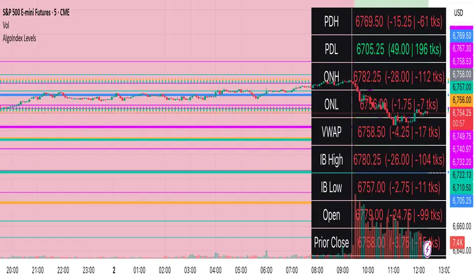
RTH Levels: VWAP + PDH/PDL + ONH/ONL + IBAlgo Index — Levels Pro (ONH/ONL • PDH/PDL • VWAP±Bands • IB • Gaps)
Purpose. A session-aware, non-repainting levels tool for intraday decision-making. Designed for futures and indices, with clean visuals, alerts, and a one-click Minimal Mode for screenshot-ready charts.
What it plots
• PDH/PDL (RTH-only) – Prior Regular Trading Hours high/low, computed intraday and frozen at the RTH close (no 24h mix-ups, no repainting).
• ONH/ONL – Prior Overnight high/low, held throughout RTH.
• RTH VWAP with ±σ bands – Volume-weighted variance, reset each RTH.
• Initial Balance (IB) – First N minutes of RTH, plus 1.5× / 2.0× extensions after IB completes.
• Today’s RTH Open & Prior RTH Close – With gap detection and “gap filled” alert.
• Killzone shading – NY Open (09:30–10:30 ET) and Lunch (11:15–13:30 ET).
• Values panel (top-right) – Each level with live distance in points & ticks.
• Right-edge level tags – With anti-overlap (stagger + vertical jitter).
• Price-scale tags – Native trackprice markers that always “stick” to the axis.
⸻
New in v6.4
• Minimal Mode: one click for a clean look (thinner lines, VWAP bands/IB extensions hidden, on-chart right-edge labels off; price-scale tags remain).
• Theme presets: Dark Hi-Contrast / Light Minimal / Futures Classic / Muted Dark.
• Anti-overlap controls: horizontal staggering, vertical jitter, and baseline offset to keep tags readable even when levels cluster.
⸻
Quick start (2 minutes)
1. Add to chart → keep defaults.
2. Sessions (ET):
• RTH Session default: 09:30–16:00 (US equities cash hours).
• Overnight Session default: 18:00–09:29.
Adjust for your market if you use different “day” hours (e.g., many use 08:20–13:30 ET for COMEX Gold).
3. Theme & Minimal Mode: pick a Theme Preset; enable Minimal Mode for screenshots.
4. Visibility: toggle PD/ON/VWAP/IB/References/Panel to taste.
5. Right-edge labels: turn Show Right-Edge Labels on. If they crowd, tune:
• Anti-overlap: min separation (ticks)
• Horizontal offset per tag (bars)
• Vertical jitter per step (ticks)
• Right-edge baseline offset (bars)
6. Alerts: open Add alert → Condition: and pick the events you want.
⸻
How levels are computed (no repainting)
• PDH/PDL: Intraday H/L are accumulated only while in RTH and saved at RTH close for “yesterday’s” values.
• ONH/ONL: Accumulated across the defined Overnight window and then held during RTH.
• RTH VWAP & ±σ: Volume-weighted mean and standard deviation, reset at the RTH open.
• IB: First N minutes of RTH (default 60). Extensions (1.5×/2.0×) appear after IB completes.
• Gaps: Today’s RTH open vs prior RTH close; “Gap Filled” triggers when price trades back to prior close.
⸻
Practical playbooks (how to trade around the levels)
1) PDH/PDL interactions
• Rejection: Price taps PDH/PDL then closes back inside → mean-reversion toward VWAP/IB.
• Acceptance: Close/hold beyond PDH/PDL with momentum → continuation to next HTF/IB target.
• Alert: PD Touch/Break.
2) ONH/ONL “taken”
• Often one ON extreme is taken during RTH. ONH Taken / ONL Taken → check if it’s a clean break or sweep & reclaim.
• Sweep + reclaim near VWAP can fuel rotations through the ON range.
3) VWAP ±σ framework
• Balanced: First tag of ±1σ often reverts toward VWAP.
• Trend: Persistent trade beyond ±1σ + IB break → target ±2σ/±3σ.
• Alerts: VWAP Cross and VWAP Reject (cross then immediate fail back).
4) IB breaks
• After IB completes, a clean IB break commonly targets 1.5× and sometimes 2.0×.
• Quick return inside IB = possible fade back to the opposite IB edge/VWAP.
• Alerts: IB Break Up / Down.
5) Gaps
• Gap-and-go: Opening drive away from prior close + VWAP support → trend until IB completion.
• Gap-fill: Weak open and VWAP overhead/underfoot → trade toward prior close; manage on Gap Filled alert.
Pro tip: Stack confluences (e.g., ONL sweep + VWAP reclaim + IB hold) and respect your execution rules (e.g., require a 5-minute close in direction, or your order-flow confirmation).
⸻
Inputs you’ll actually touch
• Sessions (ET): Session Timezone, RTH Session, Overnight Session.
• Visibility: toggles for PD/ON/VWAP/IB/Ref/Panel.
• VWAP bands: set σ multipliers (±1/±2/±3).
• IB: duration (minutes) and extension multipliers (1.5× / 2.0×).
• Style & Theme: Theme Preset, Main Line Width, Trackprice, Minimal Mode, and anti-overlap controls.
⸻
Alerts included
• PD Touch/Break — High ≥ PDH or Low ≤ PDL
• ONH Taken / ONL Taken — First in-RTH take of ONH/ONL
• VWAP Cross — Close crosses VWAP
• VWAP Reject — Cross then immediate fail back
• IB Break Up / Down — Break of IB High/Low after IB completes
• Gap Filled — Price trades back to prior RTH close
Setup: Add alert → Condition: Algo Index — Levels Pro → choose event → message → Notify on app/email.
⸻
Panel guide
The top-right panel shows each level plus live distance from last price:
LevelValue (Δpoints | Δticks)
Coloring: green if level is below current price, red if above.
⸻
Styling & screenshot tips
• Use Theme Preset that matches your chart.
• For dark charts, “Dark Hi-Contrast” with Main Line Width = 3 works well.
• Enable Trackprice for crisp axis tags that always stick to the right edge.
• Turn on Minimal Mode for cleaner screenshots (no VWAP bands or IB extensions, on-chart tags off; price-scale tags remain).
• If tags crowd, increase min separation (ticks) to 30–60 and horizontal offset to 3–5; add vertical jitter (4–12 ticks) and/or push tags farther right with baseline offset (bars).
⸻
Behavior & limitations
• Levels are computed incrementally; tables refresh on the last bar for efficiency.
• Right-edge labels are placed at bar_index + offset and do not track extra right-margin scrolling (TradingView limitation). The price-scale tags (from trackprice) do track the axis.
• “RTH” is what you define in inputs. If your market uses different day hours, change the session strings so PDH/PDL reflect your definition of “yesterday’s session.”
⸻
FAQ
Q: My PDH/PDL don’t match the daily chart.
A: By design this uses RTH-only highs/lows, not 24h daily bars. Adjust sessions if you want a different definition.
Q: Right-edge tags overlap or don’t sit at the far right.
A: Increase min separation / horizontal offset / vertical jitter and/or push tags farther with baseline offset. If you want markers that always hug the axis, rely on Trackprice.
Q: Can I change killzones?
A: Yes—edit the session strings in settings or request a version with user inputs for custom windows.
⸻
Disclaimer
Educational use only. This is not financial advice. Always apply your own risk management and confirmation rules.
⸻
Enjoy it? Please ⭐ the script and share screenshots using Minimal Mode + a Theme Preset that fits your style.
NightWatch 24/5 [theUltimator5]NightWatch 24/5 is a comprehensive indicator designed to seamlessly display both regular and overnight trading (BOATS exchange) into a single chart. Current TV limitations don't allow both overnight trading and regular exchanges to appear on the same chart due to timeframe visibility settings. We can either select between RTH (Regular Trading Hours) or ETH (Extended Trading Hours). There is no option to show 24 hour charts when looking at a stock. This indicator attempts to solve this issue.
Please read the entire description thoroughly because this indicator takes a little bit of setup to work properly!
---IMPORTANT-- -
This indicator MUST be used over a liquid cryptocurrency chart, like Bitcoin. It requires access to something that trades 24/7 and has volume data for all periods. Bitcoin on Coinbase is the best option. Please select Bitcoin as your main ticker before adding this indicator to the chart.
-------------------
This indicator combines the price of both the regular trading hours and the overnight trading to create a single price line and volume candles. You can select view settings to either overlay the price on the chart, or have it below the chart. Volume can be toggled on or off as well.
Default settings:
Ticker = GME
Overlay Candles on Main Chart = true
Display Data = Both Price and Volume
Show Status Table = true
Here is an explanation for each of these settings:
Ticker - Type in the ticker you want to track overnight and intraday data for
Overlay Candles on Main chart - This will push the price candles onto the main chart area instead of below it. Volume candles will remain in their own separate pane below. This is useful if you want to track both price and volume without adding the indicator twice.
Display Data - This determines what data to show. Volume, price, or both volume and price.
Show Status Table - This toggles on or off the table that shows the ticker name, current session, and the price (change) of the ticker since the most recent daily close.
If you overlay the price onto the chart, the price of the stock you are looking at will likely be a VERY different price than the crypto it is overlaying against. There are a couple workarounds. You can either zoom into the chart around the price of the stock you are looking at (time consuming), or you can go into your object tree and drag the indicator up into the main chart area. This will overlay the price onto the crypto while maintaining it's own unique y-axis.
After you move the indicator up, you can add the indicator back a second time, then change the settings to only show the volume candles. You can then toggle off the table on one of the two so you don't see duplicate tables. This is the setting I am showing in my chart above. The indicator is added twice with the price being pulled up into the same window as Bitcoin, then a second instance below showing just volume.
--LIMITATIONS--
Since the indicator requires the use of a 24 hour market ticker like Bitcoin, it DOES NOT display extended hours data. The price and volume data STOPS at 16:00 EST then resumes back up at 20:00 EST when BOATS opens. At 04:00, the price and volume then stops until 09:30, when the regular trading hours begin. This causes a flat line in the price during those periods. Unfortunately, there is no current workaround to this issue.
If Bitcoin becomes illiquid (or whatever crypto you choose), it will only populate data for the ticker you want if there is data available for that crypto at the same time period. A gap in Bitcoin volume will show a gap in trade activity for your ticker.

LTA - Futures Contract Size CalculatorLTA - Futures Contract Size Calculator
This indicator helps futures traders calculate the potential stop-loss (SL) value for their trades with ease. Simply input your entry price, stop-loss price, and number of contracts, and the indicator will compute the ticks moved, price movement, and total SL value in USD.
Key Features:
Supports a wide range of futures contracts, including:
Index Futures: E-mini S&P 500 (ES), Micro E-mini S&P 500 (MES), E-mini Nasdaq-100 (NQ), Micro E-mini Nasdaq-100 (MNQ)
Commodity Futures: Crude Oil (CL), Gold (GC), Micro Gold (MGC), Silver (SI), Micro Silver (SIL), Platinum (PL), Micro Platinum (MPL), Natural Gas (NG), Micro Natural Gas (MNG)
Bond Futures: 30-Year T-Bond (ZB)
Currency Futures: Euro FX (6E), Japanese Yen (6J), Australian Dollar (6A), British Pound (6B), Canadian Dollar (6C), Swiss Franc (6S), New Zealand Dollar (6N)
Displays key metrics in a clean table (bottom-right corner):
Instrument, Entry Price, Stop-Loss Price, Number of Contracts, Tick Size, Ticks Moved, Price Movement, and Total SL Value.
Automatically calculates based on the selected instrument’s tick size and tick value.
User-friendly interface with a dark theme for better visibility.
How to Use:
Add the indicator to your chart.
Select your instrument from the dropdown (ensure it matches your chart’s symbol, e.g., "NG1!" for NATURAL GAS (NG)).
Input your Entry Price, Stop-Loss Price, and Number of Contracts.
View the results in the table, including the Total SL Value in USD.
Ideal For:
Futures traders looking to quickly assess stop-loss risk.
Beginners and pros trading indices, commodities, bonds, or currencies.
Note: Ensure your chart symbol matches the selected instrument for accurate calculations. For best results, test with a few contracts and price levels to confirm the output.
This description is tailored for TradingView’s audience, providing a clear overview of the indicator’s functionality, supported instruments, and usage instructions. It also includes a note to help users avoid common pitfalls (e.g., mismatched symbols). If you’d like to adjust the tone, add more details, or include specific TradingView tags (e.g., , ), let me know!

E9 MM Nuke signalScript identifies wickless candles on a specified higher timeframe and plots them on a lower timeframe (If desired), such as 15 minutes. It includes options to adjust the margin for error (e.g. 5 tick wick), higher timeframe, and toggle the volume filter with period adjustment.
Wickless candles signal strong market sentiment shifts, indicating areas of significant buying or selling pressure. These areas can become key levels of support or resistance, making them crucial to monitor for potential price revisits.
Why Price Revisits Wickless Areas
Manipulators often create artificial wickless candles to deceive traders. However, genuine market movements can also produce wickless candles, indicating a strong consensus among market participants. In either case, the price is likely to revisit these areas as traders and investors react to the perceived market sentiment shift.
Key Features:
Margin Input:
Description: Allows users to specify the margin in 0.01 tick increments to account for small wicks due to spread issues.
Example: A margin of 0.05 ticks means the script will consider candles wickless if the high is within 0.05 ticks of the open and the low is within 0.05 ticks of the open.
Volume Filter:
Description: Users can enable or disable a volume filter to consider only candles with a volume greater than the average volume over a specified period.
Default: Enabled by default.
Volume Period Input: Users can specify the period for calculating the average volume (e.g., 9 periods).
Higher Timeframe Input:
Description: Allows users to select the higher timeframe on which to identify wickless candles.
Options: H4 ("240"), Daily ("D"), Weekly ("W"), Monthly ("M").
Plotting:
Bearish Wickless Candles: Plotted with a red circle and a "🐻" emoji above the bar.
Bullish Wickless Candles: Plotted with a green circle and a "🐂" emoji below the bar.

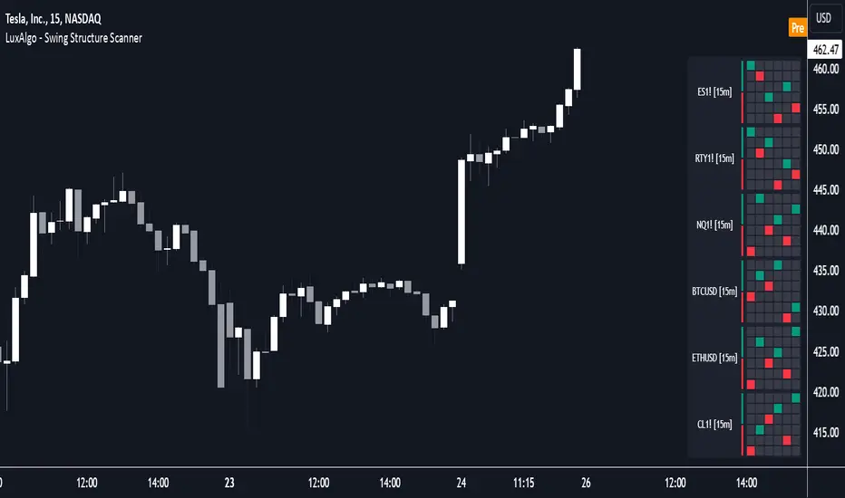
Swing Structure Scanner [LuxAlgo]The Swing Structure Scanner Indicator is a dashboard type indicator which displays a Consolidated "High/Low-Only" view of swing structure, with the capability to retrieve and display swing points from up to 6 different tickers and timeframes at once.
🔶 USAGE
This indicator displays swing structure data from up to 6 unique tickers or timeframes; Each graph represents the current swing structure retrieved from the requested chart/s.
Each swing graph displays the current live swing point positioning relative to the previous swing points. By analyzing the different formations, patterns can more easily be recognized and found across multiple tickers or timeframes at once.
This indicator serves as a nifty tool for confluence recognition, whether that's confluence throughout market tickers, or confluence through higher timeframes on the same ticker.
Alternatively, viewing the relative positioning of each swing point to each other, should give a clearer idea when higher lows or lower highs are formed. This can potentially indicate a newly forming trend, as well as serving as a warning to watch for breakouts.
The swing length can be changed to align with each individual's strategy, as well as a display look back can be adjusted to show more or less swing points at one time.
The display is fairly customizable, it is not fixed to 6 symbols at all times and can be minimized to only display the number of symbols needed; Additionally, the display can be set to vertical mode or horizontal(default) to utilize as needed.
Note: Hover over the swing point in the dashboard to get a readout of the exact price level of the swing point.
🔶 SETTINGS
Swing Length: Set the swing length for the structure calculations.
Swing Display Lookback: Sets the number of swing points (Pairs) to display in each Swing Graph display.
Symbols: Sets the Timeframe and Symbol for each Swing Graph.
Vertical Display: Display the Swing Graphs up and down, rather than side to side.
Scaling Factor: Scales the entire indicator up or down, to fit your needs.
Universal Ratio Trend Matrix [InvestorUnknown]The Universal Ratio Trend Matrix is designed for trend analysis on asset/asset ratios, supporting up to 40 different assets. Its primary purpose is to help identify which assets are outperforming others within a selection, providing a broad overview of market trends through a matrix of ratios. The indicator automatically expands the matrix based on the number of assets chosen, simplifying the process of comparing multiple assets in terms of performance.
Key features include the ability to choose from a narrow selection of indicators to perform the ratio trend analysis, allowing users to apply well-defined metrics to their comparison.
Drawback: Due to the computational intensity involved in calculating ratios across many assets, the indicator has a limitation related to loading speed. TradingView has time limits for calculations, and for users on the basic (free) plan, this could result in frequent errors due to exceeded time limits. To use the indicator effectively, users with any paid plans should run it on timeframes higher than 8h (the lowest timeframe on which it managed to load with 40 assets), as lower timeframes may not reliably load.
Indicators:
RSI_raw: Simple function to calculate the Relative Strength Index (RSI) of a source (asset price).
RSI_sma: Calculates RSI followed by a Simple Moving Average (SMA).
RSI_ema: Calculates RSI followed by an Exponential Moving Average (EMA).
CCI: Calculates the Commodity Channel Index (CCI).
Fisher: Implements the Fisher Transform to normalize prices.
Utility Functions:
f_remove_exchange_name: Strips the exchange name from asset tickers (e.g., "INDEX:BTCUSD" to "BTCUSD").
f_remove_exchange_name(simple string name) =>
string parts = str.split(name, ":")
string result = array.size(parts) > 1 ? array.get(parts, 1) : name
result
f_get_price: Retrieves the closing price of a given asset ticker using request.security().
f_constant_src: Checks if the source data is constant by comparing multiple consecutive values.
Inputs:
General settings allow users to select the number of tickers for analysis (used_assets) and choose the trend indicator (RSI, CCI, Fisher, etc.).
Table settings customize how trend scores are displayed in terms of text size, header visibility, highlighting options, and top-performing asset identification.
The script includes inputs for up to 40 assets, allowing the user to select various cryptocurrencies (e.g., BTCUSD, ETHUSD, SOLUSD) or other assets for trend analysis.
Price Arrays:
Price values for each asset are stored in variables (price_a1 to price_a40) initialized as na. These prices are updated only for the number of assets specified by the user (used_assets).
Trend scores for each asset are stored in separate arrays
// declare price variables as "na"
var float price_a1 = na, var float price_a2 = na, var float price_a3 = na, var float price_a4 = na, var float price_a5 = na
var float price_a6 = na, var float price_a7 = na, var float price_a8 = na, var float price_a9 = na, var float price_a10 = na
var float price_a11 = na, var float price_a12 = na, var float price_a13 = na, var float price_a14 = na, var float price_a15 = na
var float price_a16 = na, var float price_a17 = na, var float price_a18 = na, var float price_a19 = na, var float price_a20 = na
var float price_a21 = na, var float price_a22 = na, var float price_a23 = na, var float price_a24 = na, var float price_a25 = na
var float price_a26 = na, var float price_a27 = na, var float price_a28 = na, var float price_a29 = na, var float price_a30 = na
var float price_a31 = na, var float price_a32 = na, var float price_a33 = na, var float price_a34 = na, var float price_a35 = na
var float price_a36 = na, var float price_a37 = na, var float price_a38 = na, var float price_a39 = na, var float price_a40 = na
// create "empty" arrays to store trend scores
var a1_array = array.new_int(40, 0), var a2_array = array.new_int(40, 0), var a3_array = array.new_int(40, 0), var a4_array = array.new_int(40, 0)
var a5_array = array.new_int(40, 0), var a6_array = array.new_int(40, 0), var a7_array = array.new_int(40, 0), var a8_array = array.new_int(40, 0)
var a9_array = array.new_int(40, 0), var a10_array = array.new_int(40, 0), var a11_array = array.new_int(40, 0), var a12_array = array.new_int(40, 0)
var a13_array = array.new_int(40, 0), var a14_array = array.new_int(40, 0), var a15_array = array.new_int(40, 0), var a16_array = array.new_int(40, 0)
var a17_array = array.new_int(40, 0), var a18_array = array.new_int(40, 0), var a19_array = array.new_int(40, 0), var a20_array = array.new_int(40, 0)
var a21_array = array.new_int(40, 0), var a22_array = array.new_int(40, 0), var a23_array = array.new_int(40, 0), var a24_array = array.new_int(40, 0)
var a25_array = array.new_int(40, 0), var a26_array = array.new_int(40, 0), var a27_array = array.new_int(40, 0), var a28_array = array.new_int(40, 0)
var a29_array = array.new_int(40, 0), var a30_array = array.new_int(40, 0), var a31_array = array.new_int(40, 0), var a32_array = array.new_int(40, 0)
var a33_array = array.new_int(40, 0), var a34_array = array.new_int(40, 0), var a35_array = array.new_int(40, 0), var a36_array = array.new_int(40, 0)
var a37_array = array.new_int(40, 0), var a38_array = array.new_int(40, 0), var a39_array = array.new_int(40, 0), var a40_array = array.new_int(40, 0)
f_get_price(simple string ticker) =>
request.security(ticker, "", close)
// Prices for each USED asset
f_get_asset_price(asset_number, ticker) =>
if (used_assets >= asset_number)
f_get_price(ticker)
else
na
// overwrite empty variables with the prices if "used_assets" is greater or equal to the asset number
if barstate.isconfirmed // use barstate.isconfirmed to avoid "na prices" and calculation errors that result in empty cells in the table
price_a1 := f_get_asset_price(1, asset1), price_a2 := f_get_asset_price(2, asset2), price_a3 := f_get_asset_price(3, asset3), price_a4 := f_get_asset_price(4, asset4)
price_a5 := f_get_asset_price(5, asset5), price_a6 := f_get_asset_price(6, asset6), price_a7 := f_get_asset_price(7, asset7), price_a8 := f_get_asset_price(8, asset8)
price_a9 := f_get_asset_price(9, asset9), price_a10 := f_get_asset_price(10, asset10), price_a11 := f_get_asset_price(11, asset11), price_a12 := f_get_asset_price(12, asset12)
price_a13 := f_get_asset_price(13, asset13), price_a14 := f_get_asset_price(14, asset14), price_a15 := f_get_asset_price(15, asset15), price_a16 := f_get_asset_price(16, asset16)
price_a17 := f_get_asset_price(17, asset17), price_a18 := f_get_asset_price(18, asset18), price_a19 := f_get_asset_price(19, asset19), price_a20 := f_get_asset_price(20, asset20)
price_a21 := f_get_asset_price(21, asset21), price_a22 := f_get_asset_price(22, asset22), price_a23 := f_get_asset_price(23, asset23), price_a24 := f_get_asset_price(24, asset24)
price_a25 := f_get_asset_price(25, asset25), price_a26 := f_get_asset_price(26, asset26), price_a27 := f_get_asset_price(27, asset27), price_a28 := f_get_asset_price(28, asset28)
price_a29 := f_get_asset_price(29, asset29), price_a30 := f_get_asset_price(30, asset30), price_a31 := f_get_asset_price(31, asset31), price_a32 := f_get_asset_price(32, asset32)
price_a33 := f_get_asset_price(33, asset33), price_a34 := f_get_asset_price(34, asset34), price_a35 := f_get_asset_price(35, asset35), price_a36 := f_get_asset_price(36, asset36)
price_a37 := f_get_asset_price(37, asset37), price_a38 := f_get_asset_price(38, asset38), price_a39 := f_get_asset_price(39, asset39), price_a40 := f_get_asset_price(40, asset40)
Universal Indicator Calculation (f_calc_score):
This function allows switching between different trend indicators (RSI, CCI, Fisher) for flexibility.
It uses a switch-case structure to calculate the indicator score, where a positive trend is denoted by 1 and a negative trend by 0. Each indicator has its own logic to determine whether the asset is trending up or down.
// use switch to allow "universality" in indicator selection
f_calc_score(source, trend_indicator, int_1, int_2) =>
int score = na
if (not f_constant_src(source)) and source > 0.0 // Skip if you are using the same assets for ratio (for example BTC/BTC)
x = switch trend_indicator
"RSI (Raw)" => RSI_raw(source, int_1)
"RSI (SMA)" => RSI_sma(source, int_1, int_2)
"RSI (EMA)" => RSI_ema(source, int_1, int_2)
"CCI" => CCI(source, int_1)
"Fisher" => Fisher(source, int_1)
y = switch trend_indicator
"RSI (Raw)" => x > 50 ? 1 : 0
"RSI (SMA)" => x > 50 ? 1 : 0
"RSI (EMA)" => x > 50 ? 1 : 0
"CCI" => x > 0 ? 1 : 0
"Fisher" => x > x ? 1 : 0
score := y
else
score := 0
score
Array Setting Function (f_array_set):
This function populates an array with scores calculated for each asset based on a base price (p_base) divided by the prices of the individual assets.
It processes multiple assets (up to 40), calling the f_calc_score function for each.
// function to set values into the arrays
f_array_set(a_array, p_base) =>
array.set(a_array, 0, f_calc_score(p_base / price_a1, trend_indicator, int_1, int_2))
array.set(a_array, 1, f_calc_score(p_base / price_a2, trend_indicator, int_1, int_2))
array.set(a_array, 2, f_calc_score(p_base / price_a3, trend_indicator, int_1, int_2))
array.set(a_array, 3, f_calc_score(p_base / price_a4, trend_indicator, int_1, int_2))
array.set(a_array, 4, f_calc_score(p_base / price_a5, trend_indicator, int_1, int_2))
array.set(a_array, 5, f_calc_score(p_base / price_a6, trend_indicator, int_1, int_2))
array.set(a_array, 6, f_calc_score(p_base / price_a7, trend_indicator, int_1, int_2))
array.set(a_array, 7, f_calc_score(p_base / price_a8, trend_indicator, int_1, int_2))
array.set(a_array, 8, f_calc_score(p_base / price_a9, trend_indicator, int_1, int_2))
array.set(a_array, 9, f_calc_score(p_base / price_a10, trend_indicator, int_1, int_2))
array.set(a_array, 10, f_calc_score(p_base / price_a11, trend_indicator, int_1, int_2))
array.set(a_array, 11, f_calc_score(p_base / price_a12, trend_indicator, int_1, int_2))
array.set(a_array, 12, f_calc_score(p_base / price_a13, trend_indicator, int_1, int_2))
array.set(a_array, 13, f_calc_score(p_base / price_a14, trend_indicator, int_1, int_2))
array.set(a_array, 14, f_calc_score(p_base / price_a15, trend_indicator, int_1, int_2))
array.set(a_array, 15, f_calc_score(p_base / price_a16, trend_indicator, int_1, int_2))
array.set(a_array, 16, f_calc_score(p_base / price_a17, trend_indicator, int_1, int_2))
array.set(a_array, 17, f_calc_score(p_base / price_a18, trend_indicator, int_1, int_2))
array.set(a_array, 18, f_calc_score(p_base / price_a19, trend_indicator, int_1, int_2))
array.set(a_array, 19, f_calc_score(p_base / price_a20, trend_indicator, int_1, int_2))
array.set(a_array, 20, f_calc_score(p_base / price_a21, trend_indicator, int_1, int_2))
array.set(a_array, 21, f_calc_score(p_base / price_a22, trend_indicator, int_1, int_2))
array.set(a_array, 22, f_calc_score(p_base / price_a23, trend_indicator, int_1, int_2))
array.set(a_array, 23, f_calc_score(p_base / price_a24, trend_indicator, int_1, int_2))
array.set(a_array, 24, f_calc_score(p_base / price_a25, trend_indicator, int_1, int_2))
array.set(a_array, 25, f_calc_score(p_base / price_a26, trend_indicator, int_1, int_2))
array.set(a_array, 26, f_calc_score(p_base / price_a27, trend_indicator, int_1, int_2))
array.set(a_array, 27, f_calc_score(p_base / price_a28, trend_indicator, int_1, int_2))
array.set(a_array, 28, f_calc_score(p_base / price_a29, trend_indicator, int_1, int_2))
array.set(a_array, 29, f_calc_score(p_base / price_a30, trend_indicator, int_1, int_2))
array.set(a_array, 30, f_calc_score(p_base / price_a31, trend_indicator, int_1, int_2))
array.set(a_array, 31, f_calc_score(p_base / price_a32, trend_indicator, int_1, int_2))
array.set(a_array, 32, f_calc_score(p_base / price_a33, trend_indicator, int_1, int_2))
array.set(a_array, 33, f_calc_score(p_base / price_a34, trend_indicator, int_1, int_2))
array.set(a_array, 34, f_calc_score(p_base / price_a35, trend_indicator, int_1, int_2))
array.set(a_array, 35, f_calc_score(p_base / price_a36, trend_indicator, int_1, int_2))
array.set(a_array, 36, f_calc_score(p_base / price_a37, trend_indicator, int_1, int_2))
array.set(a_array, 37, f_calc_score(p_base / price_a38, trend_indicator, int_1, int_2))
array.set(a_array, 38, f_calc_score(p_base / price_a39, trend_indicator, int_1, int_2))
array.set(a_array, 39, f_calc_score(p_base / price_a40, trend_indicator, int_1, int_2))
a_array
Conditional Array Setting (f_arrayset):
This function checks if the number of used assets is greater than or equal to a specified number before populating the arrays.
// only set values into arrays for USED assets
f_arrayset(asset_number, a_array, p_base) =>
if (used_assets >= asset_number)
f_array_set(a_array, p_base)
else
na
Main Logic
The main logic initializes arrays to store scores for each asset. Each array corresponds to one asset's performance score.
Setting Trend Values: The code calls f_arrayset for each asset, populating the respective arrays with calculated scores based on the asset prices.
Combining Arrays: A combined_array is created to hold all the scores from individual asset arrays. This array facilitates further analysis, allowing for an overview of the performance scores of all assets at once.
// create a combined array (work-around since pinescript doesn't support having array of arrays)
var combined_array = array.new_int(40 * 40, 0)
if barstate.islast
for i = 0 to 39
array.set(combined_array, i, array.get(a1_array, i))
array.set(combined_array, i + (40 * 1), array.get(a2_array, i))
array.set(combined_array, i + (40 * 2), array.get(a3_array, i))
array.set(combined_array, i + (40 * 3), array.get(a4_array, i))
array.set(combined_array, i + (40 * 4), array.get(a5_array, i))
array.set(combined_array, i + (40 * 5), array.get(a6_array, i))
array.set(combined_array, i + (40 * 6), array.get(a7_array, i))
array.set(combined_array, i + (40 * 7), array.get(a8_array, i))
array.set(combined_array, i + (40 * 8), array.get(a9_array, i))
array.set(combined_array, i + (40 * 9), array.get(a10_array, i))
array.set(combined_array, i + (40 * 10), array.get(a11_array, i))
array.set(combined_array, i + (40 * 11), array.get(a12_array, i))
array.set(combined_array, i + (40 * 12), array.get(a13_array, i))
array.set(combined_array, i + (40 * 13), array.get(a14_array, i))
array.set(combined_array, i + (40 * 14), array.get(a15_array, i))
array.set(combined_array, i + (40 * 15), array.get(a16_array, i))
array.set(combined_array, i + (40 * 16), array.get(a17_array, i))
array.set(combined_array, i + (40 * 17), array.get(a18_array, i))
array.set(combined_array, i + (40 * 18), array.get(a19_array, i))
array.set(combined_array, i + (40 * 19), array.get(a20_array, i))
array.set(combined_array, i + (40 * 20), array.get(a21_array, i))
array.set(combined_array, i + (40 * 21), array.get(a22_array, i))
array.set(combined_array, i + (40 * 22), array.get(a23_array, i))
array.set(combined_array, i + (40 * 23), array.get(a24_array, i))
array.set(combined_array, i + (40 * 24), array.get(a25_array, i))
array.set(combined_array, i + (40 * 25), array.get(a26_array, i))
array.set(combined_array, i + (40 * 26), array.get(a27_array, i))
array.set(combined_array, i + (40 * 27), array.get(a28_array, i))
array.set(combined_array, i + (40 * 28), array.get(a29_array, i))
array.set(combined_array, i + (40 * 29), array.get(a30_array, i))
array.set(combined_array, i + (40 * 30), array.get(a31_array, i))
array.set(combined_array, i + (40 * 31), array.get(a32_array, i))
array.set(combined_array, i + (40 * 32), array.get(a33_array, i))
array.set(combined_array, i + (40 * 33), array.get(a34_array, i))
array.set(combined_array, i + (40 * 34), array.get(a35_array, i))
array.set(combined_array, i + (40 * 35), array.get(a36_array, i))
array.set(combined_array, i + (40 * 36), array.get(a37_array, i))
array.set(combined_array, i + (40 * 37), array.get(a38_array, i))
array.set(combined_array, i + (40 * 38), array.get(a39_array, i))
array.set(combined_array, i + (40 * 39), array.get(a40_array, i))
Calculating Sums: A separate array_sums is created to store the total score for each asset by summing the values of their respective score arrays. This allows for easy comparison of overall performance.
Ranking Assets: The final part of the code ranks the assets based on their total scores stored in array_sums. It assigns a rank to each asset, where the asset with the highest score receives the highest rank.
// create array for asset RANK based on array.sum
var ranks = array.new_int(used_assets, 0)
// for loop that calculates the rank of each asset
if barstate.islast
for i = 0 to (used_assets - 1)
int rank = 1
for x = 0 to (used_assets - 1)
if i != x
if array.get(array_sums, i) < array.get(array_sums, x)
rank := rank + 1
array.set(ranks, i, rank)
Dynamic Table Creation
Initialization: The table is initialized with a base structure that includes headers for asset names, scores, and ranks. The headers are set to remain constant, ensuring clarity for users as they interpret the displayed data.
Data Population: As scores are calculated for each asset, the corresponding values are dynamically inserted into the table. This is achieved through a loop that iterates over the scores and ranks stored in the combined_array and array_sums, respectively.
Automatic Extending Mechanism
Variable Asset Count: The code checks the number of assets defined by the user. Instead of hardcoding the number of rows in the table, it uses a variable to determine the extent of the data that needs to be displayed. This allows the table to expand or contract based on the number of assets being analyzed.
Dynamic Row Generation: Within the loop that populates the table, the code appends new rows for each asset based on the current asset count. The structure of each row includes the asset name, its score, and its rank, ensuring that the table remains consistent regardless of how many assets are involved.
// Automatically extending table based on the number of used assets
var table table = table.new(position.bottom_center, 50, 50, color.new(color.black, 100), color.white, 3, color.white, 1)
if barstate.islast
if not hide_head
table.cell(table, 0, 0, "Universal Ratio Trend Matrix", text_color = color.white, bgcolor = #010c3b, text_size = fontSize)
table.merge_cells(table, 0, 0, used_assets + 3, 0)
if not hide_inps
table.cell(table, 0, 1,
text = "Inputs: You are using " + str.tostring(trend_indicator) + ", which takes: " + str.tostring(f_get_input(trend_indicator)),
text_color = color.white, text_size = fontSize), table.merge_cells(table, 0, 1, used_assets + 3, 1)
table.cell(table, 0, 2, "Assets", text_color = color.white, text_size = fontSize, bgcolor = #010c3b)
for x = 0 to (used_assets - 1)
table.cell(table, x + 1, 2, text = str.tostring(array.get(assets, x)), text_color = color.white, bgcolor = #010c3b, text_size = fontSize)
table.cell(table, 0, x + 3, text = str.tostring(array.get(assets, x)), text_color = color.white, bgcolor = f_asset_col(array.get(ranks, x)), text_size = fontSize)
for r = 0 to (used_assets - 1)
for c = 0 to (used_assets - 1)
table.cell(table, c + 1, r + 3, text = str.tostring(array.get(combined_array, c + (r * 40))),
text_color = hl_type == "Text" ? f_get_col(array.get(combined_array, c + (r * 40))) : color.white, text_size = fontSize,
bgcolor = hl_type == "Background" ? f_get_col(array.get(combined_array, c + (r * 40))) : na)
for x = 0 to (used_assets - 1)
table.cell(table, x + 1, x + 3, "", bgcolor = #010c3b)
table.cell(table, used_assets + 1, 2, "", bgcolor = #010c3b)
for x = 0 to (used_assets - 1)
table.cell(table, used_assets + 1, x + 3, "==>", text_color = color.white)
table.cell(table, used_assets + 2, 2, "SUM", text_color = color.white, text_size = fontSize, bgcolor = #010c3b)
table.cell(table, used_assets + 3, 2, "RANK", text_color = color.white, text_size = fontSize, bgcolor = #010c3b)
for x = 0 to (used_assets - 1)
table.cell(table, used_assets + 2, x + 3,
text = str.tostring(array.get(array_sums, x)),
text_color = color.white, text_size = fontSize,
bgcolor = f_highlight_sum(array.get(array_sums, x), array.get(ranks, x)))
table.cell(table, used_assets + 3, x + 3,
text = str.tostring(array.get(ranks, x)),
text_color = color.white, text_size = fontSize,
bgcolor = f_highlight_rank(array.get(ranks, x)))

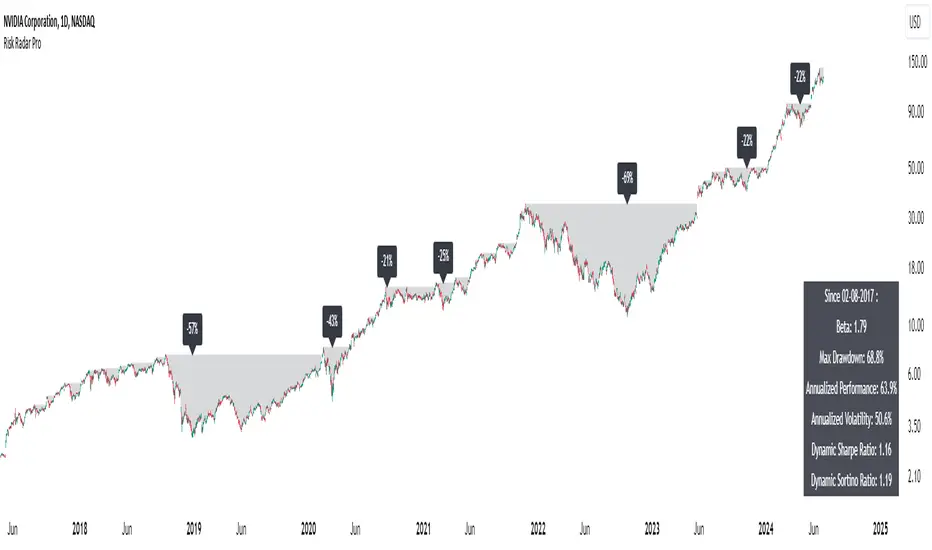
Risk Radar ProThe "Risk Radar Pro" indicator is a sophisticated tool designed to help investors and traders assess the risk and performance of their investments over a specified period. This presentation will explain each component of the indicator, how to interpret the results, and the advantages compared to traditional metrics.
The "Risk Radar Pro" indicator includes several key metrics:
● Beta
● Maximum Drawdown
● Compound Annual Growth Rate (CAGR)
● Annualized Volatility
● Dynamic Sharpe Ratio
● Dynamic Sortino Ratio
Each of these metrics is dynamically calculated using data from the entire selected period, providing a more adaptive and accurate measure of performance and risk.
1. Start Date
● Description: The date from which the calculations begin.
● Interpretation: This allows the user to set a specific period for analysis, ensuring that all metrics reflect the performance from this point onward.
2. Beta
● Description: Beta measures the volatility or systematic risk of the instrument relative to a reference index (e.g., SPY).
● Interpretation: A beta of 1 indicates that the instrument moves with the market. A beta greater than 1 indicates more volatility than the market, while a beta less than 1 indicates less volatility.
● Advantages: Unlike classic beta, which typically uses fixed historical intervals, this dynamic beta adjusts to market changes over the entire selected period, providing a more responsive measure.
3. Maximum Drawdown
● Description: The maximum observed loss from a peak to a trough before a new peak is achieved.
● Interpretation: This shows the largest single drop in value during the specified period. It is a critical measure of downside risk.
● Advantages: By tracking the maximum drawdown dynamically, the indicator can provide timely alerts when significant losses occur, allowing for better risk management.
4. Annualized Performance
● Description: The mean annual growth rate of the investment over the specified period.
● Interpretation: The Annualized Performance represents the smoothed annual rate at which the investment would have grown if it had grown at a steady rate.
● Advantages: This dynamic calculation reflects the actual long-term growth trend of the investment rather than relying on a fixed time frame.
5. Annualized Volatility
● Description: Measures the degree of variation in the instrument's returns over time, expressed as a percentage.
● Interpretation: Higher volatility indicates greater risk, as the investment's returns fluctuate more.
● Advantages: Annualized volatility calculated over the entire selected period provides a more accurate measure of risk, as it includes all market conditions encountered during that time.
6. Dynamic Sharpe Ratio
● Description: Measures the risk-adjusted return of an investment relative to its volatility.
● Choice of Risk-Free Rate Ticker: Users can select a ticker symbol to represent the risk-free rate in Sharpe ratio calculations. The default option is US03M, representing the 3-month US Treasury bill.
● Interpretation: A higher Sharpe ratio indicates better risk-adjusted returns. This ratio accounts for the risk-free rate to provide a comparison with risk-free investments.
● Advantages: By using returns and volatility over the entire period, the dynamic Sharpe ratio adjusts to changes in market conditions, offering a more accurate measure than traditional static calculations.
7. Dynamic Sortino Ratio
● Description: Similar to the Sharpe ratio, but focuses only on downside risk.
Interpretation: A higher Sortino ratio indicates better risk-adjusted returns, focusing solely on negative returns, which are more relevant to risk-averse investors.
● Choice of Risk-Free Rate Ticker: Similarly, users can choose a ticker symbol for the risk-free rate in Sortino ratio calculations. By default, this is also set to US03M.
● Advantages: This ratio's dynamic calculation considering the downside deviation over the entire period provides a more accurate measure of risk-adjusted returns in volatile markets.
Comparison with Basic Metrics
● Static vs. Dynamic Calculations: Traditional metrics often use fixed historical intervals, which may not reflect current market conditions. The dynamic calculations in "Risk Radar Pro" adjust to market changes, providing more relevant and timely information.
● Comprehensive Risk Assessment: By including metrics like maximum drawdown, Sharpe ratio, and Sortino ratio, the indicator provides a holistic view of both upside potential and downside risk.
● User Customization: Users can customize the start date, reference index, risk-free rate, and table position, tailoring the indicator to their specific needs and preferences.
Conclusion
The "Risk Radar Pro" indicator is a powerful tool for investors and traders looking to assess and manage risk more effectively. By providing dynamic, comprehensive metrics, it offers a significant advantage over traditional static calculations, ensuring that users have the most accurate and relevant information to make informed decisions.
The "Risk Radar Pro" indicator provides analytical tools and metrics for informational purposes only. It is not intended as financial advice. Users should conduct their own research and consider their individual risk tolerance and investment objectives before making any investment decisions based on the indicator's outputs. Trading and investing involve risks, including the risk of loss. Past performance is not indicative of future results.
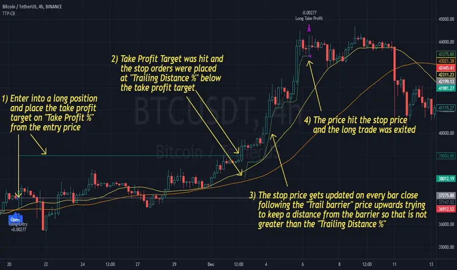
Trailing Take Profit - Close Based📝 Description
This script demonstrates a new approach to the trailing take profit.
Trailing Take Profit is a price-following technique. When used, instead of setting a limit order for the take profit target exiting from your position at the specified price, a stop order is conditionally set when the take profit target is reached. Then, the stop price (a.k.a trailing price), is placed below the take profit target at a distance defined by the user percentagewise. On regular time intervals, the stop price gets updated by following the "Trail Barrier" price (high by default) upwards. When the current price hits the stop price you exit the trade. Check the chart for more details.
This script demonstrates how to implement the close-based Trailing Take Profit logic for long positions, but it can also be applied for short positions if the logic is "reversed".
📢 NOTE
To generate some entries and showcase the "Trailing Take Profit" technique, this script uses the crossing of two moving averages. Please keep in mind that you should not relate the Backtesting results you see in the "Strategy Tester" tab with the success of the technique itself.
This is not a complete strategy per se, and the backtest results are affected by many parameters that are outside of the scope of this publication. If you choose to use this new approach of the "Trailing Take Profit" in your logic you have to make sure that you are backtesting the whole strategy.
⚔️ Comparison
In contrast to my older "Trailing Take Profit" publication where the trailing take profit implementation was tick-based, this new approach is close-based, meaning that the update of the stop price occurs at the bar close instead of every tick.
While comparing the real-time results of the two implementations is like comparing apples to oranges, because they have different dynamic behavior, the new approach offers better consistency between the backtesting results and the real-time results.
By updating the stop price on every bar close, you do not rely on the backtester assumptions anymore (check the Reasoning section below for more info).
The new approach resembles the conditional "Trailing Exit" technique, where the condition is true when the current price crosses over the take profit target. Then, the stop order is placed at the trailing price and it gets updated on every bar close to "follow" the barrier price (high). On the other hand, the older tick-based approach had more "tight" dynamics since the trailing price gets updated on every tick leaving less room for price fluctuations by making it more probable to reach the trailing price.
🤔 Reasoning
This new close-based approach addresses several practical issues the older tick-based approach had. Those issues arise mainly from the technicalities of the TV Backtester. More specifically, due to the assumptions the Broker Emulator makes for the price action of the history bars, the backtesting results in the TV Backtester are exaggerated, and depending on the timeframe, the backtesting results look way better than they are in reality.
The effect above, and the inability to reason about the performance of a strategy separated people into two groups. Those who never use this feature, because they couldn't know for sure the actual effect it might have in their strategy, (even if it turned out to be more profitable) and those who abused this type of "repainting" behavior to show off, and hijack some boosts from the community by boasting about the "fake" results of their strategies.
Even if there are ways to evaluate the effectiveness of the tick-based approach that is applied in an existing strategy (this is out of the topic of this publication), it requires extra effort to do the analysis. Using this closed-based approach we can have more predictable results, without surprises.
⚠️ Caveats
Since this approach updates the trailing price on bar close, you must wait for at least one bar to close after the price crosses over the take profit target.
Tillson T3 Moving Average - ScreenerScreener version of Tillson T3 Moving Average:
The T3 Moving Average generally produces entry signals similar to other moving averages and, thus, is mainly traded in the same manner. Here are several assumptions:
Suppose the price action is above the T3 Moving Average, and the indicator is upward. In that case, we have a bullish trend and should only enter long trades (advisable for novice/intermediate traders). If the price is below the T3 Moving Average and edging lower, we have a bearish trend and should limit entries to short.
About Screener Panel:
Users can explore 20 different and user-defined tickers, which can be changed from the SETTINGS (shares, crypto, commodities...) on this screener version.
The screener panel shows up right after the bars on the right side of the chart.
Tickers seen in green are the ones that are in an uptrend, according to T3.
The ones that appear in red are those in the SELL signal, in a downtrend.
The numbers in front of each Ticker indicate how many bars passed after the last BUY or SELL signal of T3.
For example, according to the indicator, when BTCUSDT appears (3) in GREEN, Bitcoin switched to a BUY signal 3 bars ago.
-In this screener version of Tillson T3 Moving Average, users can define the number of demanded tickers (symbols) from 1 to 20 by checking the relevant boxes on the settings tab.
-All selected tickers can be screened in different timeframes.
-Also, different timeframes of the same Ticker can be screened.
IMPORTANT NOTICE:
Screener shows the results in 2 different logic:
-Screener shows the information about the color changes of the T3 Moving Average with default settings.
-Users can check the "Change Screener to show T3 & Price Flips" button to activate the screener giving information about price flips.
If this option is preferred, users are advised to enlarge the length to have better signals.

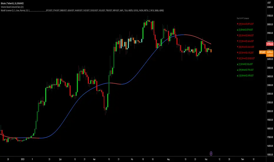
MavilimW ScreenerScreener version of MavilimW Moving Average :
Short-Term Examples (by decreasing 3 and 5 default values to have trading signals from color changes)
BUY when MavilimW turns blue from red.
SELL when MavW turns red from blue.
Long-Term Examples (with Default values 3 and 5)
BUY when the price crosses over the MavilimW line
SELL when the price crosses below the MavW line
MavilimW can also define significant SUPPORT and RESISTANCE levels in every period with its default values 3 and 5.
Screener Panel:
You can explore 20 different and user-defined tickers, which can be changed from the SETTINGS (shares, crypto, commodities...) on this screener version.
The screener panel shows up right after the bars on the right side of the chart.
Tickers seen in green are the ones that are in an uptrend, according to MavilimW.
The ones that appear in red are those in the SELL signal, in a downtrend.
The numbers in front of each Ticker indicate how many bars passed after the last BUY or SELL signal of MavW.
For example, according to the indicator, when BTCUSDT appears (3) in GREEN, Bitcoin switched to a BUY signal 3 bars ago.
-In this screener version of MavilimW, users can define the number of demanded tickers (symbols) from 1 to 20 by checking the relevant boxes on the settings tab.
-All selected tickers can be screened in different timeframes.
-Also, different timeframes of the same Ticker can be screened.
IMPORTANT NOTICE:
-Screener shows the information about the color changes of MavilimW Moving Average with default settings (as explained in the Short-Term Example section).
-Users can check the "Change Screener to show MavilimW & Price Flips" button to activate the screener as explained in the Short-Term Example section. Then the screener will give information about price flips.
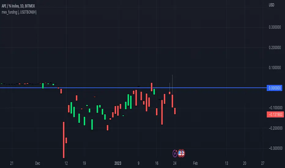
mex_fundingScript for calculating Bitmex funding based on the Premium tickers Bitmex submits to Tradingview
Make sure you add the correct Bitmex Interest Base and Quote Symbols in the input settings
For example for www.bitmex.com the inputs are:
Chart ticker: XBTUSDPI8H
Input Settings
Interest Base: XBTBON8H
Interest Quote: USDBON8H
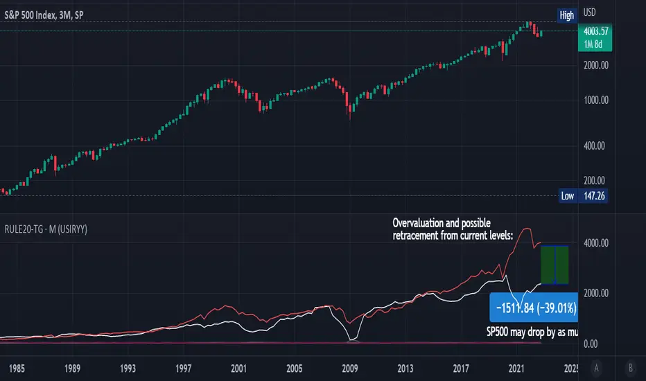
Rule Of 20 - Fair Value Estimation by Inflation & Earnings (TG)The Rule Of 20 is a heuristic calculation to find the fair value of an asset or market given its earnings and current inflation.
Its calculation is straightforward: the fair multiple of the price or price-to-earnings ratio of a stock should be 20 minus the rate of inflation.
In math terms: fair_price-to-earnings_ratio = (20 - inflation) ; fair_value = current_price * fair_price-to-earnings_ratio / real_price-to-earnings_ratio
For example, if a stock or index was trading on 11 times earnings and inflation was 2%, then the theory would be that the fair price-to-earnings ratio would be 20-2 = 18, which is much higher than the real price-to-earnings ratio of 11, and hence the asset would be undervalued.
Conversely, a market or company that was trading on 18 times price-to-earnings ration when inflation was 8% was seen as overvalued, because of the fair price-to-earnings ratio being 20-8=12, hence much lower than the real price-to-earnings ratio of 18.
We can then project the delta between the fair PE and real PE onto the asset's value to obtain the projected fair value, which may be a target of future value the asset may reach or hover around.
For example, as of 1st November 2022, SPX stood at 3871.97, with a PE ratio of 20.14 and an inflation in the US of 7.70. Using the Rule Of 20, we find that the fair PE ratio is 20-7.7=12.3, which is much lower than the current PE ratio of 20.14 by 39%! This may indicate a future possibility of a further downside risk by 39% from current valuation levels.
The origins of this rule are unknown, although the legendary US fund manager Peter Lynch is said to have been an active proponent when he was directing the Fidelity’s Magellan fund from 1977 to 1990.
For more infos about the Rule Of 20, reading this article is recommended: www.sharesmagazine.co.uk
This indicator implements the Rule Of 20 on any asset where the Financials are availble to TradingView, and also for the entire SP:SPX index as a way to assess the wider US stock market. Technically, the calculation is a bit different for the latter, as we cannot access earnings of SPX through Financials on TradingView, so we access it using the QUANDL:MULTPL/SP500_PE_RATIO_MONTH ticker instead.
By default are displayed:
current asset value in red
fair asset value according to the Rule Of 20 in white for SPX, or different shades of purple/maroon for other assets. Note that for SPX there is only one calculation, whereas for other assets there are multiple different ways to calculate earnings, so different fair values can be computed.
fair price-to-earnings ratio (PE ratio) in light grey.
real price-to-earnings ratio in darker grey.
This indicator can be used on SP:SPX ticker, and on most NASDAQ:* tickers, since they have Financials integrated in TradingView. Stocks tickers from other exchanges may not provide Financials data, so this indicator won't work then. If this happens, try to find the same ticker on NASDAQ instead.
Note that by default, only the US stock market is considered. If you want to consider stocks or assets in other regions of the world, please change the inflation ticker to a ticker that reflect the target region's inflation.
Also adding a table to ease interpretation was considered, but then the Timeframe MTF parameter would not work, and since the big advantage of this indicator is to allow for historical comparisons, the table was dropped.
Enjoy, and keep in mind that all models are wrong, but some are useful.
Trade safely!
TG
CVD - Cumulative Volume Delta Candles█ OVERVIEW
This indicator displays cumulative volume delta in candle form. It uses intrabar information to obtain more precise volume delta information than methods using only the chart's timeframe.
█ CONCEPTS
Bar polarity
By bar polarity , we mean the direction of a bar, which is determined by looking at the bar's close vs its open .
Intrabars
Intrabars are chart bars at a lower timeframe than the chart's. Each 1H chart bar of a 24x7 market will, for example, usually contain 60 bars at the lower timeframe of 1min, provided there was market activity during each minute of the hour. Mining information from intrabars can be useful in that it offers traders visibility on the activity inside a chart bar.
Lower timeframes (LTFs)
A lower timeframe is a timeframe that is smaller than the chart's timeframe. This script uses a LTF to access intrabars. The lower the LTF, the more intrabars are analyzed, but the less chart bars can display CVD information because there is a limit to the total number of intrabars that can be analyzed.
Volume delta
The volume delta concept divides a bar's volume in "up" and "down" volumes. The delta is calculated by subtracting down volume from up volume. Many calculation techniques exist to isolate up and down volume within a bar. The simplest techniques use the polarity of interbar price changes to assign their volume to up or down slots, e.g., On Balance Volume or the Klinger Oscillator . Others such as Chaikin Money Flow use assumptions based on a bar's OHLC values. The most precise calculation method uses tick data and assigns the volume of each tick to the up or down slot depending on whether the transaction occurs at the bid or ask price. While this technique is ideal, it requires huge amounts of data on historical bars, which usually limits the historical depth of charts and the number of symbols for which tick data is available.
This indicator uses intrabar analysis to achieve a compromise between the simplest and most precise methods of calculating volume delta. In the context where historical tick data is not yet available on TradingView, intrabar analysis is the most precise technique to calculate volume delta on historical bars on our charts. Our Volume Profile indicators use it. Other volume delta indicators in our Community Scripts such as the Realtime 5D Profile use realtime chart updates to achieve more precise volume delta calculations, but that method cannot be used on historical bars, so those indicators only work in real time.
This is the logic we use to assign intrabar volume to up or down slots:
• If the intrabar's open and close values are different, their relative position is used.
• If the intrabar's open and close values are the same, the difference between the intrabar's close and the previous intrabar's close is used.
• As a last resort, when there is no movement during an intrabar and it closes at the same price as the previous intrabar, the last known polarity is used.
Once all intrabars making up a chart bar have been analyzed and the up or down property of each intrabar's volume determined, the up volumes are added and the down volumes subtracted. The resulting value is volume delta for that chart bar.
█ FEATURES
CVD Candles
Cumulative Volume Delta Candles present volume delta information as it evolves during a period of time.
This is how each candle's levels are calculated:
• open : Each candle's' open level is the cumulative volume delta for the current period at the start of the bar.
This value becomes zero on the first candle following a CVD reset.
The candles after the first one always open where the previous candle closed.
The candle's high, low and close levels are then calculated by adding or subtracting a volume value to the open.
• high : The highest volume delta value found in intrabars. If it is not higher than the volume delta for the bar, then that candle will have no upper wick.
• low : The lowest volume delta value found in intrabars. If it is not lower than the volume delta for the bar, then that candle will have no lower wick.
• close : The aggregated volume delta for all intrabars. If volume delta is positive for the chart bar, then the candle's close will be higher than its open, and vice versa.
The candles are plotted in one of two configurable colors, depending on the polarity of volume delta for the bar.
CVD resets
The "cumulative" part of the indicator's name stems from the fact that calculations accumulate during a period of time. This allows you to analyze the progression of volume delta across manageable chunks, which is often more useful than looking at volume delta cumulated from the beginning of a chart's history.
You can configure the reset period using the "CVD Resets" input, which offers the following selections:
• None : Calculations do not reset.
• On a fixed higher timeframe : Calculations reset on the higher timeframe you select in the "Fixed higher timeframe" field.
• At a fixed time that you specify.
• At the beginning of the regular session .
• On a stepped higher timeframe : Calculations reset on a higher timeframe automatically stepped using the chart's timeframe and following these rules:
Chart TF HTF
< 1min 1H
< 3H 1D
<= 12H 1W
< 1W 1M
>= 1W 1Y
The indicator's background shows where resets occur.
Intrabar precision
The precision of calculations increases with the number of intrabars analyzed for each chart bar. It is controlled through the script's "Intrabar precision" input, which offers the following selections:
• Least precise, covering many chart bars
• Less precise, covering some chart bars
• More precise, covering less chart bars
• Most precise, 1min intrabars
As there is a limit to the number of intrabars that can be analyzed by a script, a tradeoff occurs between the number of intrabars analyzed per chart bar and the chart bars for which calculations are possible.
Total volume candles
You can choose to display candles showing the total intrabar volume for the chart bar. This provides you with more context to evaluate a bar's volume delta by showing it relative to the sum of intrabar volume. Note that because of the reasons explained in the "NOTES" section further down, the total volume is the sum of all intrabar volume rather than the volume of the bar at the chart's timeframe.
Total volume candles can be configured with their own up and down colors. You can also control the opacity of their bodies to make them more or less prominent. This publication's chart shows the indicator with total volume candles. They are turned off by default, so you will need to choose to display them in the script's inputs for them to plot.
Divergences
Divergences occur when the polarity of volume delta does not match that of the chart bar. You can identify divergences by coloring the CVD candles differently for them, or by coloring the indicator's background.
Information box
An information box in the lower-left corner of the indicator displays the HTF used for resets, the LTF used for intrabars, and the average quantity of intrabars per chart bar. You can hide the box using the script's inputs.
█ INTERPRETATION
The first thing to look at when analyzing CVD candles is the side of the zero line they are on, as this tells you if CVD is generally bullish or bearish. Next, one should consider the relative position of successive candles, just as you would with a price chart. Are successive candles trending up, down, or stagnating? Keep in mind that whatever trend you identify must be considered in the context of where it appears with regards to the zero line; an uptrend in a negative CVD (below the zero line) may not be as powerful as one taking place in positive CVD values, but it may also predate a movement into positive CVD territory. The same goes with stagnation; a trader in a long position will find stagnation in positive CVD territory less worrisome than stagnation under the zero line.
After consideration of the bigger picture, one can drill down into the details. Exactly what you are looking for in markets will, of course, depend on your trading methodology, but you may find it useful to:
• Evaluate volume delta for the bar in relation to price movement for that bar.
• Evaluate the proportion that volume delta represents of total volume.
• Notice divergences and if the chart's candle shape confirms a hesitation point, as a Doji would.
• Evaluate if the progress of CVD candles correlates with that of chart bars.
• Analyze the wicks. As with price candles, long wicks tend to indicate weakness.
Always keep in mind that unless you have chosen not to reset it, your CVD resets for each period, whether it is fixed or automatically stepped. Consequently, any trend from the preceding period must re-establish itself in the next.
█ NOTES
Know your volume
Traders using volume information should understand the volume data they are using: where it originates and what transactions it includes, as this can vary with instruments, sectors, exchanges, timeframes, and between historical and realtime bars. The information used to build a chart's bars and display volume comes from data providers (exchanges, brokers, etc.) who often maintain distinct feeds for intraday and end-of-day (EOD) timeframes. How volume data is assembled for the two feeds depends on how instruments are traded in that sector and/or the volume reporting policy for each feed. Instruments from crypto and forex markets, for example, will often display similar volume on both feeds. Stocks will often display variations because block trades or other types of trades may not be included in their intraday volume data. Futures will also typically display variations.
Note that as intraday vs EOD variations exist for historical bars on some instruments, differences may also exist between the realtime feeds used on intraday vs 1D or greater timeframes for those same assets. Realtime reporting rules will often be different from historical feed reporting rules, so variations between realtime feeds will often be different from the variations between historical feeds for the same instrument. The Volume X-ray indicator can help you analyze differences between intraday and EOD volumes for the instruments you trade.
If every unit of volume is both bought by a buyer and sold by a seller, how can volume delta make sense?
Traders who do not understand the mechanics of matching engines (the exchange software that matches orders from buyers and sellers) sometimes argue that the concept of volume delta is flawed, as every unit of volume is both bought and sold. While they are rigorously correct in stating that every unit of volume is both bought and sold, they overlook the fact that information can be mined by analyzing variations in the price of successive ticks, or in our case, intrabars.
Our calculations model the situation where, in fully automated order handling, market orders are generally matched to limit orders sitting in the order book. Buy market orders are matched to quotes at the ask level and sell market orders are matched to quotes at the bid level. As explained earlier, we use the same logic when comparing intrabar prices. While using intrabar analysis does not produce results as precise as when individual transactions — or ticks — are analyzed, results are much more precise than those of methods using only chart prices.
Not only does the concept underlying volume delta make sense, it provides a window on an oft-overlooked variable which, with price and time, is the only basic information representing market activity. Furthermore, because the calculation of volume delta also uses price and time variations, one could conceivably surmise that it can provide a more complete model than ones using price and time only. Whether or not volume delta can be useful in your trading practice, as usual, is for you to decide, as each trader's methodology is different.
For Pine Script™ coders
As our latest Polarity Divergences publication, this script uses the recently released request.security_lower_tf() Pine Script™ function discussed in this blog post . It works differently from the usual request.security() in that it can only be used at LTFs, and it returns an array containing one value per intrabar. This makes it much easier for programmers to access intrabar information.
Look first. Then leap.

Grid Bot AutoThis script is an auto-adjusting grid bot simulator. This is an improved version of the original Grid Bot Simulator. The grid bot is best used for ranging/choppy markets. Prices are divided into grids, or trade zones, that will trigger signals each time a new zone is entered. During ranging markets, each transaction is followed by a “take profit.” As the market starts to trend, transactions are stacked (compare to DCA ), until the market consolidates. No signals are triggered above the Upper Limit or Below the Lower Limit. Unlike the previous version, the upper and lower limits are calculated automatically. Grid levels are determined by four factors: Smoothing, Laziness, Elasticity, and Grid Intervals.
Smoothing:
A moving average (or linear regression) is applied to each close price as a basis. Options for smoothing are Linear Regression, Simple Moving Average, Exponential Moving Average, Volume-Weighted Moving Average, Triple-Exponential Moving Average.
Laziness:
Laziness is the percentage change required to reach the next level. If laziness is 1.5, the price must move up or down by 1.5% before the grid will change. This concept is based on Alex Grover’s Efficient Trend Step. This allows the grids to be based on even price levels, as opposed to jagged moving averages.
Elasticity:
Elasticity is the degree of “stickiness” to the current price trend. If the smoothing line remains above (or below) the current grid center without reverting but still not enough to reach the next grid level, the grid line will start to curve toward the next grid level. Elasticity is added to (or subtracted from) the gridline by a factor of minimum system ticks for the current pair. Elasticity of zero will keep the gridlines horizontal. If elasticity is too high, the grid will distort.
Grid Intervals:
Grid intervals are the percentage of space between each grid.
Laziness = 4%, Elasticity = 0. Price must move at least 4% before reaching the next level. With zero elasticity, gridlines are straight.
Laziness = 5%, Elasticity = 100. For each bar at a new grid level, the grid will start “curve” toward the next price level (up if price is greater than the middle grid, down if less than middle grid). Elasticity is calculated by the user-inputted “Elasticity” multiplied by the minimum tick for the current pair (ELSTX = syminfo.mintick * iELSTX)
Try experimenting with different combinations of the Smoothing Length, Smoothing Type, Laziness, Elasticity, and Grid Intervals to find the optimum settings for each chart. Lower-priced pairs (e.g. XRP/ADA/DODGE) will require lower Elasticity. Also note that different exchanges may have different minimum tick values. For example, minimum tick for BITMEX:XBTUSD and BYBIT:BTCUSD is .5, but BINANCE:BTCUSDT and COINBASE:BTCUSD is .01.
s3.tradingview.com
DODGEUSDT, 5min. Laziness: 4%, Elasticity 2.5
Number of Grids: 2. Laziness: 3.75%. Elasticity: 150. Grid Interval 2%.
Settings Overview
Smoothing Length : Smoothing period
Smoothing Type : Linear Regression, Simple Moving Average, Exponential Moving Average, Volume-Weighted Moving Average, Triple-Exponential Moving Average
Laziness : Percentage required for price to move until it reaches the next level. If price does not reach the next level (up or down), the grid will remain the same as previous grid (because it’s lazy).
Elasticity : Amount of curvature toward the next grid, based on the current price trend. As elasticity increases, gridlines will curve up or down by a factor of the number of ticks since the last grid change.
Grid Interval : Percent between grid levels.
Number of Grids : Number of grids to show.
Cooldown : Number of bars to wait to prevent consecutive signals.
Grid Line Transparency : Lower transparencies brighten the gridlines; higher transparencies dim the gridlines. To hide the gridlines completely, enter 100.
Fill Transparency: Lower transparencies brighten the fill box; higher transparencies dim the fill box. To hide the fill box completely, enter 100.
Signal Size : Make signal triangles large or small.
Reset Buy/Sell Index When Grids Change : When a new grid is formed, resetting the index may prevent false signals (experimental)
Use Highs/Lows for Signals : If enabled, signals are triggered as soon as the price touches the next zone. If disabled, signals are triggered after bar closes. Enable this for “Once Per Bar alerts. Disable for “Once Per Bar Close” alerts.
Show Min Tick : If checked, syminfo.mintick is displayed in upper-righthand corner. Useful for estimating Laziness.
Reverse Fill Colors : Default fill for fill boxes is green after buy and red after sell. Check this box to reverse.
Note: The Grid Bot Simulator scripts are experimental and works in progress. Please feel free to comment or contact me if you have suggestions/complaints.

Join data and union of 2 hystorical markets
How to create a union from two contiguous Tradingview tickers (series)
Francesco Marzolo March 18, 2021
Go to the older ticker of the two, for example CME: SP1! and open it on Tradingview.
On the graph thus created, add this script.
In the indicator settings select the same ticker as the chart in Symbol1
while in Symbol2 the ticker from which to retrieve the most recent data, for example: SPX500
The operation this script does is examine each bar of the two tickers, where there is a value for the second it holds this one, where it does not exist in second ticker it keeps the value of the first one. This new series is called Merge. So now in the chart there will be 4 series:
- that of the original chart without script
- the same series loaded via script (Symbol1)
- series 2 of "new" data (Symbol2)
- the Merge series that "prefers" the Symbol2 data if present, otherwise it shows Symbol1
So now you have to change the visibility of the 4 series to see the differences:
- turn off the visibility of the chart indicator
- turn off the Symbol1 series in the script properties (old data only)
- switch off the Symbol2 series as well (only new data)
- switch on the Merge series (new data if existing, old if not present in the new ticker)
Compare (RSI) MACDHere I've created an indicator which can be used together with my "Compare (RSI) Ticker 3x" Indicator.
It makes it much easier to see the movements between the "RSI Ticker 1" and "RSI Ticker 2/3".
- The white line is the "MACD" of Ticker 1, which is the difference between the "RSI Ticker 1" and "RSI Ticker 2/3".
- The purple line is the "Signal" line, an EMA of the "MACD". (Length is adjustable)
- The "0-line" is the "RSI Ticker 2/3" line, when Ticker 2 is chosen, this will be blue coloured, when Ticker 3 is chosen it will be red.
Because 2 MACD in 1 indicator is way too messy, you only can choose the comparison against Ticker 2 OR Ticker 3.
- In "Settings" > "Inputs" you can enable/disable the second or third Ticker
(If Ticker 2 is enabled, Ticker 3 is disabled and vice versa)
- The second Ticker has multiple choices
- The third you can type any Ticker you want, for example CRYPTOCAP:BNB, BINANCE:ETHUSDT, NASDAQ_DLY:NDX or whatever,
just start typing and you'll see the possibilities (You also can choose between "Cryptocurrencies", "Index", "Forex", ...)
- When the "MACD" crosses the "0-line", arrows will appear, white ones for "MACD", purple ones for the "Signal" line.
- The "Histogram" makes it easier to see the difference between "MACD" and "Signal" line.
- The source of this indicator is adjustable
- When the second chosen Ticker is the same as the first Ticker, of course you will be seeing lines
(because there is no difference between the 2 Tickers, the EMA is visible though)
If you use both "Compare (RSI) Ticker 3x" AND "Compare (RSI) MACD", of course be aware that you have the same Ticker 2 or 3 in each indicator!