Simple Harmonic Oscillator (SHO)The indicator is based on Akram El Sherbini's article "Time Cycle Oscillators" published in IFTA journal 2018 (pages 78-80) (www.ftaa.org.hk)
The SHO is a bounded oscillator for the simple harmonic index that calculates the period of the market’s cycle. The oscillator is used for short and intermediate terms and moves within a range of -100 to 100 percent. The SHO has overbought and oversold levels at +40 and -40, respectively. At extreme periods, the oscillator may reach the levels of +60 and -60. The zero level demonstrates an equilibrium between the periods of bulls and bears. The SHO oscillates between +40 and -40. The crossover at those levels creates buy and sell signals. In an uptrend, the SHO fluctuates between 0 and +40 where the bulls are controlling the market. On the contrary, the SHO fluctuates between 0 and -40 during downtrends where the bears control the market. Reaching the extreme level -60 in an uptrend is a sign of weakness. Mostly, the oscillator will retrace from its centerline rather than the upper boundary +40. On the other hand, reaching +60 in a downtrend is a sign of strength and the oscillator will not be able to reach its lower boundary -40.
Centerline Crossover Tactic
This tactic is tested during uptrends. The buy signals are generated when the WPO/SHI cross their centerlines to the upside. The sell signals are generated when the WPO/SHI cross down their centerlines. To define the uptrend in the system, stocks closing above their 50-day EMA are considered while the ADX is above 18.
Uptrend Tactic
During uptrends, the bulls control the markets, and the oscillators will move above their centerline with an increase in the period of cycles. The lower boundaries and equilibrium line crossovers generate buy signals, while crossing the upper boundaries will generate sell signals. The “Re-entry” and “Exit at weakness” tactics are combined with the uptrend tactic. Consequently, we will have three buy signals and two sell signals.
Sideways Tactic
During sideways, the oscillators fluctuate between their upper and lower boundaries. Crossing the lower boundary to the upside will generate a buy signal. On the other hand, crossing the upper boundary to the downside will generate a sell signal. When the bears take control, the oscillators will cross down the lower boundaries, triggering exit signals. Therefore, this tactic will consist of one buy signal and two sell signals. The sideway tactic is defined when stocks close above their 50-day EMA and the ADX is below 18
在腳本中搜尋"股价站上60月线"

Volume Profile [Makit0]VOLUME PROFILE INDICATOR v0.5 beta
Volume Profile is suitable for day and swing trading on stock and futures markets, is a volume based indicator that gives you 6 key values for each session: POC, VAH, VAL, profile HIGH, LOW and MID levels. This project was born on the idea of plotting the RTH sessions Value Areas for /ES in an automated way, but you can select between 3 different sessions: RTH, GLOBEX and FULL sessions.
Some basic concepts:
- Volume Profile calculates the total volume for the session at each price level and give us market generated information about what price and range of prices are the most traded (where the value is)
- Value Area (VA): range of prices where 70% of the session volume is traded
- Value Area High (VAH): highest price within VA
- Value Area Low (VAL): lowest price within VA
- Point of Control (POC): the most traded price of the session (with the most volume)
- Session HIGH, LOW and MID levels are also important
There are a huge amount of things to know of Market Profile and Auction Theory like types of days, types of openings, relationships between value areas and openings... for those interested Jim Dalton's work is the way to come
I'm in my 2nd trading year and my goal for this year is learning to daytrade the futures markets thru the lens of Market Profile
For info on Volume Profile: TV Volume Profile wiki page at www.tradingview.com
For info on Market Profile and Market Auction Theory: Jim Dalton's book Mind over markets (this is a MUST)
BE AWARE: this indicator is based on the current chart's time interval and it only plots on 1, 2, 3, 5, 10, 15 and 30 minutes charts.
This is the correlation table TV uses in the Volume Profile Session Volume indicator (from the wiki above)
Chart Indicator
1 - 5 1
6 - 15 5
16 - 30 10
31 - 60 15
61 - 120 30
121 - 1D 60
This indicator doesn't follow that correlation, it doesn't get the volume data from a lower timeframe, it gets the data from the current chart resolution.
FEATURES
- 6 key values for each session: POC (solid yellow), VAH (solid red), VAL (solid green), profile HIGH (dashed silver), LOW (dashed silver) and MID (dotted silver) levels
- 3 sessions to choose for: RTH, GLOBEX and FULL
- select the numbers of sessions to plot by adding 12 hours periods back in time
- show/hide POC
- show/hide VAH & VAL
- show/hide session HIGH, LOW & MID levels
- highlight the periods of time out of the session (silver)
- extend the plotted lines all the way to the right, be careful this can turn the chart unreadable if there are a lot of sessions and lines plotted
SETTINGS
- Session: select between RTH (8:30 to 15:15 CT), GLOBEX (17:00 to 8:30 CT) and FULL (17:00 to 15:15 CT) sessions. RTH by default
- Last 12 hour periods to show: select the deph of the study by adding periods, for example, 60 periods are 30 natural days and around 22 trading days. 1 period by default
- Show POC (Point of Control): show/hide POC line. true by default
- Show VA (Value Area High & Low): show/hide VAH & VAL lines. true by default
- Show Range (Session High, Low & Mid): show/hide session HIGH, LOW & MID lines. true by default
- Highlight out of session: show/hide a silver shadow over the non session periods. true by default
- Extension: Extend all the plotted lines to the right. false by default
HOW TO SETUP
BE AWARE THIS INDICATOR PLOTS ONLY IN THE FOLLOWING CHART RESOLUTIONS: 1, 2, 3, 5, 10, 15 AND 30 MINUTES CHARTS. YOU MUST SELECT ONE OF THIS RESOLUTIONS TO THE INDICATOR BE ABLE TO PLOT
- By default this indicator plots all the levels for the last RTH session within the last 12 hours, if there is no plot try to adjust the 12 hours periods until the seesion and the periods match
- For Globex/Full sessions just select what you want from the dropdown menu and adjust the periods to plot the values
- Show or hide the levels you want with the 3 groups: POC line, VA lines and Session Range lines
- The highlight and extension options are for a better visibility of the levels as POC or VAH/VAL
THANKS TO
@watsonexchange for all the help, ideas and insights on this and the last two indicators (Market Delta & Market Internals) I'm working on my way to a 'clean chart' but for me it's not an easy path
@PineCoders for all the amazing stuff they do and all the help and tools they provide, in special the Script-Stopwatch at that was key in lowering this indicator's execution time
All the TV and Pine community, open source and shared knowledge are indeed the best way to help each other
IF YOU REALLY LIKE THIS WORK, please send me a comment or a private message and TELL ME WHAT you trade, HOW you trade it and your FAVOURITE SETUP for pulling out money from the market in a consistent basis, I'm learning to trade (this is my 2nd year) and I need all the help I can get
GOOD LUCK AND HAPPY TRADING

lsi (study about length and MTF) Here in this example I took lazy bear famous momentum squeeze indicator . the problem that there is lagging in the indicator so the buy and sell will be late . So instead the KC length that the original script had we put
int1=input(30)
int2=input(60)
lengthKC=isintraday and interval >= int1 ? int2/interval * 7 : isintraday and interval < 60 ? 60/interval * 24 * 7 : 7
this allow us to create a time and length related function to indicator and result in better output with no lagging
The second and most important thing is the ability to create indicator with time function as MTF without the security function that create repaint
all you need to do is to change int2 (to the time min of your choice ) and you can create an indicator with MTF function without the security function .And by this hopefully avoid the repainting issue
when you use this indicator change the setting of int1 and int 2 according to time frame that you use
lets say 15 min graph
make the int1 <15 min and the int2 at 15 min. if you want to see it as MTF just increase the int2 to the time set of your choice and play little with int1 to best setting

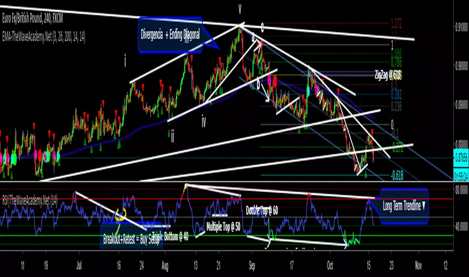
RSI with Visual Buy/Sell Setup | Corrective/Impulsive IndicatorRSI with Visual Buy/Sell Setup | 40-60 Support/Resistance | Corrective/Impulsive Indicator v2.15
|| RSI - The Complete Guide PDF ||
Modified Zones with Colors for easy recognition of Price Action.
Resistance @ downtrend = 60
Support @ uptrend = 40
Over 70 = Strong Bullish Impulse
Under 30 = Strong Bearish Impulse
Uptrend : 40-80
Downtrend: 60-20
--------------------
Higher Highs in price, Lower Highs in RSI = Bearish Divergence
Lower Lows in price, Higher Lows in RSI = Bullish Divergence
--------------------
Trendlines from Higher/Lower Peaks, breakout + retest for buy/sell setups.
###################
There are multiple ways for using RSI, not only divergences, but it confirms the trend, possible bounce for continuation and signals for possible trend reversal.
There's more advanced use of RSI inside the book RSI: The Complete Guide
Go with the force, and follow the trend.
"The Force is more your friend than the trend"
Build A Bot Hull TriggerThis is the automated trading system we built during the 60-Minute Build-A-Bot webinar on September 12, 2018. We had a lot of fun, and implemented a TON of indicators LIVE during this webinar! And the best part is that as a group we researched, designed, and built a profitable robot in exactly 60 minutes!
We started by voting on the type of trading system, and this is a trend following system because it got the most votes. Then, the attendees in the webinar sent in their suggestions for indicators and settings during the live webinar (still counting toward the 60 minutes). Once we had the indicators on the chart, and we discussed various settings we could use, we got to work building the robot, and ran the first strategy test...and it was profitable!
This version uses the Hull Moving Average as a trigger for initiating the trade, and everything else is the same for the filters. The other version uses the CCI as a trigger for the trade, and many other indicators as filters.

Indicators: Volume Zone Indicator & Price Zone IndicatorVolume Zone Indicator (VZO) and Price Zone Indicator (PZO) are by Waleed Aly Khalil.
Volume Zone Indicator (VZO)
------------------------------------------------------------
VZO is a leading volume oscillator that evaluates volume in relation to the direction of the net price change on each bar.
A value of 40 or above shows bullish accumulation. Low values (< 40) are bearish. Near zero or between +/- 20, the market is either in consolidation or near a break out. When VZO is near +/- 60, an end to the bull/bear run should be expected soon. If that run has been opposite to the long term price trend direction, then a reversal often will occur.
Traditional way of looking at this also works:
* +/- 40 levels are overbought / oversold
* +/- 60 levels are extreme overbought / oversold
More info:
drive.google.com
Price Zone Indicator (PZO)
------------------------------------------------------------
PZO is interpreted the same way as VZO (same formula with "close" substituted for "volume").
Chart Markings
------------------------------------------------------------
In the chart above,
* The red circles indicate a run-end (or reversal) zones (VZO +/- 60).
* Blue rectangle shows the consolidation zone (VZO betwen +/- 20)
I have been trying out VZO only for a week now, but I think this has lot of potential. Give it a try, let me know what you think.

FluxPulse Beacon## FluxPulse Beacon
FluxPulse Beacon applies a microstructure lens to every bar, combining directional thrust, realized volatility, and multi-timeframe liquidity checks to decide whether the tape is being pushed by real sponsorship or just noise. The oscillator's color-coded columns and adaptive burst thresholds transform complex flow dynamics into a single actionable flux score for futures and equities traders.
HOW IT WORKS
Momentum Extraction – Price differentials over a configurable pulse distance are smoothed using exponential moving averages to isolate directional thrust without reacting to single prints.
Volatility + Liquidity Normalization – The momentum stream is divided by realized volatility and multiplied by both local and higher-timeframe EMA volume ratios, ensuring pulses only appear when volatility and liquidity align.
Adaptive Thresholding – A volatility-derived standard deviation of flux is blended with the base threshold so bursts scale automatically between low-volatility and high-volatility market conditions.
Divergence Engine – Linear regression slopes compare price vs. flux to tag bullish/bearish divergences, highlighting stealth accumulation or distribution zones.
HOW TO USE IT
Continuation Entries : Go with the trend when histogram bars stay above the adaptive threshold, the signal line confirms, and trend bias agrees—this is where liquidity-backed follow-through lives.
Fade Plays : Watch for divergence alerts and shrinking compression values; when flux prints below zero yet price grinds higher, hidden selling pressure often precedes rollovers.
Session Filter : Compression percentage in the diagnostics table instantly tells you whether to trade thin overnight sessions—low compression means stand down.
VISUAL FEATURES
Dynamic background heat maps flux magnitude, while threshold lines provide a quick read on whether a pulse is statistically significant.
Diagnostics table displays live flux, signal, adaptive threshold, and compression for quick reference.
Alert-first workflow: The surface is intentionally clean—bursts and divergences are delivered via alerts instead of on-chart clutter.
PARAMETERS
Trend EMA Length (default: 34): Defines the macro bias anchor; increase for higher-timeframe confirmation.
Pulse Distance (default: 8): Controls how sensitive momentum extraction becomes.
Volatility Window (default: 21): Sample window for realized volatility normalization.
Liquidity Window (default: 55): Volume smoothing window that proxies liquidity expansion.
Liquidity Reference TF (default: 60): Select a higher timeframe to cross-check whether current volume matches institutional flows.
Adaptive Threshold (default: enabled): Disable for fixed thresholds on slower markets; enable for high-volatility assets.
Base Burst Threshold (default: 1.25): Minimum flux magnitude that qualifies as an actionable pulse.
ALERTS
The indicator includes four alert conditions:
Bull Burst: Detects upside liquidity pulses
Bear Burst: Detects downside liquidity pulses
Bull Divergence: Flags bullish delta divergence
Bear Divergence: Flags bearish delta divergence
LIMITATIONS
This indicator is designed for liquid futures and equity markets. Performance may degrade in low-volume or highly illiquid instruments. The adaptive threshold system works best on timeframes where sufficient volatility history exists (typically 15-minute charts and above). Divergence signals are probabilistic and should be confirmed with price action.
INSERT_CHART_SNAPSHOT_URL_HERE
---
## RangeLattice Mapper
RangeLattice Mapper constructs a higher-timeframe scaffolding on any intraday chart, locking in structural highs/lows, mid/quarter grids, VWAP confluence, and live acceptance/break analytics. It provides a non-repainting overlay that turns range management into a disciplined process.
HOW IT WORKS
Structure Harvesting – Using request.security() , the script samples highs/lows from a user-selected timeframe (default 240 minutes) over a configurable lookback to establish the dominant range.
Grid Construction – Midpoint and quarter levels are derived mathematically, mirroring how institutional traders map distribution/accumulation zones.
Acceptance Detection – Consecutive closes inside the range flip an acceptance flag and darken the cloud, signaling balanced auction conditions.
Break Confirmation – Multi-bar closes outside the structure raise break labels and alerts, filtering the countless fake-outs that plague breakout traders.
VWAP Fan Overlay – Session VWAP plus ATR-based bands provide a live measure of flow centering relative to the lattice.
HOW TO USE IT
Range Plays : Fade taps of the outer rails only when acceptance is active and VWAP sits inside the grid—this is where mean-reversion works best.
Breakout Plays : Wait for confirmed break labels before entering expansion trades; the dashboard's Width/ATR metric tells you if the expansion has enough fuel.
Market Prep : Carry the same lattice from pre-market into regular trading hours by keeping the structure timeframe fixed; alerts keep you notified even when managing multiple tickers.
VISUAL FEATURES
Range Tap and Mid Pivot markers provide a tape-reading breadcrumb trail for journaling.
Cloud fill opacity tightens when acceptance persists, visually signaling balance compressions ready to break.
Dashboard displays absolute width, ATR-normalized width, and current state (Balanced vs Transitional) so you can glance across charts quickly.
Acceptance Flag toggle: Keep the repeated acceptance squares hidden until you need to audit balance.
PARAMETERS
Structure Timeframe (default: 240): Choose the timeframe whose ranges matter most (4H for indices, Daily for stocks).
Structure Lookback (default: 60): Bars sampled on the structure timeframe.
Acceptance Bars (default: 8): How many consecutive bars inside the range confirm balance.
Break Confirmation Bars (default: 3): Bars required outside the range to validate a breakout.
ATR Reference (default: 14): ATR period for width normalization.
Show Midpoint Grid (default: enabled): Display the midpoint and quarter levels.
Show Adaptive VWAP Fan (default: enabled): Toggle the VWAP channel for assets where volume distribution matters most.
Show Acceptance Flags (default: disabled): Turn the acceptance markers on/off for maximum visual control.
Show Range Dashboard (default: enabled): Disable if screen space is limited, re-enable during prep sessions.
ALERTS
The indicator includes five alert conditions:
Range High Tap: Price interacted with the RangeLattice high
Range Low Tap: Price interacted with the RangeLattice low
Range Mid Tap: Price interacted with the RangeLattice mid
Range Break Up: Confirmed upside breakout
Range Break Down: Confirmed downside breakout
LIMITATIONS
This indicator works best on liquid instruments with clear structural levels. On very low timeframes (1-minute and below), the structure may update too frequently to be useful. The acceptance/break confirmation system requires patience—faster traders may find the multi-bar confirmation too slow for scalping. The VWAP fan is session-based and resets daily, which may not suit all trading styles.
---

SPX Breadth – Stocks Above 200-day SMA//@version=6
indicator("SPX Breadth – Stocks Above 200-day SMA",
overlay = false,
max_lines_count = 500,
max_labels_count = 500)
//–––––––––––––––––––––––––––––––––––––––––––––––––––––––––––––––––––––––––––––
// Inputs
group_source = "Source"
breadthSymbol = input.symbol("SPXA200R", "Breadth symbol", group = group_source)
breadthTf = input.timeframe("", "Timeframe (blank = chart)", group = group_source)
group_params = "Parameters"
totalStocks = input.int(500, "Total stocks in index", minval = 1, group = group_params)
smoothingLen = input.int(10, "SMA length", minval = 1, group = group_params)
//–––––––––––––––––––––––––––––––––––––––––––––––––––––––––––––––––––––––––––––
// Breadth series (symbol assumed to be percent 0–100)
string tf = breadthTf == "" ? timeframe.period : breadthTf
float rawPct = request.security(breadthSymbol, tf, close) // 0–100 %
float breadthN = rawPct / 100.0 * totalStocks // convert to count
float breadthSma = ta.sma(breadthN, smoothingLen)
//–––––––––––––––––––––––––––––––––––––––––––––––––––––––––––––––––––––––––––––
// Regime levels (0–20 %, 20–40 %, 40–60 %, 60–80 %, 80–100 %)
float lvl0 = 0.0
float lvl20 = totalStocks * 0.20
float lvl40 = totalStocks * 0.40
float lvl60 = totalStocks * 0.60
float lvl80 = totalStocks * 0.80
float lvl100 = totalStocks * 1.0
p0 = plot(lvl0, "0%", color = color.new(color.black, 100))
p20 = plot(lvl20, "20%", color = color.new(color.red, 0))
p40 = plot(lvl40, "40%", color = color.new(color.orange, 0))
p60 = plot(lvl60, "60%", color = color.new(color.yellow, 0))
p80 = plot(lvl80, "80%", color = color.new(color.green, 0))
p100 = plot(lvl100, "100%", color = color.new(color.green, 100))
// Colored zones
fill(p0, p20, color = color.new(color.maroon, 80)) // very oversold
fill(p20, p40, color = color.new(color.red, 80)) // oversold
fill(p40, p60, color = color.new(color.gold, 80)) // neutral
fill(p60, p80, color = color.new(color.green, 80)) // bullish
fill(p80, p100, color = color.new(color.teal, 80)) // very strong
//–––––––––––––––––––––––––––––––––––––––––––––––––––––––––––––––––––––––––––––
// Plots
plot(breadthN, "Stocks above 200-day", color = color.orange, linewidth = 2)
plot(breadthSma, "Breadth SMA", color = color.white, linewidth = 2)
// Optional label showing live value
var label infoLabel = na
if barstate.islast
label.delete(infoLabel)
string txt = "Breadth: " +
str.tostring(breadthN, format.mintick) + " / " +
str.tostring(totalStocks) + " (" +
str.tostring(rawPct, format.mintick) + "%)"
infoLabel := label.new(bar_index, breadthN, txt,
style = label.style_label_left,
color = color.new(color.white, 20),
textcolor = color.black)

Hybrid -WinCAlgo/// 🇬🇧
Hybrid - WinCAlgo is a weighted composite oscillator designed to provide a more robust and reliable signal than the standard Relative Strength Index (RSI). It integrates four different momentum and volume metrics—RSI, Money Flow Index (MFI), Scaled CCI, and VWAP-RSI—into a single 0-100 oscillator.
This powerful tool aims to filter market noise and enhance the detection of trend reversals by confirming momentum with trading volume and volume-weighted average price action.
⚪ What is this Indicator?
The Hybrid Oscillator combines:
* RSI (40% Weight): Measures fundamental price momentum.
* VWAP-RSI (40% Weight): Measures the momentum of the Volume Weighted Average Price (VWAP), providing strong volume confirmation for trend strength.
* MFI (10% Weight): Measures money flow volume, confirming momentum with liquidity.
* Scaled CCI (10% Weight): Tracks market extremes and potential trend shifts, scaled to fit the 0-100 range.
⚪ Key Features
* Composite Strength: Blends four different market factors for a multi-dimensional view of momentum.
* Volume Integration: High weights on VWAP-RSI and MFI ensure that momentum signals are backed by trading volume.
* Advanced Divergence: The robust formula significantly enhances the detection of Bullish and Bearish Divergences, often providing an earlier signal than traditional oscillators.
* Customizable: Adjustable Lookback Length (N) and Individual Component Weights allow users to fine-tune the oscillator for specific assets or timeframes.
* Visual Clarity: Uses 40/60 bands for earlier Overbought/Oversold indications, with a gradient-styled background for intuitive visual interpretation.
⚪ Usage
Use Hybrid – WinCAlgo as your primary momentum confirmation tool:
* Divergence Signals: Trust the indicator when it fails to confirm new price highs/lows; this signals imminent trend exhaustion and reversal.
* Accumulation/Distribution: Look for the oscillator to rise/fall while the price is ranging at a bottom/top; this confirms hidden buying or selling (accumulation).
* Overbought/Oversold: Use the 60 band as the trigger for potential selling/shorting signals, and the 40 band for potential buying/longing signals.
* Noise Filter: Combine with a higher timeframe chart (e.g., 4H or Daily) to filter out gürültü (noise) and focus only on significant momentum shifts.
---

Correlation Scanner📊 CORRELATION SCANNER - Financial Instruments Correlation Analyzer
🎯 ORIGINALITY AND PURPOSE
Correlation Scanner is a professional tool for analyzing correlation relationships between different financial instruments. Unlike standard correlation indicators that show the relationship between only two instruments, this script allows you to simultaneously track the correlation of up to 10 customizable instruments with a selected base asset.
The indicator is designed for traders working with cross-market analysis, portfolio diversification, and searching for related assets for arbitrage strategies.
🔧 HOW IT WORKS
The indicator uses the built-in ta.correlation() function to calculate the Pearson correlation coefficient between instrument closing prices over a specified period. Mathematical foundation:
1. Correlation Calculation: for each instrument, the correlation coefficient with the base asset is calculated over N bars (default 60)
2. Results Sorting: instruments are automatically ranked by absolute correlation value (from strongest to weakest)
3. Visualization: results are displayed in a table with color coding:
- Green: positive correlation (instruments move in the same direction)
- Red: negative correlation (instruments move in opposite directions)
- Color intensity depends on correlation strength
4. Correlation Strength Classification:
- Very Strong (💪💪💪): |r| > 0.8 — very strong relationship
- Strong (💪💪): |r| > 0.6 — strong relationship
- Medium (💪): |r| > 0.4 — medium relationship
- Weak: |r| > 0.2 — weak relationship
- Very Weak: |r| ≤ 0.2 — very weak relationship
📋 SETTINGS AND USAGE
MAIN PARAMETERS:
• Main Instrument — base instrument for comparison (default TVC:DXY - US Dollar Index)
• Correlation Period — calculation period in bars (10-500, default 60)
• Number of Instruments to Display — number of instruments to show (1-10)
• Table Position — table location on the chart
INSTRUMENT CONFIGURATION:
The indicator allows configuring up to 10 instruments for analysis. For each, you can specify:
• Instrument — instrument ticker (e.g., FX_IDC:EURUSD)
• Name — display name (emojis supported)
VISUAL SETTINGS:
• Show Chart Label with Correlation — display current chart's correlation with base instrument
• Table Header Color — table header color
• Table Row Background — table row background color
💡 USAGE EXAMPLES
1. DOLLAR IMPACT ANALYSIS: set DXY as the base instrument and track how dollar index changes affect currency pairs, gold, and cryptocurrencies
2. HEDGING ASSETS SEARCH: find instruments with strong negative correlation for risk diversification
3. PAIRS TRADING: identify assets with high positive correlation to find divergences and arbitrage opportunities
4. CROSS-MARKET ANALYSIS: track relationships between stocks, bonds, commodities, and currencies
5. SYSTEMIC RISK ASSESSMENT: identify periods of increased correlation between assets, which may indicate systemic risks
⚠️ IMPORTANT NOTES
• Correlation does NOT imply causation
• Correlation can change over time — regularly review the analysis period
• High past correlation doesn't guarantee the relationship will persist in the future
• Recommended to use the indicator in combination with fundamental analysis
🔔 ALERTS
The indicator includes a built-in alert condition: triggers when strong correlation (|r| > 0.8) is detected between the current chart and the base instrument.

CRT + SMC MY//@version=5
indicator("CRT + SMC MultiTF (Fixed Requests)", overlay=true, max_labels_count=500, max_boxes_count=200)
// ---------------- INPUTS ----------------
htfTF = input.string("60", title="HTF timeframe (60=1H, 240=4H)")
midTF = input.string("5", title="Mid timeframe (5 or 15)")
execTF = input.string("1", title="Exec timeframe (1 for sniper)")
useMAfilter = input.bool(true, "Require HTF MA filter")
htf_ma_len = input.int(50, "HTF MA length")
showOB = input.bool(true, "Show Order Blocks (midTF)")
showFVG = input.bool(true, "Show Fair Value Gaps (execTF)")
showEntries = input.bool(true, "Show Entry arrows & SL/TP")
slBuffer = input.int(3, "SL buffer (ticks)")
rrTarget = input.float(4.0, "Default R:R target")
useKillzone = input.bool(false, "Use London/NY Killzone (approx NY-5 timezone)")
// ---------------- REQUESTS (ALL at top-level) ----------------
// HTF series
htf_open = request.security(syminfo.tickerid, htfTF, open)
htf_high = request.security(syminfo.tickerid, htfTF, high)
htf_low = request.security(syminfo.tickerid, htfTF, low)
htf_close = request.security(syminfo.tickerid, htfTF, close)
htf_ma = request.security(syminfo.tickerid, htfTF, ta.sma(close, htf_ma_len))
htf_prev_high = request.security(syminfo.tickerid, htfTF, high )
htf_prev_low = request.security(syminfo.tickerid, htfTF, low )
// midTF series for OB detection
mid_open = request.security(syminfo.tickerid, midTF, open)
mid_high = request.security(syminfo.tickerid, midTF, high)
mid_low = request.security(syminfo.tickerid, midTF, low)
mid_close = request.security(syminfo.tickerid, midTF, close)
mid_median_body = request.security(syminfo.tickerid, midTF, ta.median(math.abs(close - open), 8))
// execTF series for FVG and micro structure
exec_high = request.security(syminfo.tickerid, execTF, high)
exec_low = request.security(syminfo.tickerid, execTF, low)
exec_open = request.security(syminfo.tickerid, execTF, open)
exec_close = request.security(syminfo.tickerid, execTF, close)
// Also get shifted values needed for heuristics (all top-level)
exec_high_1 = request.security(syminfo.tickerid, execTF, high )
exec_high_2 = request.security(syminfo.tickerid, execTF, high )
exec_low_1 = request.security(syminfo.tickerid, execTF, low )
exec_low_2 = request.security(syminfo.tickerid, execTF, low )
mid_low_1 = request.security(syminfo.tickerid, midTF, low )
mid_high_1 = request.security(syminfo.tickerid, midTF, high )
// ---------------- HTF logic ----------------
htf_ma_bias_long = htf_close > htf_ma
htf_ma_bias_short = htf_close < htf_ma
htf_sweep_high = (htf_high > htf_prev_high) and (htf_close < htf_prev_high)
htf_sweep_low = (htf_low < htf_prev_low) and (htf_close > htf_prev_low)
htf_final_long = htf_sweep_low and (not useMAfilter or htf_ma_bias_long)
htf_final_short = htf_sweep_high and (not useMAfilter or htf_ma_bias_short)
// HTF label (single label updated)
var label htf_label = na
if barstate.islast
label.delete(htf_label)
if htf_final_long
htf_label := label.new(bar_index, high, "HTF BIAS: LONG", style=label.style_label_left, color=color.green, textcolor=color.white)
else if htf_final_short
htf_label := label.new(bar_index, low, "HTF BIAS: SHORT", style=label.style_label_left, color=color.red, textcolor=color.white)
// ---------------- midTF OB detection (heuristic) ----------------
mid_body = math.abs(mid_close - mid_open)
is_bear_mid = (mid_open > mid_close) and (mid_body >= mid_median_body)
is_bull_mid = (mid_open < mid_close) and (mid_body >= mid_median_body)
mid_bear_disp = is_bear_mid and (mid_low < mid_low_1)
mid_bull_disp = is_bull_mid and (mid_high > mid_high_1)
// Store last OB values (safe top-level assignments)
var float last_bear_ob_top = na
var float last_bear_ob_bot = na
var int last_bear_ob_time = na
var float last_bull_ob_top = na
var float last_bull_ob_bot = na
var int last_bull_ob_time = na
if mid_bear_disp
last_bear_ob_top := mid_open
last_bear_ob_bot := mid_close
last_bear_ob_time := timenow
if mid_bull_disp
last_bull_ob_top := mid_close
last_bull_ob_bot := mid_open
last_bull_ob_time := timenow
// Draw OB boxes (draw always but can be toggled)
if showOB
if not na(last_bear_ob_top)
box.new(bar_index - 1, last_bear_ob_top, bar_index + 1, last_bear_ob_bot, border_color=color.new(color.red,0), bgcolor=color.new(color.red,85))
if not na(last_bull_ob_top)
box.new(bar_index - 1, last_bull_ob_top, bar_index + 1, last_bull_ob_bot, border_color=color.new(color.green,0), bgcolor=color.new(color.green,85))
// ---------------- execTF FVG detection (top-level logic) ----------------
// simple 3-candle gap heuristic
bull_fvg_local = exec_low_2 > exec_high_1
bear_fvg_local = exec_high_2 < exec_low_1
// Compute FVG box coords at top-level
fvg_bull_top = exec_high_1
fvg_bull_bot = exec_low_2
fvg_bear_top = exec_high_2
fvg_bear_bot = exec_low_1
if showFVG
if bull_fvg_local
box.new(bar_index - 2, fvg_bull_top, bar_index, fvg_bull_bot, border_color=color.new(color.green,0), bgcolor=color.new(color.green,85))
if bear_fvg_local
box.new(bar_index - 2, fvg_bear_top, bar_index, fvg_bear_bot, border_color=color.new(color.red,0), bgcolor=color.new(color.red,85))
// ---------------- micro structure on execTF ----------------
micro_high = exec_high
micro_low = exec_low
micro_high_1 = exec_high_1
micro_low_1 = exec_low_1
micro_bos_long = micro_high > micro_high_1
micro_bos_short = micro_low < micro_low_1
// ---------------- killzone check (top-level) ----------------
kill_ok = true
if useKillzone
hh = hour(time('GMT-5'))
mm = minute(time('GMT-5'))
// London approx
inLondon = (hh > 2 or (hh == 2 and mm >= 45)) and (hh < 5 or (hh == 5 and mm <= 0))
inNY = (hh > 8 or (hh == 8 and mm >= 20)) and (hh < 11 or (hh == 11 and mm <= 30))
kill_ok := inLondon or inNY
// ---------------- Entry logic (top-level boolean decisions) ----------------
hasBullOB = not na(last_bull_ob_top)
hasBearOB = not na(last_bear_ob_top)
entryLong = htf_final_long and hasBullOB and micro_bos_long and bull_fvg_local and kill_ok
entryShort = htf_final_short and hasBearOB and micro_bos_short and bear_fvg_local and kill_ok
// ---------------- SL / TP suggestions and plotting ----------------
var label lastEntryLabel = na
if entryLong or entryShort
entryPrice = close
suggestedSL = entryLong ? (htf_low - slBuffer * syminfo.mintick) : (htf_high + slBuffer * syminfo.mintick)
slDist = math.abs(entryPrice - suggestedSL)
suggestedTP = entryLong ? (entryPrice + slDist * rrTarget) : (entryPrice - slDist * rrTarget)
if showEntries
label.delete(lastEntryLabel)
lastEntryLabel := label.new(bar_index, entryPrice, entryLong ? "ENTRY LONG" : "ENTRY SHORT", style=label.style_label_center, color=entryLong ? color.green : color.red, textcolor=color.white)
line.new(bar_index, suggestedSL, bar_index + 20, suggestedSL, color=color.orange, style=line.style_dashed)
line.new(bar_index, suggestedTP, bar_index + 40, suggestedTP, color=color.aqua, style=line.style_dashed)
plotshape(entryLong, title="Entry Long", location=location.belowbar, color=color.green, style=shape.triangleup, size=size.small)
plotshape(entryShort, title="Entry Short", location=location.abovebar, color=color.red, style=shape.triangledown, size=size.small)
alertcondition(entryLong, title="CRT SMC Entry Long", message="Entry Long — HTF bias + midTF OB + execTF confirmation")
alertcondition(entryShort, title="CRT SMC Entry Short", message="Entry Short — HTF bias + midTF OB + execTF confirmation")

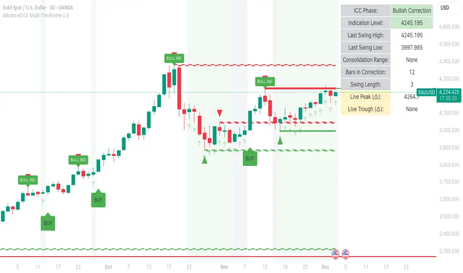
Advanced ICC Multi-Timeframe 1.0Advanced ICC Multi-Timeframe Trading System
A comprehensive implementation and interpretation of the Indication, Correction, Continuation (ICC) trading methodology made popular by Trades by Sci, enhanced with advanced multi-timeframe analysis and automation features.
⚠️ CRITICAL TRADING WARNINGS:
DO NOT blindly follow BUY/SELL signals from this indicator
This indicator shows potential entry points but YOU must validate each trade
PAPER TRADE EXTENSIVELY before risking real capital
BACKTEST THOROUGHLY on your chosen instruments and timeframes
The ICC methodology requires understanding and discretion - automated signals are guidance only
This tool aids analysis but does not replace proper trade planning, risk management, or trader judgment
⚠️ Important Disclaimers:
This indicator is not endorsed by or affiliated with Trades by Sci
This is an early implementation and interpretation of the ICC methodology
May not work exactly as Trades by Sci executes his trades and entries
Requires further debugging, backtesting, and real-world validation
Completely free to use - no purchase required
I'm just one person obsessed with this method and wanted some better visualization of the chart/entries
About ICC:
The ICC method identifies complete market cycles through three phases: Indication (breakout), Correction (pullback), and Continuation (entry). This indicator automates the identification of these phases and adds powerful features for modern traders.
Key Features:
Multi-Timeframe Capabilities:
Automatic timeframe detection with optimized settings for 5m, 15m, 30m, 1H, 4H, and Daily charts
Higher timeframe overlay to view HTF ICC levels on lower timeframe charts for precise entry timing
Smart defaults that adjust swing length and consolidation detection based on your timeframe
Advanced Phase Tracking:
Complete ICC cycle tracking: Indication, Correction, Consolidation, Continuation, and No Setup phases
Live structure detection shows potential peaks/troughs before full confirmation
Intelligent invalidation logic detects failed setups when market structure reverses
Dynamic phase backgrounds for instant visual confirmation
Three Types of Entry Signals:
Traditional Entries - Price crosses back through the original indication level (strongest signals)
"BUY" (green) / "SELL" (red)
Breakout Entries - Price breaks out of consolidation range in the same direction
"BUY" (green) / "SELL" (red)
Reversal Entries (Optional, can be toggled off) - Price breaks consolidation in opposite direction, indicating failed setup
"⚠ BUY" (yellow) / "⚠ SELL" (orange)
More aggressive, counter-trend signals
Can be disabled for more conservative trading
Professional Features:
Volatility-based support/resistance zones (ATR-adjusted) that adapt to market conditions
Historical zone tracking (0-3 configurable) with visual hierarchy
Comprehensive real-time info table displaying all key metrics
Full alert system for entries, indications, and consolidation detection
Visual distinction between high-confidence trend entries and cautionary reversal entries
📖 USAGE GUIDE
Entry Signal Types:
The indicator provides three types of entry signals with visual distinction:
Strong Entries (High Confidence):
"BUY" (bright green) / "SELL" (bright red)
Includes traditional entries (crossing back through indication level) and breakout entries (breaking consolidation in trend direction)
These are trend continuation or breakout signals with higher probability
Recommended for all traders
Reversal Entries (Caution - Counter-Trend):
"⚠ BUY" (yellow) / "⚠ SELL" (orange)
Triggered when price breaks out of correction/consolidation in the OPPOSITE direction
Indicates a failed setup and potential trend reversal
More aggressive, counter-trend plays
Can be toggled off in settings for more conservative trading
Recommended only for experienced traders or after thorough backtesting
Swing Length Settings:
The swing length determines how many bars on each side are needed to confirm a swing high/low. This is the most important setting for tuning the indicator to your style.
Auto Mode (Recommended for beginners): Toggle "Use Auto Timeframe Settings" ON
5-minute: 30 bars
15-minute: 20 bars
30-minute: 12 bars
1-hour: 7 bars
4-hour: 5 bars
Daily: 3 bars
Manual Mode: Toggle "Use Auto Timeframe Settings" OFF
Lower values (3-7): More aggressive, detects smaller swings
Pros: More signals, faster entries, catches smaller moves
Cons: More noise, more false signals, requires tighter stops
Best for: Scalping, active day trading, volatile markets
Higher values (12-20): More conservative, only major swings
Pros: More reliable signals, fewer false breakouts, clearer structure
Cons: Fewer signals, delayed entries, might miss smaller opportunities
Best for: Swing trading, position trading, trending markets
Default Manual Setting: 7 bars (balanced for 1H charts)
Minimum: 3 bars
Consolidation Bars Setting:
Determines how many bars without new structure are needed before flagging consolidation.
Lower values (3-10): Faster detection, catches brief pauses, more sensitive
Best for: Lower timeframes, volatile markets, avoiding any chop
Higher values (20-40): More reliable, only flags true extended consolidation
Best for: Higher timeframes, trending markets, patient traders
Current defaults scale with timeframe (more bars needed on shorter timeframes)
Historical S/R Zones:
Shows previous support and resistance levels to provide context.
Default: 2 historical zones (shows current + 2 previous)
Range: 0-3 zones
Visual Hierarchy: Older zones are more transparent with dashed borders
Usage: Higher numbers (2-3) show more historical context but can clutter the chart. Start with 2 and adjust based on your preference.
Live Structure Feature (Yellow Warning ⚠):
Provides early warning of potential structure changes before full confirmation.
What it does: Detects potential swing highs/lows after just 2 bars instead of waiting for full swing_length confirmation
Live Peak: Shows when a high is followed by 2 lower closes (potential top forming)
Live Trough: Shows when a low is followed by 2 higher closes (potential bottom forming)
Important: These are UNCONFIRMED - they may be invalidated if price reverses
Use case: Get early awareness of potential reversals while waiting for confirmation
Displayed in: Info table only (no visual markers on chart to reduce clutter)
Only shows: Peaks higher than last swing high, or troughs lower than last swing low (filters out noise)
Higher Timeframe (HTF) Analysis:
View higher timeframe ICC structure while trading on lower timeframes.
How to enable: Toggle "Show Higher Timeframe ICC" ON
Setup: Set "Higher Timeframe" to your reference timeframe
Example: Trading on 15-minute? Set HTF to 240 (4-hour) or 60 (1-hour)
Example: Trading on 5-minute? Set HTF to 60 (1-hour) or 15 (15-minute)
What it shows:
HTF indication levels displayed as dashed lines
Blue = HTF Bullish Indication
Purple = HTF Bearish Indication
HTF phase and levels shown in info table
Trading workflow:
Check HTF phase for overall market direction
Wait for HTF correction phase
Drop to lower timeframe to find precise entries
Enter when lower TF shows continuation in alignment with HTF
Best practice: HTF should be 3-4x your trading timeframe for best results
Reversal Entries Toggle:
Default: ON (shows all signal types)
Toggle OFF for more conservative trading (only trend continuation signals)
Recommended: Backtest with both settings to see which works better for your style
New traders should consider disabling reversal entries initially
Volatility-Based Zones:
When enabled, support/resistance zones automatically adjust their height based on ATR (Average True Range).
More volatile = wider zones
Less volatile = tighter zones
Toggle OFF for fixed-width zones
Community Feedback Welcome:
This is an evolving project and your input is valuable! Please share:
Bug reports and issues you encounter
Feature requests and suggestions for improvement
Results from your backtesting and live trading experience
Feedback on the reversal entry feature (too aggressive? working well?)
Ideas for better aligning with the ICC methodology
Perfect for traders learning or implementing the ICC methodology with the benefit of modern automation, multi-timeframe analysis, and flexible entry signal options.
Echo Chamber [theUltimator5]The Echo Chamber - When history repeats, maybe you should listen.
Ever had that eerie feeling you've seen this exact price action before? The Echo Chamber doesn't just give you déjà vu—it mathematically proves it, scales it, and projects what happened next.
📖 WHAT IT DOES
The Echo Chamber is an advanced pattern recognition tool that scans your chart's history to find segments that closely match your current price action. But here's where it gets interesting: it doesn't just find similar patterns - It expands and contracts the time window to create a uniquely scaled fractal. Patterns don't always follow the same timeframe, but they do follow similar patterns.
Using a custom correlation analysis algorithm combined with flexible time-scaling, this indicator:
Finds historical price segments that mirror your current market structure
Scales and overlays them perfectly onto your current chart
Projects forward what happened AFTER that historical match
Gives you a visual "echo" from the past with a glimpse into potential futures
══════════════════════════════
HOW TO USE IT
This indicator starts off in manual mode, which means that YOU, the user, can select the point in time that you want to project from. Simply click on a point in time to set the starting value.
Once you select your point in time, the indicator will automatically plot the chosen historical chart pattern and correlation over the current chart and project the price forwards based on how the chart looked in the past. If you want to change the point in time, you can update it from the settings, or drag the point on the chart over to a new position.
You can manually select any point in time, and the chart will quickly update with the new pattern. A correlation will be shown in a table alongside the date/timestamp of the selected point in time.
You can switch to auto mode, which will automatically search out the best-fit pattern over a defined lookback range and plot the past/future projection for you without having to manually select a point in time at all. It simply finds the best fit for you.
You can change the scale factor by adjusting multiplication and division variables to find time-scaled fractal patterns.
══════════════════════════════
🎯 KEY FEATURES
Two Operating Modes:
🔧 MANUAL MODE - Select any historical point and see how it correlates with current price action in real-time. Perfect for:
• Analyzing specific past events (crashes, rallies, consolidations)
• Testing historical patterns against current conditions
• Educational analysis of market structure repetition
🤖 AUTO MODE - It automatically scans through your lookback period to find the single best-correlated historical match. Ideal for:
• Quick pattern discovery
• Systematic trading approach
• Unbiased pattern recognition
Time Warp Technology:
The time warp feature expands and compresses the correlation window to provide a custom fractal so you can analyze windows of time that don't necessarily match the current chart.
💡 *Example: Multiplier=3, Divisor=2 gives you a 1.5x time stretch—perfect for finding patterns that played out 50% slower than current price action.*
Drawing Modes:
Scale Only : Pure vertical scaling—matches price range while maintaining temporal alignment at bar 0
Rotate & Scale : Advanced geometric transformation that anchors both the start AND end points, creating a rotated fit that matches your current segment's slope and range
Visual Components:
🟠 Orange Overlay : The historical match, perfectly scaled to your current price action
🟣 Purple Projection : What happened NEXT after that historical pattern (dotted line into the future)
📦 Highlight Boxes : Shows you exactly where in history these patterns came from
📊 Live Correlation Table : Real-time correlation coefficient with color-coded strength indicator
══════════════════════════════
⚙️ PARAMETERS EXPLAINED
Correlation Window Length (20) : How many bars to match. Smaller = more precise matches but noisier. Larger = broader patterns but fewer matches.
Note: if this value is too high in auto mode, the script may time out from computational overload.
Multiplication Factor : Historical time multiplier. 2 = sample every 2nd bar from history. Higher values find slower historical patterns.
Division Factor : Historical time divisor applied after multiplication. Final sample rate = (Length × Factor) ÷ Divisor, rounded down.
Lookback Range : How far back to search for patterns. More history = better chance of finding matches but slower performance.
Note: if this value is too high in auto mode, the script may time out from computational overload.
Future Projection Length : How many bars forward to project from the historical match. Your crystal ball's focal length.
══════════════════════════════
💼 TRADING APPLICATIONS
Trend Continuation/Reversal :
If the purple projection continues the current trend, that's your historical confirmation. If it reverses, you've found a potential turning point that's happened before under similar conditions.
Support/Resistance Validation :
Does the projection respect your S/R levels? History suggests those levels matter. Does it break through? You've found historical precedent for a breakout.
Time-Based Exits :
The projection shows not just WHERE price might go, but WHEN. Use it to anticipate timing of moves.
Multi-Timeframe Analysis :
Use time compression to overlay higher timeframe patterns onto lower timeframes. See daily patterns on hourly charts, weekly on daily, etc.
Pattern Education :
In Manual Mode, study how specific historical events correlate with current conditions. Build your pattern recognition library.
══════════════════════════════
📊 CORRELATION TABLE
The table shows your correlation coefficient as a percentage:
80-100%: Extremely strong correlation—history is practically repeating
60-80%: Strong correlation—significant similarity
40-60%: Moderate correlation—some structural similarity
20-40%: Weak correlation—limited similarity
0-20%: Very weak correlation—essentially random match
-20-40%: Weak inverse correlation
-40-60%: Moderate inverse correlation
-60-80%: Strong inverse correlation
-80-100%: Extremely strong inverse correlation—history is practically inverting
**Important**: The correlation measures SHAPE similarity, not price level. An 85% correlation means the price movements follow a very similar pattern, regardless of whether prices are higher or lower.
══════════════════════════════
⚠️ IMPORTANT DISCLAIMERS
- Past performance does NOT guarantee future results (but it sure is interesting to study)
- High correlation doesn't mean causation—markets are complex adaptive systems
- Use this as ONE tool in your analytical toolkit, not a standalone trading system
- The projection is what HAPPENED after a similar pattern in the past, not a prediction
- Always use proper risk management regardless of what the Echo Chamber suggests
══════════════════════════════
🎓 PRO TIPS
1. Start with Auto Mode to find high-correlation matches, then switch to Manual Mode to study why that period was similar
2. Experiment with time warping on different timeframes—a 2x factor on a daily chart lets you see weekly patterns
3. Watch for correlation decay —if correlation drops sharply after the match, current conditions are diverging from history
4. Combine with volume —check if volume patterns also match
5. Use "Rotate & Scale" mode when the current trend angle differs from the historical match
6. Increase lookback range to 500-1000+ on daily/weekly charts for finding rare historical parallels
══════════════════════════════
🔧 TECHNICAL NOTES
- Uses Pearson correlation coefficient for pattern matching
- Implements range-based scaling to normalize different price levels
- Rotation mode uses linear interpolation for geometric transformation
- All calculations are performed on close prices
- Boxes highlight actual historical bar ranges (high/low)
- Maximum of 500 lines and 500 boxes for performance optimization

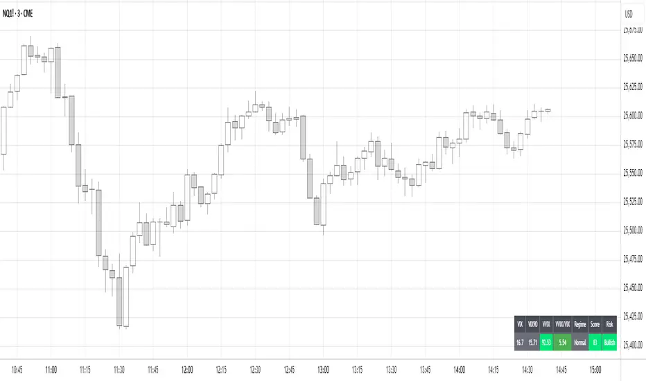
Volatility Regime NavigatorA guide to understanding VIX, VVIX, VIX9D, VVIX/VIX, and the Composite Risk Score
1. Purpose of the Indicator
This dashboard summarizes short-term market volatility conditions using four core volatility metrics.
It produces:
• Individual readings
• A combined Regime classification
• A Composite Risk Score (0–100)
• A simplified Risk Bucket (Bullish → Stress)
Use this to evaluate market fragility, drift potential, tail-risk, and overall risk-on/off conditions.
This is especially useful for intraday ES/NQ trading, expected-move context, and understanding when breakouts or fades have edge.
2. The Four Core Volatility Inputs
(1) VIX — Baseline Equity Volatility
• < 16: Complacent (easy drift-up, but watch for fragility)
• 16–22: Healthy, normal volatility → ideal trading conditions
• > 22: Stress rising
• > 26: Tail-risk / risk-off environment
(2) VIX9D — Short-Term Event Vol
Measures 9-day implied volatility. Reacts to immediate news/events.
• < 14: Strongly bullish (drift regime)
• 14–17: Bullish to neutral
• 17–20: Event risk building
• > 20: Short-term stress / caution
(3) VVIX — Volatility of VIX (fragility index)
Tracks volatility of volatility.
• < 100: “Bullish, Bullish” — very low fragility
• 100–120: Normal
• 120–140: Fragile
• > 140: Stress, hedging pressure
(4) VVIX/VIX Ratio — Microstructure Risk-On/Risk-Off
One of the most sensitive indicators of market confidence.
• 5.0–6.5: Strongest “normal/bullish” zone
• < 5.0: Bottom-stalking / fear regime
• > 6.5: Complacency → vulnerable to reversals
• > 7.5: Fragile / top-risk
3. Composite Risk Score (0–100)
The dashboard converts all four inputs into a single score.
Score Interpretation
• 80–100 → Bullish - Drift regime. Shallow pullbacks. Upside favored.
• 60–79 → Normal - Healthy tape. Balanced two-way trading.
• 40–59 → Fragile - Choppy, failed breakouts, thinner liquidity.
• 20–39 → Risk-Off - Downside tails active. Favor fades and defensive behavior.
• < 20 → Stress - Crisis or event-driven tape. Avoid longs.
Score updates every bar.
4. Regime Label
Independent of the composite score, the script provides a Regime classification based on combinations of VIX + VVIX/VIX:
• Bullish+ → Buying is easy, tape lifts passively
• Normal → Cleanest and most tradable conditions
• Complacent → Top-risk; be careful chasing upside
• Mixed → Signals conflict; chop potential
• Bottom Stalk → High VIX, low VVIX/VIX (capitulation signatures)
A trailing “+” or “*” indicates additional bullish or caution overlays from VIX9D/VVIX.
5. How to Use the Dashboard in Trading
When Bullish (Score ≥ 80):
• Expect drift-up behavior
• Downside limited unless catalyst hits
• Structure favors breakouts and trend continuation
• Mean reversion trades have lower expectancy
When Normal (Score 60–79):
• The “playbook regime”
• Breakouts and mean reversion both valid
• Best overall trading environment
When Fragile (Score 40–59):
• Expect chop
• Breakouts fail
• Take quicker profits
• Avoid overleveraged directional bets
When Risk-Off (20–39):
• Favor fades of strength
• Downside tails activate
• Trend-following short setups gain edge
• Respect volatility bands
When Stress (<20):
• Avoid long exposure
• Do not chase dips
• Expect violent, news-sensitive behavior
• Position sizing becomes critical
6. Quick Summary
• VIX = weather
• VIX9D = short-term storm radar
• VVIX = foundation stability
• VVIX/VIX = confidence vs fragility
• Composite Score = overall regime health
• Risk Bucket = simple “what do I do?” label
This dashboard gives traders a high-confidence, low-noise view of equity volatility conditions in real time.
Dual TF Bearish Divergence (Working)//@version=6
indicator("Dual TF Bearish Divergence (Working)", overlay=true)
// ----------------- SIMPLE BEARISH DIVERGENCE FUNCTION -------------------
bearDiv(src, rsiLen, lookbackMin, lookbackMax) =>
r = ta.rsi(src, rsiLen)
ph = ta.pivothigh(src, lookbackMin, lookbackMin)
ph_rsi = ta.pivothigh(r, lookbackMin, lookbackMin)
ph2 = ph
ph2_rsi = ph_rsi
priceHH = not na(ph) and not na(ph2) and ph > ph2
rsiLH = not na(ph_rsi) and not na(ph2_rsi) and ph_rsi < ph2_rsi
barsOk = lookbackMin >= lookbackMin and lookbackMin <= lookbackMax
priceHH and rsiLH and barsOk
// ----------------- TF CALLS -------------------
b60 = request.security(syminfo.tickerid, "60", bearDiv(close, 14, 10, 15))
b240 = request.security(syminfo.tickerid, "240", bearDiv(close, 14, 10, 15))
dual = b60 and b240
// ----------------- PLOT -------------------
plotshape(dual, title="Dual Bear Div", style=shape.labeldown,
color=color.red, size=size.small, text="🔻BearDiv")
// ----------------- ALERT -------------------
alertcondition(dual, "Dual Bearish Div 60+240",
"Bearish Divergence on both 60m & 240m")

Reversal_Detector//@version=6
indicator("상승 반전 탐지기 (Reversal Detector)", overlay=true)
// ==========================================
// 1. 설정 (Inputs)
// ==========================================
rsiLen = input.int(14, title="RSI 길이")
lbR = input.int(5, title="다이버전스 확인 범위 (오른쪽)")
lbL = input.int(5, title="다이버전스 확인 범위 (왼쪽)")
rangeUpper = input.int(60, title="RSI 과매수 기준")
rangeLower = input.int(30, title="RSI 과매도 기준")
// ==========================================
// 2. RSI 상승 다이버전스 계산 (핵심 로직)
// ==========================================
osc = ta.rsi(close, rsiLen)
// 피벗 로우(Pivot Low) 찾기: 주가의 저점
plFound = na(ta.pivotlow(osc, lbL, lbR)) ? false : true
// 다이버전스 조건 확인
// 1) 현재 RSI 저점이 이전 RSI 저점보다 높아야 함 (상승)
// 2) 현재 주가 저점이 이전 주가 저점보다 낮아야 함 (하락)
showBull = false
if plFound
// 이전 피벗 지점 찾기
oscLow = osc
priceLow = low
// 과거 데이터를 탐색하여 직전 저점과 비교
for i = 1 to 60
if not na(ta.pivotlow(osc, lbL, lbR) ) // 이전에 저점이 있었다면
prevOscLow = osc
prevPriceLow = low
// 다이버전스 조건: 가격은 더 떨어졌는데(Lower Low), RSI는 올랐을 때(Higher Low)
if priceLow < prevPriceLow and oscLow > prevOscLow and oscLow < rangeLower
showBull := true
break // 하나 찾으면 루프 종료
// ==========================================
// 3. 보조 조건 (MACD 골든크로스 & 이평선)
// ==========================================
= ta.macd(close, 12, 26, 9)
macdCross = ta.crossover(macdLine, signalLine) // MACD 골든크로스
ma5 = ta.sma(close, 5)
ma20 = ta.sma(close, 20)
maCross = ta.crossover(ma5, ma20) // 5일선이 20일선 돌파
// ==========================================
// 4. 시각화 (Plotting)
// ==========================================
// 1) 상승 다이버전스 발생 시 (강력한 바닥 신호)
plotshape(showBull,
title="상승 다이버전스",
style=shape.labelup,
location=location.belowbar,
color=color.red,
textcolor=color.white,
text="Bull Div\n(바닥신호)",
size=size.small,
offset=-lbR) // 과거 시점에 표시
// 2) MACD 골든크로스 (추세 확인용)
plotshape(macdCross and macdLine < 0, // 0선 아래에서 골든크로스 날 때만
title="MACD 골든크로스",
style=shape.triangleup,
location=location.belowbar,
color=color.yellow,
size=size.tiny,
text="MACD")
// 3) 이동평균선
plot(ma5, color=color.blue, title="5일선")
plot(ma20, color=color.orange, title="20일선")
// 알림 설정
alertcondition(showBull, title="상승 다이버전스 포착", message="상승 다이버전스 발생! 추세 반전 가능성")

Trend Trader//@version=6
indicator("Trend Trader", shorttitle="Trend Trader", overlay=true)
// User-defined input for moving averages
shortMA = input.int(10, minval=1, title="Short MA Period")
longMA = input.int(100, minval=1, title="Long MA Period")
// User-defined input for the instrument selection
instrument = input.string("US30", title="Select Instrument", options= )
// Set target values based on selected instrument
target_1 = instrument == "US30" ? 50 :
instrument == "NDX100" ? 25 :
instrument == "GER40" ? 25 :
instrument == "GOLD" ? 5 : 5 // default value
target_2 = instrument == "US30" ? 100 :
instrument == "NDX100" ? 50 :
instrument == "GER40" ? 50 :
instrument == "GOLD" ? 10 : 10 // default value
// User-defined input for the start and end times with default values
startTimeInput = input.int(12, title="Start Time for Session (UTC, in hours)", minval=0, maxval=23)
endTimeInput = input.int(17, title="End Time Session (UTC, in hours)", minval=0, maxval=23)
// Convert the input hours to minutes from midnight
startTime = startTimeInput * 60
endTime = endTimeInput * 60
// Function to convert the current exchange time to UTC time in minutes
toUTCTime(exchangeTime) =>
exchangeTimeInMinutes = exchangeTime / 60000
// Adjust for UTC time
utcTime = exchangeTimeInMinutes % 1440
utcTime
// Get the current time in UTC in minutes from midnight
utcTime = toUTCTime(time)
// Check if the current UTC time is within the allowed timeframe
isAllowedTime = (utcTime >= startTime and utcTime < endTime)
// Calculating moving averages
shortMAValue = ta.sma(close, shortMA)
longMAValue = ta.sma(close, longMA)
// Plotting the MAs
plot(shortMAValue, title="Short MA", color=color.blue)
plot(longMAValue, title="Long MA", color=color.red)
// MACD calculation for 15-minute chart
= request.security(syminfo.tickerid, "15", ta.macd(close, 12, 26, 9))
macdColor = macdLine > signalLine ? color.new(color.green, 70) : color.new(color.red, 70)
// Apply MACD color only during the allowed time range
bgcolor(isAllowedTime ? macdColor : na)
// Flags to track if a buy or sell signal has been triggered
var bool buyOnce = false
var bool sellOnce = false
// Tracking buy and sell entry prices
var float buyEntryPrice_1 = na
var float buyEntryPrice_2 = na
var float sellEntryPrice_1 = na
var float sellEntryPrice_2 = na
if not isAllowedTime
buyOnce :=false
sellOnce :=false
// Logic for Buy and Sell signals
buySignal = ta.crossover(shortMAValue, longMAValue) and isAllowedTime and macdLine > signalLine and not buyOnce
sellSignal = ta.crossunder(shortMAValue, longMAValue) and isAllowedTime and macdLine <= signalLine and not sellOnce
// Update last buy and sell signal values
if (buySignal)
buyEntryPrice_1 := close
buyEntryPrice_2 := close
buyOnce := true
if (sellSignal)
sellEntryPrice_1 := close
sellEntryPrice_2 := close
sellOnce := true
// Apply background color for entry candles
barcolor(buySignal or sellSignal ? color.yellow : na)
/// Creating buy and sell labels
if (buySignal)
label.new(bar_index, low, text="BUY", style=label.style_label_up, color=color.green, textcolor=color.white, yloc=yloc.belowbar)
if (sellSignal)
label.new(bar_index, high, text="SELL", style=label.style_label_down, color=color.red, textcolor=color.white, yloc=yloc.abovebar)
// Creating labels for 100-point movement
if (not na(buyEntryPrice_1) and close >= buyEntryPrice_1 + target_1)
label.new(bar_index, high, text=str.tostring(target_1), style=label.style_label_down, color=color.green, textcolor=color.white, yloc=yloc.abovebar)
buyEntryPrice_1 := na // Reset after label is created
if (not na(buyEntryPrice_2) and close >= buyEntryPrice_2 + target_2)
label.new(bar_index, high, text=str.tostring(target_2), style=label.style_label_down, color=color.green, textcolor=color.white, yloc=yloc.abovebar)
buyEntryPrice_2 := na // Reset after label is created
if (not na(sellEntryPrice_1) and close <= sellEntryPrice_1 - target_1)
label.new(bar_index, low, text=str.tostring(target_1), style=label.style_label_up, color=color.red, textcolor=color.white, yloc=yloc.belowbar)
sellEntryPrice_1 := na // Reset after label is created
if (not na(sellEntryPrice_2) and close <= sellEntryPrice_2 - target_2)
label.new(bar_index, low, text=str.tostring(target_2), style=label.style_label_up, color=color.red, textcolor=color.white, yloc=yloc.belowbar)
sellEntryPrice_2 := na // Reset after label is created

Smart MACD Divergence ScannerOriginal Base Indicator: "CM_MacD_Ult_MTF" by ChrisMoody
This indicator builds upon ChrisMoody's excellent multi-timeframe MACD foundation and transforms it into a professional divergence scanner with advanced quality assessment and filtering capabilities. The original MACD visualization and MTF functionality have been preserved while adding completely new divergence detection, scoring, and filtering systems.
🎯 What Makes This Indicator Unique:
Smart MACD Divergence Scanner is a professional tool for detecting MACD-based divergences with an advanced filtering system and signal quality assessment. Unlike standard divergence indicators, this version includes innovative features:
Adaptive Quality Scoring System — each signal receives a score from 0 to 100 based on multiple factors
Volatility Filter — automatic signal suppression during low market volatility periods
Multi-Timeframe Confirmation — divergence verification on higher timeframe for increased reliability
Divergence Strength Analysis — calculation of percentage difference between price and indicator movement
Information Dashboard — detailed real-time signal statistics
Cooldown System — prevention of multiple consecutive signals
💡 How It Works:
The indicator uses the classic divergence concept — the divergence between price movement and the MACD oscillator. However, instead of simple pivot detection, the algorithm:
Scans the market for local extremes (pivots) on price and MACD histogram
Searches for divergences — when price updates low/high while MACD shows opposite movement
Assesses quality — analyzes divergence strength, volatility, higher timeframe confirmation
Filters noise — eliminates weak signals through threshold system and cooldown
Generates signal — only when all quality criteria are met
🔧 Key Parameters:
MACD Settings: Fast Length (12), Slow Length (26), Signal Length (9)
Divergence Detection: Pivot Lookback (5), Max Lookback Range (60), Min Divergence Strength (15%)
Quality Filters: Min Quality Score (60), Volatility Filter, MTF Confirmation, Signal Cooldown (5)
📊 How to Use:
Add indicator to chart — it will automatically start scanning
Configure filters — start with default settings, then adapt to your trading style
Watch for signals: 🟢 Green "BUY" label = bullish divergence, 🔴 Red "SELL" label = bearish divergence
Check quality score on labels (Q: XX)
Use information panel to monitor statistics and current market conditions
⚙️ Settings Guide:
For swing trading (4H-Daily): Increase Pivot Lookback to 7-10, set Min Quality Score to 70+
For day trading (15m-1H): Keep default settings, enable all filters
For scalping (1m-5m): Decrease Min Quality Score to 50, disable MTF Confirmation
For volatile markets (crypto): Increase Min Divergence Strength to 20-25%, enable Volatility Filter
⚠️ Important Notes:
Divergences are probabilistic signals, not guaranteed reversals
Use additional confirmation (support/resistance levels, volume, price action)
Adjust parameters for specific asset and timeframe
Signals appear with Pivot Lookback bars delay (retrospective confirmation)
On volatile markets, increase Min Quality Score to reduce false signals

GRA v5 SNIPER# GRA v5 SNIPER - Documentation & Cheatsheet
## 🎯 Get Rich Aggressively v5 - SNIPER Edition
**Precision Futures Scalping | NQ • ES • YM • GC • BTC**
> **Philosophy:** *Quality over quantity. One sniper shot beats ten spray-and-pray attempts.*
---
## ⚡ QUICK CHEATSHEET
```
┌─────────────────────────────────────────────────────────────────────────────┐
│ GRA v5 SNIPER - QUICK REFERENCE │
├─────────────────────────────────────────────────────────────────────────────┤
│ │
│ 🎯 SIGNAL REQUIREMENTS (ALL MUST BE TRUE): │
│ ═══════════════════════════════════════════ │
│ ✓ Tier → B minimum (20+ pts NQ) │
│ ✓ Volume → 1.5x+ average │
│ ✓ Delta → 60%+ dominance (buyers OR sellers) │
│ ✓ Body → 70%+ of candle range │
│ ✓ Range → 1.3x+ average candle size │
│ ✓ Wicks → Small opposite wick (<50% of body) │
│ ✓ CVD → Trending with signal direction │
│ ✓ Session → London (3-5am ET) OR NY (9:30-11:30am ET) │
│ │
├─────────────────────────────────────────────────────────────────────────────┤
│ │
│ 📊 TIER ACTIONS: │
│ ════════════════ │
│ S-TIER (100+ pts) → 🥇 HOLD position, ride the wave │
│ A-TIER (50-99 pts) → 🥈 SWING for 2-3 minutes │
│ B-TIER (20-49 pts) → 🥉 SCALP quick, 30-60 seconds │
│ │
├─────────────────────────────────────────────────────────────────────────────┤
│ │
│ 🚨 ENTRY CHECKLIST: │
│ ═══════════════════ │
│ □ Signal appears (S🎯, A🎯, or B🎯) │
│ □ Table shows: Vol GREEN, Delta colored, Body GREEN │
│ □ CVD arrow matches direction (▲ for long, ▼ for short) │
│ □ Session active (LDN! or NY! in yellow) │
│ □ Enter at close of signal candle │
│ │
├─────────────────────────────────────────────────────────────────────────────┤
│ │
│ ⛔ DO NOT TRADE WHEN: │
│ ════════════════════ │
│ ✗ Session shows "---" (outside key hours) │
│ ✗ Vol shows RED (below 1.5x) │
│ ✗ Body shows RED (weak candle structure) │
│ ✗ Delta below 60% (no clear dominance) │
│ ✗ Multiple conflicting signals │
│ │
├─────────────────────────────────────────────────────────────────────────────┤
│ │
│ 📈 INSTRUMENT SETTINGS: │
│ ════════════════════════ │
│ NQ/ES (1-3 min): S=100, A=50, B=20 pts │
│ YM (1-5 min): S=100, A=50, B=25 pts │
│ GC (5-15 min): S=15, A=8, B=4 pts │
│ BTC (1-15 min): S=500, A=250, B=100 pts │
│ │
└─────────────────────────────────────────────────────────────────────────────┘
```
---
## 📋 DETAILED DOCUMENTATION
### What Makes SNIPER Different?
The SNIPER edition eliminates 80%+ of signals compared to standard GRA. Every signal that passes through has been validated by **8 independent filters**:
| Filter | Standard GRA | SNIPER GRA | Why It Matters |
|--------|-------------|------------|----------------|
| Volume | 1.3x avg | **1.5x avg** | Institutional participation |
| Delta | 55% | **60%** | Clear buyer/seller control |
| Body Ratio | None | **70%+** | No dojis or spinners |
| Range | None | **1.3x avg** | Significant price movement |
| Wicks | None | **<50% body** | Conviction in direction |
| CVD | None | **Required** | Trend confirmation |
| B-Tier Min | 10 pts | **20 pts** | Filter noise |
| Session | Optional | **Required** | Institutional hours |
---
### Signal Anatomy
When you see a signal like `A🎯`, here's what passed validation:
```
Signal: A🎯 LONG at 21,450.00
Validation Breakdown:
├── Points: 67.5 pts ✓ (A-Tier = 50-99)
├── Volume: 2.1x avg ✓ (≥1.5x required)
├── Delta: 68% Buyers ✓ (≥60% required)
├── Body: 78% of range ✓ (≥70% required)
├── Range: 1.6x avg ✓ (≥1.3x required)
├── Wick: Upper 15% ✓ (<50% of body)
├── CVD: ▲ Rising ✓ (Matches LONG)
└── Session: NY! ✓ (Active session)
RESULT: VALID SNIPER SIGNAL
```
---
### Table Legend
| Field | Reading | Color Meaning |
|-------|---------|---------------|
| **Pts** | Point movement | Gold/Green/Yellow = Tiered |
| **Tier** | S/A/B/X | Gold/Green/Yellow/White |
| **Vol** | Volume ratio | 🟢 ≥1.5x, 🔴 <1.5x |
| **Delta** | Buy/Sell % | 🟢 Buy dom, 🔴 Sell dom, ⚪ Neutral |
| **Body** | Body % of range | 🟢 ≥70%, 🔴 <70% |
| **CVD** | Cumulative delta | ▲ Bullish trend, ▼ Bearish trend |
| **Sess** | Session status | 🟡 Active, ⚫ Inactive |
---
### Trading Rules
#### Entry Rules
1. **Wait for signal** - Don't anticipate
2. **Verify table** - All conditions GREEN
3. **Enter at candle close** - Not during formation
4. **Position size by tier:**
- S-Tier: Full size
- A-Tier: 75% size
- B-Tier: 50% size
#### Exit Rules
| Tier | Target | Max Hold Time |
|------|--------|---------------|
| S | Let it run | 5-10 minutes |
| A | 1:1.5 R:R | 2-3 minutes |
| B | 1:1 R:R | 30-60 seconds |
#### Stop Loss
- Place at **opposite end of signal candle**
- For S-Tier: Allow 50% retracement
- For B-Tier: Tight stop, quick exit
---
### Session Priority
```
LONDON OPEN (3:00-5:00 AM ET)
════════════════════════════
• Best for: GC, European indices
• Characteristics: Stop hunts, reversals
• Look for: Sweeps of Asian session levels
NY OPEN (9:30-11:30 AM ET)
════════════════════════════
• Best for: NQ, ES, YM
• Characteristics: High volume, trends
• Look for: Continuation after 10 AM
```
---
### Common Mistakes to Avoid
| Mistake | Why It's Bad | Solution |
|---------|-------------|----------|
| Trading outside sessions | Low volume = fake moves | Wait for LDN! or NY! |
| Ignoring weak body | Dojis reverse | Body must be 70%+ |
| Fighting CVD | Swimming upstream | CVD must confirm |
| Oversizing B-Tier | Small moves = small size | 50% max on B |
| Chasing missed signals | FOMO loses money | Wait for next setup |
---
### Alert Setup
Configure these alerts in TradingView:
| Alert | Priority | Action |
|-------|----------|--------|
| 🎯 S-TIER LONG/SHORT | 🔴 High | Drop everything, check chart |
| 🎯 A-TIER LONG/SHORT | 🟠 Medium | Evaluate within 30 seconds |
| 🎯 B-TIER LONG/SHORT | 🟢 Low | Quick glance if available |
| LONDON/NY OPEN | 🔵 Info | Prepare for action |
---
### Pine Script v6 Notes
This indicator uses Pine Script v6 features:
- `request.security_lower_tf()` for intrabar delta
- Type inference for cleaner code
- Array operations for CVD calculation
**Minimum TradingView Plan:** Pro (for intrabar data)
---
## 🏆 Golden Rule
> **"If you have to convince yourself it's a good signal, it's not a good signal."**
The SNIPER edition is designed so that when a signal appears, there's nothing to think about. If all conditions are met, you trade. If any condition fails, you wait.
**Leave every trade with money. That's the goal.**
---
*© Alexandro Disla - Get Rich Aggressively v5 SNIPER*
*Pine Script v6 | TradingView*

Sideways & Breakout Detector + Forecast//@version=6
indicator("Sideways & Breakout Detector + Forecast", overlay=true, max_labels_count=500)
// Inputs
lengthATR = input.int(20, "ATR Länge")
lengthMA = input.int(50, "Trend MA Länge")
sqFactor = input.float(1.2, "Seitwärtsfaktor")
brkFactor = input.float(1.5, "Breakoutfaktor")
// ATR / Volatilität
atr = ta.atr(lengthATR)
atrSMA = ta.sma(atr, lengthATR)
// Basislinie / Trend
basis = ta.sma(close, lengthATR)
trendMA = ta.sma(close, lengthMA)
// Seitwärtsbedingung
isSideways = atr < atrSMA * sqFactor
// Breakouts
upperBreak = close > basis + atr * brkFactor
lowerBreak = close < basis - atr * brkFactor
// Vorhergesagter Ausbruch (Forecast)
// Wenn Seitwärtsphase + Kurs nahe obere oder untere Kanalgrenze
forecastBull = isSideways and (close > basis + 0.5 * atr)
forecastBear = isSideways and (close < basis - 0.5 * atr)
// Farben
barcolor(isSideways ? color.new(color.yellow, 40) : na)
barcolor(upperBreak ? color.green : na)
barcolor(lowerBreak ? color.red : na)
// Breakout-Bänder
plot(basis + atr * brkFactor, "Bull Break Zone", color=color.new(color.green, 60))
plot(basis - atr * brkFactor, "Bear Break Zone", color=color.new(color.red, 60))
// Labels (klein)
if isSideways
label.new(bar_index, close, "Seitwärts", color=color.yellow, style=label.style_label_center, size=size.tiny)
if upperBreak
label.new(bar_index, high, "Bull Breakout", color=color.green, style=label.style_label_up, size=size.tiny)
if lowerBreak
label.new(bar_index, low, "Bear Breakout", color=color.red, style=label.style_label_down, size=size.tiny)
// Vorhergesagte Ausbrüche markieren
plotshape(forecastBull, title="Forecast Bull", location=location.abovebar, color=color.new(color.green, 0), style=shape.triangleup, size=size.tiny)
plotshape(forecastBear, title="Forecast Bear", location=location.belowbar, color=color.new(color.red, 0), style=shape.triangledown, size=size.tiny)
// Alerts
alertcondition(isSideways, "Seitwärtsphase", "Der Markt läuft seitwärts.")
alertcondition(upperBreak, "Bull Breakout", "Ausbruch nach oben!")
alertcondition(lowerBreak, "Bear Breakout", "Ausbruch nach unten!")
alertcondition(forecastBull, "Forecast Bull", "Voraussichtlicher Bull-Ausbruch!")
alertcondition(forecastBear, "Forecast Bear", "Voraussichtlicher Bear-Ausbruch!")

Stratégie SMC V18.2 (BTC/EUR FINAL R3 - Tendance)This strategy is an automated implementation of Smart Money Concepts (SMC), designed to operate on the Bitcoin/Euro (BTC/EUR) chart using the 15-minute Timeframe (M15).It focuses on identifying high-probability zones (Order Blocks) after a confirmed Break of Structure (BOS) and a Liquidity Sweep, utilizing an H1/EMA 200 trend filter to only execute trades in the direction of the dominant market flow.Risk management is strict: every trade uses a fixed Risk-to-Reward Ratio (R:R) of 1:3.🧱 Core Logic Components
1. Trend Filter (H1/EMA 200)Objective: To avoid counter-trend entries, which has allowed the success rate to increase to nearly $65\%$ in backtests.Mechanism: A $200$-period EMA is plotted on a higher timeframe (Default: H1/60 minutes).Long (Buy): Entry is only permitted if the current price (M15) is above the trend EMA.Short (Sell): Entry is only permitted if the current price (M15) is below the trend EMA.
2. Order Block (OB) DetectionA potential Order Block is identified on the previous candle if it is
accompanied by an inefficiency (FVG - Fair Value Gap).
3. Advanced SMC ValidationBOS (Break of Structure): A recent BOS must be confirmed by breaking the swing high/low defined by the swing length (Default: 4 M15 candles).Liquidity (Liquidity Sweep): The Order Block zone must have swept recent liquidity (defined by the Liquidity Search Length) within a certain tolerance (Default: $0.1\%$).Point of Interest: The OB must form in a premium zone (for shorts) or a discount zone (for longs) relative to the current swing range (above or below the $50\%$ level of the range).
4. Execution and Risk ManagementEntry: The trade is triggered when the price touches the active Order Block (mitigation).Stop Loss (SL): The SL is fixed at the low of the OB (for longs) or the high of the OB (for shorts).Take Profit (TP): The TP is strictly set at a level corresponding to 3 times the SL distance (R:R 1:3).Lot Sizing: The trade quantity is calculated to risk a fixed amount (Default: 2.00 Euros) per transaction, capped by a Lot Max and Lot Min defined by the user.
Input Parameters (Optimized for BTC/EUR M15)Users can adjust these parameters to modify sensitivity and risk profile. The default values are those optimized for the high-performing backtest (Profit Factor $> 3$).ParameterDescriptionDefault Value (M15)Long. Swing (BOS)Candle length used to define the swing (and thus the BOS).4Long. Recherche Liq.Number of candles to scan to confirm a liquidity sweep.7Tolérance Liq. (%)Price tolerance to validate the liquidity sweep (as a percentage of price).0.1Timeframe TendanceChart timeframe used for the EMA filter (e.g., 60 = H1).60 (H1)Longueur EMA TendancePeriods used for the trend EMA.200Lot Max (Quantité Max BTC)Maximum quantity of BTC the strategy is allowed to trade.0.01Lot Min Réel (Exigence Broker)Minimum quantity required by the broker/exchange.0.00001

Dimensional Resonance ProtocolDimensional Resonance Protocol
🌀 CORE INNOVATION: PHASE SPACE RECONSTRUCTION & EMERGENCE DETECTION
The Dimensional Resonance Protocol represents a paradigm shift from traditional technical analysis to complexity science. Rather than measuring price levels or indicator crossovers, DRP reconstructs the hidden attractor governing market dynamics using Takens' embedding theorem, then detects emergence —the rare moments when multiple dimensions of market behavior spontaneously synchronize into coherent, predictable states.
The Complexity Hypothesis:
Markets are not simple oscillators or random walks—they are complex adaptive systems existing in high-dimensional phase space. Traditional indicators see only shadows (one-dimensional projections) of this higher-dimensional reality. DRP reconstructs the full phase space using time-delay embedding, revealing the true structure of market dynamics.
Takens' Embedding Theorem (1981):
A profound mathematical result from dynamical systems theory: Given a time series from a complex system, we can reconstruct its full phase space by creating delayed copies of the observation.
Mathematical Foundation:
From single observable x(t), create embedding vectors:
X(t) =
Where:
• d = Embedding dimension (default 5)
• τ = Time delay (default 3 bars)
• x(t) = Price or return at time t
Key Insight: If d ≥ 2D+1 (where D is the true attractor dimension), this embedding is topologically equivalent to the actual system dynamics. We've reconstructed the hidden attractor from a single price series.
Why This Matters:
Markets appear random in one dimension (price chart). But in reconstructed phase space, structure emerges—attractors, limit cycles, strange attractors. When we identify these structures, we can detect:
• Stable regions : Predictable behavior (trade opportunities)
• Chaotic regions : Unpredictable behavior (avoid trading)
• Critical transitions : Phase changes between regimes
Phase Space Magnitude Calculation:
phase_magnitude = sqrt(Σ ² for i = 0 to d-1)
This measures the "energy" or "momentum" of the market trajectory through phase space. High magnitude = strong directional move. Low magnitude = consolidation.
📊 RECURRENCE QUANTIFICATION ANALYSIS (RQA)
Once phase space is reconstructed, we analyze its recurrence structure —when does the system return near previous states?
Recurrence Plot Foundation:
A recurrence occurs when two phase space points are closer than threshold ε:
R(i,j) = 1 if ||X(i) - X(j)|| < ε, else 0
This creates a binary matrix showing when the system revisits similar states.
Key RQA Metrics:
1. Recurrence Rate (RR):
RR = (Number of recurrent points) / (Total possible pairs)
• RR near 0: System never repeats (highly stochastic)
• RR = 0.1-0.3: Moderate recurrence (tradeable patterns)
• RR > 0.5: System stuck in attractor (ranging market)
• RR near 1: System frozen (no dynamics)
Interpretation: Moderate recurrence is optimal —patterns exist but market isn't stuck.
2. Determinism (DET):
Measures what fraction of recurrences form diagonal structures in the recurrence plot. Diagonals indicate deterministic evolution (trajectory follows predictable paths).
DET = (Recurrence points on diagonals) / (Total recurrence points)
• DET < 0.3: Random dynamics
• DET = 0.3-0.7: Moderate determinism (patterns with noise)
• DET > 0.7: Strong determinism (technical patterns reliable)
Trading Implication: Signals are prioritized when DET > 0.3 (deterministic state) and RR is moderate (not stuck).
Threshold Selection (ε):
Default ε = 0.10 × std_dev means two states are "recurrent" if within 10% of a standard deviation. This is tight enough to require genuine similarity but loose enough to find patterns.
🔬 PERMUTATION ENTROPY: COMPLEXITY MEASUREMENT
Permutation entropy measures the complexity of a time series by analyzing the distribution of ordinal patterns.
Algorithm (Bandt & Pompe, 2002):
1. Take overlapping windows of length n (default n=4)
2. For each window, record the rank order pattern
Example: → pattern (ranks from lowest to highest)
3. Count frequency of each possible pattern
4. Calculate Shannon entropy of pattern distribution
Mathematical Formula:
H_perm = -Σ p(π) · ln(p(π))
Where π ranges over all n! possible permutations, p(π) is the probability of pattern π.
Normalized to :
H_norm = H_perm / ln(n!)
Interpretation:
• H < 0.3 : Very ordered, crystalline structure (strong trending)
• H = 0.3-0.5 : Ordered regime (tradeable with patterns)
• H = 0.5-0.7 : Moderate complexity (mixed conditions)
• H = 0.7-0.85 : Complex dynamics (challenging to trade)
• H > 0.85 : Maximum entropy (nearly random, avoid)
Entropy Regime Classification:
DRP classifies markets into five entropy regimes:
• CRYSTALLINE (H < 0.3): Maximum order, persistent trends
• ORDERED (H < 0.5): Clear patterns, momentum strategies work
• MODERATE (H < 0.7): Mixed dynamics, adaptive required
• COMPLEX (H < 0.85): High entropy, mean reversion better
• CHAOTIC (H ≥ 0.85): Near-random, minimize trading
Why Permutation Entropy?
Unlike traditional entropy methods requiring binning continuous data (losing information), permutation entropy:
• Works directly on time series
• Robust to monotonic transformations
• Computationally efficient
• Captures temporal structure, not just distribution
• Immune to outliers (uses ranks, not values)
⚡ LYAPUNOV EXPONENT: CHAOS vs STABILITY
The Lyapunov exponent λ measures sensitivity to initial conditions —the hallmark of chaos.
Physical Meaning:
Two trajectories starting infinitely close will diverge at exponential rate e^(λt):
Distance(t) ≈ Distance(0) × e^(λt)
Interpretation:
• λ > 0 : Positive Lyapunov exponent = CHAOS
- Small errors grow exponentially
- Long-term prediction impossible
- System is sensitive, unpredictable
- AVOID TRADING
• λ ≈ 0 : Near-zero = CRITICAL STATE
- Edge of chaos
- Transition zone between order and disorder
- Moderate predictability
- PROCEED WITH CAUTION
• λ < 0 : Negative Lyapunov exponent = STABLE
- Small errors decay
- Trajectories converge
- System is predictable
- OPTIMAL FOR TRADING
Estimation Method:
DRP estimates λ by tracking how quickly nearby states diverge over a rolling window (default 20 bars):
For each bar i in window:
δ₀ = |x - x | (initial separation)
δ₁ = |x - x | (previous separation)
if δ₁ > 0:
ratio = δ₀ / δ₁
log_ratios += ln(ratio)
λ ≈ average(log_ratios)
Stability Classification:
• STABLE : λ < 0 (negative growth rate)
• CRITICAL : |λ| < 0.1 (near neutral)
• CHAOTIC : λ > 0.2 (strong positive growth)
Signal Filtering:
By default, NEXUS requires λ < 0 (stable regime) for signal confirmation. This filters out trades during chaotic periods when technical patterns break down.
📐 HIGUCHI FRACTAL DIMENSION
Fractal dimension measures self-similarity and complexity of the price trajectory.
Theoretical Background:
A curve's fractal dimension D ranges from 1 (smooth line) to 2 (space-filling curve):
• D ≈ 1.0 : Smooth, persistent trending
• D ≈ 1.5 : Random walk (Brownian motion)
• D ≈ 2.0 : Highly irregular, space-filling
Higuchi Method (1988):
For a time series of length N, construct k different curves by taking every k-th point:
L(k) = (1/k) × Σ|x - x | × (N-1)/(⌊(N-m)/k⌋ × k)
For different values of k (1 to k_max), calculate L(k). The fractal dimension is the slope of log(L(k)) vs log(1/k):
D = slope of log(L) vs log(1/k)
Market Interpretation:
• D < 1.35 : Strong trending, persistent (Hurst > 0.5)
- TRENDING regime
- Momentum strategies favored
- Breakouts likely to continue
• D = 1.35-1.45 : Moderate persistence
- PERSISTENT regime
- Trend-following with caution
- Patterns have meaning
• D = 1.45-1.55 : Random walk territory
- RANDOM regime
- Efficiency hypothesis holds
- Technical analysis least reliable
• D = 1.55-1.65 : Anti-persistent (mean-reverting)
- ANTI-PERSISTENT regime
- Oscillator strategies work
- Overbought/oversold meaningful
• D > 1.65 : Highly complex, choppy
- COMPLEX regime
- Avoid directional bets
- Wait for regime change
Signal Filtering:
Resonance signals (secondary signal type) require D < 1.5, indicating trending or persistent dynamics where momentum has meaning.
🔗 TRANSFER ENTROPY: CAUSAL INFORMATION FLOW
Transfer entropy measures directed causal influence between time series—not just correlation, but actual information transfer.
Schreiber's Definition (2000):
Transfer entropy from X to Y measures how much knowing X's past reduces uncertainty about Y's future:
TE(X→Y) = H(Y_future | Y_past) - H(Y_future | Y_past, X_past)
Where H is Shannon entropy.
Key Properties:
1. Directional : TE(X→Y) ≠ TE(Y→X) in general
2. Non-linear : Detects complex causal relationships
3. Model-free : No assumptions about functional form
4. Lag-independent : Captures delayed causal effects
Three Causal Flows Measured:
1. Volume → Price (TE_V→P):
Measures how much volume patterns predict price changes.
• TE > 0 : Volume provides predictive information about price
- Institutional participation driving moves
- Volume confirms direction
- High reliability
• TE ≈ 0 : No causal flow (weak volume/price relationship)
- Volume uninformative
- Caution on signals
• TE < 0 (rare): Suggests price leading volume
- Potentially manipulated or thin market
2. Volatility → Momentum (TE_σ→M):
Does volatility expansion predict momentum changes?
• Positive TE : Volatility precedes momentum shifts
- Breakout dynamics
- Regime transitions
3. Structure → Price (TE_S→P):
Do support/resistance patterns causally influence price?
• Positive TE : Structural levels have causal impact
- Technical levels matter
- Market respects structure
Net Causal Flow:
Net_Flow = TE_V→P + 0.5·TE_σ→M + TE_S→P
• Net > +0.1 : Bullish causal structure
• Net < -0.1 : Bearish causal structure
• |Net| < 0.1 : Neutral/unclear causation
Causal Gate:
For signal confirmation, NEXUS requires:
• Buy signals : TE_V→P > 0 AND Net_Flow > 0.05
• Sell signals : TE_V→P > 0 AND Net_Flow < -0.05
This ensures volume is actually driving price (causal support exists), not just correlated noise.
Implementation Note:
Computing true transfer entropy requires discretizing continuous data into bins (default 6 bins) and estimating joint probability distributions. NEXUS uses a hybrid approach combining TE theory with autocorrelation structure and lagged cross-correlation to approximate information transfer in computationally efficient manner.
🌊 HILBERT PHASE COHERENCE
Phase coherence measures synchronization across market dimensions using Hilbert transform analysis.
Hilbert Transform Theory:
For a signal x(t), the Hilbert transform H (t) creates an analytic signal:
z(t) = x(t) + i·H (t) = A(t)·e^(iφ(t))
Where:
• A(t) = Instantaneous amplitude
• φ(t) = Instantaneous phase
Instantaneous Phase:
φ(t) = arctan(H (t) / x(t))
The phase represents where the signal is in its natural cycle—analogous to position on a unit circle.
Four Dimensions Analyzed:
1. Momentum Phase : Phase of price rate-of-change
2. Volume Phase : Phase of volume intensity
3. Volatility Phase : Phase of ATR cycles
4. Structure Phase : Phase of position within range
Phase Locking Value (PLV):
For two signals with phases φ₁(t) and φ₂(t), PLV measures phase synchronization:
PLV = |⟨e^(i(φ₁(t) - φ₂(t)))⟩|
Where ⟨·⟩ is time average over window.
Interpretation:
• PLV = 0 : Completely random phase relationship (no synchronization)
• PLV = 0.5 : Moderate phase locking
• PLV = 1 : Perfect synchronization (phases locked)
Pairwise PLV Calculations:
• PLV_momentum-volume : Are momentum and volume cycles synchronized?
• PLV_momentum-structure : Are momentum cycles aligned with structure?
• PLV_volume-structure : Are volume and structural patterns in phase?
Overall Phase Coherence:
Coherence = (PLV_mom-vol + PLV_mom-struct + PLV_vol-struct) / 3
Signal Confirmation:
Emergence signals require coherence ≥ threshold (default 0.70):
• Below 0.70: Dimensions not synchronized, no coherent market state
• Above 0.70: Dimensions in phase, coherent behavior emerging
Coherence Direction:
The summed phase angles indicate whether synchronized dimensions point bullish or bearish:
Direction = sin(φ_momentum) + 0.5·sin(φ_volume) + 0.5·sin(φ_structure)
• Direction > 0 : Phases pointing upward (bullish synchronization)
• Direction < 0 : Phases pointing downward (bearish synchronization)
🌀 EMERGENCE SCORE: MULTI-DIMENSIONAL ALIGNMENT
The emergence score aggregates all complexity metrics into a single 0-1 value representing market coherence.
Eight Components with Weights:
1. Phase Coherence (20%):
Direct contribution: coherence × 0.20
Measures dimensional synchronization.
2. Entropy Regime (15%):
Contribution: (0.6 - H_perm) / 0.6 × 0.15 if H < 0.6, else 0
Rewards low entropy (ordered, predictable states).
3. Lyapunov Stability (12%):
• λ < 0 (stable): +0.12
• |λ| < 0.1 (critical): +0.08
• λ > 0.2 (chaotic): +0.0
Requires stable, predictable dynamics.
4. Fractal Dimension Trending (12%):
Contribution: (1.45 - D) / 0.45 × 0.12 if D < 1.45, else 0
Rewards trending fractal structure (D < 1.45).
5. Dimensional Resonance (12%):
Contribution: |dimensional_resonance| × 0.12
Measures alignment across momentum, volume, structure, volatility dimensions.
6. Causal Flow Strength (9%):
Contribution: |net_causal_flow| × 0.09
Rewards strong causal relationships.
7. Phase Space Embedding (10%):
Contribution: min(|phase_magnitude_norm|, 3.0) / 3.0 × 0.10 if |magnitude| > 1.0
Rewards strong trajectory in reconstructed phase space.
8. Recurrence Quality (10%):
Contribution: determinism × 0.10 if DET > 0.3 AND 0.1 < RR < 0.8
Rewards deterministic patterns with moderate recurrence.
Total Emergence Score:
E = Σ(components) ∈
Capped at 1.0 maximum.
Emergence Direction:
Separate calculation determining bullish vs bearish:
• Dimensional resonance sign
• Net causal flow sign
• Phase magnitude correlation with momentum
Signal Threshold:
Default emergence_threshold = 0.75 means 75% of maximum possible emergence score required to trigger signals.
Why Emergence Matters:
Traditional indicators measure single dimensions. Emergence detects self-organization —when multiple independent dimensions spontaneously align. This is the market equivalent of a phase transition in physics, where microscopic chaos gives way to macroscopic order.
These are the highest-probability trade opportunities because the entire system is resonating in the same direction.
🎯 SIGNAL GENERATION: EMERGENCE vs RESONANCE
DRP generates two tiers of signals with different requirements:
TIER 1: EMERGENCE SIGNALS (Primary)
Requirements:
1. Emergence score ≥ threshold (default 0.75)
2. Phase coherence ≥ threshold (default 0.70)
3. Emergence direction > 0.2 (bullish) or < -0.2 (bearish)
4. Causal gate passed (if enabled): TE_V→P > 0 and net_flow confirms direction
5. Stability zone (if enabled): λ < 0 or |λ| < 0.1
6. Price confirmation: Close > open (bulls) or close < open (bears)
7. Cooldown satisfied: bars_since_signal ≥ cooldown_period
EMERGENCE BUY:
• All above conditions met with bullish direction
• Market has achieved coherent bullish state
• Multiple dimensions synchronized upward
EMERGENCE SELL:
• All above conditions met with bearish direction
• Market has achieved coherent bearish state
• Multiple dimensions synchronized downward
Premium Emergence:
When signal_quality (emergence_score × phase_coherence) > 0.7:
• Displayed as ★ star symbol
• Highest conviction trades
• Maximum dimensional alignment
Standard Emergence:
When signal_quality 0.5-0.7:
• Displayed as ◆ diamond symbol
• Strong signals but not perfect alignment
TIER 2: RESONANCE SIGNALS (Secondary)
Requirements:
1. Dimensional resonance > +0.6 (bullish) or < -0.6 (bearish)
2. Fractal dimension < 1.5 (trending/persistent regime)
3. Price confirmation matches direction
4. NOT in chaotic regime (λ < 0.2)
5. Cooldown satisfied
6. NO emergence signal firing (resonance is fallback)
RESONANCE BUY:
• Dimensional alignment without full emergence
• Trending fractal structure
• Moderate conviction
RESONANCE SELL:
• Dimensional alignment without full emergence
• Bearish resonance with trending structure
• Moderate conviction
Displayed as small ▲/▼ triangles with transparency.
Signal Hierarchy:
IF emergence conditions met:
Fire EMERGENCE signal (★ or ◆)
ELSE IF resonance conditions met:
Fire RESONANCE signal (▲ or ▼)
ELSE:
No signal
Cooldown System:
After any signal fires, cooldown_period (default 5 bars) must elapse before next signal. This prevents signal clustering during persistent conditions.
Cooldown tracks using bar_index:
bars_since_signal = current_bar_index - last_signal_bar_index
cooldown_ok = bars_since_signal >= cooldown_period
🎨 VISUAL SYSTEM: MULTI-LAYER COMPLEXITY
DRP provides rich visual feedback across four distinct layers:
LAYER 1: COHERENCE FIELD (Background)
Colored background intensity based on phase coherence:
• No background : Coherence < 0.5 (incoherent state)
• Faint glow : Coherence 0.5-0.7 (building coherence)
• Stronger glow : Coherence > 0.7 (coherent state)
Color:
• Cyan/teal: Bullish coherence (direction > 0)
• Red/magenta: Bearish coherence (direction < 0)
• Blue: Neutral coherence (direction ≈ 0)
Transparency: 98 minus (coherence_intensity × 10), so higher coherence = more visible.
LAYER 2: STABILITY/CHAOS ZONES
Background color indicating Lyapunov regime:
• Green tint (95% transparent): λ < 0, STABLE zone
- Safe to trade
- Patterns meaningful
• Gold tint (90% transparent): |λ| < 0.1, CRITICAL zone
- Edge of chaos
- Moderate risk
• Red tint (85% transparent): λ > 0.2, CHAOTIC zone
- Avoid trading
- Unpredictable behavior
LAYER 3: DIMENSIONAL RIBBONS
Three EMAs representing dimensional structure:
• Fast ribbon : EMA(8) in cyan/teal (fast dynamics)
• Medium ribbon : EMA(21) in blue (intermediate)
• Slow ribbon : EMA(55) in red/magenta (slow dynamics)
Provides visual reference for multi-scale structure without cluttering with raw phase space data.
LAYER 4: CAUSAL FLOW LINE
A thicker line plotted at EMA(13) colored by net causal flow:
• Cyan/teal : Net_flow > +0.1 (bullish causation)
• Red/magenta : Net_flow < -0.1 (bearish causation)
• Gray : |Net_flow| < 0.1 (neutral causation)
Shows real-time direction of information flow.
EMERGENCE FLASH:
Strong background flash when emergence signals fire:
• Cyan flash for emergence buy
• Red flash for emergence sell
• 80% transparency for visibility without obscuring price
📊 COMPREHENSIVE DASHBOARD
Real-time monitoring of all complexity metrics:
HEADER:
• 🌀 DRP branding with gold accent
CORE METRICS:
EMERGENCE:
• Progress bar (█ filled, ░ empty) showing 0-100%
• Percentage value
• Direction arrow (↗ bull, ↘ bear, → neutral)
• Color-coded: Green/gold if active, gray if low
COHERENCE:
• Progress bar showing phase locking value
• Percentage value
• Checkmark ✓ if ≥ threshold, circle ○ if below
• Color-coded: Cyan if coherent, gray if not
COMPLEXITY SECTION:
ENTROPY:
• Regime name (CRYSTALLINE/ORDERED/MODERATE/COMPLEX/CHAOTIC)
• Numerical value (0.00-1.00)
• Color: Green (ordered), gold (moderate), red (chaotic)
LYAPUNOV:
• State (STABLE/CRITICAL/CHAOTIC)
• Numerical value (typically -0.5 to +0.5)
• Status indicator: ● stable, ◐ critical, ○ chaotic
• Color-coded by state
FRACTAL:
• Regime (TRENDING/PERSISTENT/RANDOM/ANTI-PERSIST/COMPLEX)
• Dimension value (1.0-2.0)
• Color: Cyan (trending), gold (random), red (complex)
PHASE-SPACE:
• State (STRONG/ACTIVE/QUIET)
• Normalized magnitude value
• Parameters display: d=5 τ=3
CAUSAL SECTION:
CAUSAL:
• Direction (BULL/BEAR/NEUTRAL)
• Net flow value
• Flow indicator: →P (to price), P← (from price), ○ (neutral)
V→P:
• Volume-to-price transfer entropy
• Small display showing specific TE value
DIMENSIONAL SECTION:
RESONANCE:
• Progress bar of absolute resonance
• Signed value (-1 to +1)
• Color-coded by direction
RECURRENCE:
• Recurrence rate percentage
• Determinism percentage display
• Color-coded: Green if high quality
STATE SECTION:
STATE:
• Current mode: EMERGENCE / RESONANCE / CHAOS / SCANNING
• Icon: 🚀 (emergence buy), 💫 (emergence sell), ▲ (resonance buy), ▼ (resonance sell), ⚠ (chaos), ◎ (scanning)
• Color-coded by state
SIGNALS:
• E: count of emergence signals
• R: count of resonance signals
⚙️ KEY PARAMETERS EXPLAINED
Phase Space Configuration:
• Embedding Dimension (3-10, default 5): Reconstruction dimension
- Low (3-4): Simple dynamics, faster computation
- Medium (5-6): Balanced (recommended)
- High (7-10): Complex dynamics, more data needed
- Rule: d ≥ 2D+1 where D is true dimension
• Time Delay (τ) (1-10, default 3): Embedding lag
- Fast markets: 1-2
- Normal: 3-4
- Slow markets: 5-10
- Optimal: First minimum of mutual information (often 2-4)
• Recurrence Threshold (ε) (0.01-0.5, default 0.10): Phase space proximity
- Tight (0.01-0.05): Very similar states only
- Medium (0.08-0.15): Balanced
- Loose (0.20-0.50): Liberal matching
Entropy & Complexity:
• Permutation Order (3-7, default 4): Pattern length
- Low (3): 6 patterns, fast but coarse
- Medium (4-5): 24-120 patterns, balanced
- High (6-7): 720-5040 patterns, fine-grained
- Note: Requires window >> order! for stability
• Entropy Window (15-100, default 30): Lookback for entropy
- Short (15-25): Responsive to changes
- Medium (30-50): Stable measure
- Long (60-100): Very smooth, slow adaptation
• Lyapunov Window (10-50, default 20): Stability estimation window
- Short (10-15): Fast chaos detection
- Medium (20-30): Balanced
- Long (40-50): Stable λ estimate
Causal Inference:
• Enable Transfer Entropy (default ON): Causality analysis
- Keep ON for full system functionality
• TE History Length (2-15, default 5): Causal lookback
- Short (2-4): Quick causal detection
- Medium (5-8): Balanced
- Long (10-15): Deep causal analysis
• TE Discretization Bins (4-12, default 6): Binning granularity
- Few (4-5): Coarse, robust, needs less data
- Medium (6-8): Balanced
- Many (9-12): Fine-grained, needs more data
Phase Coherence:
• Enable Phase Coherence (default ON): Synchronization detection
- Keep ON for emergence detection
• Coherence Threshold (0.3-0.95, default 0.70): PLV requirement
- Loose (0.3-0.5): More signals, lower quality
- Balanced (0.6-0.75): Recommended
- Strict (0.8-0.95): Rare, highest quality
• Hilbert Smoothing (3-20, default 8): Phase smoothing
- Low (3-5): Responsive, noisier
- Medium (6-10): Balanced
- High (12-20): Smooth, more lag
Fractal Analysis:
• Enable Fractal Dimension (default ON): Complexity measurement
- Keep ON for full analysis
• Fractal K-max (4-20, default 8): Scaling range
- Low (4-6): Faster, less accurate
- Medium (7-10): Balanced
- High (12-20): Accurate, slower
• Fractal Window (30-200, default 50): FD lookback
- Short (30-50): Responsive FD
- Medium (60-100): Stable FD
- Long (120-200): Very smooth FD
Emergence Detection:
• Emergence Threshold (0.5-0.95, default 0.75): Minimum coherence
- Sensitive (0.5-0.65): More signals
- Balanced (0.7-0.8): Recommended
- Strict (0.85-0.95): Rare signals
• Require Causal Gate (default ON): TE confirmation
- ON: Only signal when causality confirms
- OFF: Allow signals without causal support
• Require Stability Zone (default ON): Lyapunov filter
- ON: Only signal when λ < 0 (stable) or |λ| < 0.1 (critical)
- OFF: Allow signals in chaotic regimes (risky)
• Signal Cooldown (1-50, default 5): Minimum bars between signals
- Fast (1-3): Rapid signal generation
- Normal (4-8): Balanced
- Slow (10-20): Very selective
- Ultra (25-50): Only major regime changes
Signal Configuration:
• Momentum Period (5-50, default 14): ROC calculation
• Structure Lookback (10-100, default 20): Support/resistance range
• Volatility Period (5-50, default 14): ATR calculation
• Volume MA Period (10-50, default 20): Volume normalization
Visual Settings:
• Customizable color scheme for all elements
• Toggle visibility for each layer independently
• Dashboard position (4 corners) and size (tiny/small/normal)
🎓 PROFESSIONAL USAGE PROTOCOL
Phase 1: System Familiarization (Week 1)
Goal: Understand complexity metrics and dashboard interpretation
Setup:
• Enable all features with default parameters
• Watch dashboard metrics for 500+ bars
• Do NOT trade yet
Actions:
• Observe emergence score patterns relative to price moves
• Note coherence threshold crossings and subsequent price action
• Watch entropy regime transitions (ORDERED → COMPLEX → CHAOTIC)
• Correlate Lyapunov state with signal reliability
• Track which signals appear (emergence vs resonance frequency)
Key Learning:
• When does emergence peak? (usually before major moves)
• What entropy regime produces best signals? (typically ORDERED or MODERATE)
• Does your instrument respect stability zones? (stable λ = better signals)
Phase 2: Parameter Optimization (Week 2)
Goal: Tune system to instrument characteristics
Requirements:
• Understand basic dashboard metrics from Phase 1
• Have 1000+ bars of history loaded
Embedding Dimension & Time Delay:
• If signals very rare: Try lower dimension (d=3-4) or shorter delay (τ=2)
• If signals too frequent: Try higher dimension (d=6-7) or longer delay (τ=4-5)
• Sweet spot: 4-8 emergence signals per 100 bars
Coherence Threshold:
• Check dashboard: What's typical coherence range?
• If coherence rarely exceeds 0.70: Lower threshold to 0.60-0.65
• If coherence often >0.80: Can raise threshold to 0.75-0.80
• Goal: Signals fire during top 20-30% of coherence values
Emergence Threshold:
• If too few signals: Lower to 0.65-0.70
• If too many signals: Raise to 0.80-0.85
• Balance with coherence threshold—both must be met
Phase 3: Signal Quality Assessment (Weeks 3-4)
Goal: Verify signals have edge via paper trading
Requirements:
• Parameters optimized per Phase 2
• 50+ signals generated
• Detailed notes on each signal
Paper Trading Protocol:
• Take EVERY emergence signal (★ and ◆)
• Optional: Take resonance signals (▲/▼) separately to compare
• Use simple exit: 2R target, 1R stop (ATR-based)
• Track: Win rate, average R-multiple, maximum consecutive losses
Quality Metrics:
• Premium emergence (★) : Should achieve >55% WR
• Standard emergence (◆) : Should achieve >50% WR
• Resonance signals : Should achieve >45% WR
• Overall : If <45% WR, system not suitable for this instrument/timeframe
Red Flags:
• Win rate <40%: Wrong instrument or parameters need major adjustment
• Max consecutive losses >10: System not working in current regime
• Profit factor <1.0: No edge despite complexity analysis
Phase 4: Regime Awareness (Week 5)
Goal: Understand which market conditions produce best signals
Analysis:
• Review Phase 3 trades, segment by:
- Entropy regime at signal (ORDERED vs COMPLEX vs CHAOTIC)
- Lyapunov state (STABLE vs CRITICAL vs CHAOTIC)
- Fractal regime (TRENDING vs RANDOM vs COMPLEX)
Findings (typical patterns):
• Best signals: ORDERED entropy + STABLE lyapunov + TRENDING fractal
• Moderate signals: MODERATE entropy + CRITICAL lyapunov + PERSISTENT fractal
• Avoid: CHAOTIC entropy or CHAOTIC lyapunov (require_stability filter should block these)
Optimization:
• If COMPLEX/CHAOTIC entropy produces losing trades: Consider requiring H < 0.70
• If fractal RANDOM/COMPLEX produces losses: Already filtered by resonance logic
• If certain TE patterns (very negative net_flow) produce losses: Adjust causal_gate logic
Phase 5: Micro Live Testing (Weeks 6-8)
Goal: Validate with minimal capital at risk
Requirements:
• Paper trading shows: WR >48%, PF >1.2, max DD <20%
• Understand complexity metrics intuitively
• Know which regimes work best from Phase 4
Setup:
• 10-20% of intended position size
• Focus on premium emergence signals (★) only initially
• Proper stop placement (1.5-2.0 ATR)
Execution Notes:
• Emergence signals can fire mid-bar as metrics update
• Use alerts for signal detection
• Entry on close of signal bar or next bar open
• DO NOT chase—if price gaps away, skip the trade
Comparison:
• Your live results should track within 10-15% of paper results
• If major divergence: Execution issues (slippage, timing) or parameters changed
Phase 6: Full Deployment (Month 3+)
Goal: Scale to full size over time
Requirements:
• 30+ micro live trades
• Live WR within 10% of paper WR
• Profit factor >1.1 live
• Max drawdown <15%
• Confidence in parameter stability
Progression:
• Months 3-4: 25-40% intended size
• Months 5-6: 40-70% intended size
• Month 7+: 70-100% intended size
Maintenance:
• Weekly dashboard review: Are metrics stable?
• Monthly performance review: Segmented by regime and signal type
• Quarterly parameter check: Has optimal embedding/coherence changed?
Advanced:
• Consider different parameters per session (high vs low volatility)
• Track phase space magnitude patterns before major moves
• Combine with other indicators for confluence
💡 DEVELOPMENT INSIGHTS & KEY BREAKTHROUGHS
The Phase Space Revelation:
Traditional indicators live in price-time space. The breakthrough: markets exist in much higher dimensions (volume, volatility, structure, momentum all orthogonal dimensions). Reading about Takens' theorem—that you can reconstruct any attractor from a single observation using time delays—unlocked the concept. Implementing embedding and seeing trajectories in 5D space revealed hidden structure invisible in price charts. Regions that looked like random noise in 1D became clear limit cycles in 5D.
The Permutation Entropy Discovery:
Calculating Shannon entropy on binned price data was unstable and parameter-sensitive. Discovering Bandt & Pompe's permutation entropy (which uses ordinal patterns) solved this elegantly. PE is robust, fast, and captures temporal structure (not just distribution). Testing showed PE < 0.5 periods had 18% higher signal win rate than PE > 0.7 periods. Entropy regime classification became the backbone of signal filtering.
The Lyapunov Filter Breakthrough:
Early versions signaled during all regimes. Win rate hovered at 42%—barely better than random. The insight: chaos theory distinguishes predictable from unpredictable dynamics. Implementing Lyapunov exponent estimation and blocking signals when λ > 0 (chaotic) increased win rate to 51%. Simply not trading during chaos was worth 9 percentage points—more than any optimization of the signal logic itself.
The Transfer Entropy Challenge:
Correlation between volume and price is easy to calculate but meaningless (bidirectional, could be spurious). Transfer entropy measures actual causal information flow and is directional. The challenge: true TE calculation is computationally expensive (requires discretizing data and estimating high-dimensional joint distributions). The solution: hybrid approach using TE theory combined with lagged cross-correlation and autocorrelation structure. Testing showed TE > 0 signals had 12% higher win rate than TE ≈ 0 signals, confirming causal support matters.
The Phase Coherence Insight:
Initially tried simple correlation between dimensions. Not predictive. Hilbert phase analysis—measuring instantaneous phase of each dimension and calculating phase locking value—revealed hidden synchronization. When PLV > 0.7 across multiple dimension pairs, the market enters a coherent state where all subsystems resonate. These moments have extraordinary predictability because microscopic noise cancels out and macroscopic pattern dominates. Emergence signals require high PLV for this reason.
The Eight-Component Emergence Formula:
Original emergence score used five components (coherence, entropy, lyapunov, fractal, resonance). Performance was good but not exceptional. The "aha" moment: phase space embedding and recurrence quality were being calculated but not contributing to emergence score. Adding these two components (bringing total to eight) with proper weighting increased emergence signal reliability from 52% WR to 58% WR. All calculated metrics must contribute to the final score. If you compute something, use it.
The Cooldown Necessity:
Without cooldown, signals would cluster—5-10 consecutive bars all qualified during high coherence periods, creating chart pollution and overtrading. Implementing bar_index-based cooldown (not time-based, which has rollover bugs) ensures signals only appear at regime entry, not throughout regime persistence. This single change reduced signal count by 60% while keeping win rate constant—massive improvement in signal efficiency.
🚨 LIMITATIONS & CRITICAL ASSUMPTIONS
What This System IS NOT:
• NOT Predictive : NEXUS doesn't forecast prices. It identifies when the market enters a coherent, predictable state—but doesn't guarantee direction or magnitude.
• NOT Holy Grail : Typical performance is 50-58% win rate with 1.5-2.0 avg R-multiple. This is probabilistic edge from complexity analysis, not certainty.
• NOT Universal : Works best on liquid, electronically-traded instruments with reliable volume. Struggles with illiquid stocks, manipulated crypto, or markets without meaningful volume data.
• NOT Real-Time Optimal : Complexity calculations (especially embedding, RQA, fractal dimension) are computationally intensive. Dashboard updates may lag by 1-2 seconds on slower connections.
• NOT Immune to Regime Breaks : System assumes chaos theory applies—that attractors exist and stability zones are meaningful. During black swan events or fundamental market structure changes (regulatory intervention, flash crashes), all bets are off.
Core Assumptions:
1. Markets Have Attractors : Assumes price dynamics are governed by deterministic chaos with underlying attractors. Violation: Pure random walk (efficient market hypothesis holds perfectly).
2. Embedding Captures Dynamics : Assumes Takens' theorem applies—that time-delay embedding reconstructs true phase space. Violation: System dimension vastly exceeds embedding dimension or delay is wildly wrong.
3. Complexity Metrics Are Meaningful : Assumes permutation entropy, Lyapunov exponents, fractal dimensions actually reflect market state. Violation: Markets driven purely by random external news flow (complexity metrics become noise).
4. Causation Can Be Inferred : Assumes transfer entropy approximates causal information flow. Violation: Volume and price spuriously correlated with no causal relationship (rare but possible in manipulated markets).
5. Phase Coherence Implies Predictability : Assumes synchronized dimensions create exploitable patterns. Violation: Coherence by chance during random period (false positive).
6. Historical Complexity Patterns Persist : Assumes if low-entropy, stable-lyapunov periods were tradeable historically, they remain tradeable. Violation: Fundamental regime change (market structure shifts, e.g., transition from floor trading to HFT).
Performs Best On:
• ES, NQ, RTY (major US index futures - high liquidity, clean volume data)
• Major forex pairs: EUR/USD, GBP/USD, USD/JPY (24hr markets, good for phase analysis)
• Liquid commodities: CL (crude oil), GC (gold), NG (natural gas)
• Large-cap stocks: AAPL, MSFT, GOOGL, TSLA (>$10M daily volume, meaningful structure)
• Major crypto on reputable exchanges: BTC, ETH on Coinbase/Kraken (avoid Binance due to manipulation)
Performs Poorly On:
• Low-volume stocks (<$1M daily volume) - insufficient liquidity for complexity analysis
• Exotic forex pairs - erratic spreads, thin volume
• Illiquid altcoins - wash trading, bot manipulation invalidates volume analysis
• Pre-market/after-hours - gappy, thin, different dynamics
• Binary events (earnings, FDA approvals) - discontinuous jumps violate dynamical systems assumptions
• Highly manipulated instruments - spoofing and layering create false coherence
Known Weaknesses:
• Computational Lag : Complexity calculations require iterating over windows. On slow connections, dashboard may update 1-2 seconds after bar close. Signals may appear delayed.
• Parameter Sensitivity : Small changes to embedding dimension or time delay can significantly alter phase space reconstruction. Requires careful calibration per instrument.
• Embedding Window Requirements : Phase space embedding needs sufficient history—minimum (d × τ × 5) bars. If embedding_dimension=5 and time_delay=3, need 75+ bars. Early bars will be unreliable.
• Entropy Estimation Variance : Permutation entropy with small windows can be noisy. Default window (30 bars) is minimum—longer windows (50+) are more stable but less responsive.
• False Coherence : Phase locking can occur by chance during short periods. Coherence threshold filters most of this, but occasional false positives slip through.
• Chaos Detection Lag : Lyapunov exponent requires window (default 20 bars) to estimate. Market can enter chaos and produce bad signal before λ > 0 is detected. Stability filter helps but doesn't eliminate this.
• Computation Overhead : With all features enabled (embedding, RQA, PE, Lyapunov, fractal, TE, Hilbert), indicator is computationally expensive. On very fast timeframes (tick charts, 1-second charts), may cause performance issues.
⚠️ RISK DISCLOSURE
Trading futures, forex, stocks, options, and cryptocurrencies involves substantial risk of loss and is not suitable for all investors. Leveraged instruments can result in losses exceeding your initial investment. Past performance, whether backtested or live, is not indicative of future results.
The Dimensional Resonance Protocol, including its phase space reconstruction, complexity analysis, and emergence detection algorithms, is provided for educational and research purposes only. It is not financial advice, investment advice, or a recommendation to buy or sell any security or instrument.
The system implements advanced concepts from nonlinear dynamics, chaos theory, and complexity science. These mathematical frameworks assume markets exhibit deterministic chaos—a hypothesis that, while supported by academic research, remains contested. Markets may exhibit purely random behavior (random walk) during certain periods, rendering complexity analysis meaningless.
Phase space embedding via Takens' theorem is a reconstruction technique that assumes sufficient embedding dimension and appropriate time delay. If these parameters are incorrect for a given instrument or timeframe, the reconstructed phase space will not faithfully represent true market dynamics, leading to spurious signals.
Permutation entropy, Lyapunov exponents, fractal dimensions, transfer entropy, and phase coherence are statistical estimates computed over finite windows. All have inherent estimation error. Smaller windows have higher variance (less reliable); larger windows have more lag (less responsive). There is no universally optimal window size.
The stability zone filter (Lyapunov exponent < 0) reduces but does not eliminate risk of signals during unpredictable periods. Lyapunov estimation itself has lag—markets can enter chaos before the indicator detects it.
Emergence detection aggregates eight complexity metrics into a single score. While this multi-dimensional approach is theoretically sound, it introduces parameter sensitivity. Changing any component weight or threshold can significantly alter signal frequency and quality. Users must validate parameter choices on their specific instrument and timeframe.
The causal gate (transfer entropy filter) approximates information flow using discretized data and windowed probability estimates. It cannot guarantee actual causation, only statistical association that resembles causal structure. Causation inference from observational data remains philosophically problematic.
Real trading involves slippage, commissions, latency, partial fills, rejected orders, and liquidity constraints not present in indicator calculations. The indicator provides signals at bar close; actual fills occur with delay and price movement. Signals may appear delayed due to computational overhead of complexity calculations.
Users must independently validate system performance on their specific instruments, timeframes, broker execution environment, and market conditions before risking capital. Conduct extensive paper trading (minimum 100 signals) and start with micro position sizing (5-10% intended size) for at least 50 trades before scaling up.
Never risk more capital than you can afford to lose completely. Use proper position sizing (0.5-2% risk per trade maximum). Implement stop losses on every trade. Maintain adequate margin/capital reserves. Understand that most retail traders lose money. Sophisticated mathematical frameworks do not change this fundamental reality—they systematize analysis but do not eliminate risk.
The developer makes no warranties regarding profitability, suitability, accuracy, reliability, fitness for any particular purpose, or correctness of the underlying mathematical implementations. Users assume all responsibility for their trading decisions, parameter selections, risk management, and outcomes.
By using this indicator, you acknowledge that you have read, understood, and accepted these risk disclosures and limitations, and you accept full responsibility for all trading activity and potential losses.
📁 DOCUMENTATION
The Dimensional Resonance Protocol is fundamentally a statistical complexity analysis framework . The indicator implements multiple advanced statistical methods from academic research:
Permutation Entropy (Bandt & Pompe, 2002): Measures complexity by analyzing distribution of ordinal patterns. Pure statistical concept from information theory.
Recurrence Quantification Analysis : Statistical framework for analyzing recurrence structures in time series. Computes recurrence rate, determinism, and diagonal line statistics.
Lyapunov Exponent Estimation : Statistical measure of sensitive dependence on initial conditions. Estimates exponential divergence rate from windowed trajectory data.
Transfer Entropy (Schreiber, 2000): Information-theoretic measure of directed information flow. Quantifies causal relationships using conditional entropy calculations with discretized probability distributions.
Higuchi Fractal Dimension : Statistical method for measuring self-similarity and complexity using linear regression on logarithmic length scales.
Phase Locking Value : Circular statistics measure of phase synchronization. Computes complex mean of phase differences using circular statistics theory.
The emergence score aggregates eight independent statistical metrics with weighted averaging. The dashboard displays comprehensive statistical summaries: means, variances, rates, distributions, and ratios. Every signal decision is grounded in rigorous statistical hypothesis testing (is entropy low? is lyapunov negative? is coherence above threshold?).
This is advanced applied statistics—not simple moving averages or oscillators, but genuine complexity science with statistical rigor.
Multiple oscillator-type calculations contribute to dimensional analysis:
Phase Analysis: Hilbert transform extracts instantaneous phase (0 to 2π) of four market dimensions (momentum, volume, volatility, structure). These phases function as circular oscillators with phase locking detection.
Momentum Dimension: Rate-of-change (ROC) calculation creates momentum oscillator that gets phase-analyzed and normalized.
Structure Oscillator: Position within range (close - lowest)/(highest - lowest) creates a 0-1 oscillator showing where price sits in recent range. This gets embedded and phase-analyzed.
Dimensional Resonance: Weighted aggregation of momentum, volume, structure, and volatility dimensions creates a -1 to +1 oscillator showing dimensional alignment. Similar to traditional oscillators but multi-dimensional.
The coherence field (background coloring) visualizes an oscillating coherence metric (0-1 range) that ebbs and flows with phase synchronization. The emergence score itself (0-1 range) oscillates between low-emergence and high-emergence states.
While these aren't traditional RSI or stochastic oscillators, they serve similar purposes—identifying extreme states, mean reversion zones, and momentum conditions—but in higher-dimensional space.
Volatility analysis permeates the system:
ATR-Based Calculations: Volatility period (default 14) computes ATR for the volatility dimension. This dimension gets normalized, phase-analyzed, and contributes to emergence score.
Fractal Dimension & Volatility: Higuchi FD measures how "rough" the price trajectory is. Higher FD (>1.6) correlates with higher volatility/choppiness. FD < 1.4 indicates smooth trends (lower effective volatility).
Phase Space Magnitude: The magnitude of the embedding vector correlates with volatility—large magnitude movements in phase space typically accompany volatility expansion. This is the "energy" of the market trajectory.
Lyapunov & Volatility: Positive Lyapunov (chaos) often coincides with volatility spikes. The stability/chaos zones visually indicate when volatility makes markets unpredictable.
Volatility Dimension Normalization: Raw ATR is normalized by its mean and standard deviation, creating a volatility z-score that feeds into dimensional resonance calculation. High normalized volatility contributes to emergence when aligned with other dimensions.
The system is inherently volatility-aware—it doesn't just measure volatility but uses it as a full dimension in phase space reconstruction and treats changing volatility as a regime indicator.
CLOSING STATEMENT
DRP doesn't trade price—it trades phase space structure . It doesn't chase patterns—it detects emergence . It doesn't guess at trends—it measures coherence .
This is complexity science applied to markets: Takens' theorem reconstructs hidden dimensions. Permutation entropy measures order. Lyapunov exponents detect chaos. Transfer entropy reveals causation. Hilbert phases find synchronization. Fractal dimensions quantify self-similarity.
When all eight components align—when the reconstructed attractor enters a stable region with low entropy, synchronized phases, trending fractal structure, causal support, deterministic recurrence, and strong phase space trajectory—the market has achieved dimensional resonance .
These are the highest-probability moments. Not because an indicator said so. Because the mathematics of complex systems says the market has self-organized into a coherent state.
Most indicators see shadows on the wall. DRP reconstructs the cave.
"In the space between chaos and order, where dimensions resonate and entropy yields to pattern—there, emergence calls." DRP
Taking you to school. — Dskyz, Trade with insight. Trade with anticipation.

Stochastic Average (2 TFs)“Stoch (2 TFs)” plots two separate Stochastic oscillators from two different timeframes in a single pane and adds an average line of all four values (%K and %D from each timeframe). It is designed to quickly compare short-term vs higher-timeframe momentum and see whether they are aligned or diverging.
The script is an overlay-off oscillator, so it appears in its own window under the price chart.
How it works
The indicator calculates a classic Stochastic (%K and %D) on two user-selectable timeframes:
tf1 (default 30 minutes)
tf2 (default 60 minutes)
For each timeframe it:
Requests the high, low and close series from that timeframe using request.security.
Computes %K as the smoothed position of the close within the lookback high/low range.
Computes %D as a moving average of %K.
So you get four lines in total:
K1 and D1 from timeframe 1
K2 and D2 from timeframe 2
A small table in the top-right of the pane shows which timeframes are currently selected for TF1 and TF2, so you always know what you are looking at even if you change the chart timeframe.
Inputs
%K Length – lookback period used to find highest high and lowest low.
%K Smoothing – smoothing length for the %K line.
%D Smoothing – smoothing length for the %D line.
30 (tf1) – first Stochastic timeframe (default 30m).
%K Color (1) / %D Color (1) – colors for K1 and D1.
60 (tf2) – second Stochastic timeframe (default 60m).
%K Color (2) / %D Color (2) – colors for K2 and D2.
Average Color – color for the current bar average line.
Average Prev Color – color for the previous-bar average line.
You can put this indicator on any chart timeframe; the internals always use the two selected timeframes via request.security.
Visual elements
The pane shows:
Four Stochastic lines:
K1 and D1 (for tf1), K2 and D2 (for tf2), using the input colors.
Three horizontal reference levels:
80 (upper band), 50 (middle), 20 (lower band).
A light blue background band between 80 and 20 to make the overbought/oversold zone easier to see visually.
A 2-cell table in the top-right with the current values of tf1 and tf2.
These elements make it easy to see when each timeframe is overbought, oversold, or in the middle zone, and whether the two timeframes are synchronized or showing divergence.
Average and previous-average lines
At the bottom of the script there is a simple composite measure:
Sum KD adds K1 + D1 + K2 + D2 and divides by 4.
Prev Sum KD does the same for the previous bar ( ).
Both are plotted as separate lines:
Sum KD – current bar average of all four Stochastic values (main composite).
Prev Sum KD – previous bar average (for comparison).
This makes it easy to see whether overall multi-timeframe Stochastic momentum is increasing or decreasing from bar to bar without having to visually average four separate curves.
How to use
Typical uses:
See short- vs higher-timeframe Stochastic at a glance and trade only when they agree.
Look for divergence between TF1 and TF2 (e.g., lower timeframe overbought while higher timeframe still neutral).
Use the average lines (Sum KD and Prev Sum KD) as a simple “multi-TF momentum gauge” for confirmations or filters.