VWAP Composites📊 VWAP Composite - Advanced Multi-Period Volume Weighted Average Price Indicator
═══════════════════════════════════════════════════════════════════
🎯 OVERVIEW
VWAP Composite is an advanced volume-weighted average price (VWAP) indicator that goes beyond traditional single-period VWAP calculations by offering composite multi-period analysis and unprecedented customization. This indicator solves a common problem traders face: traditional VWAP resets at arbitrary intervals (session start, day, week), but significant price action and volume accumulation often spans multiple periods. VWAP Composite allows you to anchor VWAP calculations to any timeframe—or combine multiple periods into a single composite VWAP—giving you a true representation of average price weighted by volume across the exact periods that matter to your analysis.
═══════════════════════════════════════════════════════════════════
⚙️ HOW IT WORKS - CALCULATION METHODOLOGY
📌 CORE VWAP CALCULATION
The indicator calculates VWAP using the standard volume-weighted formula:
• Typical Price = (High + Low + Close) / 3
• VWAP = Σ(Typical Price × Volume) / Σ(Volume)
This calculation is performed across user-defined time periods, ensuring each bar's contribution to the average is proportional to its trading volume.
📌 STANDARD DEVIATION BANDS
The indicator calculates volume-weighted standard deviation to measure price dispersion around the VWAP:
• Variance = Σ / Σ(Volume)
• Standard Deviation = √Variance
• Upper Band = VWAP + (StdDev × Multiplier)
• Lower Band = VWAP - (StdDev × Multiplier)
These bands help identify overbought/oversold conditions relative to the volume-weighted mean, with high-volume price excursions having greater impact on band width than low-volume moves.
📌 COMPOSITE PERIOD METHODOLOGY (Auto Mode)
Unlike traditional VWAP that resets at fixed intervals, Auto Mode creates composite VWAPs by combining the current period with N previous periods:
• Period Span = 1: Current period only (standard VWAP behavior)
• Period Span = 2: Current period + 1 previous period combined
• Period Span = 3: Current period + 2 previous periods combined
• And so on...
Example: A 3-period Weekly composite VWAP calculates from the start of 2 weeks ago through the current week's end, creating a single VWAP that represents 21 days of continuous price and volume data. This provides context about where price stands relative to the volume-weighted average over multiple weeks, not just the current week.
═══════════════════════════════════════════════════════════════════
🔧 KEY FEATURES & ORIGINALITY
✅ DUAL OPERATING MODES
1️⃣ MANUAL MODE (5 Independent VWAPs)
Define up to 5 separate VWAP calculations with custom start/end times:
• Perfect for anchoring VWAP to specific events (earnings, Fed announcements, major reversals)
• Each VWAP has independent color settings for lines and deviation band backgrounds
• Individual control over calculation extension and visual extension (explained below)
• Useful for tracking multiple institutional accumulation/distribution zones simultaneously
2️⃣ AUTO MODE (Composite Period VWAP)
Automatically calculates VWAP across combined time periods:
• Supported periods: Daily, Weekly, Monthly, Quarterly, Yearly
• Configurable period span (1-20 periods)
• Always up-to-date, recalculates on each new bar
• Ideal for systematic analysis across consistent timeframes
✅ DUAL EXTENSION SYSTEM (Manual Mode Innovation)
Most VWAP indicators only offer "on/off" for extending calculations. This indicator provides two distinct extension options:
🔹 EXTEND CALCULATION TO CURRENT BAR
When enabled, continues including new bars in the VWAP calculation after the defined end time. The VWAP value updates dynamically as new volume enters the market.
Use case: You anchored VWAP to a major low 3 weeks ago. You want the VWAP to continue evolving with new volume data to track ongoing institutional positioning.
🔹 EXTEND VISUAL LINE ONLY
When enabled (and calculation extension is disabled), projects the "frozen" VWAP value forward as a reference line. The VWAP value remains fixed at what it was at the end time, but the line and deviation bands visually extend to current price.
Use case: You want to see how price is behaving relative to the VWAP that existed at a specific point in time (e.g., "Where is price now vs. the 5-day VWAP that existed at last Friday's close?").
This dual system gives you unprecedented control over whether you're tracking a "living" VWAP that incorporates new data or using historical VWAP levels as static reference points.
✅ CUSTOMIZABLE STANDARD DEVIATION BANDS
• Adjustable multiplier (0.1 to 5.0)
• Independent background colors with opacity control for each VWAP
• Dashed band lines for easy visual distinction from main VWAP
• Bands extend when visual extension is enabled, maintaining zone visibility
✅ COMPREHENSIVE LABELING SYSTEM
Each VWAP displays:
• Current VWAP value
• Upper deviation band value (High)
• Lower deviation band value (Low)
• Extension status indicator (Calc Extended / Visual Extended)
• Color-coded for quick identification
═══════════════════════════════════════════════════════════════════
📖 HOW TO USE THIS INDICATOR
🎯 SCENARIO 1: EVENT-ANCHORED VWAP (Manual Mode)
Use case: A stock gaps down 15% on earnings and you want to track where institutions are positioning during the recovery.
Setup:
1. Switch to Manual Mode
2. Enable VWAP 1
3. Set Start Time to the earnings gap bar
4. Set End Time to current time (or leave far in future)
5. Enable "Extend Calculation to Current Bar"
6. Watch how price respects the VWAP as a dynamic support/resistance
Interpretation:
• Price above VWAP = buyers in control since the event
• Price testing VWAP from above = potential support
• Volume-weighted standard deviation bands show normal price range
• Price outside bands = potential exhaustion/mean reversion setup
🎯 SCENARIO 2: MULTI-WEEK INSTITUTIONAL ACCUMULATION ZONE (Auto Mode)
Use case: You trade swing setups and want to identify where institutions have been accumulating over the past 3 weeks.
Setup:
1. Switch to Auto Mode
2. Select "Weekly" period type
3. Set Period Span to 3
4. Enable standard deviation bands
Interpretation:
• 3-week composite VWAP shows the true average institutional entry
• Price bouncing off VWAP repeatedly = strong support (institutions defending their average)
• Price breaking below VWAP on high volume = potential distribution
• Deviation bands contracting = consolidation; expanding = volatility increase
🎯 SCENARIO 3: COMPARING MULTIPLE TIME HORIZONS (Manual Mode)
Use case: You want to see short-term vs medium-term vs long-term VWAP alignments.
Setup:
1. Switch to Manual Mode
2. VWAP 1: Last 5 trading days (blue)
3. VWAP 2: Last 10 trading days (orange)
4. VWAP 3: Last 20 trading days (purple)
5. Enable "Extend Calculation" for all
6. Set different background colors for visual separation
Interpretation:
• All VWAPs aligned upward = strong trend across all timeframes
• Price between VWAPs = finding equilibrium between different trader timeframes
• Short-term VWAP crossing long-term VWAP = momentum shift
• Price rejecting at higher-timeframe VWAP = that timeframe's traders defending their average
🎯 SCENARIO 4: HISTORICAL VWAP REFERENCE LEVELS (Manual Mode)
Use case: You want to see where the 1-month VWAP was at each month-end as static reference levels.
Setup:
1. Switch to Manual Mode
2. VWAP 1: Set to last month's start/end dates
3. VWAP 2: Set to 2 months ago start/end dates
4. VWAP 3: Set to 3 months ago start/end dates
5. Disable "Extend Calculation"
6. Enable "Extend Visual Line Only"
Interpretation:
• Each VWAP represents the volume-weighted average for that complete month
• These become static support/resistance levels
• Price returning to old monthly VWAPs = institutional memory/gap fill behavior
• Useful for identifying longer-term value areas
═══════════════════════════════════════════════════════════════════
🎨 CUSTOMIZATION OPTIONS
GENERAL SETTINGS
• Show/hide labels
• Line style: Solid, Dashed, or Dotted
• Standard deviation multiplier (impacts band width)
• Toggle standard deviation bands on/off
MANUAL MODE (Per VWAP)
• Custom start and end times
• Line color picker
• Background color picker (with transparency control)
• Extend calculation option
• Extend visual option
• Show/hide individual VWAPs
AUTO MODE
• Period type selection (Daily/Weekly/Monthly/Quarterly/Yearly)
• Period span (1-20 periods)
• Line color
• Background color (with transparency control)
═══════════════════════════════════════════════════════════════════
💡 TRADING APPLICATIONS
✓ Mean Reversion: Use deviation bands to identify stretched prices likely to return to VWAP
✓ Trend Confirmation: Price sustained above VWAP = bullish bias; below = bearish bias
✓ Support/Resistance: VWAP often acts as dynamic S/R, especially on higher volume periods
✓ Institutional Positioning: Multi-day/week VWAPs show where large players have established positions
✓ Entry Timing: Wait for pullbacks to VWAP in trending markets
✓ Stop Placement: Use VWAP ± standard deviation as volatility-adjusted stop levels
✓ Breakout Confirmation: Breakouts from consolidation with price reclaiming VWAP = stronger signal
✓ Multi-Timeframe Analysis: Compare short vs long-period VWAPs to gauge momentum alignment
═══════════════════════════════════════════════════════════════════
⚠️ IMPORTANT NOTES
• The indicator redraws on each bar to maintain accurate visual representation (uses `barstate.islast`)
• Maximum lookback is limited to 5000 bars for performance optimization
• Time range calculations work across all timeframes but are most effective on intraday to daily charts
• Standard deviation bands assume volume-weighted distribution; extreme events may violate assumptions
• Auto mode always calculates to current bar; use Manual mode for fixed historical periods
═══════════════════════════════════════════════════════════════════
This indicator is open-source. Feel free to examine the code, learn from it, and adapt it to your needs.
在腳本中搜尋"采列VS新圣徒"

ICT HTF Volume Candles (Based on HTF Candles by Fadi)# ICT HTF Volume Candles - Multi-Timeframe Volume Analysis
## Overview
This indicator provides multi-timeframe volume visualization designed to complement price action analysis. It displays volume data from up to 6 higher timeframes simultaneously in a separate panel, allowing traders to identify volume spikes, divergences, and institutional activity without switching between timeframes.
**Original Concept Credits:** This indicator builds upon the HTF Candles framework by Fadi, adapting it specifically for volume analysis with enhanced features including gap-filling for extended hours, multiple scaling methods, and advanced synchronization.
## What Makes This Script Original
### Key Innovations:
1. **Three Volume Scaling Methods:**
- **Per-HTF Auto Scale:** Each timeframe scales independently for detailed comparison
- **Global Auto Scale:** All timeframes use unified scale for relative volume comparison
- **Manual Scale:** User-defined maximum for consistent analysis across sessions
2. **Bullish/Bearish Volume Differentiation:**
- Volume bars colored based on price movement (close vs open)
- Separate styling for bullish (green) and bearish (red) volume periods
- Helps identify whether volume supports price direction
3. **Advanced Time Synchronization:**
- Custom daily candle open times (Midnight, 8:30 AM, 9:30 AM ET)
- Timezone-aware calculations for New York trading hours
- Real-time countdown timers for each timeframe
- **Gap-filling technology** for continuous display during extended hours and weekends
4. **Flexible Display Options:**
- Configurable spacing and positioning
- Label placement (top, bottom, or both)
- Day-of-week or time interval labels on candles
- Works reliably in backtesting and live trading
## How It Works
### Volume Calculation
The indicator uses `request.security()` with optimized parameters to fetch volume data from higher timeframes:
- **Volume Open/High/Low/Close (OHLC):** Tracks volume changes within each HTF candle
- **Color Logic:** Compares HTF close vs open prices to determine bullish/bearish classification
- **Alignment:** All volume bars share a common baseline for easy visual comparison
- **Gap Handling:** Uses `gaps=barmerge.gaps_off` to maintain continuity during non-trading hours
### Technical Implementation
```
1. Monitors HTF timeframe changes using request.security() with lookahead
2. Creates new VolumeCandle object when HTF bar opens
3. Updates current candle's volume H/L/C on each chart bar
4. Applies selected scaling method to normalize display height
5. Repositions all candles and labels on each bar update
6. Fills gaps automatically during extended hours for consistent display
```
### Scaling Methods Explained
**Method 1 - Auto Scale per HTF:**
Each timeframe displays volume relative to its own maximum. Best for identifying patterns within each individual timeframe.
**Method 2 - Global Auto Scale:**
All timeframes share the same scale based on the highest volume across all HTFs. Best for comparing relative volume strength between timeframes.
**Method 3 - Manual Scale:**
User sets maximum volume value. Best for maintaining consistent scale across different trading sessions or instruments.
## How to Use This Indicator
### Setup
1. Add indicator to your chart (it appears in a separate panel below price)
2. Configure up to 6 higher timeframes (default: 5m, 15m, 1H, 4H, 1D, 1W)
3. Set number of candles to display for each timeframe
4. Choose volume scaling method based on your analysis needs
5. Enable "Fix gaps in non-trading hours" for extended hours trading (enabled by default)
### Interpretation
**Volume Spikes:**
- Sudden increase in volume height indicates institutional activity or strong conviction
- Compare volume between timeframes to identify where the real money is moving
- Look for volume spikes that appear across multiple timeframes simultaneously
**Bullish vs Bearish Volume:**
- **Green volume bars:** Price closed higher (buying pressure)
- **Red volume bars:** Price closed lower (selling pressure)
- High green volume during uptrend = confirmation of strength
- High red volume during downtrend = confirmation of weakness
- High volume opposite to trend = potential reversal warning
**Multi-Timeframe Context:**
- **5m/15m:** Scalping and day trading activity
- **1H/4H:** Swing trading and intraday institutional flows
- **Daily/Weekly:** Major position building and long-term trends
**Divergences:**
- Price making new highs but volume declining = weakening trend
- Volume increasing while price consolidates = potential breakout brewing
- Price breaks level but volume doesn't confirm = likely false breakout
### Practical Examples
**Example 1 - Institutional Confirmation:**
Price breaks above resistance. Check volume across timeframes:
- 5m shows spike = retail interest
- 15m + 1H + 4H all show spikes = institutional confirmation
- **Trade confidence: HIGH**
**Example 2 - False Breakout Detection:**
Price breaks resistance with:
- High volume on 5m only
- Normal/low volume on 1H and 4H
- **Interpretation:** Likely retail trap, institutions not participating
- **Action:** Wait for pullback or avoid
**Example 3 - Accumulation Phase:**
Price ranges sideways but:
- Daily volume gradually increasing
- Weekly volume above average
- **Interpretation:** Smart money accumulating
- **Action:** Prepare for breakout in direction of volume
**Example 4 - Volume Divergence:**
Price makes new high:
- Current high has lower volume than previous high across all timeframes
- **Interpretation:** Weakening momentum
- **Action:** Consider profit-taking or reversal trade
## Configuration Parameters
### Timeframe Settings
- **HTF 1-6:** Select timeframes (must be higher than chart timeframe)
- **Max Display:** Number of candles to show per timeframe (1-50)
- **Limit to Next HTFs:** Display only first N enabled timeframes (1-6)
### Styling
- **Bull/Bear Colors:** Separate colors for body, border, and wick
- **Padding from current candles:** Distance offset from live price action
- **Space between candles:** Gap between individual volume bars
- **Space between Higher Timeframes:** Gap between different timeframe groups
- **Candle Width:** Thickness of volume bars (1-4, multiplied by 2)
### Volume Settings
- **Volume Scale Method:** Choose 1, 2, or 3
- 1 = Auto Scale per HTF (each TF independent)
- 2 = Global Auto Scale (all TF unified)
- 3 = Manual Scale (user-defined max)
- **Auto Scale Volume:** Enable/disable automatic scaling
- **Manual Scale Max Volume:** Set maximum when using Method 3
### Label Settings
- **HTF Label:** Show/hide timeframe names with color and size options
- **Label Positions:** Display at Top, Bottom, or Both
- **Label Alignment:** Align centered or Follow Candles
- **Remaining Time:** Show countdown timer until next HTF candle
- **Interval Value:** Display day-of-week or time on each candle
### Custom Daily Candle
- **Enable Custom Daily:** Override default daily candle timing
- **Open Time Options:**
- **Midnight:** Standard 00:00 ET daily open
- **8:30 AM:** Align with economic data releases
- **9:30 AM:** Align with NYSE market open
- Useful for specific trading strategies or market alignment
### Advanced Settings
- **Fix gaps in non-trading hours:** Maintains alignment during extended hours and weekends (recommended: ON)
- Prevents visual gaps during forex weekend closures
- Ensures consistent display during crypto 24/7 trading
- Improves backtesting reliability
## Best Practices
1. **Pair with Price Action:** Use alongside HTF price candles indicator for complete picture
2. **Start Simple:** Enable 2-3 timeframes initially (e.g., 15m, 1H, 4H), add more as needed
3. **Match Settings:** Use same candle width/spacing as companion price indicator for visual alignment
4. **Scale Appropriately:**
- Use **Global scale** (Method 2) when comparing timeframes
- Use **Per-HTF scale** (Method 1) for pattern analysis within each timeframe
- Use **Manual scale** (Method 3) for consistent day-to-day comparison
5. **Watch for Volume Clusters:** High volume appearing simultaneously across multiple HTFs signals significant market events
6. **Confirm Breakouts:** Always check if volume supports the price movement across higher timeframes
7. **Extended Hours:** Keep "Fix gaps" enabled for 24/7 markets (Forex, Crypto) and weekend analysis
## Technical Notes
- **Timezone:** All calculations use America/New_York timezone for consistency
- **Real-time Updates:** Volume and timers update on each tick during market hours
- **Performance:** Optimized with max_bars_back=5000 for extensive historical analysis
- **Compatibility:** Works on all instruments with volume data (Stocks, Forex, Crypto, Futures)
- **Gap Handling:** Uses `barmerge.gaps_off` to fill data gaps during non-trading periods
- **Backtesting:** Uses `lookahead=barmerge.lookahead_on` for stable historical data without repainting
- **Data Continuity:** Automatically handles market closures, weekends, and extended hours
## Updates & Improvements
**Version 2.0 (Current):**
- ✅ Fixed alignment issues during extended hours and weekends
- ✅ Eliminated repainting in backtesting
- ✅ Added gap-filling technology for continuous display
- ✅ Improved data synchronization across all timeframes
- ✅ Enhanced NA value handling for data integrity
- ✅ Added advanced settings group for user control
## Support
For questions, suggestions, or feedback, please comment on the publication or message the author.
---
**Disclaimer:** This indicator is for educational and informational purposes only. It does not constitute financial advice. Past performance is not indicative of future results. Always perform your own analysis and implement proper risk management before making trading decisions.
Adaptive Trend Breaks Adaptive Trend Breaks
## WHAT IT DOES
This script is a modified and enhanced version of "Trendline Breakouts With Targets" concept by ChartPrime.
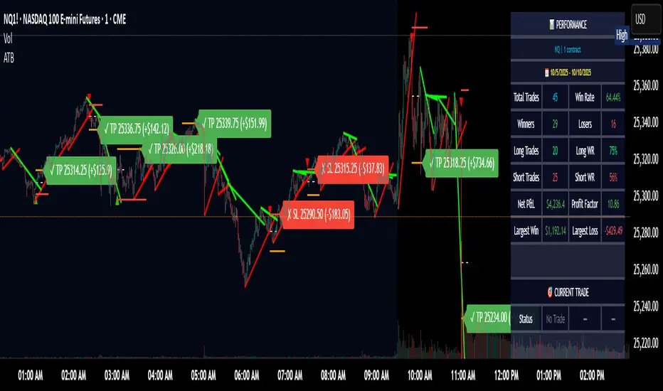
Adaptive Trend Breaks (ATB) is a trendline breakout system optimized for scalping liquid futures contracts. The indicator automatically draws dynamic support and resistance trendlines based on pivot points, then generates trade signals when price breaks through these levels with confirmation filters. It includes automated target and stop-loss placement with real-time P&L tracking in dollars.
## HOW IT WORKS
**Trendline Detection Method:**
The indicator uses pivot high/low detection to identify significant price turning points. When a new pivot forms, it calculates the slope between consecutive pivots to draw dynamic trendlines. These lines extend forward based on the established trend angle, creating actionable support and resistance zones.
**Band System:**
Around each trendline, the script creates a "band" using a volatility-adjusted calculation: `ATR(14) * 0.2 * bandwidth multiplier / 2`. This adaptive band accounts for current market conditions - wider during volatile periods, tighter during quiet markets.
**Breakout Logic:**
A breakout signal triggers when:
1. Price closes beyond the trendline + band zone
2. Volume exceeds the 20-period moving average by your set multiplier (default 1.2x)
3. Price is within Regular Trading Hours (9:30-16:00 EST) if session filter enabled
4. Current ATR meets minimum volatility threshold (prevents trading dead markets)
**Target & Stop Calculation:**
Upon breakout confirmation:
- **Entry**: Trendline breach point
- **Target**: Entry ± (bandwidth × target multiplier) - default 8x for quick scalps
- **Stop**: Entry ± (bandwidth × stop multiplier) - default 8x for 1:1 risk/reward
- Multipliers adjust automatically to market volatility through the ATR-based band
**P&L Conversion:**
The script converts point movements to dollars using:
```
Dollar P&L = (Price Points × Contract Point Value × Quantity)
```
For example, a 10-point NQ move with 2 contracts = 10 × $20 × 2 = $400
## HOW TO USE IT
**Setup:**
1. Select your instrument (NQ/ES/YM/RTY) - point values auto-configure
2. Set contract quantity for accurate dollar P&L
3. Choose pivot period (lower = more signals but more noise, default 5 for scalping)
4. Adjust bandwidth multiplier if trendlines are too tight/loose (1-5 range)
**Filters Configuration:**
- **Volume Filter**: Requires breakout volume > moving average × multiplier. Increase multiplier (1.5-2.0) for higher conviction trades
- **Session Filter**: Enable to trade only RTH. Disable for 24-hour trading
- **ATR Filter**: Prevents signals during low volatility. Increase minimum % for more active markets only
**Risk Management:**
- Set target/stop multipliers based on your risk tolerance
- 8x bandwidth = approximately 1:1 risk/reward for most liquid futures
- Enable trailing stops for trend-following approach (moves stop to protect profits)
- Adjust line length to see targets further into the future
**Statistics Table:**
- Choose timeframe to analyze: all-time, today, this week, custom days
- Monitor win rate, profit factor, and net P&L in dollars
- Track long vs short performance separately
- See real-time unrealized P&L on active trades
**Reading Signals:**
- **Green triangle below bar** = Long breakout (resistance broken)
- **Red triangle above bar** = Short breakout (support broken)
- **White dashed line** = Entry price
- **Orange line** = Take profit target with dollar value
- **Red line** = Stop loss with dollar value
- **Green checkmark (✓)** = Target hit, winning trade
- **Red X (✗)** = Stop hit, losing trade
## WHAT IT DOES NOT DO
**Limitations to Understand:**
- Does not predict future trendline formations - it reacts to breakouts after they occur
- Historical trendlines disappear after breakout (not kept on chart for clarity)
- Requires sufficient volatility - may not signal in extremely quiet markets
- Volume filter requires exchange volume data (not available on all symbols)
- Statistics are indicator-based simulations, not actual trading results
- Does not account for slippage, commissions, or order fills
## BEST PRACTICES
**Recommended Settings by Market:**
- **NQ (Nasdaq)**: Default settings work well, consider volume multiplier 1.3-1.5
- **ES (S&P 500)**: Slightly slower, try period 7-8, volume 1.2
- **YM (Dow)**: Lower volatility, reduce bandwidth to 1.5-2
- **RTY (Russell)**: Higher volatility, increase bandwidth to 3-4
**Risk Management:**
- Never risk more than 2-3% of account per trade
- Use contract quantity calculator: Max Risk $ ÷ (Stop Distance × Point Value)
- Start with 1 contract while learning the system
- Backtest your specific timeframe and instrument before live trading
**Optimization Tips:**
- Increase pivot period (7-10) for fewer but higher-quality signals
- Raise volume multiplier (1.5-2.0) in choppy markets
- Lower target/stop multipliers (5-6x) for tighter profit taking
- Use trailing stops in strong trending conditions
- Disable session filter for overnight gaps and Asia session moves
## TECHNICAL DETAILS
**Key Calculations:**
- Pivot Detection: `ta.pivothigh(high, period, period/2)` and `ta.pivotlow(low, period, period/2)`
- Slope Calculation: `(newPivot - oldPivot) / (newTime - oldTime)`
- Adaptive Band: `min(ATR(14) * 0.2, close * 0.002) * multiplier / 2`
- Breakout Confirmation: Price crosses trendline + 10% of band threshold
**Data Requirements:**
- Minimum bars in view: 500 for proper pivot calculation
- Volume data required for volume filter accuracy
- Intraday timeframes recommended (1min - 15min) for scalping
- Works on any timeframe but optimized for fast execution
**Performance Metrics:**
All statistics calculate based on indicator signals:
- Tracks every signal as a trade from entry to TP/SL
- P&L in actual contract dollar values
- Win rate = (Winning trades / Total trades) × 100
- Profit factor = Gross profit / Gross loss
- Separates long/short performance for bias analysis
## IDEAL FOR
- Futures scalpers and day traders
- Traders who prefer visual trendline breakouts
- Those wanting automated TP/SL placement
- Traders tracking performance in dollar terms
- Multiple timeframe analysis (compare 1min vs 5min signals)
## NOT SUITABLE FOR
- Swing trading (targets too close)
- Stocks/forex without modifying point values
- Extremely low timeframes (<30 seconds) - too much noise
- Markets without volume data if using volume filter
- Illiquid contracts (signals may not execute at shown prices)
---
**Settings Summary:**
- Core: Period, bandwidth, extension, trendline style
- Filters: Volume, RTH session, ATR volatility
- Risk: R:R ratio, target/stop multipliers, trailing stop
- Display: Stats table position, size, colors
- Stats: Timeframe selection (all-time to custom days)
**License:** This indicator is published open-source under Mozilla Public License 2.0. You may use and modify the code with proper attribution.
**Disclaimer:** This indicator is for educational purposes. Past performance does not guarantee future results. Always practice proper risk management and test thoroughly before live trading.
---
## CREDITS & ATTRIBUTION
This script builds upon the "Trendline Breakouts With Targets" concept by ChartPrime with significant enhancements:
**Major Improvements Added:**
- **Futures-Specific Calculations**: Automated dollar P&L conversion using actual contract point values (NQ=$20, ES=$50, YM=$5, RTY=$50)
- **Advanced Statistics Engine**: Comprehensive performance tracking with customizable timeframe analysis (today, week, month, custom ranges)
- **Multi-Layer Filtering System**: Volume confirmation, RTH session filter, and ATR volatility filter to reduce false signals
- **Professional Trade Management**: Enhanced visual trade tracking with separate TP/SL lines, dollar value labels, and optional trailing stops
- **Optimized for Scalping**: Faster pivot periods (5 vs 10), tighter bands, and reduced extension bars for quick entries
Original trendline detection methodology by ChartPrime - used with modification under Mozilla Public License 2.0.
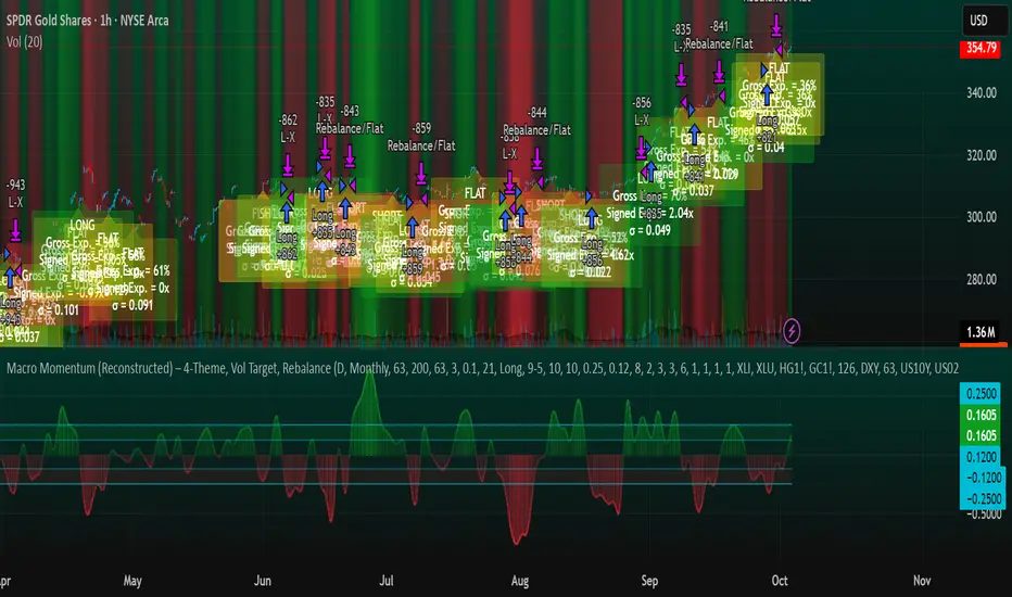
Macro Momentum – 4-Theme, Vol Target, RebalanceMacro Momentum — 4-Theme, Vol Target, Rebalance
Purpose. A macro-aware strategy that blends four economic “themes”—Business Cycle, Trade/USD, Monetary Policy, and Risk Sentiment—into a single, smoothed Composite signal. It then:
gates entries/exits with hysteresis bands,
enforces optional regime filters (200-day bias), and
sizes the position via volatility targeting with caps for long/short exposure.
It’s designed to run on any chart (index, ETF, futures, single stocks) while reading external macro proxies on a chosen Signal Timeframe.
How it works (high level)
Build four theme signals from robust macro proxies:
Business Cycle: XLI/XLU and Copper/Gold momentum, confirmed by the chart’s price vs a long SMA (default 200D).
Trade / USD: DXY momentum (sign-flipped so a rising USD is bearish for risk assets).
Monetary Policy: 10Y–2Y curve slope momentum and 10Y yield trend (steepening & falling 10Y = risk-on; rising 10Y = risk-off).
Risk Sentiment: VIX momentum (bearish if higher) and HYG/IEF momentum (bullish if credit outperforms duration).
Normalize & de-noise.
Optional Winsorization (MAD or stdev) clamps outliers over a lookback window.
Optional Z-score → tanh mapping compresses to ~ for stable weighting.
Theme lines are SMA-smoothed; the final Composite is LSMA-smoothed (linreg).
Decide direction with hysteresis.
Enter/hold long when Composite ≥ Entry Band; enter/hold short when Composite ≤ −Entry Band.
Exit bands are tighter than entry bands to avoid whipsaws.
Apply regime & direction constraints.
Optional Long-only above 200MA (chart symbol) and/or Short-only below 200MA.
Global Direction control (Long / Short / Both) and Invert switch.
Size via volatility targeting.
Realized close-to-close vol is annualized (choose 9-5 or 24/7 market profile).
Target exposure = TargetVol / RealizedVol, capped by Max Long/Max Short multipliers.
Quantity is computed from equity; futures are rounded to whole contracts.
Rebalance cadence & execution.
Trades are placed on Weekly / Monthly / Quarterly rebalance bars or when the sign of exposure flips.
Optional ATR stop/TP for single-stock style risk management.
Inputs you’ll actually tweak
General
Signal Timeframe: Where macro is sampled (e.g., D/W).
Rebalance Frequency: Weekly / Monthly / Quarterly.
ROC & SMA lengths: Defaults for theme momentum and the 200D regime filter.
Normalization: Z-score (tanh) on/off.
Winsorization
Toggle, lookback, multiplier, MAD vs Stdev.
Risk / Sizing
Target Annualized Vol & Realized Vol Lookback.
Direction (Long/Short/Both) and Invert.
Max long/short exposure caps.
Advanced Thresholds
Theme/Composite smoothing lengths.
Entry/Exit bands (hysteresis).
Regime / Execution
Long-only above 200MA, Short-only below 200MA.
Stops/TP (optional)
ATR length and SL/TP multiples.
Theme Weights
Per-theme scalars so you can push/pull emphasis (e.g., overweight Policy during rate cycles).
Macro Proxies
Symbols for each theme (XLI, XLU, HG1!, GC1!, DXY, US10Y, US02Y, VIX, HYG, IEF). Swap to alternatives as needed (e.g., UUP for DXY).
Signals & logic (under the hood)
Business Cycle = ½ ROC(XLI/XLU) + ½ ROC(Copper/Gold), then confirmed by (price > 200SMA ? +1 : −1).
Trade / USD = −ROC(DXY).
Monetary Policy = 0.6·ROC(10Y–2Y) − 0.4·ROC(10Y).
Risk Sentiment = −0.6·ROC(VIX) + 0.4·ROC(HYG/IEF).
Each theme → (optional Winsor) → (robust z or scaled ROC) → tanh → SMA smoothing.
Composite = weighted average → LSMA smoothing → compare to bands → dir ∈ {−1,0,+1}.
Rebalance & flips. Orders fire on your chosen cadence or when the sign of exposure changes.
Position size. exposure = clamp(TargetVol / realizedVol, maxLong/Short) × dir.
Note: The script also exposes Gross Exposure (% equity) and Signed Exposure (× equity) as diagnostics. These can help you audit how vol-targeting and caps translate into sizing over time.
Visuals & alerts
Composite line + columns (color/intensity reflect direction & strength).
Entry/Exit bands with green/red fills for quick polarity reads.
Hidden plots for each Theme if you want to show them.
Optional rebalance labels (direction, gross & signed exposure, σ).
Background heatmap keyed to Composite.
Alerts
Enter/Inc LONG when Composite crosses up (and on rebalance bars).
Enter/Inc SHORT when Composite crosses down (and on rebalance bars).
Exit to FLAT when Composite returns toward neutral (and on rebalance bars).
Practical tips
Start higher timeframes. Daily signals with Monthly rebalance are a good baseline; weekly signals with quarterly rebalances are even cleaner.
Tune Entry/Exit bands before anything else. Wider bands = fewer trades and less noise.
Weights reflect regime. If policy dominates markets, raise Monetary Policy weight; if credit stress drives moves, raise Risk Sentiment.
Proxies are swappable. Use UUP for USD, or futures-continuous symbols that match your data plan.
Futures vs ETFs. Quantity auto-rounds for futures; ETFs accept fractional shares. Check contract multipliers when interpreting exposure.
Caveats
Macro proxies can repaint at the selected signal timeframe as higher-TF bars form; that’s intentional for macro sampling, but test live.
Vol targeting assumes reasonably stationary realized vol over the lookback; if markets regime-shift, revisit volLook and targetVol.
If you disable normalization/winsorization, themes can become spikier; expect more hysteresis band crossings.
What to change first (quick start)
Set Signal Timeframe = D, Rebalance = Monthly, Z-score on, Winsor on (MAD).
Entry/Exit bands: 0.25 / 0.12 (defaults), then nudge until trade count and turnover feel right.
TargetVol: try 10% for diversified indices; lower for single stocks, higher for vol-sell strategies.
Leave weights = 1.0 until you’ve inspected the four theme lines; then tilt deliberately.
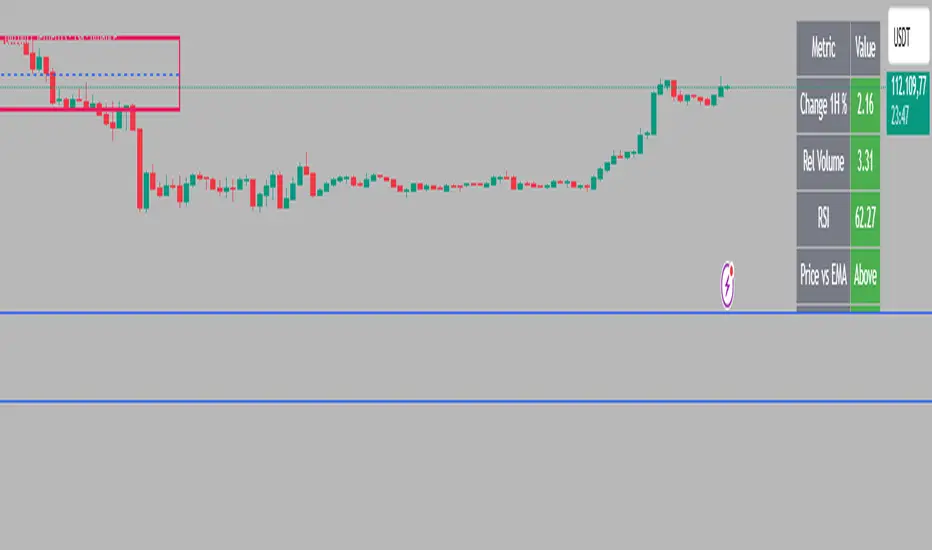
Intraday Rising & Reversal ScannerPine Script Description: Intraday Rising & Reversal ScannerThis Pine Script is a TradingView indicator designed to identify stocks with intraday (1-hour timeframe) potential for bullish (rising) or bearish (reversal) movements. It scans for stocks based on user-defined technical criteria, including price change, relative volume, RSI, EMA, ATR, and VWAP. The script plots signals on the chart, displays a summary table, and triggers alerts when conditions are met.FeaturesBullish Signal (Rising Stocks):1H Price Change: > 1% (configurable, e.g., >2% for volatile markets).
Relative Volume: > 2.0 (volume is at least twice the 20-period average).
RSI (14): Between 50 and 70 (strong but not overbought momentum).
Price vs EMA 13: Price above the 13-period EMA (confirms short-term uptrend).
ATR (14): Current ATR above its 20-period average (indicates volatility).
VWAP: Price above VWAP (optional, shown on chart for manual confirmation).
Bearish Signal (Reversal Stocks):1H Price Change: < -1% (configurable, e.g., <-2% for stronger reversals).
Relative Volume: > 2.0 (high volume confirms selling pressure).
RSI (14): > 70 (overbought, increasing reversal likelihood).
Price vs EMA 13: Price below the 13-period EMA (confirms short-term downtrend).
ATR (14): Current ATR above its 20-period average (indicates volatility).
VWAP: Price below VWAP (optional, shown on chart for manual confirmation).
Visualization:Bullish Signal: Green triangle below the bar.
Bearish Signal: Red triangle above the bar.
VWAP: Plotted as a blue line for manual verification.
Table: Displays real-time metrics (Change %, Relative Volume, RSI, Price vs EMA, ATR, VWAP) in the top-right corner, color-coded (green for bullish, red for bearish).
Alerts:Separate alerts for bullish ("Intraday Bullish Signal") and bearish ("Intraday Bearish Signal") conditions.
Customizable alert messages include parameter values for easy tracking.
How It WorksThe script runs on the 1-hour (1H) timeframe, ensuring all calculations are based on hourly data.
Indicators are computed:Change %: Percentage price change over the last hour.
Relative Volume: Current volume divided by the 20-period SMA of volume.
RSI: 14-period Relative Strength Index.
EMA 13: 13-period Exponential Moving Average.
ATR: 14-period Average True Range, compared to its 20-period SMA.
VWAP: Volume Weighted Average Price, plotted for visual confirmation.
Signals are generated when all conditions for either bullish or bearish criteria are met.
A table summarizes key metrics, and alerts can be set up for real-time notifications.
Usage InstructionsApply the Script:Open TradingView’s Pine Editor.
Copy and paste the script.
Click "Add to Chart" and set the chart to the 1-hour (1H) timeframe.
Set Up Alerts:Right-click on the chart > "Add Alert".
Select "Intraday Bullish Signal" or "Intraday Bearish Signal" as the condition.
Configure notifications (e.g., SMS, email, or TradingView alerts).
Manual VWAP Check:VWAP is plotted as a blue line. Verify that the price is above VWAP for bullish signals or below for bearish signals using the table or chart.
To make VWAP a mandatory filter, uncomment the VWAP conditions in the bull_signal and bear_signal definitions.
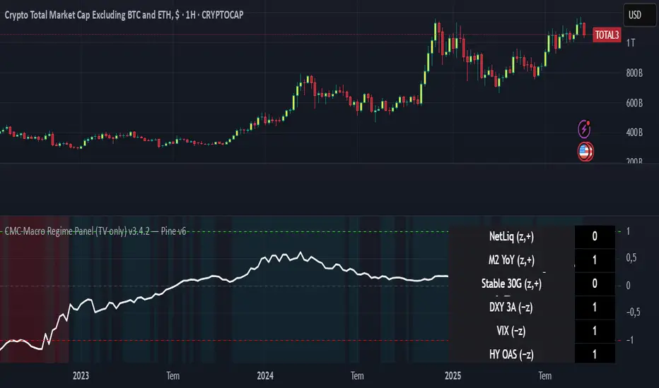
CMC Macro Regime PanelOverview (what it is):
A macro‑regime gate built entirely from TradingView-native symbols (CRYPTOCAP, FRED, DXY/VIX, HYG/LQD). It aggregates central‑bank liquidity (Fed balance sheet − RRP − Treasury General Account), USD strength, credit conditions, stablecoin flows/dominance, tech beta and BTC–NDX co‑move into one normalized score (CLRC). The panel outputs Risk‑ON/OFF regimes, an Early 3/5 pre‑signal, and an automatic BTC vs ETH vs ALTs preference. It is intentionally scoped to Daily & Weekly reads (no intraday timing). Publish with a clean chart and a clear description as per TradingView rules.
TradingView
Why we also use other TradingView screens (and why that is compliant)
This script pulls data via request.security() from official TV symbols only; users often want to open the raw series on separate charts to sanity‑check:
CRYPTOCAP indices: TOTAL, TOTAL2, TOTAL3 (market cap aggregates) and dominance tickers like BTC.D, USDT.D. Helpful for regime & rotation (ALTs vs BTC). TradingView provides definitions for crypto market cap and dominance symbols.
TradingView
+3
TradingView
+3
TradingView
+3
FRED releases: WALCL (Fed assets, weekly), RRPONTSYD (ON RRP, daily), WTREGEN (TGA, weekly), M2SL (M2, monthly). These are the official macro sources exposed on TV.
FRED
+3
FRED
+3
FRED
+3
Risk proxies: TVC:DXY (USD index), TVC:VIX (implied vol), AMEX:HYG/AMEX:LQD (credit), NASDAQ:NDX (tech beta), BINANCE:ETHBTC. VIX/NDX relationship is well-documented; VIX measures 30‑day expected S&P500 vol.
TradingView
+2
TradingView
+2
Compliance note: Using multiple screens is optional for users, but it explains/justifies how components work together (a requirement for public scripts). Keep publication chart clean; use extra screens only to illustrate in the description.
TradingView
How it works (high level)
Liquidity block (Weekly/Monthly)
Net Liquidity = WALCL − RRPONTSYD − WTREGEN (YoY z‑score). WALCL is weekly (as of Wednesday) via H.4.1; RRP is daily; TGA is a Fed liability series. M2 YoY is monthly.
FRED
+3
FRED
+3
FRED
+3
Risk conditions (Daily)
DXY 3‑month momentum (inverted), VIX level (inverted), Credit (HYG/LQD ratio or HY OAS). VIX is a 30‑day constant‑maturity implied vol index per Cboe methodology.
Cboe
+1
Crypto‑internal (Daily)
Stablecoins (USDT+USDC+DAI 30‑day log change), USDT dominance (20‑day, inverted), TOTAL3 (63‑day momentum). Dominance symbols on TV follow a documented formula.
TradingView
Beta & co‑move (Daily)
NDX 63‑day momentum, BTC↔NDX 90‑day correlation.
All components become z‑scores (optionally clipped), weighted, missing inputs drop and weights renormalize. We never use lookahead; we confirm on bar close to avoid repainting per Pine docs (barstate.isconfirmed, multi‑TF).
TradingView
+2
TradingView
+2
What you see on the chart
White line (CLRC) = macro regime score.
Background: Green = Risk‑ON, Red = Risk‑OFF, Teal = Early 3/5 (pre‑signal).
Table: shows each component’s z‑score and the Preference: BTC / ETH / ALTs / Mixed.
Signals & interpretation
Designed for Daily (1D) and Weekly (1W) only.
Regime gates (default Fast preset):
Enter ON: CLRC ≥ +0.8; Hold ON while ≥ +0.5.
Enter OFF: CLRC ≤ −1.0; Hold OFF while ≤ −0.5.
0 / ±1 reading: CLRC is a standardized composite.
~0 = neutral baseline (no macro edge).
≥ +1 = strong macro tailwind (≈ +1σ).
≤ −1 = strong headwind (≈ −1σ).
Early 3/5 (teal): a fast pre‑signal when at least 3 of 5 daily checks align: USDT.D↓, DXY↓, VIX↓, HYG/LQD↑, ETHBTC↑ or TOTAL3↑. It often precedes a full ON flip—use for pre‑positioning rather than full sizing.
BTC/ETH/ALTs selector (only when ON):
ALTs when BTC.D↓ and (ETHBTC↑ or TOTAL3↑) ⇒ rotate down the risk curve.
BTC when BTC.D↑ and ETHBTC↓ ⇒ keep it concentrated.
ETH when ETHBTC↑ while BTC.D flat/up ⇒ add ETH beta.
(Dominance mechanics are documented by TV.)
TradingView
Dissonance (incompatibility) rules — when to stand down
Use these overrides to avoid false comfort:
CLRC > +1 but USDT.D↑ and/or VIX spikes day‑over‑day → downgrade to Neutral; wait for USDT.D to stabilize and VIX to cool (VIX is a fear gauge of 30‑day expectation).
Cboe Global Markets
CLRC > +1 but DXY↑ sharply (USD squeeze) → size below normal; require DXY momentum to roll over.
CLRC < −1 but Early 3/5 = true two days in a row → start reducing underweights; look for ON flip within a few bars.
NetLiq improving (W) but credit (HYG/LQD) deteriorating (D) → treat as mixed regime; prefer BTC over ALTs.
How to use (step‑by‑step)
A. Read on Daily (1D) — main regime
Open CRYPTOCAP:TOTAL3, 1D (panel applied).
Wait for bar close (use alerts on confirmed bar). Pine docs recommend barstate.isconfirmed to avoid repainting on realtime bars.
TradingView
If ON, check Preference (BTC / ETH / ALTs).
Then drop to 4H on your trading pair for micro entries (this indicator itself is not for intraday timing).
B. Confirm weekly macro (1W) — once per week)
Review WALCL/RRP/TGA after the H.4.1 release on Thursdays ~4:30 pm ET. WALCL is “Weekly, as of Wednesday”; M2 is Monthly—so do not expect daily responsiveness from these.
Federal Reserve
+2
FRED
+2
Recommended check times (practical schedule)
Daily regime read: right after your chart’s daily close (confirmed bar). For consistent timing across crypto, many users set chart timezone to UTC and read ~00:05 UTC; you can change chart timezone in TV’s settings.
TradingView
In‑day monitoring: optional spot checks 16:00 & 20:00 UTC (DXY/VIX move during US hours), but act only after the daily bar confirms.
Weekly macro pass: Thu 21:30–22:30 UTC (after H.4.1 4:30 pm ET) or Fri after daily close, to let weekly FRED series propagate.
Federal Reserve
Limitations & data latency (be explicit)
Higher‑TF data & confirmation: FRED weekly/monthly series will not reflect intraday risk in crypto; we aggregate them for regime, not for entry timing.
Repainting 101: Realtime bars move until close. This script does not use lookahead and follows Pine guidance on multi‑TF series; still, always act on confirmed bars.
TradingView
+1
Public‑library compliance: Title EN‑only; description starts in EN; clean chart; justify component mash‑up; no lookahead; no unrealistic claims.
TradingView
Alerts you can use
“Macro Risk‑ON (entry)” — fires on ON flip (confirmed bar).
“Macro Risk‑OFF (entry)” — fires on OFF flip.
“Early 3/5” — fires when the teal pre‑signal appears (not a regime flip).
“Preference change” — BTC/ETH/ALTs toggles while ON.
Publish note: Alerts are fine; just avoid implying guaranteed accuracy/performance.
TradingView
Background research (why these inputs matter)
Liquidity → Crypto: Fed H.4.1 timing and series definitions (WALCL, RRP, TGA) formalize the “net liquidity” concept used here.
FRED
+3
Federal Reserve
+3
FRED
+3
Stablecoins ↔ Non‑stable crypto: empirical work shows bi‑directional causality between stablecoin market cap and non‑stable crypto cap; stablecoin growth co‑moves with broader crypto activity.
Global liquidity link: world liquidity positively relates to total crypto market cap; lagged effects are observed at monthly horizons.
VIX/Uncertainty effect: fear shocks impair BTC’s “safe haven” behavior; VIX is a meaningful risk‑off read.
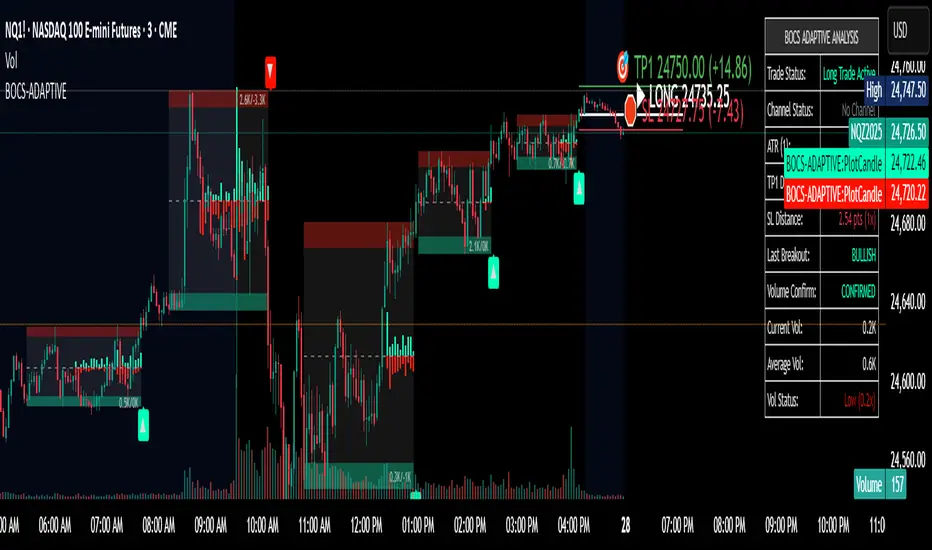
BOCS AdaptiveBOCS Adaptive Strategy - Automated Volatility Breakout System
WHAT THIS STRATEGY DOES:
This is an automated trading strategy that detects consolidation patterns through volatility analysis and executes trades when price breaks out of these channels. Take-profit and stop-loss levels are calculated dynamically using Average True Range (ATR) to adapt to current market volatility. The strategy closes positions partially at the first profit target and exits the remainder at the second target or stop loss.
TECHNICAL METHODOLOGY:
Price Normalization Process:
The strategy begins by normalizing price to create a consistent measurement scale. It calculates the highest high and lowest low over a user-defined lookback period (default 100 bars). The current close price is then normalized using the formula: (close - lowest_low) / (highest_high - lowest_low). This produces values between 0 and 1, allowing volatility analysis to work consistently across different instruments and price levels.
Volatility Detection:
A 14-period standard deviation is applied to the normalized price series. Standard deviation measures how much prices deviate from their average - higher values indicate volatility expansion, lower values indicate consolidation. The strategy uses ta.highestbars() and ta.lowestbars() functions to track when volatility reaches peaks and troughs over the detection length period (default 14 bars).
Channel Formation Logic:
When volatility crosses from a high level to a low level, this signals the beginning of a consolidation phase. The strategy records this moment using ta.crossover(upper, lower) and begins tracking the highest and lowest prices during the consolidation. These become the channel boundaries. The duration between the crossover and current bar must exceed 10 bars minimum to avoid false channels from brief volatility spikes. Channels are drawn using box objects with the recorded high/low boundaries.
Breakout Signal Generation:
Two detection modes are available:
Strong Closes Mode (default): Breakout occurs when the candle body midpoint math.avg(close, open) exceeds the channel boundary. This filters out wick-only breaks.
Any Touch Mode: Breakout occurs when the close price exceeds the boundary.
When price closes above the upper channel boundary, a bullish breakout signal generates. When price closes below the lower boundary, a bearish breakout signal generates. The channel is then removed from the chart.
ATR-Based Risk Management:
The strategy uses request.security() to fetch ATR values from a specified timeframe, which can differ from the chart timeframe. For example, on a 5-minute chart, you can use 1-minute ATR for more responsive calculations. The ATR is calculated using ta.atr(length) with a user-defined period (default 14).
Exit levels are calculated at the moment of breakout:
Long Entry Price = Upper channel boundary
Long TP1 = Entry + (ATR × TP1 Multiplier)
Long TP2 = Entry + (ATR × TP2 Multiplier)
Long SL = Entry - (ATR × SL Multiplier)
For short trades, the calculation inverts:
Short Entry Price = Lower channel boundary
Short TP1 = Entry - (ATR × TP1 Multiplier)
Short TP2 = Entry - (ATR × TP2 Multiplier)
Short SL = Entry + (ATR × SL Multiplier)
Trade Execution Logic:
When a breakout occurs, the strategy checks if trading hours filter is satisfied (if enabled) and if position size equals zero (no existing position). If volume confirmation is enabled, it also verifies that current volume exceeds 1.2 times the 20-period simple moving average.
If all conditions are met:
strategy.entry() opens a position using the user-defined number of contracts
strategy.exit() immediately places a stop loss order
The code monitors price against TP1 and TP2 levels on each bar
When price reaches TP1, strategy.close() closes the specified number of contracts (e.g., if you enter with 3 contracts and set TP1 close to 1, it closes 1 contract). When price reaches TP2, it closes all remaining contracts. If stop loss is hit first, the entire position exits via the strategy.exit() order.
Volume Analysis System:
The strategy uses ta.requestUpAndDownVolume(timeframe) to fetch up volume, down volume, and volume delta from a specified timeframe. Three display modes are available:
Volume Mode: Shows total volume as bars scaled relative to the 20-period average
Comparison Mode: Shows up volume and down volume as separate bars above/below the channel midline
Delta Mode: Shows net volume delta (up volume - down volume) as bars, positive values above midline, negative below
The volume confirmation logic compares breakout bar volume to the 20-period SMA. If volume ÷ average > 1.2, the breakout is classified as "confirmed." When volume confirmation is enabled in settings, only confirmed breakouts generate trades.
INPUT PARAMETERS:
Strategy Settings:
Number of Contracts: Fixed quantity to trade per signal (1-1000)
Require Volume Confirmation: Toggle to only trade signals with volume >120% of average
TP1 Close Contracts: Exact number of contracts to close at first target (1-1000)
Use Trading Hours Filter: Toggle to restrict trading to specified session
Trading Hours: Session input in HHMM-HHMM format (e.g., "0930-1600")
Main Settings:
Normalization Length: Lookback bars for high/low calculation (1-500, default 100)
Box Detection Length: Period for volatility peak/trough detection (1-100, default 14)
Strong Closes Only: Toggle between body midpoint vs close price for breakout detection
Nested Channels: Allow multiple overlapping channels vs single channel at a time
ATR TP/SL Settings:
ATR Timeframe: Source timeframe for ATR calculation (1, 5, 15, 60, etc.)
ATR Length: Smoothing period for ATR (1-100, default 14)
Take Profit 1 Multiplier: Distance from entry as multiple of ATR (0.1-10.0, default 2.0)
Take Profit 2 Multiplier: Distance from entry as multiple of ATR (0.1-10.0, default 3.0)
Stop Loss Multiplier: Distance from entry as multiple of ATR (0.1-10.0, default 1.0)
Enable Take Profit 2: Toggle second profit target on/off
VISUAL INDICATORS:
Channel boxes with semi-transparent fill showing consolidation zones
Green/red colored zones at channel boundaries indicating breakout areas
Volume bars displayed within channels using selected mode
TP/SL lines with labels showing both price level and distance in points
Entry signals marked with up/down triangles at breakout price
Strategy status table showing position, contracts, P&L, ATR values, and volume confirmation status
HOW TO USE:
For 2-Minute Scalping:
Set ATR Timeframe to "1" (1-minute), ATR Length to 12, TP1 Multiplier to 2.0, TP2 Multiplier to 3.0, SL Multiplier to 1.5. Enable volume confirmation and strong closes only. Use trading hours filter to avoid low-volume periods.
For 5-15 Minute Day Trading:
Set ATR Timeframe to match chart or use 5-minute, ATR Length to 14, TP1 Multiplier to 2.0, TP2 Multiplier to 3.5, SL Multiplier to 1.2. Volume confirmation recommended but optional.
For Hourly+ Swing Trading:
Set ATR Timeframe to 15-30 minute, ATR Length to 14-21, TP1 Multiplier to 2.5, TP2 Multiplier to 4.0, SL Multiplier to 1.5. Volume confirmation optional, nested channels can be enabled for multiple setups.
BACKTEST CONSIDERATIONS:
Strategy performs best during trending or volatility expansion phases
Consolidation-heavy or choppy markets produce more false signals
Shorter timeframes require wider stop loss multipliers due to noise
Commission and slippage significantly impact performance on sub-5-minute charts
Volume confirmation generally improves win rate but reduces trade frequency
ATR multipliers should be optimized for specific instrument characteristics
COMPATIBLE MARKETS:
Works on any instrument with price and volume data including forex pairs, stock indices, individual stocks, cryptocurrency, commodities, and futures contracts. Requires TradingView data feed that includes volume for volume confirmation features to function.
KNOWN LIMITATIONS:
Stop losses execute via strategy.exit() and may not fill at exact levels during gaps or extreme volatility
request.security() on lower timeframes requires higher-tier TradingView subscription
False breakouts inherent to breakout strategies cannot be completely eliminated
Performance varies significantly based on market regime (trending vs ranging)
Partial closing logic requires sufficient position size relative to TP1 close contracts setting
RISK DISCLOSURE:
Trading involves substantial risk of loss. Past performance of this or any strategy does not guarantee future results. This strategy is provided for educational purposes and automated backtesting. Thoroughly test on historical data and paper trade before risking real capital. Market conditions change and strategies that worked historically may fail in the future. Use appropriate position sizing and never risk more than you can afford to lose. Consider consulting a licensed financial advisor before making trading decisions.
ACKNOWLEDGMENT & CREDITS:
This strategy is built upon the channel detection methodology created by AlgoAlpha in the "Smart Money Breakout Channels" indicator. Full credit and appreciation to AlgoAlpha for pioneering the normalized volatility approach to identifying consolidation patterns and sharing this innovative technique with the TradingView community. The enhancements added to the original concept include automated trade execution, multi-timeframe ATR-based risk management, partial position closing by contract count, volume confirmation filtering, and real-time position monitoring.
Opening Range IndicatorComplete Trading Guide: Opening Range Breakout Strategy
What Are Opening Ranges?
Opening ranges capture the high and low prices during the first few minutes of market open. These levels often act as key support and resistance throughout the trading day because:
Heavy volume occurs at market open as overnight orders execute
Institutional activity is concentrated during opening minutes
Price discovery happens as market participants react to overnight news
Psychological levels are established that traders watch all day
Understanding the Three Timeframes
OR5 (5-Minute Range: 9:30-9:35 AM)
Most sensitive - captures immediate market reaction
Quick signals but higher false breakout rate
Best for scalping and momentum trading
Use for early entry when conviction is high
OR15 (15-Minute Range: 9:30-9:45 AM)
Balanced approach - most popular among day traders
Moderate sensitivity with better reliability
Good for swing trades lasting several hours
Primary timeframe for most strategies
OR30 (30-Minute Range: 9:30-10:00 AM)
Most reliable but slower signals
Lower false breakout rate
Best for position trades and trend following
Use when looking for major moves
Core Trading Strategies
Strategy 1: Basic Breakout
Setup:
Wait for price to break above OR15 high or below OR15 low
Enter on the breakout candle close
Stop loss: Opposite side of the range
Target: 2-3x the range size
Example:
OR15 range: $100.00 - $102.00 (Range = $2.00)
Long entry: Break above $102.00
Stop loss: $99.50 (below OR15 low)
Target: $104.00+ (2x range size)
Strategy 2: Multiple Confirmation
Setup:
Wait for OR5 break first (early signal)
Confirm with OR15 break in same direction
Enter on OR15 confirmation
Stop: Below OR30 if available, or OR15 opposite level
Why it works:
Multiple timeframe confirmation reduces false signals and increases probability of sustained moves.
Strategy 3: Failed Breakout Reversal
Setup:
Price breaks OR15 level but fails to hold
Wait for re-entry into the range
Enter reversal trade toward opposite OR level
Stop: Recent breakout high/low
Target: Opposite side of range + extension
Key insight: Failed breakouts often lead to strong moves in the opposite direction.
Advanced Techniques
Range Quality Assessment
High-Quality Ranges (Trade these):
Range size: 0.5% - 2% of stock price
Clean boundaries (not choppy)
Volume spike during range formation
Clear rejection at range levels
Low-Quality Ranges (Avoid these):
Very narrow ranges (<0.3% of stock price)
Extremely wide ranges (>3% of stock price)
Choppy, overlapping candles
Low volume during formation
Volume Confirmation
For Breakouts:
Look for volume spike (2x+ average) on breakout
Declining volume often signals false breakout
Rising volume during range formation shows interest
Market Context Filters
Best Conditions:
Trending market days (SPY/QQQ with clear direction)
Earnings reactions or news-driven moves
High-volume stocks with good liquidity
Volatility above average (VIX considerations)
Avoid Trading When:
Extremely low volume days
Major economic announcements pending
Holidays or half-days
Choppy, sideways market conditions
Risk Management Rules
Position Sizing
Conservative: Risk 0.5% of account per trade
Moderate: Risk 1% of account per trade
Aggressive: Risk 2% maximum per trade
Stop Loss Placement
Inside the range: Quick exit but higher stop-out rate
Outside opposite level: More room but larger risk
ATR-based: 1.5-2x Average True Range below entry
Profit Taking
Target 1: 1x range size (take 50% off)
Target 2: 2x range size (take 25% off)
Runner: Trail remaining 25% with moving stops
Specific Entry Techniques
Breakout Entry Methods
Method 1: Immediate Entry
Enter as soon as price closes above/below range
Fastest entry but highest false signal rate
Best for strong momentum situations
Method 2: Pullback Entry
Wait for breakout, then pullback to range level
Enter when price bounces off former resistance/support
Better risk/reward but may miss some moves
Method 3: Volume Confirmation
Wait for breakout + volume spike
Enter after volume confirmation candle
Reduces false signals significantly
Multiple Timeframe Entries
Aggressive: OR5 break → immediate entry
Conservative: OR5 + OR15 + OR30 all align → enter
Balanced: OR15 break with OR30 support → enter
Common Mistakes to Avoid
1. Trading Poor-Quality Ranges
❌ Don't trade ranges that are too narrow or too wide
✅ Focus on clean, well-defined ranges with good volume
2. Ignoring Volume
❌ Don't chase breakouts without volume confirmation
✅ Always check for volume spike on breakouts
3. Over-Trading
❌ Don't force trades when ranges are unclear
✅ Wait for high-probability setups only
4. Poor Risk Management
❌ Don't risk more than planned or use tight stops in volatile conditions
✅ Stick to predetermined risk levels
5. Fighting the Trend
❌ Don't fade breakouts in strongly trending markets
✅ Align trades with overall market direction
Daily Trading Routine
Pre-Market (8:00-9:30 AM)
Check overnight news and earnings
Review major indices (SPY, QQQ, IWM)
Identify potential opening range candidates
Set alerts for range breakouts
Market Open (9:30-10:00 AM)
Watch opening range formation
Note volume and price action quality
Mark key levels on charts
Prepare for breakout signals
Trading Session (10:00 AM - 4:00 PM)
Execute breakout strategies
Manage existing positions
Trail stops as profits develop
Look for additional setups
Post-Market Review
Analyze winning and losing trades
Review range quality vs. outcomes
Identify improvement areas
Prepare for next session
Best Stocks/ETFs for Opening Range Trading
Large Cap Stocks (Best for beginners):
AAPL, MSFT, GOOGL, AMZN, TSLA
High liquidity, predictable behavior
Good range formation most days
ETFs (Consistent patterns):
SPY, QQQ, IWM, XLF, XLE
Excellent liquidity
Clear range boundaries
Mid-Cap Growth (Advanced traders):
Stocks with good volume (1M+ shares daily)
Recent news catalysts
Clean technical patterns
Performance Optimization
Track These Metrics:
Win rate by range type (OR5 vs OR15 vs OR30)
Average R/R (risk vs reward ratio)
Best performing market conditions
Time of day performance
Continuous Improvement:
Keep detailed trade journal
Review failed breakouts for patterns
Adjust position sizing based on win rate
Refine entry timing based on backtesting
Final Tips for Success
Start small - Paper trade or use tiny positions initially
Focus on quality - Better to miss trades than take bad ones
Stay disciplined - Stick to your rules even during losing streaks
Adapt to conditions - What works in trending markets may fail in choppy conditions
Keep learning - Markets evolve, so should your approach
The opening range strategy is powerful because it captures natural market behavior, but like all strategies, it requires practice, discipline, and proper risk management to be profitable long-term.

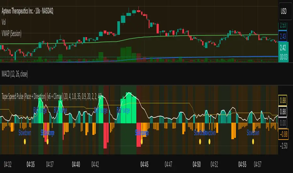
Tape Speed Pulse (Pace + Direction) [v6 + Climax]Tape Speed Pulse (Pace + Direction)
One-liner:
A lightweight “tape pulse” that turns intraday bursts of buying/selling into an easy-to-read histogram, with surge, slowdown, and climax (exhaustion) markers for fast decision-making. Use on sec and min charts.
What it measures
Pace (RVOL): current bar volume vs the recent average (smoothed).
Direction proxy: uptick/downtick by comparing close to close .
Pulse (histogram): direction × pace, so you see who’s pushing and how fast.
Colors
- Lime = Buy surge (pace ≥ threshold & upticking)
- Red = Sell surge (pace ≥ threshold & downticking)
- Teal = Buy pressure, sub-threshold
- Orange = Sell pressure, sub-threshold
- Faded/gray = Near-neutral pace (below the Neutral Band)
Lines (toggleable)
-White = Pace (RVOL)
- Yellow = Slowdown line = a drop of X% from the last 30-bar peak pace
Background tint mirrors the current state so you can glance risk: greenish for buy pressure, reddish for sell pressure.
Signals & alerts
- BUY surge – fires when pace crosses above the surge threshold with uptick direction (optional acceleration & uptick streak filters; cooldown prevents spam).
- SELL surge – mirror logic to downside.
- Slowdown – fires when pace crosses below the yellow slowdown line while direction ≤ 0 (early fade warning).
Climax (exhaustion)
- Buy Climax: previous bar was a buy surge with a large upper wick; current bar slows (below slowdown line) and direction ≤ 0.
- Sell Climax: mirror (large lower wick → slowdown → direction ≥ 0).
- Great for trimming/tight stops or fade setups at obvious spikes.
- Create alerts via Add alert → Condition: this indicator → choose the specific alert (BUY surge, SELL surge, Slowdown, Buy Climax, Sell Climax).
How to use it (playbook)
- Longs (e.g., VWAP reclaim / micro pullback)
- Only take entries when the pulse is teal→lime (buy pressure to buy surge).
- Into prior highs/VWAP bands, take partials on lime spikes.
- If you get a Slowdown dot and bars turn orange/red, tighten or exit.
Shorts (failed reclaim / lower-high)
- Look for teal→orange→red with rising pace at a level.
- Add confidence if a Buy Climax printed right before (exhaustion).
- Risk above the spike; don’t fight true ignitions out of bases.
Simple guardrails
- Avoid new longs when the histogram is orange/red; avoid new shorts when teal/lime.
- Use with VWAP + 9/20 EMA or your levels. The pulse is confirmation, not the whole thesis.
Inputs (what they do & when to tweak)
- Pace lookback (bars) – window for average volume. Lower = faster; higher = steadier.
Too jumpy? raise it. Missing quick bursts? lower it.
- Smoothing EMA (bars) – smooths pace. Higher = calmer.
Use 4–6 during the open; 3–4 midday.
- Surge threshold (× RVOL) – how fast counts as a surge.
Too many surges? raise it. Too late? lower it slightly.
- Slowdown drop from 30-bar max (%) – how far below the recent peak pace to call a slowdown.
Higher % = later slowdown; lower % = earlier warning.
- Neutral band (× RVOL) – paces below this fade to gray.
Raise to clean up noise; lower to see subtle pressure.
- Min seconds between signals – cooldown to prevent spam.
Increase in chop; reduce if you want more pings.
- BUY/SELL: min consecutive upticks/downticks – tiny streak filter.
Raise to avoid wiggles; lower for earlier signals.
Require pace accelerating into signal – ON = avoid stall breakouts; OFF = earlier pings.
Climax options: wick % threshold & “require slowdown cross”.
Raise wick% / require cross to be stricter; lower to catch more fades.
Quick presets
- Low-float runner, 5–10s chart
- Lookback 20, Smoothing 3–4, Surge 2.2–2.8, Slowdown 35–45, Neutral 1.0–1.2, Cooldown 15–25s, Streaks 2–3, Accel ON.
- Thick large-cap, 1-min
- Lookback 20–30, Smoothing 5–7, Surge 1.5–1.9, Slowdown 25–35, Neutral 0.8–1.0, Cooldown 30–60s, Streaks 2, Accel ON.
- Open vs Midday vs Power Hour
- Open: higher Surge, more Smoothing, longer Cooldown.
- Midday: lower Surge, less Smoothing to catch subtler pushes.
- Power hour: moderate Surge; keep Slowdown on for exits.
Reading common patterns
- Ignition (likely continuation): lime spike out of a base that holds above a level while pace stays above yellow.
- Exhaustion (likely fade): lime spike late in a run with upper wick → Slowdown → orange/red. The Buy Climax diamond is your tell.
Limits / notes
This is an OHLCV-based proxy (TradingView Pine can’t read raw tape/DOM). It won’t match Bookmap/Jigsaw tick-for-tick, but it’s fast and objective.
Use with levels and a risk plan. Past performance ≠ future results. Educational only.
MAxRSI Signals [KedArc Quant]Description:
MAxRSI Indicator Marks LONG/SHORT signals from a Moving Average crossover and (optionally) confirms them with RSI. Includes repaint-safe confirmation, optional higher-timeframe (HTF) smoothing, bar coloring, and alert conditions.
Why combine MA + RSI
* The MA crossover is the primary trend signal (fast trend vs slow trend).
* RSI is a gate, not a second, separate signal. A crossover only becomes a trade signal if momentum agrees (e.g., RSI ≥ level for LONG, ≤ level for SHORT). This reduces weak crosses in ranging markets.
* The parts are integrated in one rule: *Crossover AND RSI condition (if enabled)* → plot signal/alert. No duplicated outputs or unrelated indicators.
How it works (logic)
* MA types: SMA / EMA / WMA / HMA (HMA is built via WMA of `len/2` and `len`, then WMA with `sqrt(len)`).
* Signals:
* LONG when *Fast MA crosses above Slow MA* and (if enabled) *RSI ≥ Long Min*.
* SHORT when *Fast MA crosses below Slow MA* and (if enabled) *RSI ≤ Short Max*.
* Repaint-safe (optional): confirms crosses on closed bars to avoid intrabar repaint.
* HTF (optional): computes MA/RSI on a higher timeframe to smooth noise on lower charts.
* Alerts: crossover alerts + state-flip (bull↔bear) alerts.
How to use (step-by-step)
1. Add to chart. Set MA Type, Fast and Slow (keep Fast < Slow).
2. Turn Use RSI Filter ON for confirmation (default: RSI 14 with 50/50 levels).
3. (Optional) Turn Repaint-Safe ON for close-confirmed signals.
4. (Optional) Turn HTF ON (e.g., 60 = 1h) for smoother signals on low TFs.
5. Enable alerts: pick “MAxRSI Long/Short” or “Bullish/Bearish State”.
Timeframe guidance
* Intraday (1–15m): EMA 9–20 fast vs EMA 50 slow, RSI filter at 50/50.
* Swing (1h–D): EMA 20 fast vs EMA 200 slow, RSI 50/50 (55/45 for stricter).
What makes it original
* Repaint-safe cross confirmation (previous-bar check) for reliable signals/alerts.
* HTF gating (doesn’t compute both branches) for speed and clarity.
* Warning-free MA helper (precomputes SMA/EMA/WMA/HMA each bar), HMA built from built-ins only.
* State-flip alerts and optional RSI overlay on price pane.
Built-ins used
`ta.sma`, `ta.ema`, `ta.wma`, (HMA built from these), `ta.rsi`, `ta.crossover`, `ta.crossunder`, `request.security`, `plot`, `plotshape`, `barcolor`, `alertcondition`, `input.*`, `math.*`.
Note: Indicator only (no orders). Test settings per symbol. Not financial advice.
⚠️ Disclaimer
This script is provided for educational purposes only.
Past performance does not guarantee future results.
Trading involves risk, and users should exercise caution and use proper risk management when applying this strategy.

RSI ADX Bollinger Analysis High-level purpose and design philosophy
This indicator — RSI-ADX-Bollinger Analysis — is a compact, educational market-analysis toolkit that blends momentum (RSI), trend strength (ADX), volatility structure (Bollinger Bands) and simple volumetrics to provide traders a snapshot of market condition and trade idea quality. The design philosophy is explicit and layered: use each component to answer a different question about price action (momentum, conviction, volatility, participation), then combine answers to form a more robust, explainable signal. The mashup is intended for analysis and learning, not automatic execution: it surfaces the why behind signals so traders can test, learn and apply rules with risk management.
________________________________________
What each indicator contributes (component-by-component)
RSI (Relative Strength Index) — role and behavior: RSI measures short-term momentum by comparing recent gains to recent losses. A high RSI (near or above the overbought threshold) indicates strong recent buying pressure and potential exhaustion if price is extended. A low RSI (near or below the oversold threshold) indicates strong recent selling pressure and potential exhaustion or a value area for mean-reversion. In this dashboard RSI is used as the primary momentum trigger: it helps identify whether price is locally over-extended on the buy or sell side.
ADX (Average Directional Index) — role and behavior: ADX measures trend strength independently of direction. When ADX rises above a chosen threshold (e.g., 25), it signals that the market is trending with conviction; ADX below the threshold suggests range or weak trend. Because patterns and momentum signals perform differently in trending vs. ranging markets, ADX is used here as a filter: only when ADX indicates sufficient directional strength does the system treat RSI+BB breakouts as meaningful trade candidates.
Bollinger Bands — role and behavior: Bollinger Bands (20-period basis ± N standard deviations) show volatility envelope and relative price position vs. a volatility-adjusted mean. Price outside the upper band suggests pronounced extension relative to recent volatility; price outside the lower band suggests extended weakness. A band expansion (increasing width) signals volatility breakout potential; contraction signals range-bound conditions and potential squeeze. In this dashboard, Bollinger Bands provide the volatility/structural context: RSI extremes plus price beyond the band imply a stronger, volatility-backed move.
Volume split & basic MA trend — role and behavior: Buy-like and sell-like volume (simple heuristic using close>open or closeopen) or sell-like (close1.2 for validation and compare win rate and expectancy.
4. TF alignment: Accept signals only when higher timeframe (e.g., 4h) trend agrees — compare results.
5. Parameter sensitivity: Vary RSI threshold (70/30 vs 80/20), Bollinger stddev (2 vs 2.5), and ADX threshold (25 vs 30) and measure stability of results.
These exercises teach both statistical thinking and the specific failure modes of the mashup.
________________________________________
Limitations, failure modes and caveats (explicit & teachable)
• ADX and Bollinger measures lag during fast-moving news events — signals can be late or wrong during earnings, macro shocks, or illiquid sessions.
• Volume classification by open/close is a heuristic; it does not equal TAPEDATA, footprint or signed volume. Use it as supportive evidence, not definitive proof.
• RSI can remain overbought or oversold for extended stretches in persistent trends — relying solely on RSI extremes without ADX or BB context invites large drawdowns.
• Small-cap or low-liquidity instruments yield noisy band behavior and unreliable volume ratios.
Being explicit about these limitations is a strong point in a TradingView description — it demonstrates transparency and educational intent.
________________________________________
Originality & mashup justification (text you can paste)
This script intentionally combines classical momentum (RSI), volatility envelope (Bollinger Bands) and trend-strength (ADX) because each indicator answers a different and complementary question: RSI answers is price locally extreme?, Bollinger answers is price outside normal volatility?, and ADX answers is the market moving with conviction?. Volume participation then acts as a practical check for real market involvement. This combination is not a simple “indicator mashup”; it is a designed ensemble where each element reduces the others’ failure modes and together produce a teachable, testable signal framework. The script’s purpose is educational and analytical — to show traders how to interpret the interplay of momentum, volatility, and trend strength.
________________________________________
TradingView publication guidance & compliance checklist
To satisfy TradingView rules about mashups and descriptions, include the following items in your script description (without exposing source code):
1. Purpose statement: One or two lines describing the script’s objective (educational multi-indicator market overview and idea filter).
2. Component list: Name the major modules (RSI, Bollinger Bands, ADX, volume heuristic, SMA trend checks, signal tracking) and one-sentence reason for each.
3. How they interact: A succinct non-code explanation: “RSI finds momentum extremes; Bollinger confirms volatility expansion; ADX confirms trend strength; all three must align for a BUY/SELL.”
4. Inputs: List adjustable inputs (RSI length and thresholds, BB length & stddev, ADX threshold & smoothing, volume MA, table position/size).
5. Usage instructions: Short workflow (check TF alignment → confirm participation → define stop & R:R → backtest).
6. Limitations & assumptions: Explicitly state volume is approximated, ADX has lag, and avoid promising guaranteed profits.
7. Non-promotional language: No external contact info, ads, claims of exclusivity or guaranteed outcomes.
8. Trademark clause: If you used trademark symbols, remove or provide registration proof.
9. Risk disclaimer: Add the copy-ready disclaimer below.
This matches TradingView’s request for meaningful descriptions that explain originality and inter-component reasoning.
________________________________________
Copy-ready short publication description (paste into TradingView)
Advanced RSI-ADX-Bollinger Market Overview — educational multi-indicator dashboard. This script combines RSI (momentum extremes), Bollinger Bands (volatility envelope and band expansion), ADX (trend strength), simple SMA trend bias and a basic buy/sell volume heuristic to surface high-quality idea candidates. Signals require alignment of momentum, volatility expansion and rising ADX; volume participation is displayed to support signal confidence. Inputs are configurable (RSI length/levels, BB length/stddev, ADX length/threshold, volume MA, display options). This tool is intended for analysis and learning — not for automated execution. Users should back test and apply robust risk management. Limitations: volume classification here is a heuristic (close>open), ADX and BB measures lag in fast news events, and results vary by instrument liquidity.
________________________________________
Copy-ready risk & misuse disclaimer (paste into description or help file)
This script is provided for educational and analytical purposes only and does not constitute financial or investment advice. It does not guarantee profits. Indicators are heuristics and may give false or late signals; always back test and paper-trade before using real capital. The author is not responsible for trading losses resulting from the use or misuse of this indicator. Use proper position sizing and risk controls.
________________________________________
Risk Disclaimer: This tool is provided for education and analysis only. It is not financial advice and does not guarantee returns. Users assume all risk for trades made based on this script. Back test thoroughly and use proper risk management.
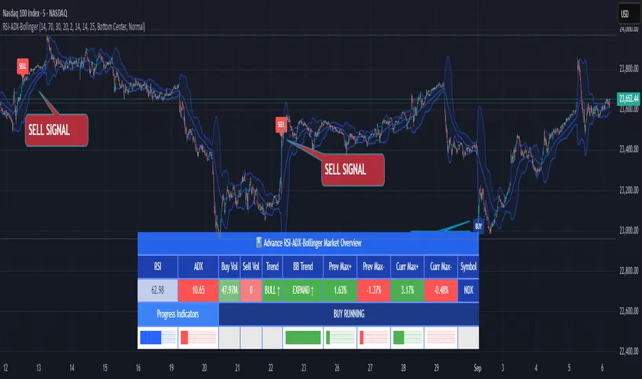
Savitzky-Golay Hampel Filter | AlphaNattSavitzky-Golay Hampel Filter | AlphaNatt
A revolutionary indicator combining NASA's satellite data processing algorithms with robust statistical outlier detection to create the most scientifically advanced trend filter available on TradingView.
"This is the same mathematics that processes signals from the Hubble Space Telescope and analyzes data from the Large Hadron Collider - now applied to financial markets."
━━━━━━━━━━━━━━━━━━━━━━━━━━━━━━━━━━━━━━━━
🚀 SCIENTIFIC PEDIGREE
Savitzky-Golay Filter Applications:
NASA: Satellite telemetry and space probe data processing
CERN: Particle physics data analysis at the LHC
Pharmaceutical: Chromatography and spectroscopy analysis
Astronomy: Processing signals from radio telescopes
Medical: ECG and EEG signal processing
Hampel Filter Usage:
Aerospace: Cleaning sensor data from aircraft and spacecraft
Manufacturing: Quality control in precision engineering
Seismology: Earthquake detection and analysis
Robotics: Sensor fusion and noise reduction
━━━━━━━━━━━━━━━━━━━━━━━━━━━━━━━━━━━━━━━━
🧬 THE MATHEMATICS
1. Savitzky-Golay Filter
The SG filter performs local polynomial regression on data points:
Fits a polynomial of degree n to a sliding window of data
Evaluates the polynomial at the center point
Preserves higher moments (peaks, valleys) unlike moving averages
Maintains derivative information for true momentum analysis
Originally published in Analytical Chemistry (1964)
Mathematical Properties:
Optimal smoothing in the least-squares sense
Preserves statistical moments up to polynomial order
Exact derivative calculation without additional lag
Superior frequency response vs traditional filters
2. Hampel Filter
A robust outlier detector based on Median Absolute Deviation (MAD):
Identifies outliers using robust statistics
Replaces spurious values with polynomial-fitted estimates
Resistant to up to 50% contaminated data
MAD is 1.4826 times more robust than standard deviation
Outlier Detection Formula:
|x - median| > k × 1.4826 × MAD
Where k is the threshold parameter (typically 3 for 99.7% confidence)
━━━━━━━━━━━━━━━━━━━━━━━━━━━━━━━━━━━━━━━━
💎 WHY THIS IS SUPERIOR
vs Moving Averages:
Preserves peaks and valleys (critical for catching tops/bottoms)
No lag penalty for smoothness
Maintains derivative information
Polynomial fitting > simple averaging
vs Other Filters:
Outlier immunity (Hampel component)
Scientifically optimal smoothing
Preserves higher-order features
Used in billion-dollar research projects
Unique Advantages:
Feature Preservation: Maintains market structure while smoothing
Spike Immunity: Ignores false breakouts and stop hunts
Derivative Accuracy: True momentum without additional indicators
Scientific Validation: 60+ years of academic research
━━━━━━━━━━━━━━━━━━━━━━━━━━━━━━━━━━━━━━━━
⚙️ PARAMETER OPTIMIZATION
1. Polynomial Order (2-5)
2 (Quadratic): Maximum smoothing, gentle curves
3 (Cubic): Balanced smoothing and responsiveness (recommended)
4-5 (Higher): More responsive, preserves more features
2. Window Size (7-51)
Must be odd number
Larger = smoother but more lag
Formula: 2×(desired smoothing period) + 1
Default 21 = analyzes 10 bars each side
3. Hampel Threshold (1.0-5.0)
1.0: Aggressive outlier removal (68% confidence)
2.0: Moderate outlier removal (95% confidence)
3.0: Conservative outlier removal (99.7% confidence) (default)
4.0+: Only extreme outliers removed
4. Final Smoothing (1-7)
Additional WMA smoothing after filtering
1 = No additional smoothing
3-5 = Recommended for most timeframes
7 = Ultra-smooth for position trading
━━━━━━━━━━━━━━━━━━━━━━━━━━━━━━━━━━━━━━━━
📊 TRADING STRATEGIES
Signal Recognition:
Cyan Line: Bullish trend with positive derivative
Pink Line: Bearish trend with negative derivative
Color Change: Trend reversal with polynomial confirmation
1. Trend Following Strategy
Enter when price crosses above cyan filter
Exit when filter turns pink
Use filter as dynamic stop loss
Best in trending markets
2. Mean Reversion Strategy
Enter long when price touches filter from below in uptrend
Enter short when price touches filter from above in downtrend
Exit at opposite band or filter color change
Excellent for range-bound markets
3. Derivative Strategy (Advanced)
The SG filter preserves derivative information
Acceleration = second derivative > 0
Enter on positive first derivative + positive acceleration
Exit on negative second derivative (momentum slowing)
━━━━━━━━━━━━━━━━━━━━━━━━━━━━━━━━━━━━━━━━
📈 PERFORMANCE CHARACTERISTICS
Strengths:
Outlier Immunity: Ignores stop hunts and flash crashes
Feature Preservation: Catches tops/bottoms better than MAs
Smooth Output: Reduces whipsaws significantly
Scientific Basis: Not curve-fitted or optimized to markets
Considerations:
Slight lag in extreme volatility (all filters have this)
Requires odd window sizes (mathematical requirement)
More complex than simple moving averages
Best with liquid instruments
━━━━━━━━━━━━━━━━━━━━━━━━━━━━━━━━━━━━━━━━
🔬 SCIENTIFIC BACKGROUND
Savitzky-Golay Publication:
"Smoothing and Differentiation of Data by Simplified Least Squares Procedures"
- Abraham Savitzky & Marcel Golay
- Analytical Chemistry, Vol. 36, No. 8, 1964
Hampel Filter Origin:
"Robust Statistics: The Approach Based on Influence Functions"
- Frank Hampel et al., 1986
- Princeton University Press
These techniques have been validated in thousands of scientific papers and are standard tools in:
NASA's Jet Propulsion Laboratory
European Space Agency
CERN (Large Hadron Collider)
MIT Lincoln Laboratory
Max Planck Institutes
━━━━━━━━━━━━━━━━━━━━━━━━━━━━━━━━━━━━━━━━
💡 ADVANCED TIPS
News Trading: Lower Hampel threshold before major events to catch spikes
Scalping: Use Order=2 for maximum smoothness, Window=11 for responsiveness
Position Trading: Increase Window to 31+ for long-term trends
Combine with Volume: Strong trends need volume confirmation
Multiple Timeframes: Use daily for trend, hourly for entry
Watch the Derivative: Filter color changes when first derivative changes sign
━━━━━━━━━━━━━━━━━━━━━━━━━━━━━━━━━━━━━━━━
⚠️ IMPORTANT NOTICES
Not financial advice - educational purposes only
Past performance does not guarantee future results
Always use proper risk management
Test settings on your specific instrument and timeframe
No indicator is perfect - part of complete trading system
━━━━━━━━━━━━━━━━━━━━━━━━━━━━━━━━━━━━━━━━
🏆 CONCLUSION
The Savitzky-Golay Hampel Filter represents the pinnacle of scientific signal processing applied to financial markets. By combining polynomial regression with robust outlier detection, traders gain access to the same mathematical tools that:
Guide spacecraft to other planets
Detect gravitational waves from black holes
Analyze particle collisions at near light-speed
Process signals from deep space
This isn't just another indicator - it's rocket science for trading .
"When NASA needs to separate signal from noise in billion-dollar missions, they use these exact algorithms. Now you can too."
━━━━━━━━━━━━━━━━━━━━━━━━━━━━━━━━━━━━━━━━
Developed by AlphaNatt
Version: 1.0
Release: 2025
Pine Script: v6
"Where Space Technology Meets Market Analysis"
Not financial advice. Always DYOR
Artharjan ADXArtharjan ADX (AADX) by Rrahul Desai @Artharjan
📌 Overview
The Artharjan ADX (AADX) is an advanced implementation of the Average Directional Index (ADX) with customizable moving averages, momentum thresholds, and visually intuitive grading of bullish and bearish strength.
Unlike the standard ADX indicator that only shows trend strength, AADX adds graded bullish/bearish conditions, alerts, smoothed DI signals, histogram visualizations, and background color fills to help traders quickly interpret market conditions.
It is designed for traders who want early detection of trend strength, clean visual cues, and automated alert triggers for both bullish and bearish momentum setups.
⚙️ Key Features
🔹 Customizable Calculations
DI Length (default 13) – controls sensitivity of directional indicators.
+/- DI Smoothing – smooths DI signals with user-selected MA.
Multiple Moving Average Types – SMA, EMA, WMA, RMA, VWMA, ALMA, Hull, SWMA, SMMA, TMA.
ADX Smoothing – define how smooth/fast the ADX reacts.
🔹 Flexible Display
Toggle between line plots or histogram view.
Adjustable plot thickness.
Option to plot averages of ADX, +DI, -DI for confirmation.
Configurable background fills:
ADX above/below momentum threshold.
ADX rising/falling color shading.
Trend-grade based color intensity.
🔹 Momentum & Thresholds
Momentum Level (default 25) → defines “strong trend” zone.
Crossover Threshold (default 15) → helps detect early DI crossovers.
Color-coded histogram bars for +DI vs -DI difference:
Above/below zero.
Rising/falling momentum.
🔹 Bullish & Bearish Grading System
The indicator assigns grades from 1 to 5 for both bullish and bearish setups, based on DI and ADX conditions:
Bullish Grades
Grade 1 → Very Weak Bullish
Grade 2 → Weak Bullish
Grade 3 → Moderate Bullish
Grade 4 → Strong Bullish
Grade 5 → Very Strong Bullish
Bearish Grades
Grade 1 → Very Weak Bearish
Grade 2 → Weak Bearish
Grade 3 → Moderate Bearish
Grade 4 → Strong Bearish
Grade 5 → Very Strong Bearish
Labels are automatically plotted above bars to indicate the active grade.
🔹 Alerts
Bullish Alert → when +DI crosses above its average below the threshold OR bullish conditions are met.
Bearish Alert → when -DI crosses above its average below the threshold OR bearish conditions are met.
These alerts make it possible to automate trading signals for scalping, intraday, and swing trading.
📊 Use Cases
Trend Strength Measurement
Spot when markets shift from range-bound to trending.
Confirm the reliability of breakouts with strong ADX readings.
Bullish vs Bearish Control
Compare +DI vs -DI strength to gauge trend direction.
Identify trend reversals early with DI slope changes.
Momentum Confirmation
Use ADX rising + DI grades to validate trade entries.
Filter false breakouts with weak ADX.
Trade Grading System
Enter aggressively on Grade 4–5 signals.
Stay cautious on Grade 1–2 signals.
Automated Alerts & Screening
Combine AADX alerts with strategy rules.
Build scanners to highlight strong ADX setups across multiple stocks.
🎯 Trader’s Advantage
More powerful than standard ADX → Adds slope, grading, alerts, and visualization.
Adaptable to any style → Works for intraday scalping, swing trading, and positional analysis.
Visual clarity → Color fills, histograms, and labels simplify decision-making.
Customizable smoothing → Adjusts to fast or slow markets.
✅ Closing Note
The Artharjan ADX (AADX) transforms the traditional ADX into a complete trend and momentum analyzer. It helps traders detect, confirm, and act on directional strength with clarity and confidence.
With Thanks,
Rrahul Desai
@Artharjan
RS Alpha by The Noiseless TraderRS Alpha by The Noiseless Trader plots a clean, benchmark‑relative strength line for any symbol and (optionally) a mean line to assess trend and momentum in relative performance. It’s designed for uncluttered, professional RS analysis and works across any timeframe.
Compare any symbol vs a benchmark (default: NSE:NIFTY).
Optional log‑normalized RS for return‑aware comparisons.
Optional RS Mean with trend coloring (rising/falling).
Optional RS Trend zero‑line coloring based on short‑range slope.
Lightweight alerts for rising/falling RS mean.
Tip: Use RS to identify leaders (RS > 0 with rising mean) and laggards (RS < 0 with falling mean), then align setups with your price action rules.
Reading the indicator
Leadership: RS > 0 and RS Mean rising → outperformance vs benchmark.
Weakness: RS < 0 and RS Mean falling → underperformance vs benchmark.
Inflections: Watch RS crossing above/below its Mean for early shifts.
Zero‑line context: With RS Trend on, the zero line subtly reflects short‑term slope (green for positive, maroon for negative).
Alerts
Rising Strength – RS Mean turning/remaining upward.
Declining Strength – RS Mean turning/remaining downward.
(Use these as context; execute entries on your price‑action rules.)
Best practices
Pair RS with your trend/structure rules (e.g., higher highs + RS leadership).
For sectors/baskets, keep the Comparative Symbol consistent to rank peers.
Log‑normalized RS helps when comparing assets with very different volatilities or large base effects.
Test multiple length and Mean settings; 60 is a balanced default for swing/positional work.
Credits
Original concept & code: © bharatTrader
Modifications & refinements: The Noiseless Trader
Elliott Wave Rule EngineWhat this tool does
The indicator scans price for two concurrent swing structures—a Small (shorter-degree) and a Large (higher-degree) set—then applies an Elliott/NeoWave rule engine to the most recent 5-swing motive (1-2-3-4-5) or 3-swing corrective (A-B-C). It produces:
Blue lines for Small swings and Orange lines for Large swings.
A rule dashboard (optional) showing PASS/FAIL/WARN for core rules & guidelines.
Buy/Sell labels when (a) a valid motive completes and (b) loop “consensus,” alignment, and scoring gates are satisfied.
Reading the chart
Small swings: thin blue segments, built from your Small settings.
Large swings: thicker orange segments, from your Large settings.
Background tint: faint green when a motive (impulse/diagonal) is valid right now on Small.
Labels (if enabled):
“1…5” or “A-B-C” markers on the latest detected structure.
Buy/Sell label at the last pivot when all gates pass; text may include a score %.
How it works
For both Small and Large degrees the script:
- Loops over all (left, right) combinations you specify (e.g., Small Left = 3..6, Right = 0..0) and calls ta.pivothigh/low.
- Aggregates the results:
- Keeps the most extreme pivot found in the loop (highest high or lowest low) that’s newer than the last accepted swing.
- Gates acceptance by minimum % change versus the last opposite swing (inside the loop) and a post-aggregation filter (Small Minimum swing %, Large Minimum swing %).
- Merges back-to-back same-type swings (HH or LL) by keeping only the more extreme one.
- Keeps only the last N=lookbackWaves swings (default 100).
- Consensus (used for signals) comes from the loop counts:
- sBuyConsensus = small L-count / total-combos (bullish bias)
- sSellConsensus = small H-count / total-combos (bearish bias)
(and the same for Large). This is a data-driven “how many combos agreed” measure.
2) Rule engine (Impulse/Diagonal vs. Corrective)
When there are at least 6 Small swings, the engine tests 1-2-3-4-5:
Hard rules (must pass for an Impulse):
- Wave-2 not > 100% of Wave-1 (no retrace beyond start of W1).
- Wave-3 not the shortest among 1,3,5.
- Wave-4 doesn’t overlap Wave-1 (if it does, structure may be a Diagonal).
- Diagonal eligibility: Rules 1 & 2 pass but Rule 3 fails ⇒ eligible as a Diagonal (
Guidelines (7 checks, count toward a threshold you set):
- W2 retraces a Fib level (within ±fibTol).
- W4 retraces a Fib level (within ±fibTol).
- W3 strongest momentum (speed = |Δprice| / bars).
- Alternation: W2 vs W4 have meaningfully different “sharpness” (price per bar), threshold altSlopeThr.
- Proportion (Price): |W1| and |W3| within propTolP× each other.
- Proportion (Time): W1W3 and W2W4 durations within propTolT×.
- W5 weaker than W3 (momentum divergence proxy).
A Motive is valid if:
- Impulse: all 3 hard rules pass and guideline passes ≥ Min guideline passes.
- Diagonal: diagonal-eligible and guideline passes ≥ Min guideline passes.
- if motive fails, the engine still evaluates ABC as Zigzag and Flat to populate the table:
- Zigzag: B shallower than ~0.618A; C ≈ A or 1.618A (±fibTol).
- Flat: B ≥ ~0.9A; expanded flat if B > 1.0A and C in *A; “running” note if C < A.
3) Signal logic (consensus-gated & scored)
Signals fire only on new Small pivots and only if a Small motive just validated:Direction comes from the motive’s W1 (up = bull, down = bear).
Consensus checks (from the loop):
Use Sell consensus if the last pivot is a High, or Buy consensus if it’s a Low.Require it ≥ Min SMALL loop consensus and ahead of the opposite side by at least Min consensus margin.If you also require Large quality: check the corresponding Large consensus ≥ Min LARGE loop consensus.
Alignment: If Require small/large directional alignment is ON, Small and Large directions must match (or the Large motive must be complete).
Score:
- If Large not required: finalScore = smallConsensus × smallQuality.
- If Large required: finalScore = smallConsensus × smallQuality × largeQuality.
- Need finalScore ≥ Min final score.
When all gates pass, you’ll see “Buy xx%” or “Sell xx%” at the pivot.
Inputs (explained):
- Smaller Wave Swing Detection (Looped)
- Small Left Min / Max (default 3..6): ta.pivot* left widths to scan.
- Small Right Min / Max (default 0..0): right widths to scan (0 = earliest confirmation).
- Small Minimum swing % (post-aggregation) (0.3%): filters out tiny swings after the loop.
- Larger Wave Swing Detection (Looped)
- Large Left Min / Max (100..200) and Right Min/Max (0..0): higher-degree scan (defaults are big; adjust for intraday).
- Large Minimum swing % (post-aggregation) (1.5%).
- Loop Filters (inside the loop)
- Small loop min % change (0.20%): a candidate pivot counts only if move vs. last opposite Small swing ≥ this.
- Large loop min % change (1.50%): same idea for Large.
Rule Engine Tolerances
- Fibonacci tolerance (±%) (0.05 = 5%): closeness to Fib levels.
-Same-degree TIME proportion max (x) (2.00×) and PRICE proportion max (x) (3.00×).
- Alternation slope ratio threshold (0.10): higher = stricter alternation.
- Min guideline passes (0–7) (5): threshold for motive validity.
- Signal Probability (Loop Consensus)
- Min SMALL loop consensus (0.60).
- Min LARGE loop consensus (0.50) (used only if Large validation matters).
- Min consensus margin vs opposite (0.10): e.g., 0.60 vs 0.45 fails (margin 0.15 passes).
Require LARGE 1–5 valid (or diagonal) for signal (off by default).
Min final score (0.20): gate on the composite score.
Annotate label with score % (on).
WARN (orange): guideline not met—pattern can still be valid if total passes ≥ Min guideline passes.
FAQ
Q: Why did I get a diagonal instead of an impulse?
A: Wave-4 overlapped Wave-1 (Rule 3). If Rules 1 & 2 pass and guidelines meet your minimum, it’s eligible as a Diagonal.
Q: Where do Buy/Sell labels come from?
A: Only after a valid Small motive at a new pivot, and only if consensus, alignment, and final score gates pass (per your settings).
Q: It “missed” a wave in hindsight.
A: Pivots require right bars to confirm; extremely tight settings can filter that swing; adjust Small min % or ranges.
Q: Are there repaints?
A: No, It uses standard pivot confirmation; until a pivot is confirmed, recent swings can evolve. After confirmation, lines/labels are stable.
Limitations & disclaimers
Elliott/NeoWave rules are heuristics; markets are messy. Treat outputs as structured context, not certainty.
Consensus is pattern-scan agreement, not probability of profit Not investment advice; always couple with risk management.
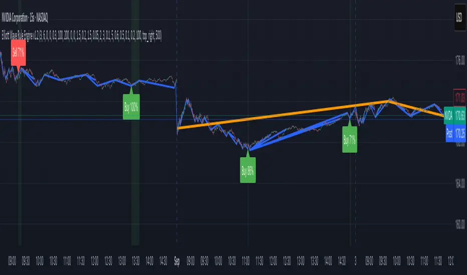
Options Greeks AnalyzerOptions Greeks Analyzer (Training & Learning Guide)
________________________________________
1. Introduction
Options trading is advanced compared to regular stock trading, and one of the most important aspects is Options Greeks. Greeks are mathematical values that measure how the price of an option will react to changes in various factors such as the underlying asset’s price, volatility, interest rates, and time to expiry.
This Options Greeks Analyzer tool is built using TradingView Pine Script v5. It serves as a real time training and analysis dashboard that helps learners visualize how options greeks behave, how option prices change, and how traders can make informed decisions.
📌 Educational Disclaimer:
This tool is only for training and learning purposes. It is not a financial advice tool nor to be used for live trading decisions. The data shown is theoretical Black Scholes model calculations, which may differ from actual option market prices.
________________________________________
2. How the Tool Works
The Options Greeks Analyzer is divided into different modules. Below is a step by step walkthrough:
________________________________________
Step 1: User Inputs
• Implied Volatility (IV%) — You can manually enter volatility, which is the most important factor in option pricing. Higher IV = higher option premium.
• Expiry Selection — Choose from preset durations like 7D, 14D, 30D etc. Days to expiry directly affect time decay (Theta).
• Strike Price Mode — You can select either:
o ATM (At-the-Money = Current price of stock/index)
o Custom strike (Enter your own strike price)
• Risk-Free Rate (%) — A small interest rate factor (like government bond yield) used for theoretical valuation.
• Table Customization — Choose table size, position, and whether to show price lines for easy visibility.
________________________________________
Step 2: Market Data & Volatility
• The tool takes the current market price (Spot Price) as input.
• It calculates realized volatility from historical price fluctuations (using past 30 bars/log returns).
• Implied Volatility (manual input) is then compared to realized vol:
o If IV > Historical Volatility → Market pricing is “expensive” (HIGH IV RANK).
o If IV < Historical Volatility → Market is “cheap” (LOW IV RANK).
o Otherwise, it’s MEDIUM.
📌 Why it matters?
Traders can decide whether buying or selling options is favorable. Beginners learn that timing entry with volatility is more critical than just looking at market direction.
________________________________________
Step 3: Black-Scholes Formula
The core engine uses the Black-Scholes model, a mathematical formula widely used to compute option fair prices.
It uses the following inputs:
• Current price (Spot)
• Strike Price
• Time to Expiry (T)
• Risk Free Rate (r)
• Implied Volatility (σ)
This produces:
• Call Option Price
• Put Option Price
📌 This teaches learners how premiums are derived theoretically and why the same strike can have different values depending on IV and time.
________________________________________
Step 4: Option Greeks Calculation
The tool computes the first order Greeks:
• Delta → Measures how much the option price changes when the underlying stock moves by 1 point.
(Call Delta ranges 0–1, Put Delta ranges -1 to 0).
• Gamma → Sensitivity of Delta to price change. A measure of volatility risk.
• Theta → Time decay. Shows how much value option loses as each day passes. Calls and Puts have negative Theta (decay).
• Vega → Measures how sensitive option price is to volatility changes.
• Rho → Interest rate sensitivity. Mostly minor in equity options but important for training.
📌 New traders learn how each factor impacts profits/losses. Instead of random guessing, they see mathematical impact in numbers.
________________________________________
Step 5: Dashboard & Visualization
The tool builds a professional dashboard table on the chart.
It shows categories such as:
1. Asset Info — Spot, Strike, DTE (days to expiry), IV%, IV Rank, 1-Day Trend, Moneyness (ATM/OTM/ITM).
2. Option Prices — Call, Put, Break-even levels, Time Value, Expected Move (%), Realized vs Implied Vol.
3. Greeks with Visual Progress Bars — Easily shows Delta, Gamma, Vega, Theta, Rho in intuitive graphical representations.
4. Status Bar — Suggests theoretical bias like:
o HIGH IV → Favor Option Selling
o LOW IV → Favor Option Buying
o MEDIUM → Neutral observation
5. Recommendation Line — Offers training-based suggestions like “Buy Straddles”, “Sell Call Spreads”, etc. These are not signals, but scenarios to learn strategies.
________________________________________
3. How It Helps Beginners
1. Learn Greeks in Action:
Beginners often memorize formulas but never see real-time changes. This dashboard updates every bar to show how Greeks change dynamically.
2. Compare Volatilities:
Traders understand difference between historical vs implied volatility and why option premiums behave differently.
3. Understand Risk Levels:
The tool highlights when Gamma risk is high (danger for sellers) or when Theta is most favorable.
4. Training Mode for Strategies:
Helps beginners experiment by changing IV, strike, expiry and seeing how straddles, spreads, naked options would behave theoretically.
5. Prepares Before Live Trading:
Safe environment to practice option analysis without risking capital.
________________________________________
4. Educational Use Cases
• Scenario 1: Change expiry from 7D to 30D — see how Theta becomes slower for longer expiries.
• Scenario 2: Increase IV from 25% to 80% — watch how option premiums inflate, and recommendation changes from “Buy” to “Sell”.
• Scenario 3: Select OTM vs ITM strikes — check how delta moves from near 0 to near 1.
By running these scenarios, learners understand why professional traders hedge Greeks instead of directional gambling.
________________________________________
5. Disclaimer
This Options Greeks Analyzer is built strictly for educational and training purposes.
• It uses theoretical formulas (Black-Scholes) that may not match actual option market prices.
• The recommendations are for learning strategy logic only, not real-world execution signals.
• Trading in options carries significant risks and may result in capital loss.
📌 Always consult with a financial advisor before applying real strategies.
________________________________________
✅ Summary
This Options Greeks Analyzer:
• Teaches how Greeks, IV, and premiums work.
• Provides a real-time interactive dashboard for training.
• Helps beginners practice option scenarios safely.
• Is meant strictly for learning and not live trading execution.
________________________________________
________________________________________
Disclaimer from aiTrendview
This script and its trading signals are provided for training and educational purposes only. They do not constitute financial advice or a guaranteed trading system. Trading involves substantial risk, and there is the potential to lose all invested capital. Users should perform their own analysis and consult with qualified financial professionals before making any trading decisions. aiTrendview disclaims any liability for losses incurred from using this code or trading based on its signals. Use this tool responsibly, and trade only with risk capital.
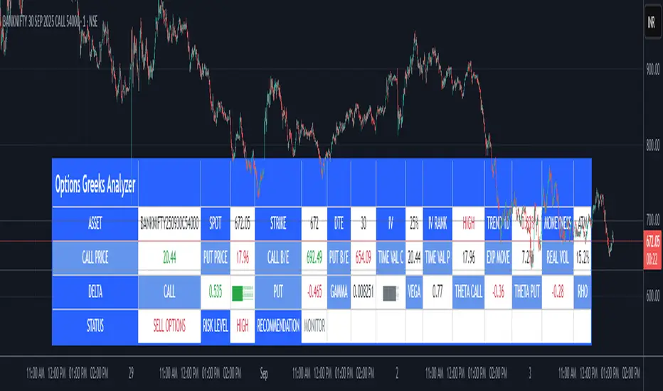
Intrabar Volume Delta — RealTime + History (Stocks/Crypto/Forex)Intrabar Volume Delta Grid — RealTime + History (Stocks/Crypto/Forex)
# Short Description
Shows intrabar Up/Down volume, Delta (absolute/relative) and UpShare% in a compact grid for both real-time and historical bars. Includes an MTF (M1…D1) dashboard, contextual coloring, density controls, and alerts on Δ and UpShare%. Smart historical splitting (“History Mode”) for Crypto/Futures/FX.
---
# What it does (Quick)
* **UpVol / DownVol / Δ / UpShare%** — visualizes order-flow inside each candle.
* **Real-time** — accumulates intrabar volume live by tick-direction.
* **History Mode** — splits Up/Down on closed bars via simple or range-aware logic.
* **MTF Dashboard** — one table view across M1, M5, M15, M30, H1, H4, D1 (Vol, Up/Down, Δ%, Share, Trend).
* **Contextual opacity** — stronger signals appear bolder.
* **Label density** — draw every N-th bar and limit to last X bars for performance.
* **Alerts** — thresholds for |Δ|, Δ%, and UpShare%.
---
# How it works (Real-Time vs History)
* **Real-time (open bar):** volume increments into **UpVolRT** or **DownVolRT** depending on last price move (↑ goes to Up, ↓ to Down). This approximates live order-flow even when full tick history isn’t available.
* **History (closed bars):**
* **None** — no split (Up/Down = 0/0). Safest for equities/indices with unreliable tick history.
* **Approx (Close vs Open)** — all volume goes to candle direction (green → Up 100%, red → Down 100%). Fast but yields many 0/100% bars.
* **Price Action Based** — splits by Close position within High-Low range; strength = |Close−mid|/(High−Low). Above mid → more Up; below mid → more Down. Falls back to direction if High==Low.
* **Auto** — **Stocks/Index → None**, **Crypto/Futures/FX → Approx**. If you see too many 0/100 bars, switch to **Price Action Based**.
---
# Rows & Meaning
* **Volume** — total bar volume (no split).
* **UpVol / DownVol** — directional intrabar volume.
* **Delta (Δ)** — UpVol − DownVol.
* **Absolute**: raw units
* **Relative (Δ%)**: Δ / (Up+Down) × 100
* **Both**: shows both formats
* **UpShare%** — UpVol / (Up+Down) × 100. >50% bullish, <50% bearish.
* Helpful icons: ▲ (>65%), ▼ (<35%).
---
# MTF Dashboard (🔧 Enable Dashboard)
A single table with **Vol, Up, Down, Δ%, Share, Trend (🔼/🔽/⏭️)** for selected timeframes (M1…D1). Great for a fast “panorama” read of flow alignment across horizons.
---
# Inputs (Grouped)
## Display
* Toggle rows: **Volume / Up / Down / Delta / UpShare**
* **Delta Display**: Absolute / Relative / Both
## Realtime & History
* **History Mode**: Auto / None / Approx / Price Action Based
* **Compact Numbers**: 1.2k, 1.25M, 3.4B…
## Theme & UI
* **Theme Mode**: Auto / Light / Dark
* **Row Spacing**: vertical spacing between rows
* **Top Row Y**: moves the whole grid vertically
* **Draw Guide Lines**: faint dotted guides
* **Text Size**: Tiny / Small / Normal / Large
## 🔧 Dashboard Settings
* **Enable Dashboard**
* **📏 Table Text Size**: Tiny…Huge
* **🦓 Zebra Rows**
* **🔲 Table Border**
## ⏰ Timeframes (for Dashboard)
* **M1…D1** toggles
## Contextual Coloring
* **Enable Contextual Coloring**: opacity by signal strength
* **Δ% cap / Share offset cap**: saturation caps
* **Min/Max transparency**: solid vs faint extremes
## Label Density & Size
* **Show every N-th bar**: draw labels only every Nth bar
* **Limit to last X bars**: keep labels only in the most recent X bars
## Colors
* Up / Down / Text / Guide
## Alerts
* **Delta Threshold (abs)** — |Δ| in volume units
* **UpShare > / <** — bullish/bearish thresholds
* **Enable Δ% Alert**, **Δ% > +**, **Δ% < −** — relative delta levels
---
# How to use (Quick Start)
1. Add the indicator to your chart (overlay=false → separate pane).
2. **History Mode**:
* Crypto/Futures/FX → keep **Auto** or switch to **Price Action Based** for richer history.
* Stocks/Index → prefer **None** or **Price Action Based** for safer splits.
3. **Label Density**: start with **Limit to last X bars = 30–150** and **Show every N-th bar = 2–4**.
4. **Contextual Coloring**: keep on to emphasize strong Δ% / Share moves.
5. **Dashboard**: enable and pick only the TFs you actually use.
6. **Alerts**: set thresholds (ideas below).
---
# Alerts (in TradingView)
Add alert → pick this indicator → choose any of:
* **Delta exceeds threshold** (|Δ| > X)
* **UpShare above threshold** (UpShare% > X)
* **UpShare below threshold** (UpShare% < X)
* **Relative Delta above +X%**
* **Relative Delta below −X%**
**Starter thresholds (tune per symbol & TF):**
* **Crypto M1/M5**: Δ% > +25…35 (bullish), Δ% < −25…−35 (bearish)
* **FX (tick volume)**: UpShare > 60–65% or < 40–35%
* **Stocks (liquid)**: set **Absolute Δ** by typical volume scale (e.g., 50k / 100k / 500k)
---
# Notes by Market Type
* **Crypto/Futures**: 24/7 and high liquidity — **Price Action Based** often gives nicer history splits than Approx.
* **Forex (FX)**: TradingView volume is typically **tick volume** (not true exchange volume). Treat Δ/Share as tick-based flow, still very useful intraday.
* **Stocks/Index**: historical tick detail can be limited. **None** or **Price Action Based** is a safer default. If you see too many 0/100% shares, switch away from Approx.
---
# “All Timeframes” accuracy
* Works on **any TF** (M1 → D1/W1).
* **Real-time accuracy** is strong for the open bar (live accumulation).
* **Historical accuracy** depends on your **History Mode** (None = safest, Approx = fastest/simplest, Price Action Based = more nuanced).
* The MTF dashboard uses `request.security` and therefore follows the same logic per TF.
---
# Trade Ideas (Use-Cases)
* **Scalping (M1–M5)**: a spike in Δ% + UpShare>65% + rising total Vol → momentum entries.
* **Intraday (M5–M30–H1)**: when multiple TFs show aligned Δ%/Share (e.g., M5 & M15 bullish), join the trend.
* **Swing (H4–D1)**: persistent Δ% > 0 and UpShare > 55–60% → structural accumulation bias.
---
# Advantages
* **True-feeling live flow** on the open bar.
* **Adaptable history** (three modes) to match data quality.
* **Clean visual layout** with guides, compact numbers, contextual opacity.
* **MTF snapshot** for quick bias read.
* **Performance controls** (last X bars, every N-th bar).
---
# Limitations & Care
* **FX uses tick volume** — interpret Δ/Share accordingly.
* **History Mode is an approximation** — confirm with trend/structure/liquidity context.
* **Illiquid symbols** can produce noisy or contradictory signals.
* **Too many labels** can slow charts → raise N, lower X, or disable guides.
---
# Best Practices (Checklist)
* Crypto/Futures: prefer **Price Action Based** for history.
* Stocks: **None** or **Price Action Based**; be cautious with **Approx**.
* FX: pair Δ% & UpShare% with session context (London/NY) and volatility.
* If labels overlap: tweak **Row Spacing** and **Text Size**.
* In the dashboard, keep only the TFs you actually act on.
* Alerts: start around **Δ% 25–35** for “punchy” moves, then refine per asset.
---
# FAQ
**1) Why do some closed bars show 0%/100% UpShare?**
You’re on **Approx** history mode. Switch to **Price Action Based** for smoother splits.
**2) Δ% looks strong but price doesn’t move — why?**
Δ% is an **order-flow** measure. Price also depends on liquidity pockets, sessions, news, higher-timeframe structure. Use confirmations.
**3) Performance slowdown — what to do?**
Lower **Limit to last X bars** (e.g., 30–100), increase **Show every N-th bar** (2–6), or disable **Draw Guide Lines**.
**4) Dashboard values don’t “match” the grid exactly?**
Dashboard is multi-TF via `request.security` and follows the history logic per TF. Differences are normal.
---
# Short “Store” Marketing Blurb
Intrabar Volume Delta Grid reveals the order-flow inside every candle (Up/Down, Δ, UpShare%) — live and on history. With smart history splitting, an MTF dashboard, contextual emphasis, and flexible alerts, it helps you spot momentum and bias across Crypto, Forex (tick volume), and Stocks. Tidy labels and compact numbers keep the panel readable and fast.
BTC(Sats Stacking) - CDC Action zone filterType: Indicator (Pine v6) • Category: Strategy Tools / DCA • Overlay: Yes
Overview
This indicator simulates fixed-amount Bitcoin DCA (dollar-cost averaging) and lets you apply a CDC Action Zone filter to only buy in specific market conditions. It plots EMA(12/26) lines with a shaded zone (green when fast > slow, red when slow > fast), shows buy markers on the chart when a DCA event actually executes, and displays a concise performance table.
The simulation tracks real invested capital (sum of your buys), not hypothetical equity injections, and reports PnL vs invested capital.
Key features
DCA frequency: Everyday, Every week, or Every month
CDC filter: Buy on all days, only when CDC is Green (trend-up above fast EMA), or only when Red (trend-down below fast EMA)
Execution price: Choose to buy at bar close or next bar open
Capital controls: Fixed DCA amount per event, optional max budget cap
Currency support: Portfolio currency label plus optional FX conversion (by symbol or manual rate)
Chart visuals: Buy markers on candles; EMA(12/26) lines with shaded “action zone”
Metrics table: Invested capital, buys executed, BTC accumulated, average price per BTC (quote), equity (portfolio), PnL% vs invested, and CAGR
How it works
CDC state:
Green = EMA(fast) > EMA(slow) and price ≥ EMA(fast)
Red = EMA(fast) < EMA(slow) and price < EMA(fast)
DCA trigger: Fires on new day/week/month boundaries (timeframe-agnostic).
Buy execution: When a DCA event occurs and passes the CDC filter and budget check, the script spends the fixed amount and adds the corresponding BTC at the chosen execution price.
Inputs (highlights)
Simulation
Symbol (blank = current chart), Buy at close/open, DCA amount, Max total invested
DCA Schedule
Everyday / Every week / Every month
CDC Action Zone
Filter mode (All / Green only / Red only), Price source, Fast/Slow EMA lengths (defaults 12/26)
Currency / Conversion
Portfolio currency label, Convert on/off, By symbol (e.g., OANDA:USDTHB) or Manual rate
Backtest Range
Optional start/end dates
Style
Show EMA lines and zone, colors and opacities, buy marker size and color
Display
Show qty/price labels on buys, show metrics table, number formatting
Metrics
Invested capital: Sum of all DCA spends in your portfolio currency
Equity (portfolio): BTC holdings marked to market and converted back if FX is enabled
PnL % vs invested: (Equity / Invested - 1) × 100
CAGR: Based on elapsed time from first in-range bar to the latest bar
Average price per BTC (quote): Spend in quote currency divided by BTC accumulated
Notes
This is an indicator, not a broker-connected strategy. It simulates buys and displays results without placing orders.
For more realistic fills, use Buy at next bar open.
If your portfolio currency differs from the symbol’s quote currency, enable Convert and supply a conversion symbol or manual rate.
EMA shading is purely visual; the filter logic uses the same EMA definitions.
Attribution & License
Inspired by the DCA idea and community simulations; CDC filtering implemented with standard EMA(12/26) logic.
License: MPL-2.0 (see code header).
Author: MiSuNoJo
Disclaimer
This tool is for research and education only and is not financial advice. Past performance does not guarantee future results. Use at your own risk.

Yelober - Market Internal direction+ Key levelsYelober – Market Internals + Key Levels is a focused intraday trading tool that helps you spot high-probability price direction by anchoring decisions to structure that matters: yesterday’s RTH High/Low, today’s pre-market High/Low, and a fast Value Area/POC from the prior session. Paired with a compact market internals dashboard (NYSE/NASDAQ UVOL vs. DVOL ratios, VOLD slopes, TICK/TICKQ momentum, and optional VIX trend), it gives you a real-time read on breadth so you can choose which direction to trade, when to enter (breaks, retests, or fades at PMH/PML/VAH/VAL/POC), and how to plan exits as internals confirm or deteriorate. On top of these intraday decision benefits, it also allows traders—in a very subtle but powerful way—to keep an eye on the VIX and immediately recognize significant spikes or sharp decreases that should be factored in before entering a trade, or used as a quick signal to modify an existing position. In short: clear levels for the chart, live internals for the context, and a smarter, rules-based path to execution.
# Yelober – Market Internals + Key Levels
*A TradingView indicator for session key levels + real‑time market internals (NYSE/NASDAQ TICK, UVOL/DVOL/VOLD, and VIX).*
**Script name in Pine:** `Yelober - Market Internal direction+ Key levels` (Pine v6)
---
## 1) What this indicator does
**Purpose:** Help intraday traders quickly find high‑probability reaction zones and read market internals momentum without switching charts. It overlays yesterday/today’s **automatic price levels** on your active chart and shows a **market breadth table** that summarizes NYSE/NASDAQ buying pressure and TICK direction, with an optional VIX trend read.
### Key features at a glance
* **Automatic Price Levels (overlay on chart)**
* Yesterday’s High/Low of Day (**yHoD**, **yLoD**)
* Extended Hours High/Low (**yEHH**, **yEHL**) across yesterday AH + today pre‑market
* Today’s Pre‑Market High/Low (**PMH**, **PML**)
* Yesterday’s **Value Area High/Low** (**VAH/VAL**) and **Point of Control (POC)** computed from a volume profile of yesterday’s **regular session**
* Smart de‑duplication:
* Shows **only the higher** of (yEHH vs PMH) and **only the lower** of (yEHL vs PML) to avoid redundant bands
* **Market Breadth Table (on‑chart table)**
* **NYSE ratio** = UVOL/DVOL (signed) with **VOLD slope** from session open
* **NASDAQ ratio** = UVOLQ/DVOLQ (signed) with **VOLDQ slope** from session open
* **TICK** and **TICKQ**: live cumulative ratio and short‑term slope
* **VIX** (optional): current value + slope over a configurable lookback/timeframe
* Color‑coded trends with sensible thresholds and optional normalization
---
## 2) How to use it (trader workflow)
1. **Mark your reaction zones**
* Watch **yHoD/yLoD**, **PMH/PML**, and **VAH/VAL/POC** for first touches, break/retest, and failure tests.
* Expect increased responsiveness when multiple levels cluster (e.g., PMH ≈ VAH ≈ daily pivot).
2. **Read the breadth panel for context**
* **NYSE/NASDAQ ratio** (>1 = more up‑volume than down‑volume; <−1 = down‑dominant). Strong green across both favors long setups; red favors short setups.
* **VOLD slopes** (NYSE & NASDAQ): positive and accelerating → broadening participation; negative → persistent pressure.
* **TICK/TICKQ**: cumulative ratio and **slope arrows** (↗ / ↘ / →). Use the slope to gauge **near‑term thrust or fade**.
* **VIX slope**: rising VIX (red) often coincides with risk‑off; falling VIX (green) with risk‑on.
3. **Confluence = higher confidence**
* Example: Price reclaims **PMH** while **NYSE/NASDAQ ratios** print green and **TICK slopes** point ↗ — consider break‑and‑go; if VIX slope is ↘, that adds risk‑on confidence.
* Example: Price rejects **VAH** while **VOLD slopes** roll negative and VIX ↗ — consider fade/reversal.
4. **Risk management**
* Place stops just beyond key levels tested; if breadth flips, tighten or exit.
> **Timeframes:** Works best on 1–15m charts for intraday. Value Area is computed from **yesterday’s RTH**; choose a smaller calculation timeframe (e.g., 5–15m) for stable profiles.
---
## 3) Inputs & settings (what each option controls)
### Global Style
* **Enable all automatic price levels**: master toggle for yHoD/yLoD, yEHH/yEHL, PMH/PML, VAH/VAL/POC.
* **Line style/width**: applies to all drawn levels.
* **Label size/style** and **label color linking**: use the same color as the line or override with a global label color.
* **Maximum bars lookback**: how far the script scans to build yesterday metrics (performance‑sensitive).
### Value Area / Volume Profile
* **Enable Value Area calculations** *(on by default)*: computes yesterday’s **POC**, **VAH**, **VAL** from a simplified intraday volume profile built from yesterday’s **regular session bars**.
* **Max Volume Profile Points** *(default 50)*: lower values = faster; higher = more precise.
* **Value Area Calculation Timeframe** *(default 15)*: the security timeframe used when collecting yesterday’s highs/lows/volumes.
### Individual Level Toggles & Colors
* **yHoD / yLoD** (yesterday high/low)
* **yEHH / yEHL** (yesterday AH + today pre‑market extremes)
* **PMH / PML** (today pre‑market extremes)
* **VAH / VAL / POC** (yesterday RTH value area + point of control)
### Market Breadth Panel
* **Show NYSE / NASDAQ / VIX**: choose which series to display in the table.
* **Table Position / Size / Background Color**: UI placement and legibility.
* **Slope Averaging Periods** *(default 5)*: number of recent TICK/TICKQ ratio points used in slope calculation.
* **Candles for Rate** *(default 10)* & **Normalize Rate**: VIX slope calculation as % change between `now` and `n` candles ago; normalize divides by `n`.
* **VIX Timeframe**: optionally compute VIX on a higher TF (e.g., 15, 30, 60) for a smoother regime read.
* **Volume Normalization** (NYSE & NASDAQ): display VOLD slopes scaled to `tens/thousands/millions/10th millions` for readable magnitudes; color thresholds adapt to your choice.
---
## 4) Data sources & definitions
* **UVOL/VOLD (NYSE)** and **UVOLQ/DVOLQ/VOLDQ (NASDAQ)** via `request.security()`
* **Ratio** = `UVOL/DVOL` (signed; negative when down‑volume dominates)
* **VOLD slope** ≈ `(VOLD_now − VOLD_open) / bars_since_open`, then normalized per your setting
* **TICK/TICKQ**: cumulative sum of prints this session with **positives vs negatives ratio**, plus a simple linear regression **slope** of the last `N` ratio values
* **VIX**: value and slope across a user‑selected timeframe and lookback
* **Sessions (EST/EDT)**
* **Regular:** 09:30–16:00
* **Pre‑Market:** 04:00–09:30
* **After Hours:** 16:00–20:00
* **Extended‑hours extremes** combine **yesterday AH** + **today PM**
> **Note:** All session checks are done with TradingView’s `time(…,"America/New_York")` context. If your broker’s RTH differs (e.g., futures), adjust expectations accordingly.
---
## 5) How the algorithms work (plain English)
### A) Key Levels
* **Yesterday’s RTH High/Low**: scans yesterday’s bars within 09:30–16:00 and records the extremes + bar indices.
* **Extended Hours**: scans yesterday AH and today PM to get **yEHH/yEHL**. Script shows **either yEHH or PMH** (whichever is **higher**) and **either yEHL or PML** (whichever is **lower**) to avoid duplicate bands stacked together.
* **Value Area & POC (RTH only)**
* Build a coarse volume profile with `Max Volume Profile Points` buckets across the price range formed by yesterday’s RTH bars.
* Distribute each bar’s volume uniformly across the buckets it spans (fast approximation to keep Pine within execution limits).
* **POC** = bucket with max volume. **VA** expands from POC outward until **70%** of cumulative volume is enclosed → yields **VAH/VAL**.
### B) Market Breadth Table
* **NYSE/NASDAQ Ratio**: signed UVOL/DVOL with basic coloring.
* **VOLD Slopes**: from session open to current, normalized to human‑readable units; colors flip green/red based on thresholds that map to your normalization setting (e.g., ±2M for NYSE, ±3.5×10M for NASDAQ).
* **TICK/TICKQ Slope**: linear regression over the last `N` ratio points → **↗ / → / ↘** with the rounded slope value.
* **VIX Slope**: % change between now and `n` candles ago (optionally divided by `n`). Red when rising beyond threshold; green when falling.
---
## 6) Recommended presets
* **Stocks (liquid, intraday)**
* Value Area **ON**, `Max Volume Points` = **40–60**, **Timeframe** = **5–15**
* Breadth: show **NYSE & NASDAQ & VIX**, `Slope periods` = **5–8**, `Candles for rate` = **10–20**, **Normalize VIX** = **ON**
* **Index futures / very high‑volume symbols**
* If you see Pine timeouts, set `Max Volume Points` = **20–40** or temporarily **disable Value Area**.
* Keep breadth panel **ON** (it’s light). Consider **VIX timeframe = 15/30** for regime clarity.
---
## 7) Tips, edge cases & performance
* **Performance:** The volume profile is capped (`maxBarsToProcess ≤ 500` and bucketed) to keep it responsive. If you experience slowdowns, reduce `Max Volume Points`, `Maximum bars lookback`, or disable Value Area.
* **Redundant lines:** The script **intentionally suppresses** PMH/PML when yEHH/yEHL are more extreme, and vice‑versa.
* **Label visibility:** Use `Label style = none` if you only want clean lines and read values from the right‑end labels.
* **Futures/RTH differences:** Value Area is from **yesterday’s RTH** only; for 24h instruments the RTH period may not reflect overnight structure.
* **Session transitions:** PMH/PML tracking stops as soon as RTH starts; values persist as static levels for the session.
---
## 8) Known limitations
* Uses public TradingView symbols: `UVOL`, `VOLD`, `UVOLQ`, `DVOLQ`, `VOLDQ`, `TICK`, `TICKQ`, `VIX`. If your data plan or region limits any symbol, the corresponding table rows may show `na`.
* The VA/POC approximation assumes uniform distribution of each bar’s volume across its high–low. That’s fast but not a tick‑level profile.
* Works best on US equities with standard NY session; alternative sessions may need code changes.
---
## 9) Troubleshooting
* **“Script is too slow / timed out”** → Lower `Max Volume Points`, lower `Maximum bars lookback`, or toggle **OFF** `Enable Value Area calculations` for that instrument.
* **Missing breadth values** → Ensure the symbols above load on your account; try reloading chart or switching timeframes once.
* **Overlapping labels** → Set `Label style = none` or reduce label size.
---
## 10) Version / license / contribution
* **Version:** Initial public release (Pine v6).
* **Author:** © yelober
* **License:** Free for community use and enhancement. Please keep author credit.
* **Contributing:** Open PRs/ideas: presets, alert conditions, multi‑day VA composites, optional mid‑value (`(VAH+VAL)/2`), session filter for futures, and alertable state machine for breadth regime transitions.
---
## 11) Quick start (TL;DR)
1. Add the indicator and **keep default settings**.
2. Trade **reactions** at yHoD/yLoD/PMH/PML/VAH/VAL/POC.
3. Use the **breadth table**: look for **green ratios + ↗ slopes** (risk‑on) or **red ratios + ↘ slopes** (risk‑off). Check **VIX** slope for confirmation.
4. Manage risk around levels; when breadth flips against you, tighten or exit.
---
### Changelog (public)
* **v1.0:** First community release with automatic RTH levels, VA/POC approximation, breadth dashboard (NYSE/NASDAQ/TICK/TICKQ/VIX) with normalization and adaptive color thresholds.
Cnagda Liquidit Trading SystemCnagda Liquidit Trading System helps spot where price is likely to trap traders and reverse, then gives simple, actionable Level to entry, place SL, and take profits with confidence. It blends imbalance zones, trend bias, order blocks, liquidity pools, high-probability fake Signal, and context-aware candle patterns into one clean workflow.
🟩🟥 Imbalance boxes: “Crowd rushed, gaps left”
What it is: Green/red boxes mark fast, one-sided moves where price “skipped” orders—think FVG-like zones that often get revisited.
Why it helps: Price frequently pulls back to “fill” these zones, creating clean retest entries with logical stops.
⏩How to use:
Green box = potential demand retest; Red box = potential supply retest. Enter on pullback into box, not on first impulse. Put stop on far side of box and aim first targets at recent swing points.
↕️ Swing bias (HH/HL vs LH/LL): “Which way is the road?”
What it is: Higher-highs/higher-lows = up-bias; Lower-highs/lower-lows = down-bias. system plots Buy/Sell OB levels aligned with that bias.
Why it helps: Trading with the broader flow reduces “hero trades” against institutions. Bias gives clearer entries and cleaner drawdowns.
⏩How to use:
Up-bias: look for long on Buy OB retests. Down-bias: look for short on Sell OB retests. Wait for a small rejection/engulfing to confirm before triggering.
🧱Order blocks: “Where big players remember”
What it is: last opposite-colored candle before an impulsive move—these zones often hold memory and reaction. system plots these as Buy/Sell OB lines.
Why it helps: Many breakouts pull back to the origin. Good entries often happen on retest, not on the breakout chase.
⏩ How to use:
Let price return into the OB, show wick rejection, and decent volume. Enter with stop beyond OB; define risk-reward before entry.
📊Volume coloring: “How Volume is move?”
What it is: Bar color reflects relative volume; inside bars are black. The dashboard also shows Volume and “Volume vs Prev.”
Why it helps: Patterns without volume often fade; volume validates strength and intent of moves.
⏩ How to use:
Favor entries where imbalance/OB/liquidity-grab coincide with higher volume. If volume is weak, reduce size or skip.
🧲 BSL/SSL liquidity pools: “Fishing for stops”
What it is: Equal highs cluster stops above (BSL); equal lows cluster stops below (SSL). system plots these and highlights the nearest one (“magnet”).
Why it helps: Price often sweeps these pools to trigger stops before reversing. This is a prime trap-reversal location.
⏩ How to use:
Watch nearest BSL/SSL. If price wicks through and closes back inside, anticipate a reversal. Trade reaction, not first poke. When price closes beyond, consider that pool mitigated and move on.
🟢🔴 Advanced liquidity grab: “Catch fakeout”
What it is: Bullish grab = makes a new low beyond a prior low but closes back above it, with a long lower wick, small body, and higher volume. Bearish is mirror. Labeled automatically.
Why it helps: It exposes trap moves (stop hunts) and often precedes true direction.
⏩ How to use:
Best when it aligns with a nearby imbalance/OB and supportive volume. Enter on reversal candle break or on retest. Stop goes beyond sweep wick.
🧠 Smart candlestick patterns (only in right place)
What it is: Engulfing, Hammer, Shooting Star, Hanging Man, Doji (with high volume), Morning/Evening Star, Piercing—but marked “effective” only if context (swing/trend/location) agrees.
Why it helps: same pattern in the wrong place is noise; in the right place, it’s signal.
⏩ How to use:
Location first (BSL/SSL/OB/imbalance), then pattern. Treat pattern as trigger/confirmation—one fresh label shows to keep chart clean.
🧭 Dashboard: “Context in a glance”
⏩ Reversal Level: current swing anchor—expect turns or reactions nearby; great for alerts and planning.
⏩ Volume vs Prev + Volume: Strength meter for signal candle—higher adds conviction.
⏩ Nearest Pool: next “magnet” area—look for sweeps/rejections there.
🧩Step-by-step trading flow (with mindset)
⏩ Set bias: HH/HL = long bias, LH/LL = short bias. Counter-trend only on clean sweeps with strong confirmation.
⏩ Find magnet: Check Nearest Pool (BSL/SSL). Focus attention there; it saves screen time.
⏩ Wait for event: Look for a sweep/grab label, or sharp rejection at pool/OB/imbalance. Avoid FOMO.
⏩ Add confluence: Stack 2–3 of these—imbalance box, OB, contextual pattern, supportive volume.
⏩Plan entry: Bullish: trigger above reversal candle high or take retest of FVG/OB. Stop below sweep wick/zone. Target at least 1:1.5–1:2.
Bearish: mirror above.
⏩Manage smartly: Take partials, move to breakeven or trail thoughtfully. Don’t drag stops inside zone out of emotion.
🎛️ Parameter tuning (to reduce human error)
⏩ swingLen: Smaller = faster but noisier; larger = cleaner but slower. Backtest first, then go live.
⏩ Tolerance (ATR or percent): ATR tolerance adapts to volatility (good for fast markets and lower TFs). Start around 0.15–0.30. In calm markets, try percent 0.05–0.15%.
⏩ minBarsGap: Start with 3–5 so equal highs/lows are truly equal—reduces false pools.
❌Common mistakes → ✅ Better habits
⏩Chasing every breakout → Wait for sweep/rejection, then confirm.
⏩Ignoring volume → Validate strength; cut size or skip on weak volume.
⏩Losing history of pools → If reviewing/backtesting, keep mitigated pools visible (dashed/faded).
⏩Over-tight tolerance/too small swingLen → Increases false signals; backtest to find balance.
📝 checklist (before entry)
⏩ Is there a nearby BSL/SSL and did a sweep/grab happen there?
⏩ Is there a close imbalance/OB that price can retest?
⏩ Do we have an effective pattern plus supportive volume?
⏩Is the stop beyond the wick/zone and RR ≥ 1:1.5?
•?((¯°·._.• 🎀 𝐻𝒶𝓅𝓅𝓎 𝒯𝓇𝒶𝒹𝒾𝓃𝑔 🎀 •._.·°¯((?•

Pivot Matrix & Multi-Timeframe Support-Resistance Analytics________________________________________
📘 Study Material for Pivot Matrix & Multi Timeframe Support-Resistance Analytics
(By aiTrendview — Educational Use Only)
________________________________________
🎯 Introduction
The Pivot Matrix & Multi Timeframe Support-Resistance Analytics indicator is designed to help traders visualize pivot points, support/resistance levels, VWAP, and volume flow analytics all in one place. Rather than giving explicit buy/sell calls, the dashboard provides reference insights so a learner may understand how different technical levels interact in real time.
This document explains its functionality step by step with formulas and usage guides.
________________________________________
1️⃣ Pivot System Logic
Pivot points are classic tools for mapping market support and resistance levels.
✦ How Calculated?
Using the Traditional Method:
• Pivot Point (PP):
PP=Highprev+Lowprev+Closeprev3PP = \frac{High_{prev} + Low_{prev} + Close_{prev}}{3}PP=3Highprev+Lowprev+Closeprev
• First Support/Resistance:
R1=2×PP−Lowprev,S1=2×PP−HighprevR1 = 2 \times PP - Low_{prev}, \quad S1 = 2 \times PP - High_{prev}R1=2×PP−Lowprev,S1=2×PP−Highprev
• Second Support/Resistance:
R2=PP+(Highprev−Lowprev),S2=PP−(Highprev−Lowprev)R2 = PP + (High_{prev} - Low_{prev}), \quad S2 = PP - (High_{prev} - Low_{prev})R2=PP+(Highprev−Lowprev),S2=PP−(Highprev−Lowprev)
• Third Levels:
R3=Highprev+2×(PP−Lowprev),S3=Lowprev−2×(Highprev−PP)R3 = High_{prev} + 2 \times (PP - Low_{prev}), \quad S3 = Low_{prev} - 2 \times (High_{prev} - PP)R3=Highprev+2×(PP−Lowprev),S3=Lowprev−2×(Highprev−PP)
• Similarly, R4/R5 and S4/S5 are extrapolated from extended range multipliers.
✦ How Used?
• Price above PP → bullish control bias.
• Price below PP → bearish control bias.
• R1–R5 levels act as resistances; S1–S5 act as supports.
Learners should watch how candles behave when approaching R/S zones to spot breakout vs. rejection conditions.
________________________________________
2️⃣ Multi Timeframe Logic
The indicator allows using daily-based pivot values (via request.security). This ensures alignment with institutional daily levels, not just intraday recalculations.
✦ Teaching Value
Understanding MTF pivots shows how markets respect higher timeframe levels (daily > intraday, weekly > daily). This helps learners grasp nested support-resistance structures.
________________________________________
3️⃣ VWAP (Volume Weighted Average Price)
Formula:
VWAPt=∑(Pricei×Volumei)∑(Volumei),Pricei=High+Low+Close3VWAP_t = \frac{\sum (Price_i \times Volume_i)}{\sum (Volume_i)}, \quad Price_i = \frac{High + Low + Close}{3}VWAPt=∑(Volumei)∑(Pricei×Volumei),Pricei=3High+Low+Close
Usage:
• VWAP is used as an institutional benchmark of fair value.
• Above VWAP = bullish flow.
• Below VWAP = bearish flow.
Learners should check whether price respects VWAP as a magnet or uses it as support/resistance.
________________________________________
4️⃣ Volume Flow Analysis
The script classifies buy volume, sell volume, and neutral volume.
• Buy Volume = if close > open.
• Sell Volume = if close < open.
• Neutral Volume = if close = open.
For daily tracking:
Buy%=DayBuyVolDayTotalVol×100,Sell%=DaySellVolDayTotalVol×100Buy\% = \frac{DayBuyVol}{DayTotalVol} \times 100, \quad Sell\% = \frac{DaySellVol}{DayTotalVol} \times 100Buy%=DayTotalVolDayBuyVol×100,Sell%=DayTotalVolDaySellVol×100
Usage for Learners:
• Dominant Buy% → accumulation/ bullish pressure.
• Dominant Sell% → distribution/ bearish pressure.
• Balanced → sideways liquidity building.
This teaches observation of order flow bias rather than relying only on price.
________________________________________
5️⃣ Dashboard Progress Bars & Colors
The script uses visual progress bars and dynamic colors for clarity. For example:
• VWAP Backgrounds: Green shades when price strongly above VWAP, Red when below.
• Volume Bars: More green blocks mean buying dominance, red means selling pressure.
This visual design turns concepts into easy-to-digest cues, useful for training.
________________________________________
6️⃣ Market Status Summary
Finally, the dashboard synthesizes all data points:
• Price vs Pivot (above or below).
• Price vs VWAP (above or below).
• Volume Pressure (buy side vs sell side).
Status Rule:
• If all three align bullish → Status box turns green.
• If mixed → Neutral grey.
• If bearish dominance → weaker tone.
Why Important?
This teaches learners that market conditions should align in confluence across indicators before confidence arises.
________________________________________
⚠️ Strict Disclaimer (aiTrendview)
The Pivot Matrix & Multi Timeframe Support-Resistance Analytics tool is developed by aiTrendview for strictly educational and research purposes.
❌ It does NOT provide buy/sell recommendations.
❌ It does NOT guarantee profits.
❌ Unauthorized use, copying, or redistribution of this code is prohibited.
⚠️ Trading Risk Warning:
• Trading involves high risk of financial loss.
• You may lose more than your capital.
• Past levels and indicators do not predict future outcomes.
This tool must be viewed as a visual education aid to practice technical analysis skills, not as trading advice.
________________________________________
✅ Now you have a step by step study guide:
• Pivot calculations explained
• VWAP with logic
• Volume breakdown
• Visual analytics
• Status confluence logic
• Disclaimer for compliance
________________________________________
⚠️ Warning:
• Trading financial markets involves substantial risk.
• You can lose more money than you invest.
• Past performance of indicators does not guarantee future results.
• This script must not be copied, resold, or republished without authorization from aiTrendview.
By using this material or the code, you agree to take full responsibility for your trading decisions and acknowledge that this is not financial advice.
________________________________________
⚠️ Disclaimer and Warning (From aiTrendview)
This Dynamic Trading Dashboard is created strictly for educational and research purposes on the TradingView platform. It does not provide financial advice, buy/sell recommendations, or guaranteed returns. Any use of this tool in live trading is completely at the user’s own risk. Markets are inherently risky; losses can exceed initial investment.
The intellectual property of this script and its methodology belongs to aiTrendview. Unauthorized reproduction, modification, or redistribution of this code is strictly prohibited. By using this study material or the script, you acknowledge personal responsibility for any trading outcomes. Always consult professional financial advisors before making investment decisions.

FUMO 200 MagnetWhat it does
FUMO Magnet measures how far price has stretched away from its long-term “magnet” — a blended EMA/SMA moving average (200 by default).
It plots a logarithmic deviation (optionally normalized) as an oscillator around zero.
Above 0** → price is above the magnet (stretched up)
Below 0** → price is below the magnet (stretched down)
Guide levels** highlight potential overbought/oversold zones
---
Why log deviation?
Log returns make extremes comparable across cycles and compress exponential trends — especially useful for BTC and other crypto assets.
Normalization modes further adjust the scale, keeping the oscillator readable on any chart.
---
Inputs
**Base**
* Source (default: Close)
* Base Length (default: 200 EMA/SMA)
* EMA vs SMA weight (%) — 0% = pure SMA, 100% = pure EMA, 50% = blended
* EMA smoothing of deviation — acts as a noise filter
**Normalization**
* None (Log Deviation) — raw log stretch in % terms
* Z-score — deviation in standard deviations (σ)
* Robust Z (MAD) — deviation vs median absolute deviation, resistant to outliers
* Tanh squash — smooth nonlinear squash of extremes for compact scale
* Normalization window (for Z / MAD)
* Tanh scale (lower = stronger squash)
* Clamp after normalization — hard cap at ±X
**Levels**
* Guide levels (Upper / Lower) — visual thresholds (default ±12)
* Zero line toggle
---
### How to read it
* **Trend bias**: sustained time above 0 = uptrend, below 0 = downtrend
* **Stretch / mean reversion**: the farther from 0, the higher the reversion risk
* **Cross-checks**: combine with structure (HH/HL, LH/LL), volume, or momentum (RSI, MACD)
---
### Recommended settings by timeframe
**Long-term (1D / 1W)**
* Normalization: None (Log Deviation)
* Base Length: 200
* EMA vs SMA weight: 50% (adjust 35–65% for faster/slower magnet)
* Deviation smoothing: 20 (10–30 range)
* Guide levels: ±12 to ±20
* Use case: cycle extremes, portfolio rebalancing, trim/add logic
**Swing (4H – 1D)**
* Normalization: Z-score
* Window: 200 (100–250)
* Smoothing: 14–20
* Guide levels: ±2σ to ±3σ
* Use case: stretched conditions across regimes; ±3σ is rare, often mean-reverts
**Intraday / Active swing (1H – 4H)**
* Normalization: Robust Z (MAD)
* Window: 200 (150 for faster response)
* Smoothing: 10–16
* Guide levels: ±3 to ±4 (robust units)
* Use case: handles spikes better than σ, fewer false overbought/oversold signals
**Scalping / Universal readability (15m – 1H)**
* Normalization: Tanh squash
* Tanh scale: 6–10 (start with 8)
* Smoothing: 8–12
* Guide levels: ±8 to ±12
* Use case: compact panel across assets and timeframes; not % or σ, but visually consistent
---
### Optional
* Clamp: enable ±20 (or ±25) for strict bounded range (useful for public charts)
---
### Quick setups
**BTC Daily (“cycle view”)**
* Normalization: None
* Blend: 50%
* Smooth: 20
* Levels: ±12–15
**BTC 4H (“swing”)**
* Normalization: Z-score
* Window: 200
* Smooth: 16
* Levels: ±2.5σ to ±3σ
**Alts 1H (“volatile”)**
* Normalization: Robust Z (MAD)
* Window: 200
* Smooth: 12
* Levels: ±3.5 to ±4.5
**Mixed assets 15m (“compact panel”)**
* Normalization: Tanh squash
* Scale: 8
* Smooth: 10
* Levels: ±8–12
* Clamp: ±20
Advanced Volume Profile Pro Delta + POC + VAH/VAL# Advanced Volume Profile Pro - Delta + POC + VAH/VAL Analysis System
## WHAT THIS SCRIPT DOES
This script creates a comprehensive volume profile analysis system that combines traditional volume-at-price distribution with delta volume calculations, Point of Control (POC) identification, and Value Area (VAH/VAL) analysis. Unlike standard volume indicators that show only total volume over time, this script analyzes volume distribution across price levels and estimates buying vs selling pressure using multiple calculation methods to provide deeper market structure insights.
## WHY THIS COMBINATION IS ORIGINAL AND USEFUL
**The Problem Solved:** Traditional volume indicators show when volume occurs but not where price finds acceptance or rejection. Standalone volume profiles lack directional bias information, while basic delta calculations don't provide structural context. Traders need to understand both volume distribution AND directional sentiment at key price levels.
**The Solution:** This script implements an integrated approach that:
- Maps volume distribution across price levels using configurable row density
- Estimates delta (buying vs selling pressure) using three different methodologies
- Identifies Point of Control (highest volume price level) for key support/resistance
- Calculates Value Area boundaries where 70% of volume traded
- Provides real-time alerts for key level interactions and volume imbalances
**Unique Features:**
1. **Developing POC Visualization**: Real-time tracking of Point of Control migration throughout the session via blue dotted trail, revealing institutional accumulation/distribution patterns before they complete
2. **Multi-Method Delta Calculation**: Price Action-based, Bid/Ask estimation, and Cumulative methods for different market conditions
3. **Adaptive Timeframe System**: Auto-adjusts calculation parameters based on chart timeframe for optimal performance
4. **Flexible Profile Types**: N Bars Back (precise control), Days Back (calendar-based), and Session-based analysis modes
5. **Advanced Imbalance Detection**: Identifies and highlights significant buying/selling imbalances with configurable thresholds
6. **Comprehensive Alert System**: Monitors POC touches, Value Area entry/exit, and major volume imbalances
## HOW THE SCRIPT WORKS TECHNICALLY
### Core Volume Profile Methodology:
**1. Price Level Distribution:**
- Divides price range into user-defined rows (10-50 configurable)
- Calculates row height: `(Highest Price - Lowest Price) / Number of Rows`
- Distributes each bar's volume across price levels it touched proportionally
**2. Delta Volume Calculation Methods:**
**Price Action Method:**
```
Price Range = High - Low
Buy Pressure = (Close - Low) / Price Range
Sell Pressure = (High - Close) / Price Range
Buy Volume = Total Volume × Buy Pressure
Sell Volume = Total Volume × Sell Pressure
Delta = Buy Volume - Sell Volume
```
**Bid/Ask Estimation Method:**
```
Average Price = (High + Low + Close) / 3
Buy Volume = Close > Average ? Volume × 0.6 : Volume × 0.4
Sell Volume = Total Volume - Buy Volume
```
**Cumulative Method:**
```
Buy Volume = Close > Open ? Volume : Volume × 0.3
Sell Volume = Close ≤ Open ? Volume : Volume × 0.3
```
**3. Point of Control (POC) Identification:**
- Scans all price levels to find maximum volume concentration
- POC represents the price level with highest trading activity
- Acts as significant support/resistance level
- **Developing POC Feature**: Tracks POC evolution in real-time via blue dotted trail, showing how institutional interest migrates throughout the session. Upward POC migration indicates accumulation patterns, downward migration suggests distribution, providing early trend signals before price confirmation.
**4. Value Area Calculation:**
- Starts from POC and expands up/down to encompass 70% of total volume
- VAH (Value Area High): Upper boundary of value area
- VAL (Value Area Low): Lower boundary of value area
- Expansion algorithm prioritizes direction with higher volume
**5. Adaptive Range Selection:**
Based on profile type and timeframe optimization:
- **N Bars Back**: Fixed lookback period with performance optimization (20-500 bars)
- **Days Back**: Calendar-based analysis with automatic timeframe adjustment (1-365 days)
- **Session**: Current trading session or custom session times
### Performance Optimization Features:
- **Sampling Algorithm**: Reduces calculation load on large datasets while maintaining accuracy
- **Memory Management**: Clears previous drawings to prevent performance degradation
- **Safety Constraints**: Prevents excessive memory usage with configurable limits
## HOW TO USE THIS SCRIPT
### Initial Setup:
1. **Profile Configuration**: Select profile type based on trading style:
- N Bars Back: Precise control over data range
- Days Back: Intuitive calendar-based analysis
- Session: Real-time session development
2. **Row Density**: Set number of rows (30 default) - more rows = higher resolution, slower performance
3. **Delta Method**: Choose calculation method based on market type:
- Price Action: Best for trending markets
- Bid/Ask Estimate: Good for ranging markets
- Cumulative: Smoothed approach for volatile markets
4. **Visual Settings**: Configure colors, position (left/right), and display options
### Reading the Profile:
**Volume Bars:**
- **Length**: Represents relative volume at that price level
- **Color**: Green = net buying pressure, Red = net selling pressure
- **Intensity**: Darker colors indicate volume imbalances above threshold
**Key Levels:**
- **POC (Blue Line)**: Highest volume price - major support/resistance
- **VAH (Purple Dashed)**: Value Area High - upper boundary of fair value
- **VAL (Orange Dashed)**: Value Area Low - lower boundary of fair value
- **Value Area Fill**: Shaded region showing main trading range
**Developing POC Trail:**
- **Blue Dotted Lines**: Show real-time POC evolution throughout the session
- **Migration Patterns**: Upward trail indicates bullish accumulation, downward trail suggests bearish distribution
- **Early Signals**: POC movement often precedes price movement, providing advance warning of institutional activity
- **Institutional Footprints**: Reveals where smart money concentrated volume before final POC establishment
### Trading Applications:
**Support/Resistance Analysis:**
- POC acts as magnetic price level - expect reactions
- VAH/VAL provide intermediate support/resistance levels
- Profile edges show areas of low volume acceptance
**Developing POC Analysis:**
- **Upward Migration**: POC moving higher = institutional accumulation, bullish bias
- **Downward Migration**: POC moving lower = institutional distribution, bearish bias
- **Stable POC**: Tight clustering = balanced market, range-bound conditions
- **Early Trend Detection**: POC direction change often precedes price breakouts
**Entry Strategies:**
- Buy at VAL with POC as target (in uptrends)
- Sell at VAH with POC as target (in downtrends)
- Breakout plays above/below profile extremes
**Volume Imbalance Trading:**
- Strong buying imbalance (>60% threshold) suggests continued upward pressure
- Strong selling imbalance suggests continued downward pressure
- Imbalances near key levels provide high-probability setups
**Multi-Timeframe Context:**
- Use higher timeframe profiles for major levels
- Lower timeframe profiles for precise entries
- Session profiles for intraday trading structure
## SCRIPT SETTINGS EXPLANATION
### Volume Profile Settings:
- **Profile Type**: Determines data range for calculation
- N Bars Back: Exact number of bars (20-500 range)
- Days Back: Calendar days with timeframe adaptation (1-365 days)
- Session: Trading session-based (intraday focus)
- **Number of Rows**: Profile resolution (10-50 range)
- **Profile Width**: Visual width as chart percentage (10-50%)
- **Value Area %**: Volume percentage for VA calculation (50-90%, 70% standard)
- **Auto-Adjust**: Automatically optimizes for different timeframes
### Delta Volume Settings:
- **Show Delta Volume**: Enable/disable delta calculations
- **Delta Calculation Method**: Choose methodology based on market conditions
- **Highlight Imbalances**: Visual emphasis for significant volume imbalances
- **Imbalance Threshold**: Percentage for imbalance detection (50-90%)
### Session Settings:
- **Session Type**: Daily, Weekly, Monthly, or Custom periods
- **Custom Session Time**: Define specific trading hours
- **Previous Sessions**: Number of historical sessions to display
### Days Back Settings:
- **Lookback Days**: Number of calendar days to analyze (1-365)
- **Automatic Calculation**: Script automatically converts days to bars based on timeframe:
- Intraday: Accounts for 6.5 trading hours per day
- Daily: 1 bar per day
- Weekly/Monthly: Proportional adjustment
### N Bars Back Settings:
- **Lookback Bars**: Exact number of bars to analyze (20-500)
- **Precise Control**: Best for systematic analysis and backtesting
### Visual Customization:
- **Colors**: Bullish (green), Bearish (red), and level colors
- **Profile Position**: Left or Right side of chart
- **Profile Offset**: Distance from current price action
- **Labels**: Show/hide level labels and values
- **Smooth Profile Bars**: Enhanced visual appearance
### Alert Configuration:
- **POC Touch**: Alerts when price interacts with Point of Control
- **VA Entry/Exit**: Alerts for Value Area boundary interactions
- **Major Imbalance**: Alerts for significant volume imbalances
## VISUAL FEATURES
### Profile Display:
- **Horizontal Bars**: Volume distribution across price levels
- **Color Coding**: Delta-based coloring for directional bias
- **Smooth Rendering**: Optional smoothing for cleaner appearance
- **Transparency**: Configurable opacity for chart readability
### Level Lines:
- **POC**: Solid blue line with optional label
- **VAH/VAL**: Dashed colored lines with value displays
- **Extension**: Lines extend across relevant time periods
- **Value Area Fill**: Optional shaded region between VAH/VAL
### Information Table:
- **Current Values**: Real-time POC, VAH, VAL prices
- **VA Range**: Value Area width calculation
- **Positioning**: Multiple table positions available
- **Text Sizing**: Adjustable for different screen sizes
## IMPORTANT USAGE NOTES
**Realistic Expectations:**
- Volume profile analysis provides structural context, not trading signals
- Delta calculations are estimations based on price action, not actual order flow
- Past volume distribution does not guarantee future price behavior
- Combine with other analysis methods for comprehensive market view
**Best Practices:**
- Use appropriate profile types for your trading style:
- Day Trading: Session or Days Back (1-5 days)
- Swing Trading: Days Back (10-30 days) or N Bars Back
- Position Trading: Days Back (60-180 days)
- Consider market context (trending vs ranging conditions)
- Verify key levels with additional technical analysis
- Monitor profile development for changing market structure
**Performance Considerations:**
- Higher row counts increase calculation complexity
- Large lookback periods may affect chart performance
- Auto-adjust feature optimizes for most use cases
- Consider using session profiles for intraday efficiency
**Limitations:**
- Delta calculations are estimations, not actual transaction data
- Profile accuracy depends on available price/volume history
- Effectiveness varies across different instruments and market conditions
- Requires understanding of volume profile concepts for optimal use
**Data Requirements:**
- Requires volume data for accurate calculations
- Works best on liquid instruments with consistent volume
- May be less effective on very low volume or exotic instruments
This script serves as a comprehensive volume analysis tool for traders who need detailed market structure information with integrated directional bias analysis and real-time POC development tracking for informed trading decisions.