Wavelet Filter with Adaptive Upsampling [BackQuant]Wavelet Filter with Adaptive Upsampling
The Wavelet Filter with Adaptive Upsampling is an advanced filtering and signal reconstruction tool designed to enhance the analysis of financial time series data. It combines wavelet transforms with adaptive upsampling techniques to filter and reconstruct price data, making it ideal for capturing subtle market movements and enhancing trend detection. This system uses high-pass and low-pass filters to decompose the price series into different frequency components, applying adaptive thresholding to eliminate noise and preserve relevant signal information.
Shout out to Loxx for the Least Squares fitting of trigonometric series and Quinn and Fernandes algorithm for finding frequency
www.tradingview.com
Key Features
1. Frequency Decomposition with High-Pass and Low-Pass Filters:
The indicator decomposes the input time series using high-pass and low-pass filters to separate the high-frequency (detail) and low-frequency (trend) components of the data. This decomposition allows for a more accurate analysis of underlying trends, while mitigating the impact of noise.
2. Soft Thresholding for Noise Reduction:
A soft thresholding function is applied to the high-frequency component, allowing for the reduction of noise while retaining significant market signals. This function adjusts the coefficients of the high-frequency data, removing small fluctuations and leaving only the essential price movements.
3. Adaptive Upsampling Process:
The upsampling process in this script can be customized using different methods: sinusoidal upsampling, advanced upsampling, and simple upsampling. Each method serves a unique purpose:
Sinusoidal Upsample uses a sine wave to interpolate between data points, providing a smooth transition.
Advanced Upsample utilizes a Quinn-Fernandes algorithm to estimate frequency and apply more sophisticated interpolation techniques, adapting to the market’s cyclical behavior.
Simple Upsample linearly interpolates between data points, providing a basic upsampling technique for less complex analysis.
4. Reconstruction of Filtered Signal:
The indicator reconstructs the filtered signal by summing the high and low-frequency components after upsampling. This allows for a detailed yet smooth representation of the original time series, which can be used for analyzing underlying trends in the market.
5. Visualization of Reconstructed Data:
The reconstructed series is plotted, showing how the upsampling and filtering process enhances the clarity of the price movements. Additionally, the script provides the option to visualize the log returns of the reconstructed series as a histogram, with positive returns shown in green and negative returns in red.
6. Cumulative Series and Trend Detection:
A cumulative series is plotted to visualize the compounded effect of the filtered and reconstructed data. This feature helps traders track the overall performance of the asset over time, identifying whether the asset is following a sustained upward or downward trend.
7. Adaptive Thresholding and Noise Estimation:
The system estimates the noise level in the high-frequency component and applies an adaptive thresholding process based on the standard deviation of the downsampled data. This ensures that only significant price movements are retained, further refining the trend analysis.
8. Customizable Parameters for Flexibility:
Users can customize the following parameters to adjust the behavior of the indicator:
Frequency and Phase Shift: Control the periodicity of the wavelet transformation and the phase of the upsampling function.
Upsample Factor: Adjust the level of interpolation applied during the upsampling process.
Smoothing Period: Determine the length of time used to smooth the signal, helping to filter out short-term fluctuations.
References
Enhancing Cross-Sectional Currency Strategies with Context-Aware Learning to Rank
arxiv.org
Daubechies Wavelet - Wikipedia
en.wikipedia.org
Quinn Fernandes Fourier Transform of Filtered Price by Loxx
Note on Usage for Mean-Reversion Strategy
This indicator is primarily designed for trend-following strategies. However, by taking the inverse of the signals, it can be adapted for mean-reversion strategies. This involves buying underperforming assets and selling outperforming ones. Caution: This method may not work effectively with highly correlated assets, as the price movements between correlated assets tend to mirror each other, limiting the effectiveness of mean-reversion strategies.
Final Thoughts
The Wavelet Filter with Adaptive Upsampling is a powerful tool for traders seeking to improve their understanding of market trends and noise. By using advanced wavelet decomposition and adaptive upsampling, this system offers a clearer, more refined picture of price movements, enhancing trend-following strategies. It’s particularly useful for detecting subtle shifts in market momentum and reconstructing price data in a way that removes noise, providing more accurate insights into market conditions.
在腳本中搜尋"长江电子+半导体行业研究框架培训+pdf"

ErrorFunctionsLibrary "ErrorFunctions"
A collection of functions used to approximate the area beneath a Gaussian curve.
Because an ERF (Error Function) is an integral, there is no closed-form solution to calculating the area beneath the curve. Meaning all ERFs are approximations; precisely wrong, but mostly accurate. How close you need to get to the actual area depends entirely on your use case, with more precision being less efficient.
The internal precision of floats in Pine Script is 1e-16 (16 decimals, aka. double precision). This library adapts well known algorithms designed to efficiently reach double precision. Single precision alternates are also included. All of them were made free to use, modify, and distribute by their original authors.
HASTINGS
Adaptation of a single precision ERF by Cecil Hastings Jr, published through Princeton University in 1955. It was later documented by Abramowitz and Stegun as equation 7.1.26 in their 1972 Handbook of Mathematical Functions. Fast, efficient, and ideal when precision beyond a few decimals is unnecessary.
GILES
Adaptation of a single precision Inverse ERF by Michael Giles, published through the University of Oxford in 2012. It reverses the ERF, estimating an X coordinate from an area. It too is fast, efficient, and ideal when precision beyond a few decimals is unnecessary.
LIBC
Adaptation of the double precision ERF & ERFC in the standard C library (aka. libc). It is also the same ERF & ERFC that SciPy uses. While not quite as efficient as the Hastings approximation, it's still very fast and fully maximizes Pines precision.
BOOST
Adaptation of the double precision Inverse ERF & Inverse ERFC in the Boost Math C++ library. SciPy uses these as well. These reverse the ERF & ERFC, estimating an X coordinate from an area. It too isn't quite as efficient as the Giles approximation, but still fast and fully maximizes Pines precision.
While these algorithms are not exported directly, they are available through their exported counterparts.
- - -
ERROR FUNCTIONS
erf(x, precise)
An Error Function estimates the theoretical error of a measurement.
Parameters:
x (float) : (float) Upper limit of the integration.
precise (bool) : Double precision (true) or single precision (false).
Returns: (float) Between -1 and 1.
erfc(x, precise)
A Complementary Error Function estimates the difference between a theoretical error and infinity.
Parameters:
x (float) : (float) Lower limit of the integration.
precise (bool) : Double precision (true) or single precision (false).
Returns: (float) Between 0 and 2.
erfinv(x, precise)
An Inverse Error Function reverses the erf() by estimating the original measurement from the theoretical error.
Parameters:
x (float) : (float) Theoretical error.
precise (bool) : Double precision (true) or single precision (false).
Returns: (float) Between 0 and ± infinity.
erfcinv(x, precise)
An Inverse Complementary Error Function reverses the erfc() by estimating the original measurement from the difference between the theoretical error and infinity.
Parameters:
x (float) : (float) Difference between the theoretical error and infinity.
precise (bool) : Double precision (true) or single precision (false).
Returns: (float) Between 0 and ± infinity.
- - -
DISTRIBUTION FUNCTIONS
pdf(x, m, s)
A Probability Density Function estimates the probability density . For clarity, density is not a probability .
Parameters:
x (float) : (float) X coordinate for which a density will be estimated.
m (float) : (float) Mean
s (float) : (float) Sigma
Returns: (float) Between 0 and ∞.
cdf(z, precise)
A Cumulative Distribution Function estimates the area under a Gaussian curve between negative infinity and the Z Score.
Parameters:
z (float) : (float) Z Score.
precise (bool) : Double precision (true) or single precision (false).
Returns: (float) Between 0 and 1.
cdfinv(a, precise)
An Inverse Cumulative Distribution Function reverses the cdf() by estimating the Z Score from an area.
Parameters:
a (float) : (float) Area between 0 and 1.
precise (bool) : Double precision (true) or single precision (false).
Returns: (float) Between -∞ and +∞
cdfab(z1, z2, precise)
A Cumulative Distribution Function from A to B estimates the area under a Gaussian curve between two Z Scores (A and B).
Parameters:
z1 (float) : (float) First Z Score.
z2 (float) : (float) Second Z Score.
precise (bool) : Double precision (true) or single precision (false).
Returns: (float) Between 0 and 1.
ttt(z, precise)
A Two-Tailed Test estimates the area under a Gaussian curve between symmetrical ± Z scores and ± infinity.
Parameters:
z (float) : (float) One of the symmetrical Z Scores.
precise (bool) : Double precision (true) or single precision (false).
Returns: (float) Between 0 and 1.
tttinv(a, precise)
An Inverse Two-Tailed Test reverses the ttt() by estimating the absolute Z Score from an area.
Parameters:
a (float) : (float) Area between 0 and 1.
precise (bool) : Double precision (true) or single precision (false).
Returns: (float) Between 0 and ∞.
ott(z, precise)
A One-Tailed Test estimates the area under a Gaussian curve between an absolute Z Score and infinity.
Parameters:
z (float) : (float) Z Score.
precise (bool) : Double precision (true) or single precision (false).
Returns: (float) Between 0 and 1.
ottinv(a, precise)
An Inverse One-Tailed Test Reverses the ott() by estimating the Z Score from a an area.
Parameters:
a (float) : (float) Area between 0 and 1.
precise (bool) : Double precision (true) or single precision (false).
Returns: (float) Between 0 and ∞.

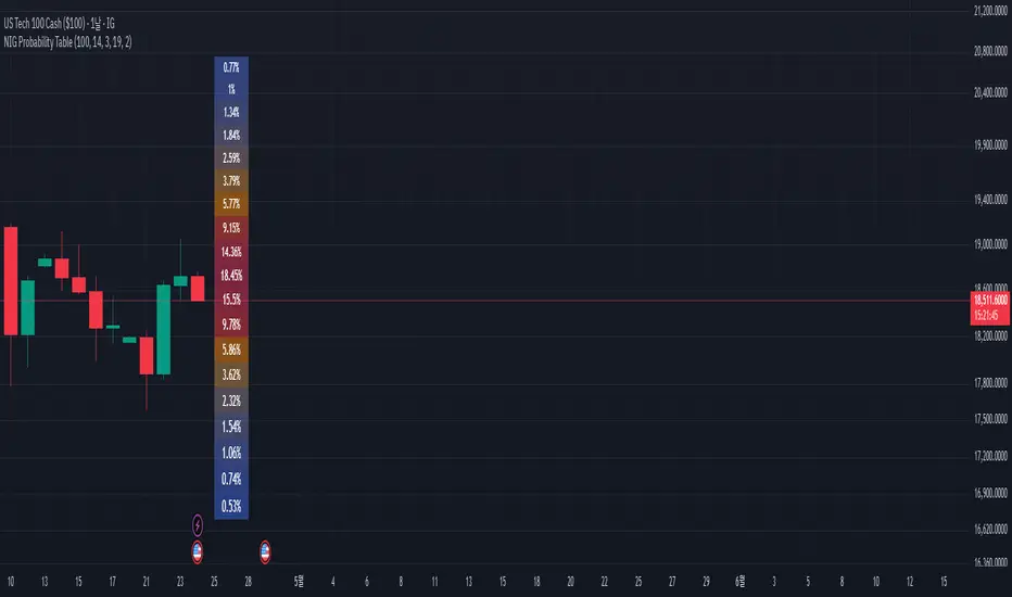
NIG Probability TableNormal-Inverse Gaussian Probability Table
This indicator implements the Normal-Inverse Gaussian (NIG) distribution to estimate the likelihood of future price based on recent market behavior.
📊 Key Features:
- Estimates the parameters (α: tail heaviness, β: skewness, δ: scale, μ: location)
of the NIG distribution using a sliding window over log returns.
- Uses a numerically approximated version of the modified Bessel function (K₁)
to calculate the NIG probability density function (PDF).
- Normalizes the total probability across all bins to ensure the values are interpretable.
- Displays a dynamic probability table showing the chance of future returns falling into each bin.
⚠️ Notes:
- This is a real-time approximation. The Bessel function and posterior inference are simplified.
- Tail probabilities and shape parameters are sensitive to the window size and input settings.
- Useful for risk analysis, option overlays, and strategy filters.
Stochastic Order Flow Momentum [ScorsoneEnterprises]This indicator implements a stochastic model of order flow using the Ornstein-Uhlenbeck (OU) process, combined with a Kalman filter to smooth momentum signals. It is designed to capture the dynamic momentum of volume delta, representing the net buying or selling pressure per bar, and highlight potential shifts in market direction. The volume delta data is sourced from TradingView’s built-in functionality:
www.tradingview.com
For a deeper dive into stochastic processes like the Ornstein-Uhlenbeck model in financial contexts, see these research articles: arxiv.org and arxiv.org
The SOFM tool aims to reveal the momentum and acceleration of order flow, modeled as a mean-reverting stochastic process. In markets, order flow often oscillates around a baseline, with bursts of buying or selling pressure that eventually fade—similar to how physical systems return to equilibrium. The OU process captures this behavior, while the Kalman filter refines the signal by filtering noise. Parameters theta (mean reversion rate), mu (mean level), and sigma (volatility) are estimated by minimizing a squared-error objective function using gradient descent, ensuring adaptability to real-time market conditions.
How It Works
The script combines a stochastic model with signal processing. Here’s a breakdown of the key components, including the OU equation and supporting functions.
// Ornstein-Uhlenbeck model for volume delta
ou_model(params, v_t, lkb) =>
theta = clamp(array.get(params, 0), 0.01, 1.0)
mu = clamp(array.get(params, 1), -100.0, 100.0)
sigma = clamp(array.get(params, 2), 0.01, 100.0)
error = 0.0
v_pred = array.new(lkb, 0.0)
array.set(v_pred, 0, array.get(v_t, 0))
for i = 1 to lkb - 1
v_prev = array.get(v_pred, i - 1)
v_curr = array.get(v_t, i)
// Discretized OU: v_t = v_{t-1} + theta * (mu - v_{t-1}) + sigma * noise
v_next = v_prev + theta * (mu - v_prev)
array.set(v_pred, i, v_next)
v_curr_clean = na(v_curr) ? 0 : v_curr
v_pred_clean = na(v_next) ? 0 : v_next
error := error + math.pow(v_curr_clean - v_pred_clean, 2)
error
The ou_model function implements a discretized Ornstein-Uhlenbeck process:
v_t = v_{t-1} + theta (mu - v_{t-1})
The model predicts volume delta (v_t) based on its previous value, adjusted by the mean-reverting term theta (mu - v_{t-1}), with sigma representing the volatility of random shocks (approximated in the Kalman filter).
Parameters Explained
The parameters theta, mu, and sigma represent distinct aspects of order flow dynamics:
Theta:
Definition: The mean reversion rate, controlling how quickly volume delta returns to its mean (mu). Constrained between 0.01 and 1.0 (e.g., clamp(array.get(params, 0), 0.01, 1.0)).
Interpretation: A higher theta indicates faster reversion (short-lived momentum), while a lower theta suggests persistent trends. Initial value is 0.1 in init_params.
In the Code: In ou_model, theta scales the pull toward \mu, influencing the predicted v_t.
Mu:
Definition: The long-term mean of volume delta, representing the equilibrium level of net buying/selling pressure. Constrained between -100.0 and 100.0 (e.g., clamp(array.get(params, 1), -100.0, 100.0)).
Interpretation: A positive mu suggests a bullish bias, while a negative mu indicates bearish pressure. Initial value is 0.0 in init_params.
In the Code: In ou_model, mu is the target level that v_t reverts to over time.
Sigma:
Definition: The volatility of volume delta, capturing the magnitude of random fluctuations. Constrained between 0.01 and 100.0 (e.g., clamp(array.get(params, 2), 0.01, 100.0)).
Interpretation: A higher sigma reflects choppier, noisier order flow, while a lower sigma indicates smoother behavior. Initial value is 0.1 in init_params.
In the Code: In the Kalman filter, sigma contributes to the error term, adjusting the smoothing process.
Summary:
theta: Speed of mean reversion (how fast momentum fades).
mu: Baseline order flow level (bullish or bearish bias).
sigma: Noise level (variability in order flow).
Other Parts of the Script
Clamp
A utility function to constrain parameters, preventing extreme values that could destabilize the model.
ObjectiveFunc
Defines the objective function (sum of squared errors) to minimize during parameter optimization. It compares the OU model’s predicted volume delta to observed data, returning a float to be minimized.
How It Works: Calls ou_model to generate predictions, computes the squared error for each timestep, and sums it. Used in optimization to assess parameter fit.
FiniteDifferenceGradient
Calculates the gradient of the objective function using finite differences. Think of it as finding the "slope" of the error surface for each parameter. It nudges each parameter (theta, mu, sigma) by a small amount (epsilon) and measures the change in error, returning an array of gradients.
Minimize
Performs gradient descent to optimize parameters. It iteratively adjusts theta, mu, and sigma by stepping down the "hill" of the error surface, using the gradients from FiniteDifferenceGradient. Stops when the gradient norm falls below a tolerance (0.001) or after 20 iterations.
Kalman Filter
Smooths the OU-modeled volume delta to extract momentum. It uses the optimized theta, mu, and sigma to predict the next state, then corrects it with observed data via the Kalman gain. The result is a cleaner momentum signal.
Applied
After initializing parameters (theta = 0.1, mu = 0.0, sigma = 0.1), the script optimizes them using volume delta data over the lookback period. The optimized parameters feed into the Kalman filter, producing a smoothed momentum array. The average momentum and its rate of change (acceleration) are calculated, though only momentum is plotted by default.
A rising momentum suggests increasing buying or selling pressure, while a flattening or reversing momentum indicates fading activity. Acceleration (not plotted here) could highlight rapid shifts.
Tool Examples
The SOFM indicator provides a dynamic view of order flow momentum, useful for spotting directional shifts or consolidation.
Low Time Frame Example: On a 5-minute chart of SEED_ALEXDRAYM_SHORTINTEREST2:NQ , a rising momentum above zero with a lookback of 5 might signal building buying pressure, while a drop below zero suggests selling dominance. Crossings of the zero line can mark transitions, though the focus is on trend strength rather than frequent crossovers.
High Time Frame Example: On a daily chart of NYSE:VST , a sustained positive momentum could confirm a bullish trend, while a sharp decline might warn of exhaustion. The mean-reverting nature of the OU process helps filter out noise on longer scales. It doesn’t make the most sense to use this on a high timeframe with what our data is.
Choppy Markets: When momentum oscillates near zero, it signals indecision or low conviction, helping traders avoid whipsaws. Larger deviations from zero suggest stronger directional moves to act on, this is on $STT.
Inputs
Lookback: Users can set the lookback period (default 5) to adjust the sensitivity of the OU model and Kalman filter. Shorter lookbacks react faster but may be noisier; longer lookbacks smooth more but lag slightly.
The user can also specify the timeframe they want the volume delta from. There is a default way to lower and expand the time frame based on the one we are looking at, but users have the flexibility.
No indicator is 100% accurate, and SOFM is no exception. It’s an estimation tool, blending stochastic modeling with signal processing to provide a leading view of order flow momentum. Use it alongside price action, support/resistance, and your own discretion for best results. I encourage comments and constructive criticism.

Order Flow Hawkes Process [ScorsoneEnterprises]This indicator is an implementation of the Hawkes Process. This tool is designed to show the excitability of the different sides of volume, it is an estimation of bid and ask size per bar. The code for the volume delta is from www.tradingview.com
Here’s a link to a more sophisticated research article about Hawkes Process than this post arxiv.org
This tool is designed to show how excitable the different sides are. Excitability refers to how likely that side is to get more activity. Alan Hawkes made Hawkes Process for seismology. A big earthquake happens, lots of little ones follow until it returns to normal. Same for financial markets, big orders come in, causing a lot of little orders to come. Alpha, Beta, and Lambda parameters are estimated by minimizing a negative log likelihood function.
How it works
There are a few components to this script, so we’ll go into the equation and then the other functions used in this script.
hawkes_process(params, events, lkb) =>
alpha = clamp(array.get(params, 0), 0.01, 1.0)
beta = clamp(array.get(params, 1), 0.1, 10.0)
lambda_0 = clamp(array.get(params, 2), 0.01, 0.3)
intensity = array.new_float(lkb, 0.0)
events_array = array.new_float(lkb, 0.0)
for i = 0 to lkb - 1
array.set(events_array, i, array.get(events, i))
for i = 0 to lkb - 1
sum_decay = 0.0
current_event = array.get(events_array, i)
for j = 0 to i - 1
time_diff = i - j
past_event = array.get(events_array, j)
decay = math.exp(-beta * time_diff)
past_event_val = na(past_event) ? 0 : past_event
sum_decay := sum_decay + (past_event_val * decay)
array.set(intensity, i, lambda_0 + alpha * sum_decay)
intensity
The parameters alpha, beta, and lambda all represent a different real thing.
Alpha (α):
Definition: Alpha represents the excitation factor or the magnitude of the influence that past events have on the future intensity of the process. In simpler terms, it measures how much each event "excites" or triggers additional events. It is constrained between 0.01 and 1.0 (e.g., clamp(array.get(params, 0), 0.01, 1.0)). A higher alpha means past events have a stronger influence on increasing the intensity (likelihood) of future events. Initial value is set to 0.1 in init_params. In the hawkes_process function, alpha scales the contribution of past events to the current intensity via the term alpha * sum_decay.
Beta (β):
Definition: Beta controls the rate of exponential decay of the influence of past events over time. It determines how quickly the effect of a past event fades away. It is constrained between 0.1 and 10.0 (e.g., clamp(array.get(params, 1), 0.1, 10.0)). A higher beta means the influence of past events decays faster, while a lower beta means the influence lingers longer. Initial value is set to 0.1 in init_params. In the hawkes_process function, beta appears in the decay term math.exp(-beta * time_diff), which reduces the impact of past events as the time difference (time_diff) increases.
Lambda_0 (λ₀):
Definition: Lambda_0 is the baseline intensity of the process, representing the rate at which events occur in the absence of any excitation from past events. It’s the "background" rate of the process. It is constrained between 0.01 and 0.3 .A higher lambda_0 means a higher natural frequency of events, even without the influence of past events. Initial value is set to 0.1 in init_params. In the hawkes_process function, lambda_0 sets the minimum intensity level, to which the excitation term (alpha * sum_decay) is added: lambda_0 + alpha * sum_decay
Alpha (α): Strength of event excitation (how much past events boost future events).
Beta (β): Rate of decay of past event influence (how fast the effect fades).
Lambda_0 (λ₀): Baseline event rate (background intensity without excitation).
Other parts of the script.
Clamp
The clamping function is a simple way to make sure parameters don’t grow or shrink too much.
ObjectiveFunction
This function defines the objective function (negative log-likelihood) to minimize during parameter optimization.It returns a float representing the negative log-likelihood (to be minimized).
How It Works:
Calls hawkes_process to compute the intensity array based on current parameters.Iterates over the lookback period:lambda_t: Intensity at time i.event: Event magnitude at time i.Handles na values by replacing them with 0.Computes log-likelihood: event_clean * math.log(math.max(lambda_t_clean, 0.001)) - lambda_t_clean.Ensures lambda_t_clean is at least 0.001 to avoid log(0).Accumulates into log_likelihood.Returns -log_likelihood (negative because the goal is to minimize, not maximize).
It is used in the optimization process to evaluate how well the parameters fit the observed event data.
Finite Difference Gradient:
This function calculates the gradient of the objective function we spoke about. The gradient is like a directional derivative. Which is like the direction of the rate of change. Which is like the direction of the slope of a hill, we can go up or down a hill. It nudges around the parameter, and calculates the derivative of the parameter. The array of these nudged around parameters is what is returned after they are optimized.
Minimize:
This is the function that actually has the loop and calls the Finite Difference Gradient each time. Here is where the minimizing happens, how we go down the hill. If we are below a tolerance, we are at the bottom of the hill.
Applied
After an initial guess the parameters are optimized with a mix of bid and ask levels to prevent some over-fitting for each side while keeping some efficiency. We initialize two different arrays to store the bid and ask sizes. After we optimize the parameters we clamp them for the calculations. We then get the array of intensities from the Hawkes Process of bid and ask and plot them both. When the bids are greater than the ask it represents a bullish scenario where there are likely to be more buy than sell orders, pushing up price.
Tool examples:
The idea is that when the bid side is more excitable it is more likely to see a bullish reaction, when the ask is we see a bearish reaction.
We see that there are a lot of crossovers, and I picked two specific spots. The idea of this isn’t to spot crossovers but avoid chop. The values are either close together or far apart. When they are far, it is a classification for us to look for our own opportunities in, when they are close, it signals the market can’t pick a direction just yet.
The value works just as well on a higher timeframe as on a lower one. Hawkes Process is an estimate, so there is a leading value aspect of it.
The value works on equities as well, here is NASDAQ:TSLA on a lower time frame with a lookback of 5.
Inputs
Users can enter the lookback value and timeframe.
No tool is perfect, the Hawkes Process value is also not perfect and should not be followed blindly. It is good to use any tool along with discretion and price action.

QuantifyPS - 1Library "QuantifyPS"
normdist(z)
Parameters:
z (float) : (float): The z-score for which the CDF is to be calculated.
Returns: (float): The cumulative probability corresponding to the input z-score.
Notes:
- Uses an approximation method for the normal distribution CDF, which is computationally efficient.
- The result is accurate for most practical purposes but may have minor deviations for extreme values of `z`.
Formula:
- Based on the approximation formula:
`Φ(z) ≈ 1 - f(z) * P(t)` if `z > 0`, otherwise `Φ(z) ≈ f(z) * P(t)`,
where:
`f(z) = 0.3989423 * exp(-z^2 / 2)` (PDF of standard normal distribution)
`P(t) = Σ [c * t^i]` with constants `c` and `t = 1 / (1 + 0.2316419 * |z|)`.
Implementation details:
- The approximation uses five coefficients for the polynomial part of the CDF.
- Handles both positive and negative values of `z` symmetrically.
Constants:
- The coefficients and scaling factors are chosen to minimize approximation errors.
gamma(x)
Parameters:
x (float) : (float): The input value for which the Gamma function is to be calculated.
Must be greater than 0. For x <= 0, the function returns `na` as it is undefined.
Returns: (float): Approximation of the Gamma function for the input `x`.
Notes:
- The Lanczos approximation provides a numerically stable and efficient method to compute the Gamma function.
- The function is not defined for `x <= 0` and will return `na` in such cases.
- Uses precomputed Lanczos coefficients for accuracy.
- Includes handling for small numerical inaccuracies.
Formula:
- The Gamma function is approximated as:
`Γ(x) ≈ sqrt(2π) * t^(x + 0.5) * e^(-t) * Σ(p / (x + k))`
where `t = x + g + 0.5` and `p` is the array of Lanczos coefficients.
Implementation details:
- Lanczos coefficients (`p`) are precomputed and stored in an array.
- The summation iterates over these coefficients to compute the final result.
- The constant `g` controls the precision of the approximation (commonly `g = 7`).
t_cdf(t, df)
Parameters:
t (float) : (float): The t-statistic for which the CDF value is to be calculated.
df (int) : (int): Degrees of freedom of the t-distribution.
Returns: (float): Approximate CDF value for the given t-statistic.
Notes:
- This function computes a one-tailed p-value.
- Relies on an approximation formula using gamma functions and standard t-distribution properties.
- May not be as accurate as specialized statistical libraries for extreme values or very high degrees of freedom.
Formula:
- Let `x = df / (t^2 + df)`.
- The approximation formula is derived using:
`CDF(t, df) ≈ 1 - * x^((df + 1) / 2) / 2`,
where Γ represents the gamma function.
Implementation details:
- Computes the gamma ratio for normalization.
- Applies the t-distribution formula for one-tailed probabilities.
tStatForPValue(p, df)
Parameters:
p (float) : (float): P-value for which the t-statistic needs to be calculated.
Must be in the interval (0, 1).
df (int) : (int): Degrees of freedom of the t-distribution.
Returns: (float): The t-statistic corresponding to the given p-value.
Notes:
- If `p` is outside the interval (0, 1), the function returns `na` as an error.
- The function uses binary search with a fixed number of iterations and a defined tolerance.
- The result is accurate to within the specified tolerance (default: 0.0001).
- Relies on the cumulative density function (CDF) `t_cdf` for the t-distribution.
Formula:
- Uses the cumulative density function (CDF) of the t-distribution to iteratively find the t-statistic.
Implementation details:
- `low` and `high` define the search interval for the t-statistic.
- The midpoint (`mid`) is iteratively refined until the difference between the cumulative probability
and the target p-value is smaller than the tolerance.
jarqueBera(n, s, k)
Parameters:
n (float) : (series float): Number of observations in the dataset.
s (float) : (series float): Skewness of the dataset.
k (float) : (series float): Kurtosis of the dataset.
Returns: (float): The Jarque-Bera test statistic.
Formula:
JB = n *
Notes:
- A higher JB value suggests that the data deviates more from a normal distribution.
- The test is asymptotically distributed as a chi-squared distribution with 2 degrees of freedom.
- Use this value to calculate a p-value to determine the significance of the result.
skewness(data)
Parameters:
data (float) : (series float): Input data series.
Returns: (float): The skewness value.
Notes:
- Handles missing values (`na`) by ignoring invalid points.
- Includes error handling for zero variance to avoid division-by-zero scenarios.
- Skewness is calculated as the normalized third central moment of the data.
kurtosis(data)
Parameters:
data (float) : (series float): Input data series.
Returns: (float): The kurtosis value.
Notes:
- Handles missing values (`na`) by ignoring invalid points.
- Includes error handling for zero variance to avoid division-by-zero scenarios.
- Kurtosis is calculated as the normalized fourth central moment of the data.
regression(y, x, lag)
Parameters:
y (float) : (series float): Dependent series (observed values).
x (float) : (series float): Independent series (explanatory variable).
lag (int) : (int): Number of lags applied to the independent series (x).
Returns: (tuple): Returns a tuple containing the following values:
- n: Number of valid observations.
- alpha: Intercept of the regression line.
- beta: Slope of the regression line.
- t_stat: T-statistic for the beta coefficient.
- p_value: Two-tailed p-value for the beta coefficient.
- r_squared: Coefficient of determination (R²) indicating goodness of fit.
- skew: Skewness of the residuals.
- kurt: Kurtosis of the residuals.
Notes:
- Handles missing data (`na`) by ignoring invalid points.
- Includes basic error handling for zero variance and division-by-zero scenarios.
- Computes residual-based statistics (skewness and kurtosis) for model diagnostics.
Adaptive Fisherized Z-scoreHello Fellas,
It's time for a new adaptive fisherized indicator of me, where I apply adaptive length and more on a classic indicator.
Today, I chose the Z-score, also called standard score, as indicator of interest.
Special Features
Advanced Smoothing: JMA, T3, Hann Window and Super Smoother
Adaptive Length Algorithms: In-Phase Quadrature, Homodyne Discriminator, Median and Hilbert Transform
Inverse Fisher Transform (IFT)
Signals: Enter Long, Enter Short, Exit Long and Exit Short
Bar Coloring: Presents the trade state as bar colors
Band Levels: Changes the band levels
Decision Making
When you create such a mod you need to think about which concepts are the best to conclude. I decided to take Inverse Fisher Transform instead of normalization to make a version which fits to a fixed scale to avoid the usual distortion created by normalization.
Moreover, I chose JMA, T3, Hann Window and Super Smoother, because JMA and T3 are the bleeding-edge MA's at the moment with the best balance of lag and responsiveness. Additionally, I chose Hann Window and Super Smoother because of their extraordinary smoothing capabilities and because Ehlers favours them.
Furthermore, I decided to choose the half length of the dominant cycle instead of the full dominant cycle to make the indicator more responsive which is very important for a signal emitter like Z-score. Signal emitters always need to be faster or have the same speed as the filters they are combined with.
Usage
The Z-score is a low timeframe scalper which works best during choppy/ranging phases. The direction you should trade is determined by the last trend change. E.g. when the last trend change was from bearish market to bullish market and you are now in a choppy/ranging phase confirmed by e.g. Chop Zone or KAMA slope you want to do long trades.
Interpretation
The Z-score indicator is a momentum indicator which shows the number of standard deviations by which the value of a raw score (price/source) is above or below the mean value of what is being observed or measured. Easily explained, it is almost the same as Bollinger Bands with another visual representation form.
Signals
B -> Buy -> Z-score crosses above lower band
S -> Short -> Z-score crosses below upper band
BE -> Buy Exit -> Z-score crosses above 0
SE -> Sell Exit -> Z-score crosses below 0
If you were reading till here, thank you already. Now, follows a bunch of knowledge for people who don't know the concepts I talk about.
T3
The T3 moving average, short for "Tim Tillson's Triple Exponential Moving Average," is a technical indicator used in financial markets and technical analysis to smooth out price data over a specific period. It was developed by Tim Tillson, a software project manager at Hewlett-Packard, with expertise in Mathematics and Computer Science.
The T3 moving average is an enhancement of the traditional Exponential Moving Average (EMA) and aims to overcome some of its limitations. The primary goal of the T3 moving average is to provide a smoother representation of price trends while minimizing lag compared to other moving averages like Simple Moving Average (SMA), Weighted Moving Average (WMA), or EMA.
To compute the T3 moving average, it involves a triple smoothing process using exponential moving averages. Here's how it works:
Calculate the first exponential moving average (EMA1) of the price data over a specific period 'n.'
Calculate the second exponential moving average (EMA2) of EMA1 using the same period 'n.'
Calculate the third exponential moving average (EMA3) of EMA2 using the same period 'n.'
The formula for the T3 moving average is as follows:
T3 = 3 * (EMA1) - 3 * (EMA2) + (EMA3)
By applying this triple smoothing process, the T3 moving average is intended to offer reduced noise and improved responsiveness to price trends. It achieves this by incorporating multiple time frames of the exponential moving averages, resulting in a more accurate representation of the underlying price action.
JMA
The Jurik Moving Average (JMA) is a technical indicator used in trading to predict price direction. Developed by Mark Jurik, it’s a type of weighted moving average that gives more weight to recent market data rather than past historical data.
JMA is known for its superior noise elimination. It’s a causal, nonlinear, and adaptive filter, meaning it responds to changes in price action without introducing unnecessary lag. This makes JMA a world-class moving average that tracks and smooths price charts or any market-related time series with surprising agility.
In comparison to other moving averages, such as the Exponential Moving Average (EMA), JMA is known to track fast price movement more accurately. This allows traders to apply their strategies to a more accurate picture of price action.
Inverse Fisher Transform
The Inverse Fisher Transform is a transform used in DSP to alter the Probability Distribution Function (PDF) of a signal or in our case of indicators.
The result of using the Inverse Fisher Transform is that the output has a very high probability of being either +1 or –1. This bipolar probability distribution makes the Inverse Fisher Transform ideal for generating an indicator that provides clear buy and sell signals.
Hann Window
The Hann function (aka Hann Window) is named after the Austrian meteorologist Julius von Hann. It is a window function used to perform Hann smoothing.
Super Smoother
The Super Smoother uses a special mathematical process for the smoothing of data points.
The Super Smoother is a technical analysis indicator designed to be smoother and with less lag than a traditional moving average.
Adaptive Length
Length based on the dominant cycle length measured by a "dominant cycle measurement" algorithm.
Happy Trading!
Best regards,
simwai
---
Credits to
@cheatcountry
@everget
@loxx
@DasanC
@blackcat1402

Chatterjee CorrelationThis is my first attempt on implementing a statistical method. This problem was given to me by @lejmer (who also helped me later on building more efficient code to achieve this) when we were debating on the need for higher resource allocation to run scripts so it can run longer and faster. The major problem faced by those who want to implement statistics based methods is that they run out of processing time or need to limit the data samples. My point was that such things need be implemented with an algorithm which suits pine instead of trying to port a python code directly. And yes, I am able to demonstrate that by using this implementation of Chatterjee Correlation.
🎲 What is Chatterjee Correlation?
The Chatterjee rank Correlation Coefficient (CCC) is a method developed by Sourav Chatterjee which can be used to study non linear correlation between two series.
Full documentation on the method can be found here:
arxiv.org
In short, the formula which we are implementing here is:
Algorithm can be simplified as follows:
1. Get the ranks of X
2. Get the ranks of Y
3. Sort ranks of Y in the order of X (Lets call this SortedYIndices)
4. Calculate the sum of adjacent Y ranks in SortedYIndices (Lets call it as SumOfAdjacentSortedIndices)
5. And finally the correlation coefficient can be calculated by using simple formula
CCC = 1 - (3*SumOfAdjacentSortedIndices)/(n^2 - 1)
🎲 Looks simple? What is the catch?
Mistake many people do here is that they think in Python/Java/C etc while coding in Pine. This makes code less efficient if it involves arrays and loops. And the simple code may look something like this.
var xArray = array.new()
var yArray = array.new()
array.push(xArray, x)
array.push(yArray, y)
sortX = array.sort_indices(xArray)
sortY = array.sort_indices(yArray)
SumOfAdjacentSortedIndices = 0.0
index = array.get(xSortIndices, 0)
for i=1 to n > 1? n -1 : na
indexNext = array.get(sortX, i)
SumOfAdjacentSortedIndices += math.abs(array.get(sortY, indexNext)-array.get(sortY, index))
index := indexNext
correlation := 1 - 3*SumOfAdjacentSortedIndices/(math.pow(n,2)-1)
But, problem here is the number of loops run. Remember pine executes the code on every bar. There are loops run in array.sort_indices and another loop we are running to calculate SumOfAdjacentSortedIndices. Due to this, chances of program throwing runtime errors due to script running for too long are pretty high. This limits greatly the number of samples against which we can run the study. The options to overcome are
Limit the sample size and calculate only between certain bars - this is not ideal as smaller sets are more likely to yield false or inconsistent results.
Start thinking in pine instead of python and code in such a way that it is optimised for pine. - This is exactly what we have done in the published code.
🎲 How to think in Pine?
In order to think in pine, you should try to eliminate the loops as much as possible. Specially on the data which is continuously growing.
My first thought was that sorting takes lots of time and need to find a better way to sort series - specially when it is a growing data set. Hence, I came up with this library which implements Binary Insertion Sort.
Replacing array.sort_indices with binary insertion sort will greatly reduce the number of loops run on each bar. In binary insertion sort, the array will remain sorted and any item we add, it will keep adding it in the existing sort order so that there is no need to run separate sort. This allows us to work with bigger data sets and can utilise full 20,000 bars for calculation instead of few 100s.
However, last loop where we calculate SumOfAdjacentSortedIndices is not replaceable easily. Hence, we only limit these iterations to certain bars (Even though we use complete sample size). Plots are made for only those bars where the results need to be printed.
🎲 Implementation
Current implementation is limited to few combinations of x and fixed y. But, will be converting this into library soon - which means, programmers can plug any x and y and get the correlation.
Our X here can be
Average volume
ATR
And our Y is distance of price from moving average - which identifies trend.
Thus, the indicator here helps to understand the correlation coefficient between volume and trend OR volatility and trend for given ticker and timeframe. Value closer to 1 means highly correlated and value closer to 0 means least correlated. Please note that this method will not tell how these values are correlated. That is, we will not be able to know if higher volume leads to higher trend or lower trend. But, we can say whether volume impacts trend or not.
Please note that values can differ by great extent for different timeframes. For example, if you look at 1D timeframe, you may get higher value of correlation coefficient whereas lower value for 1m timeframe. This means, volume to trend correlation is higher in 1D timeframe and lower in lower timeframes.

WaveTrend 3D█ OVERVIEW
WaveTrend 3D (WT3D) is a novel implementation of the famous WaveTrend (WT) indicator and has been completely redesigned from the ground up to address some of the inherent shortcomings associated with the traditional WT algorithm.
█ BACKGROUND
The WaveTrend (WT) indicator has become a widely popular tool for traders in recent years. WT was first ported to PineScript in 2014 by the user @LazyBear, and since then, it has ascended to become one of the Top 5 most popular scripts on TradingView.
The WT algorithm appears to have origins in a lesser-known proprietary algorithm called Trading Channel Index (TCI), created by AIQ Systems in 1986 as an integral part of their commercial software suite, TradingExpert Pro. The software’s reference manual states that “TCI identifies changes in price direction” and is “an adaptation of Donald R. Lambert’s Commodity Channel Index (CCI)”, which was introduced to the world six years earlier in 1980. Interestingly, a vestige of this early beginning can still be seen in the source code of LazyBear’s script, where the final EMA calculation is stored in an intermediate variable called “tci” in the code.
█ IMPLEMENTATION DETAILS
WaveTrend 3D is an alternative implementation of WaveTrend that directly addresses some of the known shortcomings of the indicator, including its unbounded extremes, susceptibility to whipsaw, and lack of insight into other timeframes.
In the canonical WT approach, an exponential moving average (EMA) for a given lookback window is used to assess the variability between price and two other EMAs relative to a second lookback window. Since the difference between the average price and its associated EMA is essentially unbounded, an arbitrary scaling factor of 0.015 is typically applied as a crude form of rescaling but still fails to capture 20-30% of values between the range of -100 to 100. Additionally, the trigger signal for the final EMA (i.e., TCI) crossover-based oscillator is a four-bar simple moving average (SMA), which further contributes to the net lag accumulated by the consecutive EMA calculations in the previous steps.
The core idea behind WT3D is to replace the EMA-based crossover system with modern Digital Signal Processing techniques. By assuming that price action adheres approximately to a Gaussian distribution, it is possible to sidestep the scaling nightmare associated with unbounded price differentials of the original WaveTrend method by focusing instead on the alteration of the underlying Probability Distribution Function (PDF) of the input series. Furthermore, using a signal processing filter such as a Butterworth Filter, we can eliminate the need for consecutive exponential moving averages along with the associated lag they bring.
Ideally, it is convenient to have the resulting probability distribution oscillate between the values of -1 and 1, with the zero line serving as a median. With this objective in mind, it is possible to borrow a common technique from the field of Machine Learning that uses a sigmoid-like activation function to transform our data set of interest. One such function is the hyperbolic tangent function (tanh), which is often used as an activation function in the hidden layers of neural networks due to its unique property of ensuring the values stay between -1 and 1. By taking the first-order derivative of our input series and normalizing it using the quadratic mean, the tanh function performs a high-quality redistribution of the input signal into the desired range of -1 to 1. Finally, using a dual-pole filter such as the Butterworth Filter popularized by John Ehlers, excessive market noise can be filtered out, leaving behind a crisp moving average with minimal lag.
Furthermore, WT3D expands upon the original functionality of WT by providing:
First-class support for multi-timeframe (MTF) analysis
Kernel-based regression for trend reversal confirmation
Various options for signal smoothing and transformation
A unique mode for visualizing an input series as a symmetrical, three-dimensional waveform useful for pattern identification and cycle-related analysis
█ SETTINGS
This is a summary of the settings used in the script listed in roughly the order in which they appear. By default, all default colors are from Google's TensorFlow framework and are considered to be colorblind safe.
Source: The input series. Usually, it is the close or average price, but it can be any series.
Use Mirror: Whether to display a mirror image of the source series; for visualizing the series as a 3D waveform similar to a soundwave.
Use EMA: Whether to use an exponential moving average of the input series.
EMA Length: The length of the exponential moving average.
Use COG: Whether to use the center of gravity of the input series.
COG Length: The length of the center of gravity.
Speed to Emphasize: The target speed to emphasize.
Width: The width of the emphasized line.
Display Kernel Moving Average: Whether to display the kernel moving average of the signal. Like PCA, an unsupervised Machine Learning technique whereby neighboring vectors are projected onto the Principal Component.
Display Kernel Signal: Whether to display the kernel estimator for the emphasized line. Like the Kernel MA, it can show underlying shifts in bias within a more significant trend by the colors reflected on the ribbon itself.
Show Oscillator Lines: Whether to show the oscillator lines.
Offset: The offset of the emphasized oscillator plots.
Fast Length: The length scale factor for the fast oscillator.
Fast Smoothing: The smoothing scale factor for the fast oscillator.
Normal Length: The length scale factor for the normal oscillator.
Normal Smoothing: The smoothing scale factor for the normal frequency.
Slow Length: The length scale factor for the slow oscillator.
Slow Smoothing: The smoothing scale factor for the slow frequency.
Divergence Threshold: The number of bars for the divergence to be considered significant.
Trigger Wave Percent Size: How big the current wave should be relative to the previous wave.
Background Area Transparency Factor: Transparency factor for the background area.
Foreground Area Transparency Factor: Transparency factor for the foreground area.
Background Line Transparency Factor: Transparency factor for the background line.
Foreground Line Transparency Factor: Transparency factor for the foreground line.
Custom Transparency: Transparency of the custom colors.
Total Gradient Steps: The maximum amount of steps supported for a gradient calculation is 256.
Fast Bullish Color: The color of the fast bullish line.
Normal Bullish Color: The color of the normal bullish line.
Slow Bullish Color: The color of the slow bullish line.
Fast Bearish Color: The color of the fast bearish line.
Normal Bearish Color: The color of the normal bearish line.
Slow Bearish Color: The color of the slow bearish line.
Bullish Divergence Signals: The color of the bullish divergence signals.
Bearish Divergence Signals: The color of the bearish divergence signals.
█ ACKNOWLEDGEMENTS
@LazyBear - For authoring the original WaveTrend port on TradingView
@PineCoders - For the beautiful color gradient framework used in this indicator
@veryfid - For the inspiration of using mirrored signals for cycle analysis and using multiple lookback windows as proxies for other timeframes

Normalized, Variety, Fast Fourier Transform Explorer [Loxx]Normalized, Variety, Fast Fourier Transform Explorer demonstrates Real, Cosine, and Sine Fast Fourier Transform algorithms. This indicator can be used as a rule of thumb but shouldn't be used in trading.
What is the Discrete Fourier Transform?
In mathematics, the discrete Fourier transform (DFT) converts a finite sequence of equally-spaced samples of a function into a same-length sequence of equally-spaced samples of the discrete-time Fourier transform (DTFT), which is a complex-valued function of frequency. The interval at which the DTFT is sampled is the reciprocal of the duration of the input sequence. An inverse DFT is a Fourier series, using the DTFT samples as coefficients of complex sinusoids at the corresponding DTFT frequencies. It has the same sample-values as the original input sequence. The DFT is therefore said to be a frequency domain representation of the original input sequence. If the original sequence spans all the non-zero values of a function, its DTFT is continuous (and periodic), and the DFT provides discrete samples of one cycle. If the original sequence is one cycle of a periodic function, the DFT provides all the non-zero values of one DTFT cycle.
What is the Complex Fast Fourier Transform?
The complex Fast Fourier Transform algorithm transforms N real or complex numbers into another N complex numbers. The complex FFT transforms a real or complex signal x in the time domain into a complex two-sided spectrum X in the frequency domain. You must remember that zero frequency corresponds to n = 0, positive frequencies 0 < f < f_c correspond to values 1 ≤ n ≤ N/2 −1, while negative frequencies −fc < f < 0 correspond to N/2 +1 ≤ n ≤ N −1. The value n = N/2 corresponds to both f = f_c and f = −f_c. f_c is the critical or Nyquist frequency with f_c = 1/(2*T) or half the sampling frequency. The first harmonic X corresponds to the frequency 1/(N*T).
The complex FFT requires the list of values (resolution, or N) to be a power 2. If the input size if not a power of 2, then the input data will be padded with zeros to fit the size of the closest power of 2 upward.
What is Real-Fast Fourier Transform?
Has conditions similar to the complex Fast Fourier Transform value, except that the input data must be purely real. If the time series data has the basic type complex64, only the real parts of the complex numbers are used for the calculation. The imaginary parts are silently discarded.
What is the Real-Fast Fourier Transform?
In many applications, the input data for the DFT are purely real, in which case the outputs satisfy the symmetry
X(N-k)=X(k)
and efficient FFT algorithms have been designed for this situation (see e.g. Sorensen, 1987). One approach consists of taking an ordinary algorithm (e.g. Cooley–Tukey) and removing the redundant parts of the computation, saving roughly a factor of two in time and memory. Alternatively, it is possible to express an even-length real-input DFT as a complex DFT of half the length (whose real and imaginary parts are the even/odd elements of the original real data), followed by O(N) post-processing operations.
It was once believed that real-input DFTs could be more efficiently computed by means of the discrete Hartley transform (DHT), but it was subsequently argued that a specialized real-input DFT algorithm (FFT) can typically be found that requires fewer operations than the corresponding DHT algorithm (FHT) for the same number of inputs. Bruun's algorithm (above) is another method that was initially proposed to take advantage of real inputs, but it has not proved popular.
There are further FFT specializations for the cases of real data that have even/odd symmetry, in which case one can gain another factor of roughly two in time and memory and the DFT becomes the discrete cosine/sine transform(s) (DCT/DST). Instead of directly modifying an FFT algorithm for these cases, DCTs/DSTs can also be computed via FFTs of real data combined with O(N) pre- and post-processing.
What is the Discrete Cosine Transform?
A discrete cosine transform ( DCT ) expresses a finite sequence of data points in terms of a sum of cosine functions oscillating at different frequencies. The DCT , first proposed by Nasir Ahmed in 1972, is a widely used transformation technique in signal processing and data compression. It is used in most digital media, including digital images (such as JPEG and HEIF, where small high-frequency components can be discarded), digital video (such as MPEG and H.26x), digital audio (such as Dolby Digital, MP3 and AAC ), digital television (such as SDTV, HDTV and VOD ), digital radio (such as AAC+ and DAB+), and speech coding (such as AAC-LD, Siren and Opus). DCTs are also important to numerous other applications in science and engineering, such as digital signal processing, telecommunication devices, reducing network bandwidth usage, and spectral methods for the numerical solution of partial differential equations.
The use of cosine rather than sine functions is critical for compression, since it turns out (as described below) that fewer cosine functions are needed to approximate a typical signal, whereas for differential equations the cosines express a particular choice of boundary conditions. In particular, a DCT is a Fourier-related transform similar to the discrete Fourier transform (DFT), but using only real numbers. The DCTs are generally related to Fourier Series coefficients of a periodically and symmetrically extended sequence whereas DFTs are related to Fourier Series coefficients of only periodically extended sequences. DCTs are equivalent to DFTs of roughly twice the length, operating on real data with even symmetry (since the Fourier transform of a real and even function is real and even), whereas in some variants the input and/or output data are shifted by half a sample. There are eight standard DCT variants, of which four are common.
The most common variant of discrete cosine transform is the type-II DCT , which is often called simply "the DCT". This was the original DCT as first proposed by Ahmed. Its inverse, the type-III DCT , is correspondingly often called simply "the inverse DCT" or "the IDCT". Two related transforms are the discrete sine transform ( DST ), which is equivalent to a DFT of real and odd functions, and the modified discrete cosine transform (MDCT), which is based on a DCT of overlapping data. Multidimensional DCTs ( MD DCTs) are developed to extend the concept of DCT to MD signals. There are several algorithms to compute MD DCT . A variety of fast algorithms have been developed to reduce the computational complexity of implementing DCT . One of these is the integer DCT (IntDCT), an integer approximation of the standard DCT ,: ix, xiii, 1, 141–304 used in several ISO /IEC and ITU-T international standards.
What is the Discrete Sine Transform?
In mathematics, the discrete sine transform (DST) is a Fourier-related transform similar to the discrete Fourier transform (DFT), but using a purely real matrix. It is equivalent to the imaginary parts of a DFT of roughly twice the length, operating on real data with odd symmetry (since the Fourier transform of a real and odd function is imaginary and odd), where in some variants the input and/or output data are shifted by half a sample.
A family of transforms composed of sine and sine hyperbolic functions exists. These transforms are made based on the natural vibration of thin square plates with different boundary conditions.
The DST is related to the discrete cosine transform (DCT), which is equivalent to a DFT of real and even functions. See the DCT article for a general discussion of how the boundary conditions relate the various DCT and DST types. Generally, the DST is derived from the DCT by replacing the Neumann condition at x=0 with a Dirichlet condition. Both the DCT and the DST were described by Nasir Ahmed T. Natarajan and K.R. Rao in 1974. The type-I DST (DST-I) was later described by Anil K. Jain in 1976, and the type-II DST (DST-II) was then described by H.B. Kekra and J.K. Solanka in 1978.
Notable settings
windowper = period for calculation, restricted to powers of 2: "16", "32", "64", "128", "256", "512", "1024", "2048", this reason for this is FFT is an algorithm that computes DFT (Discrete Fourier Transform) in a fast way, generally in 𝑂(𝑁⋅log2(𝑁)) instead of 𝑂(𝑁2). To achieve this the input matrix has to be a power of 2 but many FFT algorithm can handle any size of input since the matrix can be zero-padded. For our purposes here, we stick to powers of 2 to keep this fast and neat. read more about this here: Cooley–Tukey FFT algorithm
SS = smoothing count, this smoothing happens after the first FCT regular pass. this zeros out frequencies from the previously calculated values above SS count. the lower this number, the smoother the output, it works opposite from other smoothing periods
Fmin1 = zeroes out frequencies not passing this test for min value
Fmax1 = zeroes out frequencies not passing this test for max value
barsback = moves the window backward
Inverse = whether or not you wish to invert the FFT after first pass calculation
Related indicators
Real-Fast Fourier Transform of Price Oscillator
STD-Stepped Fast Cosine Transform Moving Average
Real-Fast Fourier Transform of Price w/ Linear Regression
Variety RSI of Fast Discrete Cosine Transform
Additional reading
A Fast Computational Algorithm for the Discrete Cosine Transform by Chen et al.
Practical Fast 1-D DCT Algorithms With 11 Multiplications by Loeffler et al.
Cooley–Tukey FFT algorithm
Ahmed, Nasir (January 1991). "How I Came Up With the Discrete Cosine Transform". Digital Signal Processing. 1 (1): 4–5. doi:10.1016/1051-2004(91)90086-Z.
DCT-History - How I Came Up With The Discrete Cosine Transform
Comparative Analysis for Discrete Sine Transform as a suitable method for noise estimation

STD-Stepped Fast Cosine Transform Moving Average [Loxx]STD-Stepped Fast Cosine Transform Moving Average is an experimental moving average that uses Fast Cosine Transform to calculate a moving average. This indicator has standard deviation stepping in order to smooth the trend by weeding out low volatility movements.
What is the Discrete Cosine Transform?
A discrete cosine transform (DCT) expresses a finite sequence of data points in terms of a sum of cosine functions oscillating at different frequencies. The DCT, first proposed by Nasir Ahmed in 1972, is a widely used transformation technique in signal processing and data compression. It is used in most digital media, including digital images (such as JPEG and HEIF, where small high-frequency components can be discarded), digital video (such as MPEG and H.26x), digital audio (such as Dolby Digital, MP3 and AAC), digital television (such as SDTV, HDTV and VOD), digital radio (such as AAC+ and DAB+), and speech coding (such as AAC-LD, Siren and Opus). DCTs are also important to numerous other applications in science and engineering, such as digital signal processing, telecommunication devices, reducing network bandwidth usage, and spectral methods for the numerical solution of partial differential equations.
The use of cosine rather than sine functions is critical for compression, since it turns out (as described below) that fewer cosine functions are needed to approximate a typical signal, whereas for differential equations the cosines express a particular choice of boundary conditions. In particular, a DCT is a Fourier-related transform similar to the discrete Fourier transform (DFT), but using only real numbers. The DCTs are generally related to Fourier Series coefficients of a periodically and symmetrically extended sequence whereas DFTs are related to Fourier Series coefficients of only periodically extended sequences. DCTs are equivalent to DFTs of roughly twice the length, operating on real data with even symmetry (since the Fourier transform of a real and even function is real and even), whereas in some variants the input and/or output data are shifted by half a sample. There are eight standard DCT variants, of which four are common.
The most common variant of discrete cosine transform is the type-II DCT, which is often called simply "the DCT". This was the original DCT as first proposed by Ahmed. Its inverse, the type-III DCT, is correspondingly often called simply "the inverse DCT" or "the IDCT". Two related transforms are the discrete sine transform (DST), which is equivalent to a DFT of real and odd functions, and the modified discrete cosine transform (MDCT), which is based on a DCT of overlapping data. Multidimensional DCTs (MD DCTs) are developed to extend the concept of DCT to MD signals. There are several algorithms to compute MD DCT. A variety of fast algorithms have been developed to reduce the computational complexity of implementing DCT. One of these is the integer DCT (IntDCT), an integer approximation of the standard DCT, : ix, xiii, 1, 141–304 used in several ISO/IEC and ITU-T international standards.
Notable settings
windowper = period for calculation, restricted to powers of 2: "16", "32", "64", "128", "256", "512", "1024", "2048", this reason for this is FFT is an algorithm that computes DFT (Discrete Fourier Transform) in a fast way, generally in 𝑂(𝑁⋅log2(𝑁)) instead of 𝑂(𝑁2). To achieve this the input matrix has to be a power of 2 but many FFT algorithm can handle any size of input since the matrix can be zero-padded. For our purposes here, we stick to powers of 2 to keep this fast and neat. read more about this here: Cooley–Tukey FFT algorithm
smthper = smoothing count, this smoothing happens after the first FCT regular pass. this zeros out frequencies from the previously calculated values above SS count. the lower this number, the smoother the output, it works opposite from other smoothing periods
Included
Alerts
Signals
Loxx's Expanded Source Types
Additional reading
A Fast Computational Algorithm for the Discrete Cosine Transform by Chen et al.
Practical Fast 1-D DCT Algorithms With 11 Multiplications by Loeffler et al.
Cooley–Tukey FFT algorithm

Real-Fast Fourier Transform of Price w/ Linear Regression [Loxx]Real-Fast Fourier Transform of Price w/ Linear Regression is a indicator that implements a Real-Fast Fourier Transform on Price and modifies the output by a measure of Linear Regression. The solid line is the Linear Regression Trend of the windowed data, The green/red line is the Real FFT of price.
What is the Discrete Fourier Transform?
In mathematics, the discrete Fourier transform (DFT) converts a finite sequence of equally-spaced samples of a function into a same-length sequence of equally-spaced samples of the discrete-time Fourier transform (DTFT), which is a complex-valued function of frequency. The interval at which the DTFT is sampled is the reciprocal of the duration of the input sequence. An inverse DFT is a Fourier series, using the DTFT samples as coefficients of complex sinusoids at the corresponding DTFT frequencies. It has the same sample-values as the original input sequence. The DFT is therefore said to be a frequency domain representation of the original input sequence. If the original sequence spans all the non-zero values of a function, its DTFT is continuous (and periodic), and the DFT provides discrete samples of one cycle. If the original sequence is one cycle of a periodic function, the DFT provides all the non-zero values of one DTFT cycle.
What is the Complex Fast Fourier Transform?
The complex Fast Fourier Transform algorithm transforms N real or complex numbers into another N complex numbers. The complex FFT transforms a real or complex signal x in the time domain into a complex two-sided spectrum X in the frequency domain. You must remember that zero frequency corresponds to n = 0, positive frequencies 0 < f < f_c correspond to values 1 ≤ n ≤ N/2 −1, while negative frequencies −fc < f < 0 correspond to N/2 +1 ≤ n ≤ N −1. The value n = N/2 corresponds to both f = f_c and f = −f_c. f_c is the critical or Nyquist frequency with f_c = 1/(2*T) or half the sampling frequency. The first harmonic X corresponds to the frequency 1/(N*T).
The complex FFT requires the list of values (resolution, or N) to be a power 2. If the input size if not a power of 2, then the input data will be padded with zeros to fit the size of the closest power of 2 upward.
What is Real-Fast Fourier Transform?
Has conditions similar to the complex Fast Fourier Transform value, except that the input data must be purely real. If the time series data has the basic type complex64, only the real parts of the complex numbers are used for the calculation. The imaginary parts are silently discarded.
Inputs:
src = source price
uselreg = whether you wish to modify output with linear regression calculation
Windowin = windowing period, restricted to powers of 2: "4", "8", "16", "32", "64", "128", "256", "512", "1024", "2048"
Treshold = to modified power output to fine tune signal
dtrendper = adjust regression calculation
barsback = move window backward from bar 0
mutebars = mute bar coloring for the range
Further reading:
Real-valued Fast Fourier Transform Algorithms IEEE Transactions on Acoustics, Speech, and Signal Processing, June 1987
Related indicators utilizing Fourier Transform
Fourier Extrapolator of Variety RSI w/ Bollinger Bands
Fourier Extrapolation of Variety Moving Averages
Fourier Extrapolator of Price w/ Projection Forecast

PDFMA Awesome Oscillator [Loxx]Theory:
Bill Williams's Awesome Oscillator Technical Indicator (AO) is a 34-period simple moving average, plotted through the bars midpoints (H+L)/2, which is subtracted from the 5-period simple moving average, built across the bars midpoints (H+L)/2. It shows us quite clearly what’s happening to the market driving force at the present moment.
This version uses PdfMA (Probability Density Function weighted Moving Average) instead of SMA (Simple Moving Average). This is a deviation from the original AO since in the AO since there is no parameter that you can change, but with this version, you can change the variance part of the PdfMA calculation. That way you can get different values for the AO even without changing periods of calculation (the general rule of thumb is: the greater the variance, the smoother the result)
Usage:
You can use color changes (mainly on zero cross) for trend change signals
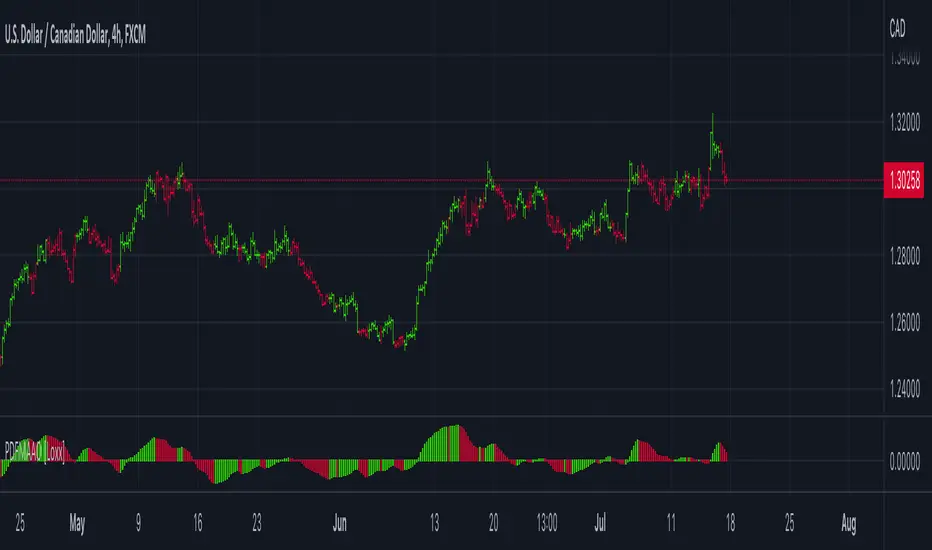
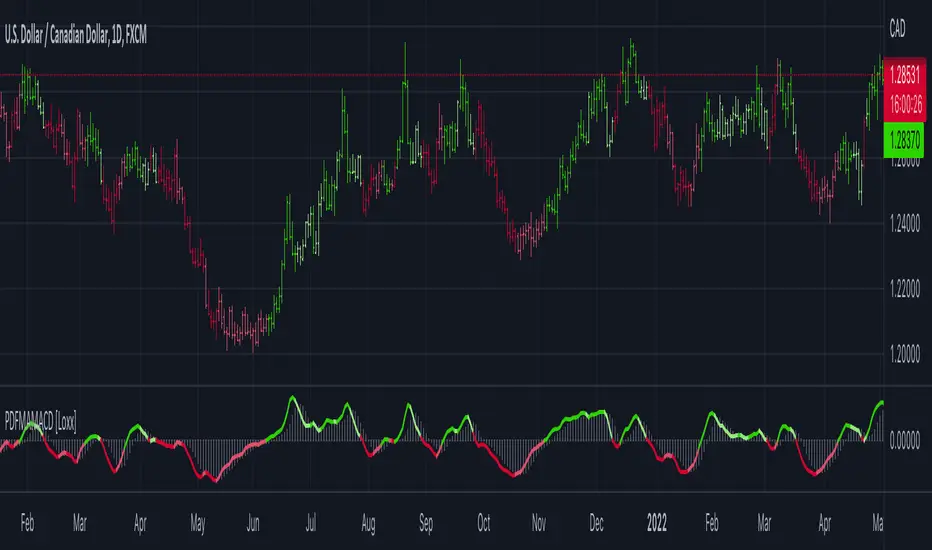
Probability Density Function based MA MACD [Loxx]Probability Density Function based MA MACD is a MACD indicator using a type of weighted moving average.
What is Probability Density Function based MA MACD?
Probability density function based MA is a sort of weighted moving average that uses probability density function to calculate the weights.
Included:
-Toggle on/off bar coloring
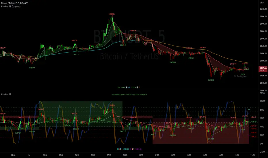
Haydens RSI CompanionPreface: I'm just the bartender serving today's freshly blended concoction; I'd like to send a massive THANK YOU to all the coders and PineWizards for the locally-sourced ingredients. I am simply a code editor, not a code author. The book that inspired this indicator is a free download, plus all of the pieces I used were free code from the community; my hope is that any additional useful development of The Complete RSI is also offered open-source to the community for collaboration.
Features: Fibonacci retracement plus targets. Advanced dual data ticker. Heiken Ashi or bar overlay. Hayden, BarefootJoey, Tradingview, or Custom watermark of choice. Trend lines for spotting wedges, triangles, pennants, etc. Divergences for spotting potential reversals and Momentum Discrepancy Reversal Point opportunities. Percent change and price pivot labels with advanced data & retracement targets upon hover.
‼ IMPORTANT: Hover over labels for advanced information, like targets. Google & read John Hayden's "The Complete RSI" pdf book for comprehensive instructions before attempting to trade with this indicator. Always keep an eye on higher/stronger timeframes. See the companion oscillator here:
⚠ DISCLAIMER: DYOR. Not financial advice. Not a trading system. I am not affiliated with TradingView or John Hayden; this is my own personally PineScripted presentation of a suitable RSI chart companion to use when trading according to Hayden's rules.
About the Editor: I am a former-FINRA Registered Representative, inventor/patent-holder, and self-taught PineScripter. I mostly code on a v3 Pinescript level so expect heavy scripts that could use some shortening with modern conventions.
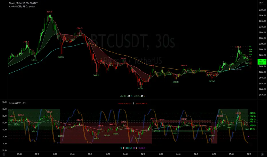
Hayden's Advanced Relative Strength Index (RSI)Preface: I'm just the bartender serving today's freshly blended concoction; I'd like to send a massive THANK YOU to @iFuSiiOnzZ, @Koalafied_3, @LonesomeTheBlue, @LazyBear, @dgtrd and the rest of the PineWizards for the locally-sourced ingredients. I am simply a code editor, not a code author. The book that inspired this indicator is a free download, plus all of the pieces I used were free code from the PineWizards; my hope is that any additional useful development of The Complete RSI trading system also is offered open-source to the community for collaboration.
Features: Fixed & Custom price targeting. Triple trend state detection. Advanced data ticker. Candles, bars, or line RSI . Stochastic of over 20 indicators for adjustable entry/exit signals. Customizable trader watermark. Trend lines for spotting wedges , triangles, pennants , etc. Divergences for spotting potential reversals and Momentum Discrepancy Reversal Point opportunities. RSI percent change and price pivot labels. Gradient bar coloring on-chart.
‼ IMPORTANT: Hover over labels for additional information. Google & read John Hayden's "The Complete RSI" pdf book for comprehensive instructions before attempting to trade with this indicator. Always keep an eye on higher/stronger timeframes.
⚠ DISCLAIMER: DYOR. Not financial advice. Not a trading system. I am not affiliated with TradingView or John Hayden; this is my own personally PineScripted presentation of a suitable RSI to use when trading according to Hayden's rules.
About the Editor: I am a former-FINRA Registered Representative, inventor/patent-holder, and self-taught PineScripter. I mostly code on a v3 Pinescript level so expect heavy scripts that could use some shortening with modern conventions.
Hayden's RSI Rules:
📈 An Uptrend is indicated when:
1. RSI is in the 80 to 40 range
2. The chart shows simple bearish divergence
3. The chart shows Hidden bullish divergence
4. The chart shows Momentum Discrepancy Reversal Up
5. Upside targets being hit
6. 9-bar simple MA is greater than the 45-bar EMA on RSI
7. Counter-trend declines do not exceed 50% of the previous rally
🔮 An Uptrend is in danger when:
1. Longer timeframe fading rally
2. a) Multiple long-term bearish divergences. b) Upside targets not being hit.
3. 9-bar simple MA is less than the 45-bar EMA on RSI
4. Hidden bearish divergence, or simple bullish divergence
5. Deep counter-trend retracements greater than 50%
📉 A Downtrend is indicated when:
1. RSI is in the 60 to 20 range
2. The chart shows simple bullish divergences.
3. The chart shows Hidden bearish divergence
4. The chart shows Momentum Discrepancy Reversal Down
5. Downside targets being hit
6. 9-bar simple MA is less than the 45-bar EMA on RSI
7. Counter-trend rallies do not exceed 50% of the previous decline
🔮 A Downtrend is in danger when:
1. Longer timeframe fading decline
2. a) Multiple long-term bullish divergences. b) Downside targets not being hit.
3. 9-bar simple MA is greater than the 45-bar EMA on RSI
4. Hidden bullish divergence , or simple bearish divergence
5. Steep counter-trend retracements greater than 50%
MathProbabilityDistributionLibrary "MathProbabilityDistribution"
Probability Distribution Functions.
name(idx) Indexed names helper function.
Parameters:
idx : int, position in the range (0, 6).
Returns: string, distribution name.
usage:
.name(1)
Notes:
(0) => 'StdNormal'
(1) => 'Normal'
(2) => 'Skew Normal'
(3) => 'Student T'
(4) => 'Skew Student T'
(5) => 'GED'
(6) => 'Skew GED'
zscore(position, mean, deviation) Z-score helper function for x calculation.
Parameters:
position : float, position.
mean : float, mean.
deviation : float, standard deviation.
Returns: float, z-score.
usage:
.zscore(1.5, 2.0, 1.0)
std_normal(position) Standard Normal Distribution.
Parameters:
position : float, position.
Returns: float, probability density.
usage:
.std_normal(0.6)
normal(position, mean, scale) Normal Distribution.
Parameters:
position : float, position in the distribution.
mean : float, mean of the distribution, default=0.0 for standard distribution.
scale : float, scale of the distribution, default=1.0 for standard distribution.
Returns: float, probability density.
usage:
.normal(0.6)
skew_normal(position, skew, mean, scale) Skew Normal Distribution.
Parameters:
position : float, position in the distribution.
skew : float, skewness of the distribution.
mean : float, mean of the distribution, default=0.0 for standard distribution.
scale : float, scale of the distribution, default=1.0 for standard distribution.
Returns: float, probability density.
usage:
.skew_normal(0.8, -2.0)
ged(position, shape, mean, scale) Generalized Error Distribution.
Parameters:
position : float, position.
shape : float, shape.
mean : float, mean, default=0.0 for standard distribution.
scale : float, scale, default=1.0 for standard distribution.
Returns: float, probability.
usage:
.ged(0.8, -2.0)
skew_ged(position, shape, skew, mean, scale) Skew Generalized Error Distribution.
Parameters:
position : float, position.
shape : float, shape.
skew : float, skew.
mean : float, mean, default=0.0 for standard distribution.
scale : float, scale, default=1.0 for standard distribution.
Returns: float, probability.
usage:
.skew_ged(0.8, 2.0, 1.0)
student_t(position, shape, mean, scale) Student-T Distribution.
Parameters:
position : float, position.
shape : float, shape.
mean : float, mean, default=0.0 for standard distribution.
scale : float, scale, default=1.0 for standard distribution.
Returns: float, probability.
usage:
.student_t(0.8, 2.0, 1.0)
skew_student_t(position, shape, skew, mean, scale) Skew Student-T Distribution.
Parameters:
position : float, position.
shape : float, shape.
skew : float, skew.
mean : float, mean, default=0.0 for standard distribution.
scale : float, scale, default=1.0 for standard distribution.
Returns: float, probability.
usage:
.skew_student_t(0.8, 2.0, 1.0)
select(distribution, position, mean, scale, shape, skew, log) Conditional Distribution.
Parameters:
distribution : string, distribution name.
position : float, position.
mean : float, mean, default=0.0 for standard distribution.
scale : float, scale, default=1.0 for standard distribution.
shape : float, shape.
skew : float, skew.
log : bool, if true apply log() to the result.
Returns: float, probability.
usage:
.select('StdNormal', __CYCLE4F__, log=true)
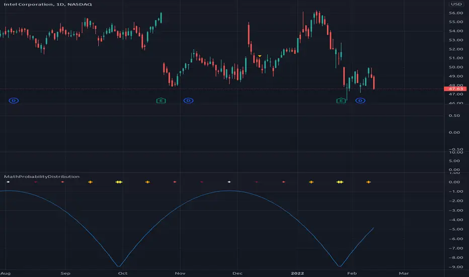
Mobility Oscillator [CC]The Mobility Oscillator was created by Mel Widner (Stocks and Commodities Feb 1996) and this is another of my ongoing series of undiscovered gems. I would say this is probably the most complicated script I have written for an indicator. It is extremely complicated to calculate comparing to other indicators but this is essentially an overbought and oversold indicator that uses a very unique technique to calculate overbought and oversold levels and overall upward or downward momentum there is in the underlying stock. It uses a price distribution function to determine how often the current prices fall within the current trend which tells us how strong the momentum for the current trend actually is. I had to customize this indicator a bit to give clear buy and sell readings so I had to introduce a lag in exchange for clearer signals. This indicator ranges between +100 and -100 and when it stays at the +100 level for example then this means a sustained uptrend and vice versa. I have included strong buy and sell signals in addition to normal ones so strong signals are darker in color and normal signals are lighter in color. Buy when the line turns green and sell when it turns red.
Let me know if there are any other scripts or indicators you would like to see me publish!

Probability Distribution HistogramProbability Distribution Histogram
During data exploration it is often useful to plot the distribution of the data one is exploring. This indicator plots the distribution of data between different bins.
Essentially, what we do is we look at the min and max of the entire data set to determine its range. When we have the range of the data, we decide how many bins we want to divide this range into, so that the more bins we get, the smaller the range (a.k.a. width) for each bin becomes. We then place each data point in its corresponding bin, to see how many of the data points end up in each bin. For instance, if we have a data set where the smallest number is 5 and the biggest number is 105, we get a range of 100. If we then decide on 20 bins, each bin will have a width of 5. So the left-most bin would therefore correspond to values between 5 and 10, and the bin to the right would correspond to values between 10 and 15, and so on.
Once we have distributed all the data points into their corresponding bins, we compare the count in each bin to the total number of data points, to get a percentage of the total for each bin. So if we have 100 data points, and the left-most bin has 2 data points in it, that would equal 2%. This is also known as probability mass (or well, an approximation of it at least, since we're dealing with a bin, and not an exact number).
Usage
This is not an indicator that will give you any trading signals. This indicator is made to help you examine data. It can take any input you give it and plot how that data is distributed.
The indicator can transform the data in a few ways to help you get the most out of your data exploration. For instance, it is usually more accurate to use logarithmic data than raw data, so there is an option to transform the data using the natural logarithmic function. There is also an option to transform the data into %-Change form or by using data differencing.
Another option that the indicator has is the ability to trim data from the data set before plotting the distribution. This can help if you know there are outliers that are made up of corrupted data or data that is not relevant to your research.
I also included the option to plot the normal distribution as well, for comparison. This can be useful when the data is made up of residuals from a prediction model, to see if the residuals seem to be normally distributed or not.

TDI - Traders Dynamic Index + RSI Divergences + Buy/Sell SignalsTraders Dynamic Index + RSI Divergences + Buy/Sell Signals
Credits to LazyBear (original code author) and JustUncleL (modifications)..
I added some new features:
1- RSI Divergences (Original code from 'Divergence Indicator')
2- Buy/Sell Signals with alerts (Green label 'Buy' - Red label 'Sell')
3- Background colouring when RSI (Green line) crosses above MBL (yellow line)
- Buy and Sell Signals are generated using Dean Malone's method (The Author of the TDI indicator) as mentioned in his PDF: (( www.forexfactory.com )), according to:
** Buy (Green Label) = RSI > 50, Red line, & Yellow line
** Sell (Red Label) = RSI < 50, Red line, & Yellow line
- I found that the best quality long trades generated when RSI crosses above red line, yellow line and they are all above 50, and vice versa for sell trades.
-I figured out another way to generate Buy/Sell Signals when RSI crosses above the yellow line, and you can stay with the trade till RSI crosses under the yellow line (I made a background colouring for that to be easily detected)
Hope you all wonderful trades..
مؤلف المؤشر هو (Dean Malone)
وكتب LazyBear كوده في tradingview
وأضاف JustUncleL بعض التعديلات عليه
أضفت إليه بعض المزايا الأخرى المتمثلة في:
1- رصد انحرافات مؤشر القوة النسبية
2- إشارات بيع وشراء بناء على طريقة مؤلف المؤشر
3- تظليل بالأخضر للمنطقة التي يعبر فيها مؤشر القوة النسبية الخط الأوسط (الخط الأصفر)
إشارات البيع والشراء تكون كالتالي:
** الشراء عندما يكون مؤشر القوة النسبية فوق الخط الأحمر وفوق خط الـ 50 وفوق الخط الأصفر
** البيع عندما يكون مؤشر القوة النسبية تحت الخط الأحمر وتحت خط الـ 50 وتحت الخط الأصفر
** أفضل إشارات الشراء حينما يعبر مؤشر القوة النسبية فوق الخط الأحمر والأصفر، ويكونوا جميعا فوق خط الـ 50، والعكس بالنسبة لإشارات البيع
يمكن استخدام المؤشر في دخول صفقات متوسط المدى، وذلك عندما يعبر مؤشر القوة النسبية فوق الخط الأصفر (قمت بتظليل المنطقة بالأخضر لسهولة رصدها) والخروج من الصفقة إذا نزل مؤشر القوة النسبية عن الخط الأصفر،
يرجى التنبه إلى أن الدخول والخروج يكون بأسباب فنية مدروسة، والمؤشر يدعم قراراتك فقط، ولا يمكن الاعتماد عليه منفردا في تحديد نقاط الدخول أوالخروج.
تجارة موفقة لكم جميعا :)
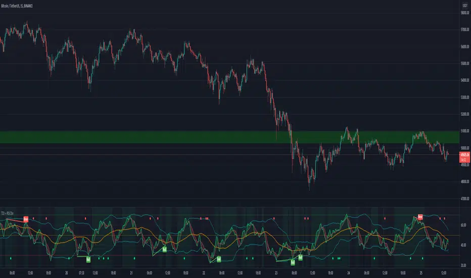
A Useful MA Weighting Function For Controlling Lag & SmoothnessSo far the most widely used moving average with an adjustable weighting function is the Arnaud Legoux moving average (ALMA), who uses a Gaussian function as weighting function. Adjustable weighting functions are useful since they allow us to control characteristics of the moving average such as lag and smoothness.
The following moving average has a simple adjustable weighting function that allows the user to have control over the lag and smoothness of the moving average, we will see that it can also be used to get both an SMA and WMA.
A high-resolution gradient is also used to color the moving average, makes it fun to watch, the plot transition between 200 colors, would be tedious to make but everything was made possible using a custom R script, I only needed to copy and paste the R console output in the Pine editor.
Settings
length : Period of the moving average
-Lag : Setting decreasing the lag of the moving average
+Lag : Setting increasing the lag of the moving average
Estimating Existing Moving Averages
The weighting function of this moving average is derived from the calculation of the beta distribution, advantages of such distribution is that unlike a lot of PDF, the beta distribution is defined within a specific range of values (0,1). Parameters alpha and beta controls the shape of the distribution, with alpha introducing negative skewness and beta introducing positive skewness, while higher values of alpha and beta increase kurtosis.
Here -Lag is directly associated to beta while +Lag is associated with alpha . When alpha = beta = 1 the distribution is uniform, and as such can be used to compute a simple moving average.
Moving average with -Lag = +Lag = 1 , its impulse response is shown below.
It is also possible to get a WMA by increasing -Lag , thus having -Lag = 2 and +Lag = 1 .
Using values of -Lag and +Lag equal to each other allows us to get a symmetrical impulse response, increasing these two values controls the heaviness of the tails of the impulse response.
Here -Lag = +Lag = 3 , note that when the impulse response of a moving average is symmetrical its lag is equal to (length-1)/2 .
As for the gradient, the color is determined by the value of an RSI using the moving average as input.
I don't promise anything but I will try to respond to your comments

[blackcat] L2 Ehlers Fisher Transform of N-bar Price ChannelLevel: 2
Background
John F. Ehlers introuced Fisher Transform of Normalize Price to a N-Day Channel in his "Cybernetic Analysis for Stocks and Futures" chapter 1 on 2004.
Function
The Fisher transform changes the PDF of any waveform so that the transformed output has an approximately Gaussian PDF. So what does this mean for trading? If the prices are normalized to fall within the range from −1 to +1 and subjected to the Fisher transform, extreme price movements are relatively rare events. This means the turning points can be clearly and unambiguously identified.
Key Signal
Fish ---> Fisher transform fast line
Fish ---> Fisher transform slow line
Pros and Cons
100% John F. Ehlers definition translation of original work, even variable names are the same. This help readers who would like to use pine to read his book. If you had read his works, then you will be quite familiar with my code style.
Remarks
The 21th script for Blackcat1402 John F. Ehlers Week publication.
Readme
In real life, I am a prolific inventor. I have successfully applied for more than 60 international and regional patents in the past 12 years. But in the past two years or so, I have tried to transfer my creativity to the development of trading strategies. Tradingview is the ideal platform for me. I am selecting and contributing some of the hundreds of scripts to publish in Tradingview community. Welcome everyone to interact with me to discuss these interesting pine scripts.
The scripts posted are categorized into 5 levels according to my efforts or manhours put into these works.
Level 1 : interesting script snippets or distinctive improvement from classic indicators or strategy. Level 1 scripts can usually appear in more complex indicators as a function module or element.
Level 2 : composite indicator/strategy. By selecting or combining several independent or dependent functions or sub indicators in proper way, the composite script exhibits a resonance phenomenon which can filter out noise or fake trading signal to enhance trading confidence level.
Level 3 : comprehensive indicator/strategy. They are simple trading systems based on my strategies. They are commonly containing several or all of entry signal, close signal, stop loss, take profit, re-entry, risk management, and position sizing techniques. Even some interesting fundamental and mass psychological aspects are incorporated.
Level 4 : script snippets or functions that do not disclose source code. Interesting element that can reveal market laws and work as raw material for indicators and strategies. If you find Level 1~2 scripts are helpful, Level 4 is a private version that took me far more efforts to develop.
Level 5 : indicator/strategy that do not disclose source code. private version of Level 3 script with my accumulated script processing skills or a large number of custom functions. I had a private function library built in past two years. Level 5 scripts use many of them to achieve private trading strategy.
Volatility GuppyBased on my previous script "Turtle N Normalized," this script plots the CM SuperGuppy on the value of N to identify changing trends in the volatility of any instrument.
Turtle rules taken from an online PDF:
"The Turtles used a concept that Richard Dennis and Bill Eckhardt called N to represent the underlying volatility of a particular market.
N is simply the 20-day exponential moving average of the True Range, which is now more commonly known as the ATR. Conceptually, N represents the average range in price movement that a particular market makes in a single day, accounting for opening gaps. N was measured in the same points as the underlying contract.
The Turtles built positions in pieces which we called Units. Units were sized so that 1 N represented 1% of the account equity. Thus, a unit for a given market or commodity can be calculated using the following formula:
Unit = 1% of Account/(N x Dollars per Point)"
To normalize the Unit formula, this script instead takes the value of (close/N). Dollars per point = 1 for stocks and crypto, but will change depending on the contract specifications for individual futures .
"Since the Turtles used the Unit as the base measure for position size, and since those units were volatility risk adjusted, the Unit was a measure of both the risk of a position, and of the entire portfolio of positions."
When the EMA's are green, volatility is decreasing.
When the EMA's are red, volatility is increasing.
When the EMA's are grey, the trend is changing.
