Line Break Chart StrategyHello All!
We should not pass this year without a gift!
My last publication in 2024 is Complete Line Break Chart Strategy with many features!
What is Line Break Chart?
" Line Break is a Japanese chart style that disregards time intervals and only focuses on price movements, similar to the Kagi and Renko chart styles. Line Break charts form a series of up and down bars (referred to as lines). Up lines represent rising prices, and down lines represent falling prices. New confirmed lines only form on the chart when closing prices break the range covered by previous lines. Users can control the number of past lines used in the calculation via the "Number of Lines" input in the chart settings. The typical "Number of Lines" setting is 3, meaning the chart forms a new up line when the closing price is above the high prices of the last three lines, and it forms a new down line when the closing price is below the past three lines' low prices. If the current price is higher, it is an up line and if it is lower, it is a down line. If the current closing price is the same or the move in the opposite direction is not large enough to warrant a reversal, l then no new line is draw n" by Tradingview. You can find it here
Now let's start examining the features of the indicator:
By using Line break reversals it shows trend on the main chart. You can create alert .
Moreover, you can decide which trade should be taken by using Risk Management in the indicator. You can set the " Maximum Risk " and then if the risk is more than you set then the trade is not taken. When trend changed it checks the distance between reversal level and open price and compare it with the Maximum Risk
Breakout:
It can find breakouts and shows on the chart. You can create alert for breakouts
It can show breakouts on the main chart:
Flip-Flops:
Upon looking at set of price break charts, the trader will notice that there are instances when uptrend blocks is followed by one reversal block, and then by a reversal to a series of uptrend blocks. The opposite is also possible: a series of downtrend blocks is followed by one reversal box and then by an immediate reversal to downtrend. This price action is called a " Flip-Flop ". This structure usually produces trend continuation signal. when we see this then we better use Buy/Sell stop order. lets see this on the chart:
Temporal Sequence Table:
Sequence frequency shows the frequency distribution of the number of sequential highs and the number of sequential lows that have been generated. This is quite important to the trader who is seeking to join a trend or put on a trade when the price break reverses into a new trend direction. For example, if the pattern over the past year has been that there never were more than nine consecutive high closes, it would make sense not to enter a position late into the sequence of new high closes.
also you can see market structure. I have tried to formalize it and show it under the table. so you can understand if it's choppy market.
"Number of Lines" has very important role. While using low time frames such seconds/minutes time frame you may want to choose higher number of lines such 5,6. ( this may minimize the risk of a whipsaw )
Gaps feature:
You can set Gaps on/off. if Gaps on then you can see how long it takes for each box
Reversal and Continuation Probability:
The script calculated Reversal level and Continuation probability of the trend by using Sequence frequency.
It also shows unconfirmed box and current closing price level:
Last but not least it has Overlay option for all items, and can show all items in the main chart!
P.S. I added alerts :)
Wish you all a happy new year!
Enjoy!
在腳本中搜尋"雅虎财经+上证指数2024年每天成交额"

Merry Christmas Tree🎄 Merry Christmas 2024 🎅
May your holidays sparkle with joy and laughter, and may the year ahead be full of blessings and success. Wishing you and your loved ones peace, love, and happiness this Christmas and always! 🌟🎁
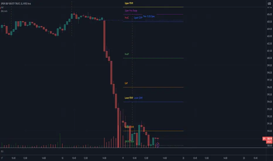
BKLevelsThis displays levels from a text input, levels from certain times on the previous day, and high/low/close from previous day. The levels are drawn for the date in the first line of the text input. Newlines are required between each level
Example text input:
2024-12-17
SPY,606,5,1,Lower Hvol Range,FIRM
SPY,611,1,1,Last 20K CBlock,FIRM
SPY,600,2,1,Last 20K PBlock,FIRM
SPX,6085,1,1,HvolC,FIRM
SPX,6080,2,1,HvolP,FIRM
SPX,6095,3,1,Upper PDVR,FIRM
SPX,6060,3,1,Lower PDVR,FIRM
For each line, the format is ,,,,,
For color, there are 9 possible user- configurable colors- so you can input numbers 1 through 9
For line style, the possible inputs are:
"FIRM" -> solid line
"SHORT_DASH" -> dotted line
"MEDIUM_DASH" -> dashed line
"LONG_DASH" -> dashed line
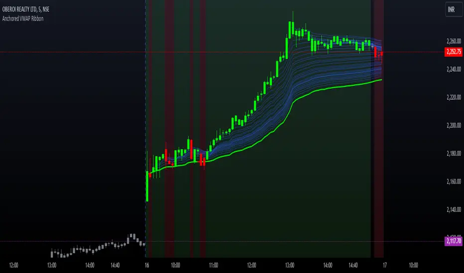
Options Series - Anchored VWAP Ribbon➤ AVWAP On different chart symbols:
⭐ Overview and Key Features:
Anchored VWAP Calculation:
The script implements the Anchored Volume Weighted Average Price (AVWAP), a tool used by professional traders to identify key price levels weighted by volume, starting from a specific timestamp (anchor point).
Bullish and Bearish Analysis:
It determines the dominance of bullish or bearish momentum based on the relationship between the close price and AVWAP levels across multiple time points.
Dynamic Visualization:
The background of the chart changes color based on overall bullish or bearish sentiment, making it easier to interpret market trends.
Multi-Time Anchors:
By defining multiple anchor points (e.g., 09:15, 09:20), the script calculates a series of AVWAP values for fine-grained intraday analysis.
Customizable Inputs:
Users can select the source price (e.g., hlc3), date, and time for AVWAP calculation.
⭐ How It Works and Functionality:
AVWAP Logic:
Uses the timestamp() function to establish a reference (anchor point).
Calculates the cumulative weighted price (price * volume) and cumulative volume from this anchor point.
The ratio of these sums gives the AVWAP, which updates dynamically with new bars.
Bullish and Bearish Signals:
Binary flags (1 or 0) are set for each time point depending on whether the closing price is above or below the AVWAP for that time.
Aggregates these flags into AVWAP_bull and AVWAP_bear to represent the overall market sentiment.
Decision Logic:
Determines final market conditions (bullish or bearish dominance) based on aggregated scores.
Visual feedback (background and bar colors) is applied accordingly.
⭐ Visualizations and User Experience:
Background Colors:
Green or red background highlights the overall sentiment (bullish or bearish), providing a quick market overview.
Bar Coloring:
Bars are color-coded based on bullish, bearish, or neutral conditions, making it easier to identify trends directly on the chart.
AVWAP Levels:
The calculated AVWAP values are plotted as colored lines for each anchor point, giving precise intraday levels of significance.
Bright colors (fluorescent green/red) are used for additional clarity when the close price is above or below these levels.
🎨 Settings and Customization:
Anchor Point:
Fully customizable anchor points allow users to set specific dates and times (e.g., 09:15 on December 13, 2024) for AVWAP calculations.
Source Price:
Users can choose from hlc3, close, or any other price source to calculate the AVWAP, tailoring the indicator to their strategy.
Visual Appearance:
The transparency, colors, and line styles are adjustable, enabling users to customize the chart to match their trading preferences.
Dynamic Signals:
The script accommodates numerous AVWAP levels, providing flexibility for scalpers and swing traders alike.
⭐ Uniqueness of the Concept:
Precise Intraday Analysis:
Unlike static VWAP, this script allows anchoring to specific times during the day, offering granular insights into market behavior.
Cumulative Sentiment Approach:
Aggregates signals across multiple time intervals, providing a comprehensive view of intraday momentum rather than a single-point reference.
Blending AVWAP with Visual Feedback:
Combines traditional AVWAP calculations with visually impactful features like background shading and bar coloring to enhance decision-making.
Scalability:
Supports adding multiple additional anchor points and customization for broader applicability in different market conditions.
🚀 Conclusion:
The Anchored VWAP Ribbon script is a powerful tool for traders seeking to analyze price behavior relative to volume-weighted levels anchored at specific times. It provides a visually intuitive way to assess intraday market sentiment, combining traditional technical indicators with customizable visualization features. The script’s flexibility makes it suitable for a variety of trading styles, from scalping to swing trading, while its unique cumulative sentiment logic sets it apart from conventional VWAP tools.
5x Volume indicator - Day Trading5x Volume Screener - Day Trading
Version: 6.0
Description:
This indicator is designed to identify significant volume spikes in crypto and stock markets,
specifically targeting instances where volume exceeds 5x the average of a 10-period Simple Moving Average (SMA) as the baseline.
Perfect for day traders and momentum traders looking for high-volume breakout opportunities.
Key Features:
Tracks real-time volume compared to 5-period moving average
Visual alerts through green histogram bars for 5x volume spikes
Dynamic volume ratio display showing exact multiple of average volume
Clear threshold line for quick reference
Optional labels showing precise volume ratios
Benefits:
Instantly spot unusual volume activity
Identify potential breakout opportunities
Validate price movements with volume confirmation
Perfect for day trading and scalping
Works across multiple timeframes
Best Used For:
Day trading setups
Breakout trading
Volume confirmation
Momentum trading
Market reversal identification
Created by: CigarSavant
Last Updated: December 2024

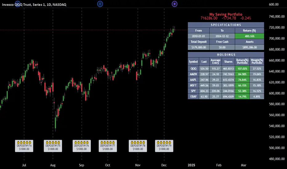
Employee Portfolio Generator [By MUQWISHI]▋ INTRODUCTION :
The “Employee Portfolio Generator” simplifies the process of building a long-term investment portfolio tailored for employees seeking to build wealth through investments rather than traditional bank savings. The tool empowers employees to set up recurring deposits at customizable intervals, enabling to make additional purchases in a list of preferred holdings, with the ability to define the purchasing investment weight for each security. The tool serves as a comprehensive solution for tracking portfolio performance, conducting research, and analyzing specific aspects of portfolio investments. The output includes an index value, a table of holdings, and chart plots, providing a deeper understanding of the portfolio's historical movements.
_______________________
▋ OVERVIEW:
● Scenario (The chart above can be taken as an example) :
Let say, in 2010, a newly employed individual committed to saving $1,000 each month. Rather than relying on a traditional savings account, chose to invest the majority of monthly savings in stable well-established stocks. Allocating 30% of monthly saving to AMEX:SPY and another 30% to NASDAQ:QQQ , recognizing these as reliable options for steady growth. Additionally, there was an admired toward innovative business models of NASDAQ:AAPL , NASDAQ:MSFT , NASDAQ:AMZN , and NASDAQ:EBAY , leading to invest 10% in each of those companies. By the end of 2024, after 15 years, the total monthly deposits amounted to $179,000, which would have been the result of traditional saving alone. However, by sticking into long term invest, the value of the portfolio assets grew, reaching nearly $900,000.
_______________________
▋ OUTPUTS:
The table can be displayed in three formats:
1. Portfolio Index Title: displays the index name at the top, and at the bottom, it shows the index value, along with the chart timeframe, e.g., daily change in points and percentage.
2. Specifications: displays the essential information on portfolio performance, including the investment date range, total deposits, free cash, returns, and assets.
3. Holdings: a list of the holding securities inside a table that contains the ticker, last price, entry price, return percentage of the portfolio's total deposits, and latest weighted percentage of the portfolio. Additionally, a tooltip appears when the user passes the cursor over a ticker's cell, showing brief information about the company, such as the company's name, exchange market, country, sector, and industry.
4. Indication of New Deposit: An indication of a new deposit added to the portfolio for additional purchasing.
5. Chart: The portfolio's historical movements can be visualized in a plot, displayed as a bar chart, candlestick chart, or line chart, depending on the preferred format, as shown below.
_______________________
▋ INDICATOR SETTINGS:
Section(1): Table Settings
(1) Naming the index.
(2) Table location on the chart and cell size.
(3) Sorting Holdings Table. By securities’ {Return(%) Portfolio, Weight(%) Portfolio, or Ticker Alphabetical} order.
(4) Choose the type of index: {Assets, Return, or Return (%)}, and the plot type for the portfolio index: {Candle, Bar, or Line}.
(5) Positive/Negative colors.
(6) Table Colors (Title, Cell, and Text).
(7) To show/hide any of selected indicator’s components.
Section(2): Recurring Deposit Settings
(1) From DateTime of starting the investment.
(2) To DateTime of ending the investment
(3) The amount of recurring deposit into portfolio and currency.
(4) The frequency of recurring deposits into the portfolio {Weekly, 2-Weeks, Monthly, Quarterly, Yearly}
(5) The Depositing Model:
● Fixed: The amount for recurring deposits remains constant throughout the entire investment period.
● Increased %: The recurring deposit amount increases at the selected frequency and percentage throughout the entire investment period.
(5B) If the user selects “ Depositing Model: Increased % ”, specify the growth model (linear or exponential) and define the rate of increase.
Section(3): Portfolio Holdings
(1) Enable a ticker in the investment portfolio.
(2) The selected deposit frequency weight for a ticker. For example, if the monthly deposit is $1,000 and the selected weight for XYZ stock is 30%, $300 will be used to purchase shares of XYZ stock.
(3) Select up to 6 tickers that the investor is interested in for long-term investment.
Please let me know if you have any questions
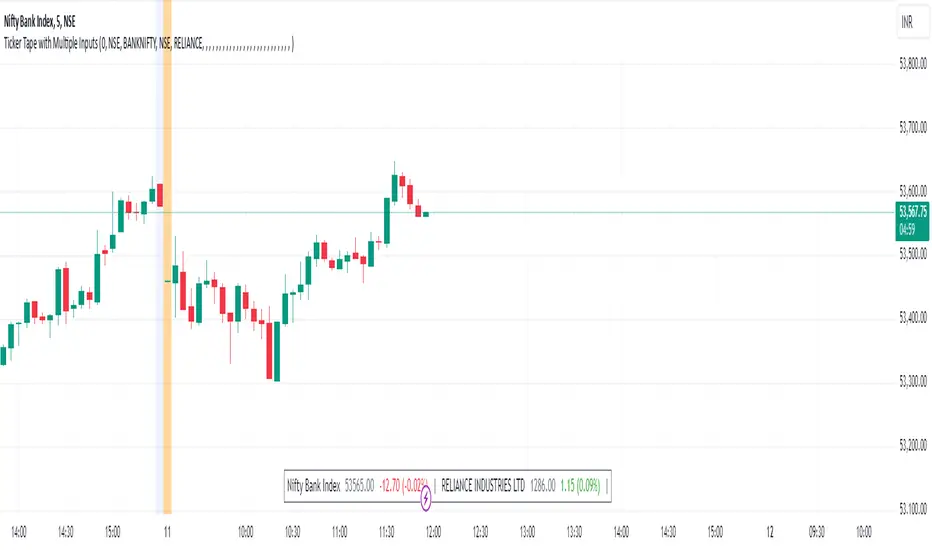
Ticker Tape with Multiple Inputs# Ticker Tape
A customizable multi-symbol price tracker that displays real-time price information in a scrolling ticker format, similar to financial news tickers.
This indicator is inspired from Tradingciew's default tickertape indicator with changes in the way inputs are given.
### Overview
This indicator allows you to monitor up to 15 different symbols simultaneously across any supported exchanges on TradingView. It displays essential price information including current price, price change, and percentage change in an easy-to-read format at the bottom of your chart.
### Features
• Monitor up to 15 different symbols simultaneously
• Support for any exchange available on TradingView
• Real-time price updates
• Color-coded price changes (green for increase, red for decrease)
• Smooth scrolling animation (can be disabled)
• Customizable scroll speed and position offset
### Input Parameters
#### Ticker Tape Controls
• Running: Enable/disable the scrolling animation
• Offset: Adjust the starting position of the ticker tape
#### Symbol Settings
• Exchange (1-15): Enter the exchange name (e.g., NSE, BINANCE, NYSE)
• Symbol (1-15): Enter the symbol name (e.g., BANKNIFTY, RELIANCE, BTCUSDT)
### Display Format
For each symbol, the ticker shows:
1. Symbol Name
2. Current Price
3. Price Change (Absolute and Percentage)
### Example Usage
Input Settings:
Exchange 1: NSE
Symbol 1: BANKNIFTY
Exchange 2: NSE
Symbol 2: RELIANCE
The ticker tape will display:
`NIFTY BANK 46750.00 +350.45 (0.75%) | RELIANCE 2456.85 -12.40 (-0.50%) |`
### Use Cases
1. Multi-Market Monitoring: Track different markets simultaneously without switching between charts
2. Portfolio Tracking: Monitor all your positions in real-time
### Tips for Best Use
1. Group related symbols together for easier monitoring
2. Use the offset parameter to position important symbols in your preferred viewing area
3. Disable scrolling if you prefer a static display
4. Leave exchange field empty for default exchange symbols
### Notes
• Price updates occur in real-time during market hours
• Color coding helps quickly identify price direction
• The indicator adapts to any chart timeframe
• Empty input pairs are automatically skipped
### Performance Considerations
The indicator is optimized for efficiency, but monitoring too many high-frequency symbols might impact chart performance. It's recommended to use only the symbols you actively need to monitor.
Version: 2.0 Stock_Cloud
Last Updated: December 2024
Kalman Filter Oscillator v4The Kalman Filter Oscillator v4 is an advanced tool designed to help traders and investors identify trends more effectively while reducing the impact of market noise. As the latest iteration in its development, this version integrates improvements that make it more adaptive and precise, catering to the challenges of today’s financial markets.
This indicator operates on the principle of the Kalman filter, a well-regarded mathematical approach used for estimating the state of a dynamic system. By filtering out random fluctuations, it smooths price data to provide clearer insights into underlying trends. Unlike traditional methods such as moving averages, which often lag and can miss rapid shifts, the Kalman Filter Oscillator is reactive in real time, making it particularly suited for dynamic markets.
Version v4 builds on earlier versions by offering a refined combination of short-term and long-term trend analysis. Through adjustable parameters, traders can balance sensitivity to immediate price changes with a broader perspective of the market direction. Additionally, the oscillator incorporates a unique feature that tracks a price’s position relative to its recent highs and lows, which enhances its ability to pinpoint potential turning points or key market conditions.
The indicator’s value lies in its adaptability and practicality. Traders can use it to confirm trends, identify overbought or oversold conditions, or smooth out erratic price movements, reducing the likelihood of false signals. By presenting information in a clear and actionable format, it allows users to make better-informed decisions with greater confidence.
As of late 2024, the Kalman Filter Oscillator v4 represents a sophisticated yet user-friendly advancement in trend analysis. While not a one-size-fits-all solution, it serves as a valuable component in a trader’s toolkit, complementing other strategies and enhancing overall market understanding.

Alans Date Range CalculatorOverview
Setting a date range for backtesting enables you to evaluate your trading strategy under various market conditions. Traders can test a strategy’s performance during specific periods, such as economic downturns, bull markets, or periods of high volatility. This helps assess the trading strategy’s robustness and adaptability across different scenarios.
Specifying years of data instead of just inputting specific start and end dates offers several advantages:
1. **Consistency**: Using a fixed number of years ensures that the testing period is consistent across different strategies or iterations. This makes it easier to compare performance metrics and draw meaningful conclusions.
2. **Flexibility**: Specifying years allows for automatic adjustment of the start date based on the current date or selected end date. This is particularly useful when new data becomes available or when testing on different assets with varying historical data lengths.
3. **Efficiency**: It simplifies updating and retesting strategies. Instead of recalculating specific start dates each time, traders can quickly adjust the number of years to process, making it easier to test strategies over different timeframes.
4. **Comprehensive Analysis**: Broader timeframes defined by years help you evaluate how your strategy performs over multiple market cycles, providing insights into long-term viability and potential weaknesses.
Defining a date range by specifying years allows for more thorough and systematic backtesting, helping traders develop more reliable and effective trading systems.
Alan's Date Range Calculator: A TradingView Pine Script Indicator
Purpose
This Pine Script indicator calculates and displays a date range for backtesting trading strategies. It allows users to specify the number of years to analyze and an end date, then calculates the corresponding start date. Most importantly, users can copy the inputs and function into their own strategies to quickly add a time span feature for backtesting.
Key Features
User-defined input for the number of years to analyze
Customizable end date with a calendar input
Automatic calculation of the start date
Visual display of both start and end dates on the chart
How It Works
User Inputs
Years of Data to Process: An integer input allowing users to specify the number of years for analysis (default: 20, range: 1-100)
End Date: A calendar input for selecting the end date of the analysis period (default: December 31, 2024)
Date Calculation
The script uses a custom function calcStartDate() to determine the start date. It subtracts the specified number of years from the end date's year and sets the start date to January 1st of that year.
Visual Output
The indicator displays two labels on the chart:
Start Date Label: Shows the calculated start date
End Date Label: Displays the user-specified end date
Both labels are positioned horizontally at the bottom of the chart, with the end date label to the right of the start date label.
Applications
This indicator is particularly useful for traders who want to:
Define specific date ranges for backtesting strategies
Quickly visualize the time span of their analysis
Ensure consistent testing periods across different strategies or assets
Customization
Users can easily adjust the analysis period by changing the number of years or selecting a different end date. This flexibility allows for testing strategies across various market conditions and time frames.

MACD, ADX & RSI -> for altcoins# MACD + ADX + RSI Combined Indicator
## Overview
This advanced technical analysis tool combines three powerful indicators (MACD, ADX, and RSI) into a single view, providing a comprehensive analysis of trend, momentum, and divergence signals. The indicator is designed to help traders identify potential trading opportunities by analyzing multiple aspects of price action simultaneously.
## Components
### 1. MACD (Moving Average Convergence Divergence)
- **Purpose**: Identifies trend direction and momentum
- **Components**:
- Fast EMA (default: 12 periods)
- Slow EMA (default: 26 periods)
- Signal Line (default: 9 periods)
- Histogram showing the difference between MACD and Signal line
- **Visual**:
- Blue line: MACD line
- Orange line: Signal line
- Green/Red histogram: MACD histogram
- **Interpretation**:
- Histogram color changes indicate potential trend shifts
- Crossovers between MACD and Signal lines suggest entry/exit points
### 2. ADX (Average Directional Index)
- **Purpose**: Measures trend strength and direction
- **Components**:
- ADX line (default threshold: 20)
- DI+ (Positive Directional Indicator)
- DI- (Negative Directional Indicator)
- **Visual**:
- Navy blue line: ADX
- Green line: DI+
- Red line: DI-
- **Interpretation**:
- ADX > 20 indicates a strong trend
- DI+ crossing above DI- suggests bullish momentum
- DI- crossing above DI+ suggests bearish momentum
### 3. RSI (Relative Strength Index)
- **Purpose**: Identifies overbought/oversold conditions and divergences
- **Components**:
- RSI line (default: 14 periods)
- Divergence detection
- **Visual**:
- Purple line: RSI
- Horizontal lines at 70 (overbought) and 30 (oversold)
- Divergence labels ("Bull" and "Bear")
- **Interpretation**:
- RSI > 70: Potentially overbought
- RSI < 30: Potentially oversold
- Bullish/Bearish divergences indicate potential trend reversals
## Alert System
The indicator includes several automated alerts:
1. **MACD Alerts**:
- Rising to falling histogram transitions
- Falling to rising histogram transitions
2. **RSI Divergence Alerts**:
- Bullish divergence formations
- Bearish divergence formations
3. **ADX Trend Alerts**:
- Strong trend development (ADX crossing threshold)
- DI+ crossing above DI- (bullish)
- DI- crossing above DI+ (bearish)
## Settings Customization
All components can be fine-tuned through the settings panel:
### MACD Settings
- Fast Length
- Slow Length
- Signal Smoothing
- Source
- MA Type options (SMA/EMA)
### ADX Settings
- Length
- Threshold level
### RSI Settings
- RSI Length
- Source
- Divergence calculation toggle
## Usage Guidelines
### Entry Signals
Strong entry signals typically occur when multiple components align:
1. MACD histogram color change
2. ADX showing strong trend (>20)
3. RSI showing divergence or leaving oversold/overbought zones
### Exit Signals
Consider exits when:
1. MACD crosses signal line in opposite direction
2. ADX shows weakening trend
3. RSI reaches extreme levels with divergence
### Risk Management
- Use the indicator as part of a complete trading strategy
- Combine with price action and support/resistance levels
- Consider multiple timeframe analysis for confirmation
- Don't rely solely on any single component
## Technical Notes
- Built for TradingView using Pine Script v5
- Compatible with all timeframes
- Optimized for real-time calculation
- Includes proper error handling and NA value management
- Memory-efficient calculations for smooth performance
## Installation
1. Copy the provided Pine Script code
2. Open TradingView Chart
3. Create New Indicator -> Pine Editor
4. Paste the code and click "Add to Chart"
5. Adjust settings as needed through the indicator settings panel
## Version Information
- Version: 2.0
- Last Updated: November 2024
- Platform: TradingView
- Language: Pine Script v5

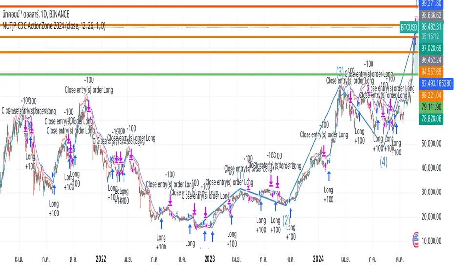
NUTJP CDC ActionZone 20241. Core Components of the Strategy
• Fast EMA and Slow EMA:
• The Fast EMA (shorter period) is more reactive to recent price changes.
• The Slow EMA (longer period) reacts slower and provides a smoother view of the overall trend.
• Relationship Between Fast EMA and Slow EMA:
• When the Fast EMA is above the Slow EMA, the market is considered Bullish.
• When the Fast EMA is below the Slow EMA, the market is considered Bearish.
2. Zones Based on Price and EMAs
The strategy defines six zones based on the position of the price, Fast EMA, and Slow EMA:
1. Green Zone (Buy):
• Bullish trend (Fast EMA > Slow EMA)
• Price is above the Fast EMA.
• Indicates a strong uptrend and suggests buying.
2. Blue and Light Blue Zones (Pre-Buy):
• Price is above the Fast EMA but below or near the Slow EMA.
• Represents potential bullish signals but not strong enough to trigger a buy.
3. Red Zone (Sell):
• Bearish trend (Fast EMA < Slow EMA)
• Price is below the Fast EMA.
• Indicates a strong downtrend and suggests selling or avoiding long trades.
4. Orange and Yellow Zones (Pre-Sell):
• Price is below the Fast EMA but above or near the Slow EMA.
• Represents potential bearish signals but not strong enough to trigger a sell.
These zones help traders visualize the market conditions and determine whether to buy, hold, or sell.
3. Buy and Sell Conditions
• Buy Condition:
A buy signal is triggered when:
• The price enters the Green Zone (Bullish trend and price > Fast EMA).
• It’s the first green candle after a non-green candle.
• Sell Condition:
A sell signal is triggered when:
• The price enters the Red Zone (Bearish trend and price < Fast EMA).
• It’s the first red candle after a non-red candle.
4. Trade Execution Logic
• Buy:
The strategy enters a long position (buy) when the above buy condition is met.
• Sell:
The strategy exits the long position when the sell condition is met.
Note: It doesn’t support short trades, meaning it doesn’t enter sell positions.
5. Momentum-Based Signals (Optional)
The indicator also includes momentum signals using Stochastic RSI to provide additional buy/sell signals:
• These are based on oversold and overbought levels of the Stochastic RSI.
• It filters signals depending on whether the trend is Bullish or Bearish.
6. Visual Features
The indicator is designed to make the trading zones and signals visually intuitive:
• Bar Colors:
Candlesticks are colored based on the current zone (e.g., Green for Buy, Red for Sell).
• EMA Lines:
The Fast EMA and Slow EMA are plotted, making it easy to see crossover points.
• Buy/Sell Signals:
Marked with shapes (e.g., circles) below/above bars for clarity.
7. Strategy Assumptions
• Trend-Following Nature:
This strategy assumes that trends persist. It works best in trending markets but might give false signals in ranging markets.
• Lagging Nature of EMAs:
As EMAs are lagging indicators, buy and sell signals may occur after significant moves have already begun or ended.
• Momentum Confirmation (Optional):
Adding momentum signals can help filter false signals, though it’s not part of the core logic.
8. Usage Recommendations
• Timeframes:
Works on various timeframes but may perform better on higher timeframes (e.g., 1H, Daily) to reduce noise.
• Markets:
Can be applied to stocks, forex, and cryptocurrencies.
• Backtesting and Optimization:
Before live trading, backtest the strategy with different EMA periods and other parameters to find optimal settings for your market and timeframe.
Multi-Symbol Scanner: Advanced EMA-RSI-Volume Strategy# Multi-Symbol Tech Stock Scanner: Advanced EMA-RSI-Volume Strategy
## Technical Analysis Methodology
This scanner implements a sophisticated multi-timeframe analysis approach combining three key technical elements:
### 1. Dual EMA System (Primary Trend Detection)
- **Long-term EMA (820 periods)**: Acts as the primary trend identifier
- Chosen specifically for tech stocks' longer-term price waves
- Helps filter out minor market noise while capturing major trend changes
- 820 periods approximately represents 3.2 years of trading days
- **Medium-term EMA (320 periods)**: Serves as trend confirmation
- Approximately 1.25 years of trading data
- Provides earlier entry signals while maintaining trend reliability
- Helps identify potential trend reversals before the major trend shift
### 2. Volume Analysis Component
The script employs a dynamic volume analysis system:
- Calculates 20-period moving average of volume as baseline
- Requires 1.5x surge above baseline for signal confirmation
- Volume surge requirement helps filter out weak moves and potential false breakouts
- Different from standard volume indicators as it uses adaptive thresholds
### 3. RSI Momentum Filter
Implements a specialized RSI configuration:
- 14-period RSI with dynamic overbought/oversold levels
- Oversold threshold: 30 (customizable)
- Overbought threshold: 70 (customizable)
- Used as a confirmation tool rather than primary signal generator
## Signal Generation Logic
### Buy Signal Requirements
1. Price must cross above 820 EMA (PRIMARY CONDITION)
2. Current price must be above 320 EMA (CONFIRMATION)
3. RSI must be above 30 but below 70 (MOMENTUM CHECK)
4. Volume must be 1.5x above 20-period average (STRENGTH VALIDATION)
### Sell Signal Requirements
1. Price must cross below 820 EMA (PRIMARY CONDITION)
2. Current price must be below 320 EMA (CONFIRMATION)
3. RSI must be above 30 but below 70 (MOMENTUM CHECK)
4. Volume must be 1.5x above 20-period average (STRENGTH VALIDATION)
## Risk Management Integration
The script automatically calculates key risk levels based on volatility:
1. **Stop Loss Calculation**:
- Default: 2% below entry for buys
- Dynamically adjusted based on price point
- Can be modified through input parameters
2. **Take Profit Targets**:
- Primary target: 6% above entry (3:1 reward-risk ratio)
- Based on historical tech stock movement patterns
- Adjustable through input parameters
## Multi-Symbol Implementation
The scanner monitors 6 symbols simultaneously using:
- Separate security calls for each data point
- Optimized data requests to prevent overload
- Individual signal processing for each symbol
- Synchronized alert generation system
## Technical Implementation Details
1. **Data Processing**:
```
- Security data requests on 10-minute timeframe
- Individual EMA calculations per symbol
- Separate volume analysis threads
- RSI calculations with standard deviation normalization
```
2. **Signal Processing**:
```
- Cross-verification of all conditions
- Time-based signal validation
- Volume surge confirmation
- Trend alignment check
```
3. **Alert System**:
```
- Bar-close confirmation required
- Multi-condition validation
- Detailed price level inclusion
- Risk parameter integration
```
## Optimization Features
1. **Memory Usage**:
- Optimized security calls
- Efficient data structure
- Reduced redundant calculations
2. **Processing Efficiency**:
- Single-pass data analysis
- Combined indicator calculations
- Streamlined alert generation
## Practical Application
The system is designed for:
1. Swing Trading (primary use)
2. Position Trading (secondary use)
3. Technical Breakout Trading
Optimal timeframes:
- Primary: 4H charts
- Secondary: Daily charts
- Verification: 1H charts
## Default Configuration
The scanner is preset to monitor key tech stocks:
- TSLA: High-volatility tech leader
- NVDA: Semiconductor sector benchmark
- AVGO: Stable tech infrastructure
- TSM: Global chip manufacturer
- META: Social media sector leader
- AMZN: E-commerce/Cloud computing leader
Each symbol can be modified through input parameters.
## Version Information
- Current Version: 1.3
- Last Updated: November 2024
- Compatibility: TradingView Pro/Pro+/Premium
## Limitations & Considerations
- Limited to 6 symbols due to TradingView security request limits
- Requires consistent market volume for optimal performance
- Best suited for liquid stocks with significant daily volume
- May need parameter adjustments during extreme market conditions

MERCURY by DrAbhiramSivprasad"MERCURY by DrAbhiramSivprasad"
Developed from over 10 years of personal trading experience, the Mercury Indicator is a strategic tool designed to enhance accuracy in trading decisions. Think of it as a guiding light—a supportive tool that helps traders refine and build more robust strategies by integrating multiple powerful elements into a single indicator. I’ll be sharing some examples to illustrate how I use this indicator in my own trading journey, highlighting its potential to improve strategy accuracy.
Reason behind the combination of emas , cpr and vwap is it provides very good support and resistance in my trading carrier so now i brought them together in one plate
How It Works:
Mercury combines three essential elements—EMA, VWAP, and CPR—each of which plays a vital role in detecting support and resistance:
Exponential Moving Averages (EMAs): Known for their strength in providing dynamic support and resistance levels, EMAs help in identifying trends and shifts in momentum. This indicator includes a dashboard with up to nine customizable EMAs, showing whether each is acting as support or resistance based on real-time price movement.
Volume Weighted Average Price (VWAP): VWAP also provides valuable support and resistance, often regarded as a fair price level by institutional traders. Paired with EMAs, it forms a dual-layered support/resistance system, adding an additional level of confirmation.
Central Pivot Range (CPR): By combining CPR with EMAs and VWAP, Mercury highlights “traffic blocks” in your target journey. This means it identifies zones where price is likely to stall or reverse, providing additional guidance for navigating entries and exits.
Why This Combination Matters:
Using these three tools together gives you a more complete view of the market. VWAP and EMAs offer dynamic trend direction and support/resistance, while CPR pinpoints critical price zones. This combination helps you find high-probability trades, adding clarity to complex market situations and enabling stronger confirmation on trend or reversal decisions.
How to Use:
Trend Confirmation: Check if all EMAs are aligned (green for uptrend, red for downtrend), which is visible in the EMA dashboard. An alignment across VWAP, CPR, and EMAs signifies high confidence in trend direction.
Breakouts & Breakdowns: Mercury has an alert system to signal when a price breakout or breakdown occurs across VWAP, EMA1, and EMA2. This can help in spotting strong directional moves.
Example Application: In my trading, I use Mercury to identify support/resistance zones, confirming trends with EMA/VWAP alignment and using CPR as a checkpoint. I find this especially useful for day trading and swing setups.
Recommended Timeframes:
Day Trading: 5 to 15-minute charts for swift, actionable insights.
Swing Trading: 1-hour or 4-hour charts for broader trend analysis.
Note:
The Mercury Indicator should be used as a supportive tool rather than a standalone strategy, guiding you toward informed decisions in line with your trading style and goals.
EXAMPLE OF TRADE
you can see the cart of XAUUSD on 11th nov 2024
1.SHORT POSITION - TIME FRAME 15 MIN
So here for a short position you need to wait for a breakdown candle which will print in orange post the candle you need to check ema dashboard is completly red that indicates no traffic blocks in your journey to destiny target from ema's and you can take the target from nearest cpr support line
TAKEN IN XAUUSD you can see in chart of XAUUSD on 7th nov
2.LONG POSITION - TIME FRAME 15 MIN -
So here for long position you need to wait for a breakout candle from indicator thats here is blue and check all ema boxes are green and candle body should close above all the 3 lines here it is the both ema 1 and 2 and the vwap line then you can take and entry and your target will be the nearest resistance from the daily cpr
3. STOP LOSS CRITERIA
After the entry any candle close below any of the last line from entry for example we have 3 lines vwap and ema 1 and 2 lines and u have made an entry and the last line before the entry is vwap then if any candle closes below vwap can be considered as stoploss like wise in any lines
The MERCURY indicator is a comprehensive trading tool designed to enhance traders' ability to identify trends, breakouts, and reversals effectively. Created by Dr. Abhiram Sivprasad, this indicator integrates several technical elements, including Central Pivot Range (CPR), EMA crossovers, VWAP levels, and a table-based EMA dashboard, to offer a holistic trading view.
Core Components and Functionality:
Central Pivot Range (CPR):
The CPR in MERCURY provides a central pivot level along with Below Central (BC) and Top Central (TC) pivots. These levels act as potential support and resistance, useful for identifying reversal points and zones where price may consolidate.
Exponential Moving Averages (EMAs):
MERCURY includes up to nine EMAs, with a customizable EMA crossover alert system. This feature enables traders to see shifts in trend direction, especially when shorter EMAs cross longer ones.
VWAP (Volume-Weighted Average Price):
VWAP is incorporated as a dynamic support/resistance level and, combined with EMA crossovers, helps refine entry and exit points for higher probability trades.
Breakout and Breakdown Alerts:
MERCURY monitors conditions for upside and downside breakouts. For an upside breakout, all EMAs turn green and a candle closes above VWAP, EMA1, and EMA2. Similarly, all EMAs turning red, combined with a close below VWAP and EMA1/EMA2, signals a downside breakdown. Continuous alerts are available until the trend shifts.
Real-Time EMA Dashboard:
A table displays each EMA’s relative position (Above or Below), helping traders quickly gauge trend direction. Colors in the table adjust to long/short conditions based on EMA alignment.
Usage Recommendations:
Trend Confirmation:
Use the CPR, EMA alignments, and VWAP to confirm uptrends and downtrends. The table highlights trends, making it easy to spot long or short setups at a glance.
Breakout and Breakdown Alerts:
The alert system is customizable for continuous notifications on critical price levels. When all EMAs align in one direction (green for long, red for short) and the close is above or below VWAP and key EMAs, the indicator confirms a breakout/breakdown.
Adaptable for Different Styles:
Day Trading: Traders can set shorter EMAs for quick insights.
Swing Trading: Longer EMAs combined with CPR offer insights into sustained trends.
Recommended Settings:
Timeframes: MERCURY is suitable for timeframes as low as 5 minutes for intraday traders, up to daily charts for trend analysis.
Symbols: Works across forex, stocks, and crypto. Adjust EMA lengths for asset volatility.
Example Strategy:
Long Entry: When the price crosses above CPR and closes above both EMA1 and EMA2.
Short Entry: When the price falls below CPR with a close below both EMA1 and EMA2.

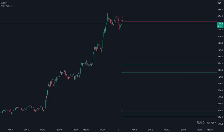
Dynamic Open Levels# Dynamic Open Levels Indicator v1.0
Release Date: November 5, 2024
Introducing the Dynamic Open Levels indicator on TradingView! This tool helps traders visualize and analyze key opening price levels across multiple timeframes, making your market analysis more effective.
---
### Key Features
- Multiple Timeframes : Yearly, Quarterly, Monthly, Weekly, Daily, 4H, and 1H levels available.
- Visibility Controls : Easily toggle visibility for each timeframe to suit your trading style.
- Line Customization : Set custom thickness and colors for lines, making charts easy to interpret.
- Monthly: Purple
- Weekly: Blue
- Daily: Green
- 4H: Red
- 1H: Orange
- Dynamic Coloring : Lines adjust color based on market conditions—teal for bullish (`rgb(34, 171, 148)`) and coral for bearish (`rgb(247, 82, 95)`).
### Labels & Customization
- Real-Time Labels : Each level is labeled for easy identification (e.g., Y for Yearly, Q for Quarterly).
- Label Settings : Customize opacity, text color, size, and position for clarity without cluttering your chart.
- Sizes : Choose from tiny, small, normal, large, to huge.
- Offset : Set labels from 1 to 10 to position them precisely.
- Color Management : Organize all colors under a dedicated Line Colors group for easy adjustments.
### Advanced Plotting & Performance
- Real-Time Updates : Levels are updated dynamically with the latest open prices.
- Extended Lines : Lines extend to the right, offering a consistent reference for future price movement.
- Optimized Performance : Handles up to 500 lines efficiently to maintain smooth performance.
---
### Installation Instructions
1. Add to Chart :
- Go to the Indicators section in TradingView.
- Search for Dynamic Open Levels and add it to your chart.
2. Customize Settings :
- Line Thickness : Adjust to suit your preference.
- Visibility : Toggle timeframes like Yearly, Monthly, Weekly, etc., as needed.
- Labels : Configure opacity, text color, size, and offset under the Label Settings group.
---
### Documentation & Support
For guidance on using the Dynamic Open Levels indicator, visit our Documentation (#). If you need assistance, check out our Support Channel (#).
---
Thank you for choosing Dynamic Open Levels . Stay tuned for future updates that will continue to improve your trading experience!
H A Z E D
Pulse DPO: Major Cycle Tops and Bottoms█ OVERVIEW
Pulse DPO is an oscillator designed to highlight Major Cycle Tops and Bottoms .
It works on any market driven by cycles. It operates by removing the short-term noise from the price action and focuses on the market's cyclical nature.
This indicator uses a Normalized version of the Detrended Price Oscillator (DPO) on a 0-100 scale, making it easier to identify major tops and bottoms.
Credit: The DPO was first developed by William Blau in 1991.
█ HOW TO READ IT
Pulse DPO oscillates in the range between 0 and 100. A value in the upper section signals an OverBought (OB) condition, while a value in the lower section signals an OverSold (OS) condition.
Generally, the triggering of OB and OS conditions don't necessarily translate into swing tops and bottoms, but rather suggest caution on approaching a market that might be overextended.
Nevertheless, this indicator has been customized to trigger the signal only during remarkable top and bottom events.
I suggest using it on the Daily Time Frame , but you're free to experiment with this indicator on other time frames.
The indicator has Built-in Alerts to signal the crossing of the Thresholds. Please don't act on an isolated signal, but rather integrate it to work in conjunction with the indicators present in your Trading Plan.
█ OB SIGNAL ON: ENTERING OVERBOUGHT CONDITION
When Pulse DPO crosses Above the Top Threshold it Triggers ON the OB signal. At this point the oscillator line shifts to OB color.
When Pulse DPO enters the OB Zone, please beware! In this Area the Major Players usually become Active Sellers to the Public. While the OB signal is On, it might be wise to Consider Selling a portion or the whole Long Position.
Please note that even though this indicator aims to focus on major tops and bottoms, a strong trending market might trigger the OB signal and stay with it for a long time. That's especially true on young markets and on bubble-mode markets.
█ OB SIGNAL OFF: EXITING OVERBOUGHT CONDITION
When Pulse DPO crosses Below the Top Threshold it Triggers OFF the OB signal. At this point the oscillator line shifts to its normal color.
When Pulse DPO exits the OB Zone, please beware because a Major Top might just have occurred. In this Area the Major Players usually become Aggressive Sellers. They might wind up any remaining Long Positions and Open new Short Positions.
This might be a good area to Open Shorts or to Close/Reverse any remaining Long Position. Whatever you choose to do, it's usually best to act quickly because the market is prone to enter into panic mode.
█ OS SIGNAL ON: ENTERING OVERSOLD CONDITION
When Pulse DPO crosses Below the Bottom Threshold it Triggers ON the OS signal. At this point the oscillator line shifts to OS color.
When Pulse DPO enters the OS Zone, please beware because in this Area the Major Players usually become Active Buyers accumulating Long Positions from the desperate Public.
While the OS signal is On, it might be wise to Consider becoming a Buyer or to implement a Dollar-Cost Averaging (DCA) Strategy to build a Long Position towards the next Cycle. In contrast to the tops, the OS state usually takes longer to resolve a major bottom.
█ OS SIGNAL OFF: EXITING OVERSOLD CONDITION
When Pulse DPO crosses Above the Bottom Threshold it Triggers OFF the OS signal. At this point the oscillator line shifts to its normal color.
When Pulse DPO exits the OS Zone, please beware because a Major Bottom might already be in place. In this Area the Major Players become Aggresive Buyers. They might wind up any remaining Short Positions and Open new Long Positions.
This might be a good area to Open Longs or to Close/Reverse any remaining Short Positions.
█ WHY WOULD YOU BE INTERESTED IN THIS INDICATOR?
This indicator is built over a solid foundation capable of signaling Major Cycle Tops and Bottoms across many markets. Let's see some examples:
Early Bitcoin Years: From 0 to 1242
This chart is in logarithmic mode in order to properly display various exponential cycles. Pulse DPO is properly signaling the major early highs from 9-Jun-2011 at 31.50, to the next one on 9-Apr-2013 at 240 and the epic top from 29-Nov-2013 at 1242.
Due to the massive price movements, the OB condition stays pinned during most of the exponential price action. But as you can see, the OB condition quickly vanishes once the Cycle Top has been reached. As the market matures, the OB condition becomes more exceptional and triggers much closer from the Cycle Top.
With regards to Cycle Bottoms, the early bottom of 2 after having peaked at 31.50 doesn’t get captured by the indicator. That is the only cycle bottom that escapes the Pulse DPO when the bottom threshold is set at a value of 5. In that event, the oscillator low reached 6.95.
Bitcoin Adoption Spreading: From 257 to 73k
This chart is in logarithmic mode in order to properly display various exponential cycles. Pulse DPO is properly signaling all the major highs from 17-Dec-2017 at 19k, to the next one on 14-Apr-2021 at 64k and the most recent top from 9-Nov-2021 at 68k.
During the massive run of 2017, the OB condition still stayed triggered for a few weeks on each swing top. But on the next cycles it started to signal only for a few days before each swing top actually happened. The OB condition during the last cycle top triggered only for 3 days. Therefore the signal grows in focus as the market matures.
At the time of publishing this indicator, Bitcoin printed a new All Time High (ATH) on 13-Mar-2024 at 73k. That run didn’t trigger the OB condition. Therefore, if the indicator is correct the Bitcoin market still has some way to grow during the next months.
With regards to Cycle Bottoms, the bottom of 3k after having peaked at19k got captured within the wide OS zone. The bottom of 15k after having peaked at 68k got captured too within the OS accumulation area.
Gold
Pulse DPO behaves surprisingly well on a long standing market such as Gold. Moving back to the 197x years it’s been signaling most Cycle Tops and Bottoms with precision. During the last cycle, it shows topping at 2k and bottoming at 1.6k.
The current price action is signaling OB condition in the range of 2.5k to 2.7k. Looking at past cycles, it tends to trigger on and off at multiple swing tops until reaching the final cycle top. Therefore this might indicate the first wave within a potential gold run.
Oil
On the Oil market, we can see that most of the cycle tops and bottoms since the 80s got signaled. The only exception being the low from 2020 which didn’t trigger.
EURUSD
On Forex markets the Pulse DPO also behaves as expected. Looking back at EURUSD we can see the marketing triggering OB and OS conditions during major cycle tops and bottoms from recent times until the 80s.
S&P 500
On the S&P 500 the Pulse DPO catched the lows from 2016 and 2020. Looking at present price action, the recent ATH didn’t trigger the OB condition. Therefore, the indicator is allowing room for another leg up during the next months.
Amazon
On the Amazon chart the Pulse DPO is mirroring pretty accurately the major swings. Scrolling back to the early 2000s, this chart resembles early exponential swings in the crypto space.
Tesla
Moving onto a younger tech stock, Pulse DPO captures pretty accurately the major tops and bottoms. The chart is shown in logarithmic scale to better display the magnitude of the moves.
█ SETTINGS
This indicator is ideal for identifying major market turning points while filtering out short-term noise. You are free to adjust the parameters to align with your preferred trading style.
Parameters : This section allows you to customize any of the Parameters that shape the Oscillator.
Oscillator Length: Defines the period for calculating the Oscillator.
Offset: Shifts the oscillator calculation by a certain number of periods, which is typically half the Oscillator Length.
Lookback Period: Specifies how many bars to look back to find tops and bottoms for normalization.
Smoothing Length: Determines the length of the moving average used to smooth the oscillator.
Thresholds : This section allows you to customize the Thresholds that trigger the OB and OS conditions.
Top: Defines the value of the Top Threshold.
Bottom: Defines the value of the Bottom Threshold.

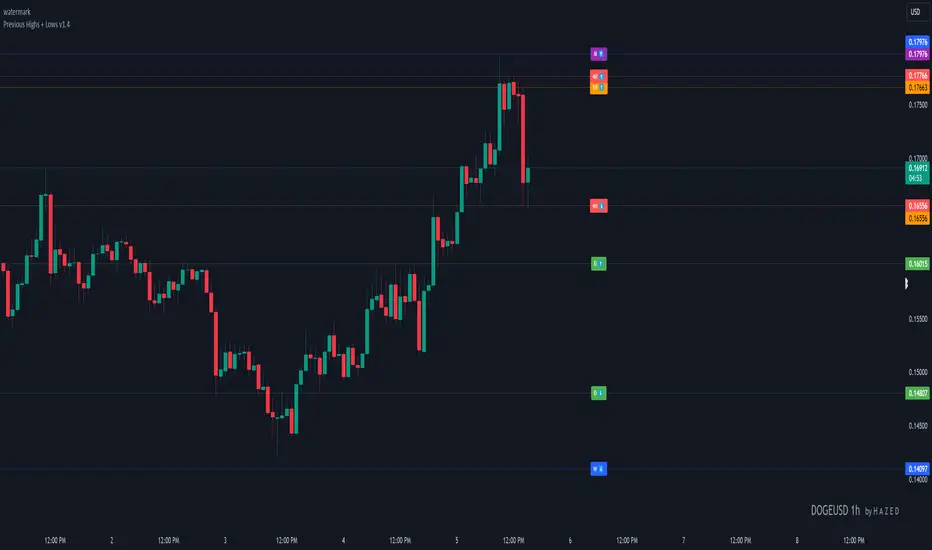
Previous Highs + Lows by HAZED📈 Introducing: Previous Highs + Lows by H A Z E D 📉
✨ Overview
Get a clear view of market levels with Previous Highs + Lows v1.0! This indicator lets you track critical previous highs and lows across multiple timeframes, marking them directly on your chart for an intuitive view of support and resistance zones. Whether you’re analyzing breakouts or looking for reversal levels, these indicators provide essential context to refine your trades.
🛠️ Key Features
Multiple Timeframes Supported
Toggle on previous highs and lows for daily, weekly, monthly, 4-hour, and 1-hour charts to match your analysis style.
Customizable Labels
Choose label sizes from “tiny” to “huge,” adjust the opacity to blend seamlessly with your chart, and customize text color for optimal readability.
Label Position Control
Avoid overlap with a flexible label offset feature, allowing for 10 adjustable increments to fit your preference and chart layout.
Clear Visual Cues
Labels use icons to differentiate high (⬆️) and low (⬇️) levels at a glance, providing a straightforward way to interpret key price areas.
Instant Alerts for Key Levels
Receive alerts when the price crosses over previous high levels, keeping you informed about potential breakout zones without constant chart-watching.
🚀 How to Use
Identify Key Levels: Quickly locate significant highs and lows from previous periods to define your support and resistance zones.
Set Alerts: Stay updated on market moves with built-in alerts when prices cross these critical levels.
Customize Your View: Use the various options to make this indicator uniquely yours – adjust label size, color, opacity, and position.
🔔 Why Use Previous Highs + Lows v1.0?
Enhanced visibility of critical levels saves you time by giving you a structured view of price action.
Customization features let you adapt the indicator to your personal style and chart setup.
Flexible alerts mean you can focus on other tasks without missing important price movements.
🔗 License: Mozilla Public License 2.0
© H A Z E D, 11/4/2024
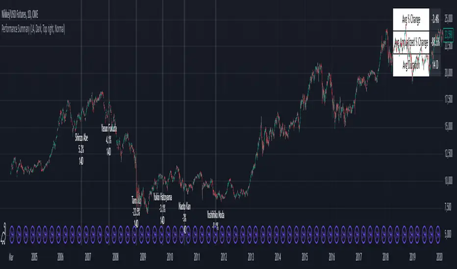
Performance Summary and Shading (Offset Version)Modified "Recession and Crisis Shading" Indicator by @haribotagada (Original Link: )
The updated indicator accepts a days offset (positive or negative) to calculate performance between the offset date and the input date.
Potential uses include identifying performance one week after company earnings or an FOMC meeting.
This feature simplifies input by enabling standardized offset dates, while still allowing flexibility to adjust ranges by overriding inputs as needed.
Summary of added features and indicator notes:
Inputs both positive and negative offset.
By default, the script calculates performance from the close of the input date to the close of the date at (input date + offset) for positive offsets, and from the close of (input date - offset) to the close of the input date for negative offsets. For example, with an input date of November 1, 2024, an offset of 7 calculates performance from the close on November 1 to the close on November 8, while an offset of -7 calculates from the close on October 25 to the close on November 1.
Allows user to perform the calculation using the open price on the input date instead of close price
The input format has been modified to allow overrides for the default duration, while retaining the original capabilities of the indicator.
The calculation shows both the average change and the average annualized change. For bar-wise calculations, annualization assumes 252 trading days per year. For date-wise calculations, it assumes 365 days for annualization.
Carries over all previous inputs to retain functionality of the previous script. Changes a few small settings:
Calculates start to end date performance by default instead of peak to trough performance.
Updates visuals of label text to make it easier to read and less transparent.
Changed stat box color scheme to make the text easier to read
Updated default input data to new format of input with offsets
Changed default duration statistic to number of days instead of number of bars with an option to select number of bars.
Potential Features to Add:
Import dataset from CSV files or by plugging into TradingView calendar
Example Input Datasets:
Recessions:
2020-02-01,COVID-19,59
2007-12-01,Subprime mortgages,547
2001-03-01,Dot-com,243
1990-07-01,Oil shock,243
1981-07-01,US unemployment,788
1980-01-01,Volker,182
1973-11-01,OPEC,485
Japan Revolving Door Elections
2006-09-26, Shinzo Abe
2007-09-26, Yasuo Fukuda
2008-09-24, Taro Aso
2009-09-16, Yukio Hatoyama
2010-07-08, Naoto Kan
2011-09-02, Yoshihiko Noda
Hope you find the modified indicator useful and let me know if you would like any features to be added!
ICT Open Range Gap & 1st FVG (fadi)In his 2024 mentorship program, ICT detailed how price action interacts with Open Range Gaps and the initial 1-minute Fair Value Gap following the market open at 9:30 AM.
What is an Open Range Gap?
An Open Range Gap occurs when the market opens at 9:30 AM at a higher or lower level compared to the previous day's close at 4:14 PM, primarily relevant in futures trading. According to ICT, there is a statistical probability of 70% that the price action will close 50% or more of the Open Range Gap within the first 30 minutes of trading (9:30 AM to 10:00 AM).
What is the First 1-Minute Fair Value Gap?
ICT places significant emphasis on the first 1-minute Fair Value Gap (FVG) that forms after the market opens at 9:30 AM. The FVG must occur at 9:31 AM or later to be considered valid. This gap often presents key opportunities for traders, as it represents a temporary imbalance between supply and demand that the market seeks to correct.
Understanding and leveraging these patterns can enhance trading strategies by offering insights into potential price movements shortly after market open.
ICT Open Range Gap & 1st FVG
This indicator is engineered to identify and highlight the Open Range Gaps and the first 1-minute Fair Value Gap. Furthermore, it functions across multiple timeframes, from seconds to hours, catering to various trading preferences. This flexibility is particularly beneficial for traders who favor higher timeframes or wish to observe these patterns' application at broader intervals.
Settings
The Open Range Gap indicator offers flexible display settings. It identifies the quadrants and provides optional color coding to distinguish them. Additionally, it tracks the "fill" level to visualize how far the price action has progressed into the gap, enhancing traders' ability to monitor and analyze price movements effectively. By default, the Open Range Gap will stop extending at 10:00 AM; however, there is an option to continue extending until the end of the trading day.
The 1st Fair Value Gap (FVG) can be viewed on any timeframe the indicator is active on, offering various styling options to match each trader's preferences. While the 1st FVG is particularly relevant to the day it is created, previous 1st FVGs within the same week may provide additional value. This indicator allows traders to extend Monday's 1st FVG, marking the first FVG of the week, or to extend all 1st FVGs throughout the week.

Indicator SELL UBScript Name: UB Sell Indicator based on 10Y Volume and Trend
Description: This indicator uses the 10-year interest rate (10Y1!) volume and price data to generate sell signals on the UB contract. When the 10Y1! volume exceeds a fixed threshold and the 10Y1! price is rising, a sell signal is issued to help traders anticipate bearish moves on the UB.
Features:
10Y1! Volume: Identifies periods of high volume.
10Y1! Price: Detects bullish trends in the 10Y1!.
Sell Signals: Displays red arrows to indicate selling opportunities on UB when conditions are met.
Visual Indicators: Colors and arrows for easy signal interpretation.
Parameters:
Fixed Volume Threshold: 114 (modifiable as needed).
Moving Average Period: 10 (to calculate the 10Y1! price trend).
Usage:
Watch for red arrows to identify selling opportunities on UB.
Combine with other analyses and indicators for a complete trading strategy.
Author: Jm Smeers
Publication Date: 26/10/2024

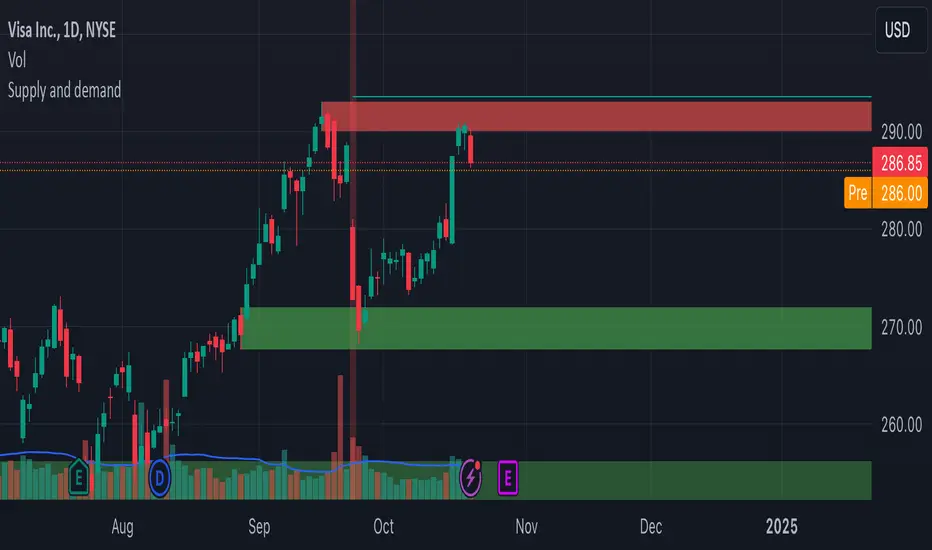
Supply and demandHi all!
This is my take on supply/demand. The gist is that it creates a zone if there is a big enough reaction. This is configurable in settings as "Minimum range (ATR factor)" (the Average True Length of length 14) that is the distance that the price must travel and "Reaction bars" that is the maximum number of bars that price must travel this distance. The zones that are shown are the ones that have a retest, break and retest or is unmitigated (untouched). If a zone is mitigated (entered) or broken it is temporarily hidden. For a zone to be created it needs to have this reaction and the previous bar does not.
So this script will show you zones that are fresh (unmitigated), retested or broken and retested. This means that the zones that are shown have "proven" that they are good zones through this. Basically it means that the script creates a bunch of zones and then picks the good once. This makes the script have some latency, but will hopefully give you good zones. A zone is completely removed if it's broken twice (it's okay if it's broken once and can still have a retest after it has flipped from previous supply (or resistance) into demand (or support)).
Here is a zone (the one that has the lowest opacity) that is broken and retested that could have resulted in a good long trade (the settings are default but has a stop in the beginning of 2024):
You have a setting to remove zones that are pierced (broken by price wicks). The following zone is pierced by price (in the beginning of May) that will not be shown after the start of May if you have "Pierced" checked (the indicator has default settings but a stop in the middle of April):
You have a trend section. Zones that create a reaction upwards can only be created if the trend is considered to be up, and vice versa. The options here are "SMA50" (the current price needs to be over the Simple Moving Average of length 50) and "SMA50, SMA200" (price needs to be over the Simple Moving Average of length 50 and the Simple Moving Average of length 50 needs to be over the Simple Moving Average of length 200). If these conditions are met the trend is considered to be up, otherwise it's down. You can disable this by choosing "No detection".
The zones that are shown also need to be within a limit (of the current price). This limit is 10 (factor of the Average True Range if length 14) by default. Set this to 0 to deactivate. This is useful for not showing zones that are far away from current price and therefore unlikely to be interacted with.
You can stop the calculation of zones (through the "Stop" value in the settings). This is useful to see if previous zones were any good. I used it in my testing of the script but left it because it can be nice to have.
The zones created by the script have different transparency based upon the zone's interaction. The clearest zones are the ones that are unmitigated, the second clearest ones are the ones having a retest and lastly the zones which are most unclear are the ones having a break and then a retest.
You can see the concept of this script to be a mix of supply/demand and support/resistance, having zones being unmitigated (untouched) as the most important but also show the zones having an interaction (in the form of a retest or a break and retest).
This is from a previous supply (or resistance) zone that has flipped into demand (or support) and has shown to be a good zone through a retest followed by a rally (default settings):
This zone has multiple retest and then rallies that could have given a good long trades (it has the default settings but a "Stop" time at 2022-01-14):
TODO:
- Create zones based on pivots
- Handle overlapping zones
- Incorporate volume in the creation and/or interaction with zones
- Add alerts
- Add ability to set maximum zone width
- Add ability to set the maximum number of retest bars
- ...?
The example for this publication has the default settings bit a "Stop" and a tighter "Limit" of 4.
I hope this explanation makes sense, let me know otherwise. Also let me know if you have any suggestions on improvements.
Best of trading luck!
ATR Trailing Stop by tactical trade 22 Oct 2024Description:
The ATR Dual Trailing Stop indicator is a versatile and powerful tool designed to help traders visualize dynamic support and resistance levels based on the Average True Range (ATR). This indicator plots two separate ATR-based trailing stops with customizable settings, providing a comprehensive view of potential market reversals and trend strength.
Key features:
Two ATR Trailing Stops: The first stop uses customizable ATR settings (default: 10-period ATR with a 3x multiplier), while the second stop uses an alternate configuration (default: 21-period ATR with a 7x multiplier).
Multi-Timeframe ATR Calculation: Regardless of the chart's time frame, the ATR is calculated based on a user-selected time frame (e.g., daily), allowing for consistent stop-loss levels even in lower time frames like 5-minute or 15-minute charts.
Visual Cues: The indicator clearly plots two trailing stop lines in different colors, making it easy to track the market’s volatility-based support and resistance areas.
No Buy/Sell Signals: This is purely a trailing stop indicator with no embedded buy/sell signals, giving traders the flexibility to use it with their preferred entry/exit strategies.
This indicator is especially useful in highly volatile markets where precise trailing stop levels are essential for managing risk and maximizing profit potential. The dual ATR configuration helps traders adapt to changing market conditions by providing two levels of stop placement: a shorter-term and a longer-term trailing stop.

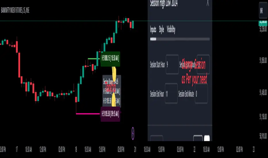
Session High Low 2024
Overview of the Code:
Input for Session Times:
You set up inputs for the start and end times of the trading session, allowing you to customize them as needed.
Time Range Function:
A function isTimeInRange checks whether the current time falls within the specified session start and end times.
initialize High and Low:
indicator initialize session high, low, and their corresponding labels and lines.
Tracking Session High and Low:
Within the specified time range, continuously update session1High and session1Low based on the highest and lowest prices encountered.
Time of Session High/Low:
The High_Time and Low_Time are tracked using the ta.valuewhen() function to capture the exact times when the session high and low occur.
Notes Creation:
You format the high and low values along with their timestamps to create notes that will be displayed alongside the lines.
Drawing Lines and Labels:
After the session ends, you check if there is a new session high or low and draw lines and labels accordingly. If a line or label already exists, you delete it before drawing a new one.
Resetting for Next Session:
At the end of the session, the high and low values are reset for the next session.
Suggestions for Improvement:
Dynamic Line Extensions:
Clear Variable Names Used in Code:
Consider using more descriptive names for variables like Entry_Point and SL_Point to make the code easier to understand.
Commenting:
Although the code is well-commented, always ensure the comments explain the "why" behind the code rather than just the "what."
Example Output:
The output will show the highest and lowest prices during the specified session times and the times they occurred formatted correctly. This output is useful for quick reference during trading and aids in making informed decisions.
Added functionality tool tip Note:
Added a tooltip Note to Get All information of Session High Low & Range.
If you need further modifications, enhancements, or specific functionalities added to this script, please let me know!
Commitment of Trader %R StrategyThis Pine Script strategy utilizes the Commitment of Traders (COT) data to inform trading decisions based on the Williams %R indicator. The script operates in TradingView and includes various functionalities that allow users to customize their trading parameters.
Here’s a breakdown of its key components:
COT Data Import:
The script imports the COT library from TradingView to access historical COT data related to different trader groups (commercial hedgers, large traders, and small traders).
User Inputs:
COT data selection mode (e.g., Auto, Root, Base currency).
Whether to include futures, options, or both.
The trader group to analyze.
The lookback period for calculating the Williams %R.
Upper and lower thresholds for triggering trades.
An option to enable or disable a Simple Moving Average (SMA) filter.
Williams %R Calculation: The script calculates the Williams %R value, which is a momentum indicator that measures overbought or oversold levels based on the highest and lowest prices over a specified period.
SMA Filter: An optional SMA filter allows users to limit trades to conditions where the price is above or below the SMA, depending on the configuration.
Trade Logic: The strategy enters long positions when the Williams %R value exceeds the upper threshold and exits when the value falls below it. Conversely, it enters short positions when the Williams %R value is below the lower threshold and exits when the value rises above it.
Visual Elements: The script visually indicates the Williams %R values and thresholds on the chart, with the option to plot the SMA if enabled.
Commitment of Traders (COT) Data
The COT report is a weekly publication by the Commodity Futures Trading Commission (CFTC) that provides a breakdown of open interest positions held by different types of traders in the U.S. futures markets. It is widely used by traders and analysts to gauge market sentiment and potential price movements.
Data Collection: The COT data is collected from futures commission merchants and is published every Friday, reflecting positions as of the previous Tuesday. The report categorizes traders into three main groups:
Commercial Traders: These are typically hedgers (like producers and processors) who use futures to mitigate risk.
Non-Commercial Traders: Often referred to as speculators, these traders do not have a commercial interest in the underlying commodity but seek to profit from price changes.
Non-reportable Positions: Small traders who do not meet the reporting threshold set by the CFTC.
Interpretation:
Market Sentiment: By analyzing the positions of different trader groups, market participants can gauge sentiment. For instance, if commercial traders are heavily short, it may suggest they expect prices to decline.
Extreme Positions: Some traders look for extreme positions among non-commercial traders as potential reversal signals. For example, if speculators are overwhelmingly long, it might indicate an overbought condition.
Statistical Insights: COT data is often used in conjunction with technical analysis to inform trading decisions. Studies have shown that analyzing COT data can provide valuable insights into future price movements (Lund, 2018; Hurst et al., 2017).
Scientific References
Lund, J. (2018). Understanding the COT Report: An Analysis of Speculative Trading Strategies.
Journal of Derivatives and Hedge Funds, 24(1), 41-52. DOI:10.1057/s41260-018-00107-3
Hurst, B., O'Neill, R., & Roulston, M. (2017). The Impact of COT Reports on Futures Market Prices: An Empirical Analysis. Journal of Futures Markets, 37(8), 763-785.
DOI:10.1002/fut.21849
Commodity Futures Trading Commission (CFTC). (2024). Commitment of Traders. Retrieved from CFTC Official Website.
