PatternTransitionTablesPatternTransitionTables Library
🌸 Part of GoemonYae Trading System (GYTS) 🌸
🌸 --------- 1. INTRODUCTION --------- 🌸
💮 Overview
This library provides precomputed state transition tables to enable ultra-efficient, O(1) computation of Ordinal Patterns. It is designed specifically to support high-performance indicators calculating Permutation Entropy and related complexity measures.
💮 The Problem & Solution
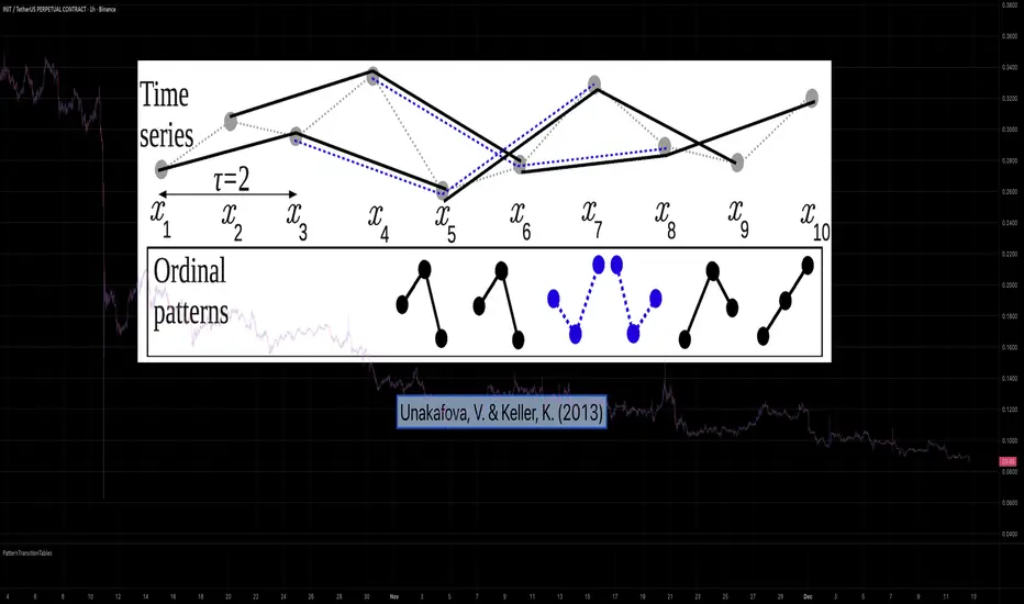
Calculating Permutation Entropy, as introduced by Bandt and Pompe (2002), typically requires computing ordinal patterns within a sliding window at every time step. The standard successive-pattern method (Equations 2+3 in the paper) requires ≤ 4d-1 operations per update.
Unakafova and Keller (2013) demonstrated that successive ordinal patterns "overlap" significantly. By knowing the current pattern index and the relative rank (position l) of just the single new data point, the next pattern index can be determined via a precomputed look-up table. Computing l still requires d comparisons, but the table lookup itself is O(1), eliminating the need for d multiplications and d additions. This reduces total operations from ≤ 4d-1 to ≤ 2d per update (Table 4). This library contains these precomputed tables for orders d = 2 through d = 5.
🌸 --------- 2. THEORETICAL BACKGROUND --------- 🌸
💮 Permutation Entropy
Bandt, C., & Pompe, B. (2002). Permutation entropy: A natural complexity measure for time series.
doi.org
This concept quantifies the complexity of a system by comparing the order of neighbouring values rather than their magnitudes. It is robust against noise and non-linear distortions, making it ideal for financial time series analysis.
💮 Efficient Computation
Unakafova, V. A., & Keller, K. (2013). Efficiently Measuring Complexity on the Basis of Real-World Data.
doi.org
This library implements the transition function φ_d(n, l) described in Equation 5 of the paper. It maps a current pattern index (n) and the position of the new value (l) to the successor pattern, reducing the complexity of updates to constant time O(1).
🌸 --------- 3. LIBRARY FUNCTIONALITY --------- 🌸
💮 Data Structure
The library stores transition matrices as flattened 1D integer arrays. These tables are mathematically rigorous representations of the factorial number system used to enumerate permutations.
💮 Core Function: get_successor()
This is the primary interface for the library for direct pattern updates.
• Input: The current pattern index and the rank position of the incoming price data.
• Process: Routes the request to the specific transition table for the chosen order (d=2 to d=5).
• Output: The integer index of the next ordinal pattern.
💮 Table Access: get_table()
This function returns the entire flattened transition table for a specified dimension. This enables local caching of the table (e.g. in an indicator's init() method), avoiding the overhead of repeated library calls during the calculation loop.
💮 Supported Orders & Terminology
The parameter d is the order of ordinal patterns (following Bandt & Pompe 2002). Each pattern of order d contains (d+1) data points, yielding (d+1)! unique patterns:
• d=2: 3 points → 6 unique patterns, 3 successor positions
• d=3: 4 points → 24 unique patterns, 4 successor positions
• d=4: 5 points → 120 unique patterns, 5 successor positions
• d=5: 6 points → 720 unique patterns, 6 successor positions
Note: d=6 is not implemented. The resulting code size (approx. 191k tokens) exceeds the Pine Script limit of 100k tokens (as of 2025-12).
Statistics
LuxyEnergyIndexThe Luxy Energy Index (LEI) library provides functions to measure price movement exhaustion by analyzing three dimensions: Extension (distance from fair value), Velocity (speed of movement), and Volume (confirmation level).
LEI answers a different question than traditional momentum indicators: instead of "how far has price gone?" (like RSI), LEI asks "how tired is this move?"
This library allows Pine Script developers to integrate LEI calculations into their own indicators and strategies.
How to Import
//@version=6
indicator("My Indicator")
import OrenLuxy/LuxyEnergyIndex/1 as LEI
Main Functions
`lei(src)` → float
Returns the LEI value on a 0-100 scale.
src (optional): Price source, default is `close`
Returns : LEI value (0-100) or `na` if insufficient data (first 50 bars)
leiValue = LEI.lei()
leiValue = LEI.lei(hlc3) // custom source
`leiDetailed(src)` → tuple
Returns LEI with all component values for detailed analysis.
= LEI.leiDetailed()
Returns:
`lei` - Final LEI value (0-100)
`extension` - Distance from VWAP in ATR units
`velocity` - 5-bar price change in ATR units
`volumeZ` - Volume Z-Score
`volumeModifier` - Applied modifier (1.0 = neutral)
`vwap` - VWAP value used
Component Functions
| Function | Description | Returns |
|-----------------------------------|---------------------------------|---------------|
| `calcExtension(src, vwap)` | Distance from VWAP / ATR | float |
| `calcVelocity(src)` | 5-bar price change / ATR | float |
| `calcVolumeZ()` | Volume Z-Score | float |
| `calcVolumeModifier(volZ)` | Volume modifier | float (≥1.0) |
| `getVWAP()` | Auto-detects asset type | float |
Signal Functions
| Function | Description | Returns |
|---------------------------------------------|----------------------------------|-----------|
| `isExhausted(lei, threshold)` | LEI ≥ threshold (default 70) | bool |
| `isSafe(lei, threshold)` | LEI ≤ threshold (default 30) | bool |
| `crossedExhaustion(lei, threshold)` | Crossed into exhaustion | bool |
| `crossedSafe(lei, threshold)` | Crossed into safe zone | bool |
Utility Functions
| Function | Description | Returns |
|----------------------------|-------------------------|-----------|
| `getZone(lei)` | Zone name | string |
| `getColor(lei)` | Recommended color | color |
| `hasEnoughHistory()` | Data check | bool |
| `minBarsRequired()` | Required bars | int (50) |
| `version()` | Library version | string |
Interpretation Guide
| LEI Range | Zone | Meaning |
|-------------|--------------|--------------------------------------------------|
| 0-30 | Safe | Low exhaustion, move may continue |
| 30-50 | Caution | Moderate exhaustion |
| 50-70 | Warning | Elevated exhaustion |
| 70-100 | Exhaustion | High exhaustion, increased reversal risk |
Example: Basic Usage
//@version=6
indicator("LEI Example", overlay=false)
import OrenLuxy/LuxyEnergyIndex/1 as LEI
// Get LEI value
leiValue = LEI.lei()
// Plot with dynamic color
plot(leiValue, "LEI", LEI.getColor(leiValue), 2)
// Reference lines
hline(70, "High", color.red)
hline(30, "Low", color.green)
// Alert on exhaustion
if LEI.crossedExhaustion(leiValue) and barstate.isconfirmed
alert("LEI crossed into exhaustion zone")
Technical Details
Fixed Parameters (by design):
Velocity Period: 5 bars
Volume Period: 20 bars
Z-Score Period: 50 bars
ATR Period: 14
Extension/Velocity Weights: 50/50
Asset Support:
Stocks/Forex: Uses Session VWAP (daily reset)
Crypto: Uses Rolling VWAP (50-bar window) - auto-detected
Edge Cases:
Returns `na` until 50 bars of history
Zero volume: Volume modifier defaults to 1.0 (neutral)
Credits and Acknowledgments
This library builds upon established technical analysis concepts:
VWAP - Industry standard volume-weighted price measure
ATR by J. Welles Wilder Jr. (1978) - Volatility normalization
Z-Score - Statistical normalization method
Volume analysis principles from Volume Spread Analysis (VSA) methodology
Disclaimer
This library is provided for **educational and informational purposes only**. It does not constitute financial advice. Past performance does not guarantee future results. The exhaustion readings are probabilistic indicators, not guarantees of price reversal. Always conduct your own research and use proper risk management when trading.

KernelFunctionsLibrary "KernelFunctions"
This library provides non-repainting kernel functions for Nadaraya-Watson estimator implementations. This allows for easy substition/comparison of different kernel functions for one another in indicators. Furthermore, kernels can easily be combined with other kernels to create newer, more customized kernels.
rationalQuadratic(_src, _lookback, _relativeWeight, startAtBar)
Rational Quadratic Kernel - An infinite sum of Gaussian Kernels of different length scales.
Parameters:
_src (float) : The source series.
_lookback (simple int) : The number of bars used for the estimation. This is a sliding value that represents the most recent historical bars.
_relativeWeight (simple float) : Relative weighting of time frames. Smaller values resut in a more stretched out curve and larger values will result in a more wiggly curve. As this value approaches zero, the longer time frames will exert more influence on the estimation. As this value approaches infinity, the behavior of the Rational Quadratic Kernel will become identical to the Gaussian kernel.
startAtBar (simple int)
Returns: yhat The estimated values according to the Rational Quadratic Kernel.
gaussian(_src, _lookback, startAtBar)
Gaussian Kernel - A weighted average of the source series. The weights are determined by the Radial Basis Function (RBF).
Parameters:
_src (float) : The source series.
_lookback (simple int) : The number of bars used for the estimation. This is a sliding value that represents the most recent historical bars.
startAtBar (simple int)
Returns: yhat The estimated values according to the Gaussian Kernel.
periodic(_src, _lookback, _period, startAtBar)
Periodic Kernel - The periodic kernel (derived by David Mackay) allows one to model functions which repeat themselves exactly.
Parameters:
_src (float) : The source series.
_lookback (simple int) : The number of bars used for the estimation. This is a sliding value that represents the most recent historical bars.
_period (simple int) : The distance between repititions of the function.
startAtBar (simple int)
Returns: yhat The estimated values according to the Periodic Kernel.
locallyPeriodic(_src, _lookback, _period, startAtBar)
Locally Periodic Kernel - The locally periodic kernel is a periodic function that slowly varies with time. It is the product of the Periodic Kernel and the Gaussian Kernel.
Parameters:
_src (float) : The source series.
_lookback (simple int) : The number of bars used for the estimation. This is a sliding value that represents the most recent historical bars.
_period (simple int) : The distance between repititions of the function.
startAtBar (simple int)
Returns: yhat The estimated values according to the Locally Periodic Kernel.

machine_learningLibrary "machine_learning"
euclidean(a, b)
Parameters:
a (array)
b (array)
manhattan(a, b)
Parameters:
a (array)
b (array)
cosine_similarity(a, b)
Parameters:
a (array)
b (array)
cosine_distance(a, b)
Parameters:
a (array)
b (array)
chebyshev(a, b)
Parameters:
a (array)
b (array)
minkowski(a, b, p)
Parameters:
a (array)
b (array)
p (float)
dot_product(a, b)
Parameters:
a (array)
b (array)
vector_norm(arr, p)
Parameters:
arr (array)
p (float)
sigmoid(x)
Parameters:
x (float)
sigmoid_derivative(x)
Parameters:
x (float)
tanh_derivative(x)
Parameters:
x (float)
relu(x)
Parameters:
x (float)
relu_derivative(x)
Parameters:
x (float)
leaky_relu(x, alpha)
Parameters:
x (float)
alpha (float)
leaky_relu_derivative(x, alpha)
Parameters:
x (float)
alpha (float)
elu(x, alpha)
Parameters:
x (float)
alpha (float)
gelu(x)
Parameters:
x (float)
swish(x, beta)
Parameters:
x (float)
beta (float)
softmax(arr)
Parameters:
arr (array)
apply_activation(arr, activation_type, alpha)
Parameters:
arr (array)
activation_type (string)
alpha (float)
normalize_minmax(arr, min_val, max_val)
Parameters:
arr (array)
min_val (float)
max_val (float)
normalize_zscore(arr, mean_val, std_val)
Parameters:
arr (array)
mean_val (float)
std_val (float)
normalize_matrix_cols(m)
Parameters:
m (matrix)
scaler_fit(arr, method)
Parameters:
arr (array)
method (string)
scaler_fit_matrix(m, method)
Parameters:
m (matrix)
method (string)
scaler_transform(scaler, arr)
Parameters:
scaler (ml_scaler)
arr (array)
scaler_transform_matrix(scaler, m)
Parameters:
scaler (ml_scaler)
m (matrix)
clip(x, lo, hi)
Parameters:
x (float)
lo (float)
hi (float)
clip_array(arr, lo, hi)
Parameters:
arr (array)
lo (float)
hi (float)
loss_mse(predicted, actual)
Parameters:
predicted (array)
actual (array)
loss_rmse(predicted, actual)
Parameters:
predicted (array)
actual (array)
loss_mae(predicted, actual)
Parameters:
predicted (array)
actual (array)
loss_binary_crossentropy(predicted, actual)
Parameters:
predicted (array)
actual (array)
loss_huber(predicted, actual, delta)
Parameters:
predicted (array)
actual (array)
delta (float)
gradient_step(weights, gradients, lr)
Parameters:
weights (array)
gradients (array)
lr (float)
adam_step(weights, gradients, m, v, lr, beta1, beta2, t, epsilon)
Parameters:
weights (array)
gradients (array)
m (array)
v (array)
lr (float)
beta1 (float)
beta2 (float)
t (int)
epsilon (float)
clip_gradients(gradients, max_norm)
Parameters:
gradients (array)
max_norm (float)
lr_decay(initial_lr, decay_rate, step)
Parameters:
initial_lr (float)
decay_rate (float)
step (int)
lr_cosine_annealing(initial_lr, min_lr, step, total_steps)
Parameters:
initial_lr (float)
min_lr (float)
step (int)
total_steps (int)
knn_create(k, distance_type)
Parameters:
k (int)
distance_type (string)
knn_fit(model, X, y)
Parameters:
model (ml_knn)
X (matrix)
y (array)
knn_predict(model, x)
Parameters:
model (ml_knn)
x (array)
knn_predict_proba(model, x)
Parameters:
model (ml_knn)
x (array)
knn_batch_predict(model, X)
Parameters:
model (ml_knn)
X (matrix)
linreg_fit(X, y)
Parameters:
X (matrix)
y (array)
ridge_fit(X, y, lambda)
Parameters:
X (matrix)
y (array)
lambda (float)
linreg_predict(model, x)
Parameters:
model (ml_linreg)
x (array)
linreg_predict_batch(model, X)
Parameters:
model (ml_linreg)
X (matrix)
linreg_score(model, X, y)
Parameters:
model (ml_linreg)
X (matrix)
y (array)
logreg_create(n_features, learning_rate, iterations)
Parameters:
n_features (int)
learning_rate (float)
iterations (int)
logreg_fit(model, X, y)
Parameters:
model (ml_logreg)
X (matrix)
y (array)
logreg_predict_proba(model, x)
Parameters:
model (ml_logreg)
x (array)
logreg_predict(model, x, threshold)
Parameters:
model (ml_logreg)
x (array)
threshold (float)
logreg_batch_predict(model, X, threshold)
Parameters:
model (ml_logreg)
X (matrix)
threshold (float)
nb_create(n_classes)
Parameters:
n_classes (int)
nb_fit(model, X, y)
Parameters:
model (ml_nb)
X (matrix)
y (array)
nb_predict_proba(model, x)
Parameters:
model (ml_nb)
x (array)
nb_predict(model, x)
Parameters:
model (ml_nb)
x (array)
nn_create(layers, activation)
Parameters:
layers (array)
activation (string)
nn_forward(model, x)
Parameters:
model (ml_nn)
x (array)
nn_predict_class(model, x)
Parameters:
model (ml_nn)
x (array)
accuracy(y_true, y_pred)
Parameters:
y_true (array)
y_pred (array)
precision(y_true, y_pred, positive_class)
Parameters:
y_true (array)
y_pred (array)
positive_class (int)
recall(y_true, y_pred, positive_class)
Parameters:
y_true (array)
y_pred (array)
positive_class (int)
f1_score(y_true, y_pred, positive_class)
Parameters:
y_true (array)
y_pred (array)
positive_class (int)
r_squared(y_true, y_pred)
Parameters:
y_true (array)
y_pred (array)
mse(y_true, y_pred)
Parameters:
y_true (array)
y_pred (array)
rmse(y_true, y_pred)
Parameters:
y_true (array)
y_pred (array)
mae(y_true, y_pred)
Parameters:
y_true (array)
y_pred (array)
confusion_matrix(y_true, y_pred, n_classes)
Parameters:
y_true (array)
y_pred (array)
n_classes (int)
sliding_window(data, window_size)
Parameters:
data (array)
window_size (int)
train_test_split(X, y, test_ratio)
Parameters:
X (matrix)
y (array)
test_ratio (float)
create_binary_labels(data, threshold)
Parameters:
data (array)
threshold (float)
lag_matrix(data, n_lags)
Parameters:
data (array)
n_lags (int)
signal_to_position(prediction, threshold_long, threshold_short)
Parameters:
prediction (float)
threshold_long (float)
threshold_short (float)
confidence_sizing(probability, max_size, min_confidence)
Parameters:
probability (float)
max_size (float)
min_confidence (float)
kelly_sizing(win_rate, avg_win, avg_loss, max_fraction)
Parameters:
win_rate (float)
avg_win (float)
avg_loss (float)
max_fraction (float)
sharpe_ratio(returns, risk_free_rate)
Parameters:
returns (array)
risk_free_rate (float)
sortino_ratio(returns, risk_free_rate)
Parameters:
returns (array)
risk_free_rate (float)
max_drawdown(equity)
Parameters:
equity (array)
atr_stop_loss(entry_price, atr, multiplier, is_long)
Parameters:
entry_price (float)
atr (float)
multiplier (float)
is_long (bool)
risk_reward_take_profit(entry_price, stop_loss, ratio)
Parameters:
entry_price (float)
stop_loss (float)
ratio (float)
ensemble_vote(predictions)
Parameters:
predictions (array)
ensemble_weighted_average(predictions, weights)
Parameters:
predictions (array)
weights (array)
smooth_prediction(current, previous, alpha)
Parameters:
current (float)
previous (float)
alpha (float)
regime_classifier(volatility, trend_strength, vol_threshold, trend_threshold)
Parameters:
volatility (float)
trend_strength (float)
vol_threshold (float)
trend_threshold (float)
ml_knn
Fields:
k (series int)
distance_type (series string)
X_train (matrix)
y_train (array)
ml_linreg
Fields:
coefficients (array)
intercept (series float)
lambda (series float)
ml_logreg
Fields:
weights (array)
bias (series float)
learning_rate (series float)
iterations (series int)
ml_nn
Fields:
layers (array)
weights (matrix)
biases (array)
weight_offsets (array)
bias_offsets (array)
activation (series string)
ml_nb
Fields:
class_priors (array)
means (matrix)
variances (matrix)
n_classes (series int)
ml_scaler
Fields:
min_vals (array)
max_vals (array)
means (array)
stds (array)
method (series string)
ml_train_result
Fields:
loss_history (array)
final_loss (series float)
converged (series bool)
iterations_run (series int)
ml_prediction
Fields:
class_label (series int)
probability (series float)
probabilities (array)
value (series float)

CEDEARDataLibrary "CEDEARData"
getUnderlying(cedearTicker)
Parameters:
cedearTicker (simple string)
getRatio(cedearTicker)
Parameters:
cedearTicker (simple string)
getCurrency(cedearTicker)
Parameters:
cedearTicker (simple string)
isValidCedear(cedearTicker)
Parameters:
cedearTicker (simple string)

RLSR logreg_support_libLibrary "logreg_support_lib"
sigmoid(z)
Parameters:
z (float)
prng01(seed1, seed2)
Parameters:
seed1 (float)
seed2 (float)
normalize(value, minval, maxval)
Parameters:
value (float)
minval (float)
maxval (float)
calcpercentilefast(arr, percentile)
Parameters:
arr (array)
percentile (float)
calcpercentile_series_sampled(s, length, percentile, stride)
Parameters:
s (float)
length (int)
percentile (float)
stride (int)
calcRangeWithLog(value, minval, maxval, uselog)
Parameters:
value (float)
minval (float)
maxval (float)
uselog (bool)
calcMomentumAdvanced(src, length, momType)
Parameters:
src (float)
length (simple int)
momType (string)
normalizeMomentumByType(rawMom, momType, momMin, momMax, momNorm)
Parameters:
rawMom (float)
momType (string)
momMin (float)
momMax (float)
momNorm (float)
normalizeMomentumByTypeExt(rawMom, momType, momMin, momMax, momNorm, bouncingdecay)
Parameters:
rawMom (float)
momType (string)
momMin (float)
momMax (float)
momNorm (float)
bouncingdecay (float)
calcrollingstddev(src, length)
Parameters:
src (float)
length (int)
addlog(buffer, level, msg)
Parameters:
buffer (string)
level (string)
msg (string)
calcfeaturecorrelation(x1, x2)
Parameters:
x1 (array)
x2 (array)
calcnoiseratio(src, lookback)
Parameters:
src (float)
lookback (int)
calccompatibilityscore(x1, x2)
Parameters:
x1 (array)
x2 (array)
getfuturereturn(offset, returnlookback)
Parameters:
offset (int)
returnlookback (int)
calculatema(source, length, matype)
Parameters:
source (float)
length (simple int)
matype (string)
adaptive_trigger_for_source(src, enabled, freeze, lookback, threshold, volahistory)
Parameters:
src (float)
enabled (bool)
freeze (bool)
lookback (int)
threshold (float)
volahistory (array)
checkadaptivetrigger5(s1, enabled1, freeze1, hist1, s2, enabled2, freeze2, hist2, s3, enabled3, freeze3, hist3, s4, enabled4, freeze4, hist4, s5, enabled5, freeze5, hist5, lookback, threshold)
Parameters:
s1 (float)
enabled1 (bool)
freeze1 (bool)
hist1 (array)
s2 (float)
enabled2 (bool)
freeze2 (bool)
hist2 (array)
s3 (float)
enabled3 (bool)
freeze3 (bool)
hist3 (array)
s4 (float)
enabled4 (bool)
freeze4 (bool)
hist4 (array)
s5 (float)
enabled5 (bool)
freeze5 (bool)
hist5 (array)
lookback (int)
threshold (float)
ring_start_index(rb_write_idx, rb_count, rb_cap)
Parameters:
rb_write_idx (int)
rb_count (int)
rb_cap (int)

reversalLibrary "reversals"
psar(af_start, af_increment, af_max)
Calculates Parabolic Stop And Reverse (SAR)
Parameters:
af_start (simple float) : Initial acceleration factor (Wilder's original: 0.02)
af_increment (simple float) : Acceleration factor increment per new extreme (Wilder's original: 0.02)
af_max (simple float) : Maximum acceleration factor (Wilder's original: 0.20)
Returns: SAR value (stop level for current trend)
fractals()
Detects Williams Fractal patterns (5-bar pattern)
Returns: Tuple with fractal values (na if no fractal)
swings(lookback, source_high, source_low)
Detects swing highs and swing lows using lookback period
Parameters:
lookback (simple int) : Number of bars on each side to confirm swing point
source_high (float) : Price series for swing high detection (typically high)
source_low (float) : Price series for swing low detection (typically low)
Returns: Tuple with swing point values (na if no swing)
pivot(tf)
Calculates classic/standard/floor pivot points
Parameters:
tf (simple string) : Timeframe for pivot calculation ("D", "W", "M")
Returns: Tuple with pivot levels
pivotcam(tf)
Calculates Camarilla pivot points with 8 levels for short-term trading
Parameters:
tf (simple string) : Timeframe for pivot calculation ("D", "W", "M")
Returns: Tuple with pivot levels
pivotdem(tf)
Calculates d-mark pivot points with conditional open/close logic
Parameters:
tf (simple string) : Timeframe for pivot calculation ("D", "W", "M")
Returns: Tuple with pivot levels (only 3 levels)
pivotext(tf)
Calculates extended traditional pivot points with R4-R5 and S4-S5 levels
Parameters:
tf (simple string) : Timeframe for pivot calculation ("D", "W", "M")
Returns: Tuple with pivot levels
pivotfib(tf)
Calculates Fibonacci pivot points using Fibonacci ratios
Parameters:
tf (simple string) : Timeframe for pivot calculation ("D", "W", "M")
Returns: Tuple with pivot levels
pivotwood(tf)
Calculates Woodie's pivot points with weighted closing price
Parameters:
tf (simple string) : Timeframe for pivot calculation ("D", "W", "M")
Returns: Tuple with pivot levels

LapseBacktestingTableLibrary "LapseBacktestingMetrics"
This library provides a robust set of quantitative backtesting and performance evaluation functions for Pine Script strategies. It’s designed to help traders, quants, and developers assess risk, return, and robustness through detailed statistical metrics — including Sharpe, Sortino, Omega, drawdowns, and trade efficiency.
Built to enhance any trading strategy’s evaluation framework, this library allows you to visualize performance with the quantlapseTable() function, producing an interactive on-chart performance table.
Credit to EliCobra and BikeLife76 for original concept inspiration.
curve(disp_ind)
Retrieves a selected performance curve of your strategy.
Parameters:
disp_ind (simple string): Type of curve to plot. Options include "Equity", "Open Profit", "Net Profit", "Gross Profit".
Returns: (float) Corresponding performance curve value.
cleaner(disp_ind, plot)
Filters and displays selected strategy plots for clean visualization.
Parameters:
disp_ind (simple string): Type of display.
plot (simple float): Strategy plot variable.
Returns: (float) Filtered plot value.
maxEquityDrawDown()
Calculates the maximum equity drawdown during the strategy’s lifecycle.
Returns: (float) Maximum equity drawdown percentage.
maxTradeDrawDown()
Computes the worst intra-trade drawdown among all closed trades.
Returns: (float) Maximum intra-trade drawdown percentage.
consecutive_wins()
Finds the highest number of consecutive winning trades.
Returns: (int) Maximum consecutive wins.
consecutive_losses()
Finds the highest number of consecutive losing trades.
Returns: (int) Maximum consecutive losses.
no_position()
Counts the maximum consecutive bars where no position was held.
Returns: (int) Maximum flat days count.
long_profit()
Calculates total profit generated by long positions as a percentage of initial capital.
Returns: (float) Total long profit %.
short_profit()
Calculates total profit generated by short positions as a percentage of initial capital.
Returns: (float) Total short profit %.
prev_month()
Measures the previous month’s profit or loss based on equity change.
Returns: (float) Monthly equity delta.
w_months()
Counts the number of profitable months in the backtest.
Returns: (int) Total winning months.
l_months()
Counts the number of losing months in the backtest.
Returns: (int) Total losing months.
checktf()
Returns the time-adjusted scaling factor used in Sharpe and Sortino ratio calculations based on chart timeframe.
Returns: (float) Annualization multiplier.
stat_calc()
Performs complete statistical computation including drawdowns, Sharpe, Sortino, Omega, trade stats, and profit ratios.
Returns: (array)
.
f_colors(x, nv)
Generates a color gradient for performance values, supporting dynamic table visualization.
Parameters:
x (simple string): Metric label name.
nv (simple float): Metric numerical value.
Returns: (color) Gradient color value for table background.
quantlapseTable(option, position)
Displays an interactive Performance Table summarizing all major backtesting metrics.
Includes Sharpe, Sortino, Omega, Profit Factor, drawdowns, profitability %, and trade statistics.
Parameters:
option (simple string): Table type — "Full", "Simple", or "None".
position (simple string): Table position — "Top Left", "Middle Right", "Bottom Left", etc.
Returns: (table) On-chart performance visualization table.
This library empowers advanced quantitative evaluation directly within Pine Script®, ideal for strategy developers seeking deeper performance diagnostics and intuitive on-chart metrics.

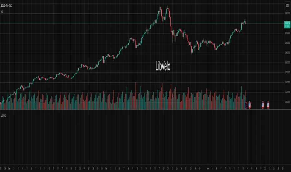
LibVeloLibrary "LibVelo"
This library provides a sophisticated framework for **Velocity
Profile (Flow Rate)** analysis. It measures the physical
speed of trading at specific price levels by relating volume
to the time spent at those levels.
## Core Concept: Market Velocity
Unlike Volume Profiles, which only answer "how much" traded,
Velocity Profiles answer "how fast" it traded.
It is calculated as:
`Velocity = Volume / Duration`
This metric (contracts per second) reveals hidden market
dynamics invisible to pure Volume or TPO profiles:
1. **High Velocity (Fast Flow):**
* **Aggression:** Initiative buyers/sellers hitting market
orders rapidly.
* **Liquidity Vacuum:** Price slips through a level because
order book depth is thin (low resistance).
2. **Low Velocity (Slow Flow):**
* **Absorption:** High volume but very slow price movement.
Indicates massive passive limit orders ("Icebergs").
* **Apathy:** Little volume over a long time. Lack of
interest from major participants.
## Architecture: Triple-Engine Composition
To ensure maximum performance while offering full statistical
depth for all metrics, this library utilises **object
composition** with a lazy evaluation strategy:
#### Engine A: The Master (`vpVol`)
* **Role:** Standard Volume Profile.
* **Purpose:** Maintains the "ground truth" of volume distribution,
price buckets, and ranges.
#### Engine B: The Time Container (`vpTime`)
* **Role:** specialized container for time duration (in ms).
* **Hack:** It repurposes standard volume arrays (specifically
`aBuy`) to accumulate time duration for each bucket.
#### Engine C: The Calculator (`vpVelo`)
* **Role:** Temporary scratchpad for derived metrics.
* **Purpose:** When complex statistics (like Value Area or Skewness)
are requested for **Velocity**, this engine is assembled
on-demand to leverage the full statistical power of `LibVPrf`
without rewriting complex algorithms.
---
**DISCLAIMER**
This library is provided "AS IS" and for informational and
educational purposes only. It does not constitute financial,
investment, or trading advice.
The author assumes no liability for any errors, inaccuracies,
or omissions in the code. Using this library to build
trading indicators or strategies is entirely at your own risk.
As a developer using this library, you are solely responsible
for the rigorous testing, validation, and performance of any
scripts you create based on these functions. The author shall
not be held liable for any financial losses incurred directly
or indirectly from the use of this library or any scripts
derived from it.
create(buckets, rangeUp, rangeLo, dynamic, valueArea, allot, estimator, cdfSteps, split, trendLen)
Construct a new `Velo` controller, initializing its engines.
Parameters:
buckets (int) : series int Number of price buckets ≥ 1.
rangeUp (float) : series float Upper price bound (absolute).
rangeLo (float) : series float Lower price bound (absolute).
dynamic (bool) : series bool Flag for dynamic adaption of profile ranges.
valueArea (int) : series int Percentage for Value Area (1..100).
allot (series AllotMode) : series AllotMode Allocation mode `Classic` or `PDF` (default `PDF`).
estimator (series PriceEst enum from AustrianTradingMachine/LibBrSt/1) : series PriceEst PDF model for distribution attribution (default `Uniform`).
cdfSteps (int) : series int Resolution for PDF integration (default 20).
split (series SplitMode) : series SplitMode Buy/Sell split for the master volume engine (default `Classic`).
trendLen (int) : series int Look‑back for trend factor in dynamic split (default 3).
Returns: Velo Freshly initialised velocity profile.
method clone(self)
Create a deep copy of the composite profile.
Namespace types: Velo
Parameters:
self (Velo) : Velo Profile object to copy.
Returns: Velo A completely independent clone.
method clear(self)
Reset all engines and accumulators.
Namespace types: Velo
Parameters:
self (Velo) : Velo Profile object to clear.
Returns: Velo Cleared profile (chaining).
method merge(self, srcVolBuy, srcVolSell, srcTime, srcRangeUp, srcRangeLo, srcVolCvd, srcVolCvdHi, srcVolCvdLo)
Merges external data (Volume and Time) into the current profile.
Automatically handles resizing and re-bucketing if ranges differ.
Namespace types: Velo
Parameters:
self (Velo) : Velo The profile object.
srcVolBuy (array) : array Source Buy Volume bucket array.
srcVolSell (array) : array Source Sell Volume bucket array.
srcTime (array) : array Source Time bucket array (ms).
srcRangeUp (float) : series float Upper price bound of the source data.
srcRangeLo (float) : series float Lower price bound of the source data.
srcVolCvd (float) : series float Source Volume CVD final value.
srcVolCvdHi (float) : series float Source Volume CVD High watermark.
srcVolCvdLo (float) : series float Source Volume CVD Low watermark.
Returns: Velo `self` (chaining).
method addBar(self, offset)
Main data ingestion. Distributes Volume and Time to buckets.
Namespace types: Velo
Parameters:
self (Velo) : Velo The profile object.
offset (int) : series int Offset of the bar to add (default 0).
Returns: Velo `self` (chaining).
method setBuckets(self, buckets)
Sets the number of buckets for the profile.
Namespace types: Velo
Parameters:
self (Velo) : Velo The profile object.
buckets (int) : series int New number of buckets.
Returns: Velo `self` (chaining).
method setRanges(self, rangeUp, rangeLo)
Sets the price range for the profile.
Namespace types: Velo
Parameters:
self (Velo) : Velo The profile object.
rangeUp (float) : series float New upper price bound.
rangeLo (float) : series float New lower price bound.
Returns: Velo `self` (chaining).
method setValueArea(self, va)
Set the percentage of volume/time for the Value Area.
Namespace types: Velo
Parameters:
self (Velo) : Velo The profile object.
va (int) : series int New Value Area percentage (0..100).
Returns: Velo `self` (chaining).
method getBuckets(self)
Returns the current number of buckets in the profile.
Namespace types: Velo
Parameters:
self (Velo) : Velo The profile object.
Returns: series int The number of buckets.
method getRanges(self)
Returns the current price range of the profile.
Namespace types: Velo
Parameters:
self (Velo) : Velo The profile object.
Returns:
rangeUp series float The upper price bound of the profile.
rangeLo series float The lower price bound of the profile.
method getArrayBuyVol(self)
Returns the internal raw data array for **Buy Volume** directly.
Namespace types: Velo
Parameters:
self (Velo) : Velo The profile object.
Returns: array The internal array for buy volume.
method getArraySellVol(self)
Returns the internal raw data array for **Sell Volume** directly.
Namespace types: Velo
Parameters:
self (Velo) : Velo The profile object.
Returns: array The internal array for sell volume.
method getArrayTime(self)
Returns the internal raw data array for **Time** (in ms) directly.
Namespace types: Velo
Parameters:
self (Velo) : Velo The profile object.
Returns: array The internal array for time duration.
method getArrayBuyVelo(self)
Returns the internal raw data array for **Buy Velocity** directly.
Automatically executes _assemble() if data is dirty.
Namespace types: Velo
Parameters:
self (Velo) : Velo The profile object.
Returns: array The internal array for buy velocity.
method getArraySellVelo(self)
Returns the internal raw data array for **Sell Velocity** directly.
Automatically executes _assemble() if data is dirty.
Namespace types: Velo
Parameters:
self (Velo) : Velo The profile object.
Returns: array The internal array for sell velocity.
method getBucketBuyVol(self, idx)
Returns the **Buy Volume** of a specific bucket.
Namespace types: Velo
Parameters:
self (Velo) : Velo The profile object.
idx (int) : series int The index of the bucket.
Returns: series float The buy volume.
method getBucketSellVol(self, idx)
Returns the **Sell Volume** of a specific bucket.
Namespace types: Velo
Parameters:
self (Velo) : Velo The profile object.
idx (int) : series int The index of the bucket.
Returns: series float The sell volume.
method getBucketTime(self, idx)
Returns the raw accumulated time (in ms) spent in a specific bucket.
Namespace types: Velo
Parameters:
self (Velo) : Velo The profile object.
idx (int) : series int The index of the bucket.
Returns: series float The time in milliseconds.
method getBucketBuyVelo(self, idx)
Returns the **Buy Velocity** (Aggressive Buy Flow) of a bucket.
Namespace types: Velo
Parameters:
self (Velo) : Velo The profile object.
idx (int) : series int The index of the bucket.
Returns: series float The buy velocity in .
method getBucketSellVelo(self, idx)
Returns the **Sell Velocity** (Aggressive Sell Flow) of a bucket.
Namespace types: Velo
Parameters:
self (Velo) : Velo The profile object.
idx (int) : series int The index of the bucket.
Returns: series float The sell velocity in .
method getBktBnds(self, idx)
Returns the price boundaries of a specific bucket.
Namespace types: Velo
Parameters:
self (Velo) : Velo The profile object.
idx (int) : series int The index of the bucket.
Returns:
up series float The upper price bound of the bucket.
lo series float The lower price bound of the bucket.
method getPoc(self, target)
Returns Point of Control (POC) information for the specified target metric.
Calculates on-demand if the target is 'Velocity' and data changed.
Namespace types: Velo
Parameters:
self (Velo) : Velo The profile object.
target (series Metric) : Metric The data aspect to analyse (Volume, Time, Velocity).
Returns:
pocIdx series int The index of the POC bucket.
pocPrice series float The mid-price of the POC bucket.
method getVA(self, target)
Returns Value Area (VA) information for the specified target metric.
Calculates on-demand if the target is 'Velocity' and data changed.
Namespace types: Velo
Parameters:
self (Velo) : Velo The profile object.
target (series Metric) : Metric The data aspect to analyse (Volume, Time, Velocity).
Returns:
vaUpIdx series int The index of the upper VA bucket.
vaUpPrice series float The upper price bound of the VA.
vaLoIdx series int The index of the lower VA bucket.
vaLoPrice series float The lower price bound of the VA.
method getMedian(self, target)
Returns the Median price for the specified target metric distribution.
Calculates on-demand if the target is 'Velocity' and data changed.
Namespace types: Velo
Parameters:
self (Velo) : Velo The profile object.
target (series Metric) : Metric The data aspect to analyse (Volume, Time, Velocity).
Returns:
medianIdx series int The index of the bucket containing the median.
medianPrice series float The median price.
method getAverage(self, target)
Returns the weighted average price (VWAP/TWAP) for the specified target.
Calculates on-demand if the target is 'Velocity' and data changed.
Namespace types: Velo
Parameters:
self (Velo) : Velo The profile object.
target (series Metric) : Metric The data aspect to analyse (Volume, Time, Velocity).
Returns:
avgIdx series int The index of the bucket containing the average.
avgPrice series float The weighted average price.
method getStdDev(self, target)
Returns the standard deviation for the specified target distribution.
Calculates on-demand if the target is 'Velocity' and data changed.
Namespace types: Velo
Parameters:
self (Velo) : Velo The profile object.
target (series Metric) : Metric The data aspect to analyse (Volume, Time, Velocity).
Returns: series float The standard deviation.
method getSkewness(self, target)
Returns the skewness for the specified target distribution.
Calculates on-demand if the target is 'Velocity' and data changed.
Namespace types: Velo
Parameters:
self (Velo) : Velo The profile object.
target (series Metric) : Metric The data aspect to analyse (Volume, Time, Velocity).
Returns: series float The skewness.
method getKurtosis(self, target)
Returns the excess kurtosis for the specified target distribution.
Calculates on-demand if the target is 'Velocity' and data changed.
Namespace types: Velo
Parameters:
self (Velo) : Velo The profile object.
target (series Metric) : Metric The data aspect to analyse (Volume, Time, Velocity).
Returns: series float The excess kurtosis.
method getSegments(self, target)
Returns the fundamental unimodal segments for the specified target metric.
Calculates on-demand if the target is 'Velocity' and data changed.
Namespace types: Velo
Parameters:
self (Velo) : Velo The profile object.
target (series Metric) : Metric The data aspect to analyse (Volume, Time, Velocity).
Returns: matrix A 2-column matrix where each row is an pair.
method getCvd(self, target)
Returns Cumulative Volume/Velo Delta (CVD) information for the target metric.
Namespace types: Velo
Parameters:
self (Velo) : Velo The profile object.
target (series Metric) : Metric The data aspect to analyse (Volume, Time, Velocity).
Returns:
cvd series float The final delta value.
cvdHi series float The historical high-water mark of the delta.
cvdLo series float The historical low-water mark of the delta.
Velo
Velo Composite Velocity Profile Controller.
Fields:
_vpVol (VPrf type from AustrianTradingMachine/LibVPrf/2) : LibVPrf.VPrf Engine A: Master Volume source.
_vpTime (VPrf type from AustrianTradingMachine/LibVPrf/2) : LibVPrf.VPrf Engine B: Time duration container (ms).
_vpVelo (VPrf type from AustrianTradingMachine/LibVPrf/2) : LibVPrf.VPrf Engine C: Scratchpad for velocity stats.
_aTime (array) : array Pointer alias to `vpTime.aBuy` (Time storage).
_valueArea (series float) : int Percentage of total volume to include in the Value Area (1..100)
_estimator (series PriceEst enum from AustrianTradingMachine/LibBrSt/1) : LibBrSt.PriceEst PDF model for distribution attribution.
_allot (series AllotMode) : AllotMode Attribution model (Classic or PDF).
_cdfSteps (series int) : int Integration resolution for PDF.
_isDirty (series bool) : bool Lazy evaluation flag for vpVelo.
TraderMathLibrary "TraderMath"
A collection of essential trading utilities and mathematical functions used for technical analysis,
including DEMA, Fisher Transform, directional movement, and ADX calculations.
dema(source, length)
Calculates the value of the Double Exponential Moving Average (DEMA).
Parameters:
source (float) : (series int/float) Series of values to process.
length (simple int) : (simple int) Length for the smoothing parameter calculation.
Returns: (float) The double exponentially weighted moving average of the `source`.
roundVal(val)
Constrains a value to the range .
Parameters:
val (float) : (float) Value to constrain.
Returns: (float) Value limited to the range .
fisherTransform(length)
Computes the Fisher Transform oscillator, enhancing turning point sensitivity.
Parameters:
length (int) : (int) Lookback length used to normalize price within the high-low range.
Returns: (float) Fisher Transform value.
dirmov(len)
Calculates the Plus and Minus Directional Movement components (DI+ and DI−).
Parameters:
len (simple int) : (int) Lookback length for directional movement.
Returns: (float ) Array containing .
adx(dilen, adxlen)
Computes the Average Directional Index (ADX) based on DI+ and DI−.
Parameters:
dilen (simple int) : (int) Lookback length for directional movement calculation.
adxlen (simple int) : (int) Smoothing length for ADX computation.
Returns: (float) Average Directional Index value (0–100).

ChainAggLib - library for aggregation of main chain tickersLibrary "ChainAggLib"
ChainAggLib — token -> main protocol coin (chain) and top-5 exchange tickers for volume aggregation.
Library only (no plots). All helpers are pure functions and do not modify globals.
norm_sym(s)
Parameters:
s (string)
get_base_from_symbol(full_symbol)
Parameters:
full_symbol (string)
get_chain_for_token(token_symbol)
Parameters:
token_symbol (string)
get_top5_exchange_tickers_for_chain(chain_code)
Parameters:
chain_code (string)
get_top5_exchange_tickers_for_token(token_symbol)
Parameters:
token_symbol (string)
join_tickers(arr)
Parameters:
arr (array)
contains_symbol(arr, symbol)
Parameters:
arr (array)
symbol (string)
contains_current(arr)
Parameters:
arr (array)
get_arr_for_current_token()
get_chain_for_current()

LibVPrfLibrary "LibVPrf"
This library provides an object-oriented framework for volume
profile analysis in Pine Script®. It is built around the `VProf`
User-Defined Type (UDT), which encapsulates all data, settings,
and statistical metrics for a single profile, enabling stateful
analysis with on-demand calculations.
Key Features:
1. **Object-Oriented Design (UDT):** The library is built around
the `VProf` UDT. This object encapsulates all profile data
and provides methods for its full lifecycle management,
including creation, cloning, clearing, and merging of profiles.
2. **Volume Allocation (`AllotMode`):** Offers two methods for
allocating a bar's volume:
- **Classic:** Assigns the entire bar's volume to the close
price bucket.
- **PDF:** Distributes volume across the bar's range using a
statistical price distribution model from the `LibBrSt` library.
3. **Buy/Sell Volume Splitting (`SplitMode`):** Provides methods
for classifying volume into buying and selling pressure:
- **Classic:** Classifies volume based on the bar's color (Close vs. Open).
- **Dynamic:** A specific model that analyzes candle structure
(body vs. wicks) and a short-term trend factor to
estimate the buy/sell share at each price level.
4. **Statistical Analysis (On-Demand):** Offers a suite of
statistical metrics calculated using a "Lazy Evaluation"
pattern (computed only when requested via `get...` methods):
- **Central Tendency:** Point of Control (POC), VWAP, and Median.
- **Dispersion:** Value Area (VA) and Population Standard Deviation.
- **Shape:** Skewness and Excess Kurtosis.
- **Delta:** Cumulative Volume Delta, including its
historical high/low watermarks.
5. **Structural Analysis:** Includes a parameter-free method
(`getSegments`) to decompose a profile into its fundamental
unimodal segments, allowing for modality detection (e.g.,
identifying bimodal profiles).
6. **Dynamic Profile Management:**
- **Auto-Fitting:** Profiles set to `dynamic = true` will
automatically expand their price range to fit new data.
- **Manipulation:** The resolution, price range, and Value Area
of a dynamic profile can be changed at any time. This
triggers a resampling process that uses a **linear
interpolation model** to re-bucket existing volume.
- **Assumption:** Non-dynamic profiles are fixed and will throw
a `runtime.error` if `addBar` is called with data
outside their initial range.
7. **Bucket-Level Access:** Provides getter methods for direct
iteration and analysis of the raw buy/sell volume and price
boundaries of each individual price bucket.
---
**DISCLAIMER**
This library is provided "AS IS" and for informational and
educational purposes only. It does not constitute financial,
investment, or trading advice.
The author assumes no liability for any errors, inaccuracies,
or omissions in the code. Using this library to build
trading indicators or strategies is entirely at your own risk.
As a developer using this library, you are solely responsible
for the rigorous testing, validation, and performance of any
scripts you create based on these functions. The author shall
not be held liable for any financial losses incurred directly
or indirectly from the use of this library or any scripts
derived from it.
create(buckets, rangeUp, rangeLo, dynamic, valueArea, allot, estimator, cdfSteps, split, trendLen)
Construct a new `VProf` object with fixed bucket count & range.
Parameters:
buckets (int) : series int number of price buckets ≥ 1
rangeUp (float) : series float upper price bound (absolute)
rangeLo (float) : series float lower price bound (absolute)
dynamic (bool) : series bool Flag for dynamic adaption of profile ranges
valueArea (int) : series int Percentage of total volume to include in the Value Area (1..100)
allot (series AllotMode) : series AllotMode Allocation mode `classic` or `pdf` (default `classic`)
estimator (series PriceEst enum from AustrianTradingMachine/LibBrSt/1) : series LibBrSt.PriceEst PDF model when `model == PDF`. (deflault = 'uniform')
cdfSteps (int) : series int even #sub-intervals for Simpson rule (default 20)
split (series SplitMode) : series SplitMode Buy/Sell determination (default `classic`)
trendLen (int) : series int Look‑back bars for trend factor (default 3)
Returns: VProf freshly initialised profile
method clone(self)
Create a deep copy of the volume profile.
Namespace types: VProf
Parameters:
self (VProf) : VProf Profile object to copy
Returns: VProf A new, independent copy of the profile
method clear(self)
Reset all bucket tallies while keeping configuration intact.
Namespace types: VProf
Parameters:
self (VProf) : VProf profile object
Returns: VProf cleared profile (chaining)
method merge(self, srcABuy, srcASell, srcRangeUp, srcRangeLo, srcCvd, srcCvdHi, srcCvdLo)
Merges volume data from a source profile into the current profile.
If resizing is needed, it performs a high-fidelity re-bucketing of existing
volume using a linear interpolation model inferred from neighboring buckets,
preventing aliasing artifacts and ensuring accurate volume preservation.
Namespace types: VProf
Parameters:
self (VProf) : VProf The target profile object to merge into.
srcABuy (array) : array The source profile's buy volume bucket array.
srcASell (array) : array The source profile's sell volume bucket array.
srcRangeUp (float) : series float The upper price bound of the source profile.
srcRangeLo (float) : series float The lower price bound of the source profile.
srcCvd (float) : series float The final Cumulative Volume Delta (CVD) value of the source profile.
srcCvdHi (float) : series float The historical high-water mark of the CVD from the source profile.
srcCvdLo (float) : series float The historical low-water mark of the CVD from the source profile.
Returns: VProf `self` (chaining), now containing the merged data.
method addBar(self, offset)
Add current bar’s volume to the profile (call once per realtime bar).
classic mode: allocates all volume to the close bucket and classifies
by `close >= open`. PDF mode: distributes volume across buckets by the
estimator’s CDF mass. For `split = dynamic`, the buy/sell share per
price is computed via context-driven piecewise s(u).
Namespace types: VProf
Parameters:
self (VProf) : VProf Profile object
offset (int) : series int To offset the calculated bar
Returns: VProf `self` (method chaining)
method setBuckets(self, buckets)
Sets the number of buckets for the volume profile.
Behavior depends on the `isDynamic` flag.
- If `dynamic = true`: Works on filled profiles by re-bucketing to a new resolution.
- If `dynamic = false`: Only works on empty profiles to prevent accidental changes.
Namespace types: VProf
Parameters:
self (VProf) : VProf Profile object
buckets (int) : series int The new number of buckets
Returns: VProf `self` (chaining)
method setRanges(self, rangeUp, rangeLo)
Sets the price range for the volume profile.
Behavior depends on the `dynamic` flag.
- If `dynamic = true`: Works on filled profiles by re-bucketing existing volume.
- If `dynamic = false`: Only works on empty profiles to prevent accidental changes.
Namespace types: VProf
Parameters:
self (VProf) : VProf Profile object
rangeUp (float) : series float The new upper price bound
rangeLo (float) : series float The new lower price bound
Returns: VProf `self` (chaining)
method setValueArea(self, valueArea)
Set the percentage of volume for the Value Area. If the value
changes, the profile is finalized again.
Namespace types: VProf
Parameters:
self (VProf) : VProf Profile object
valueArea (int) : series int The new Value Area percentage (0..100)
Returns: VProf `self` (chaining)
method getBktBuyVol(self, idx)
Get Buy volume of a bucket.
Namespace types: VProf
Parameters:
self (VProf) : VProf Profile object
idx (int) : series int Bucket index
Returns: series float Buy volume ≥ 0
method getBktSellVol(self, idx)
Get Sell volume of a bucket.
Namespace types: VProf
Parameters:
self (VProf) : VProf Profile object
idx (int) : series int Bucket index
Returns: series float Sell volume ≥ 0
method getBktBnds(self, idx)
Get Bounds of a bucket.
Namespace types: VProf
Parameters:
self (VProf) : VProf Profile object
idx (int) : series int Bucket index
Returns:
up series float The upper price bound of the bucket.
lo series float The lower price bound of the bucket.
method getPoc(self)
Get POC information.
Namespace types: VProf
Parameters:
self (VProf) : VProf Profile object
Returns:
pocIndex series int The index of the Point of Control (POC) bucket.
pocPrice. series float The mid-price of the Point of Control (POC) bucket.
method getVA(self)
Get Value Area (VA) information.
Namespace types: VProf
Parameters:
self (VProf) : VProf Profile object
Returns:
vaUpIndex series int The index of the upper bound bucket of the Value Area.
vaUpPrice series float The upper price bound of the Value Area.
vaLoIndex series int The index of the lower bound bucket of the Value Area.
vaLoPrice series float The lower price bound of the Value Area.
method getMedian(self)
Get the profile's median price and its bucket index. Calculates the value on-demand if stale.
Namespace types: VProf
Parameters:
self (VProf) : VProf Profile object.
Returns:
medianIndex series int The index of the bucket containing the Median.
medianPrice series float The Median price of the profile.
method getVwap(self)
Get the profile's VWAP and its bucket index. Calculates the value on-demand if stale.
Namespace types: VProf
Parameters:
self (VProf) : VProf Profile object.
Returns:
vwapIndex series int The index of the bucket containing the VWAP.
vwapPrice series float The Volume Weighted Average Price of the profile.
method getStdDev(self)
Get the profile's volume-weighted standard deviation. Calculates the value on-demand if stale.
Namespace types: VProf
Parameters:
self (VProf) : VProf Profile object.
Returns: series float The Standard deviation of the profile.
method getSkewness(self)
Get the profile's skewness. Calculates the value on-demand if stale.
Namespace types: VProf
Parameters:
self (VProf) : VProf Profile object.
Returns: series float The Skewness of the profile.
method getKurtosis(self)
Get the profile's excess kurtosis. Calculates the value on-demand if stale.
Namespace types: VProf
Parameters:
self (VProf) : VProf Profile object.
Returns: series float The Kurtosis of the profile.
method getSegments(self)
Get the profile's fundamental unimodal segments. Calculates on-demand if stale.
Uses a parameter-free, pivot-based recursive algorithm.
Namespace types: VProf
Parameters:
self (VProf) : VProf The profile object.
Returns: matrix A 2-column matrix where each row is an pair.
method getCvd(self)
Cumulative Volume Delta (CVD) like metric over all buckets.
Namespace types: VProf
Parameters:
self (VProf) : VProf Profile object.
Returns:
cvd series float The final Cumulative Volume Delta (Total Buy Vol - Total Sell Vol).
cvdHi series float The running high-water mark of the CVD as volume was added.
cvdLo series float The running low-water mark of the CVD as volume was added.
VProf
VProf Bucketed Buy/Sell volume profile plus meta information.
Fields:
buckets (series int) : int Number of price buckets (granularity ≥1)
rangeUp (series float) : float Upper price range (absolute)
rangeLo (series float) : float Lower price range (absolute)
dynamic (series bool) : bool Flag for dynamic adaption of profile ranges
valueArea (series int) : int Percentage of total volume to include in the Value Area (1..100)
allot (series AllotMode) : AllotMode Allocation mode `classic` or `pdf`
estimator (series PriceEst enum from AustrianTradingMachine/LibBrSt/1) : LibBrSt.PriceEst Price density model when `model == PDF`
cdfSteps (series int) : int Simpson integration resolution (even ≥2)
split (series SplitMode) : SplitMode Buy/Sell split strategy per bar
trendLen (series int) : int Look‑back length for trend factor (≥1)
maxBkt (series int) : int User-defined number of buckets (unclamped)
aBuy (array) : array Buy volume per bucket
aSell (array) : array Sell volume per bucket
cvd (series float) : float Final Cumulative Volume Delta (Total Buy Vol - Total Sell Vol).
cvdHi (series float) : float Running high-water mark of the CVD as volume was added.
cvdLo (series float) : float Running low-water mark of the CVD as volume was added.
poc (series int) : int Index of max‑volume bucket (POC). Is `na` until calculated.
vaUp (series int) : int Index of upper Value‑Area bound. Is `na` until calculated.
vaLo (series int) : int Index of lower value‑Area bound. Is `na` until calculated.
median (series float) : float Median price of the volume distribution. Is `na` until calculated.
vwap (series float) : float Profile VWAP (Volume Weighted Average Price). Is `na` until calculated.
stdDev (series float) : float Standard Deviation of volume around the VWAP. Is `na` until calculated.
skewness (series float) : float Skewness of the volume distribution. Is `na` until calculated.
kurtosis (series float) : float Excess Kurtosis of the volume distribution. Is `na` until calculated.
segments (matrix) : matrix A 2-column matrix where each row is an pair. Is `na` until calculated.

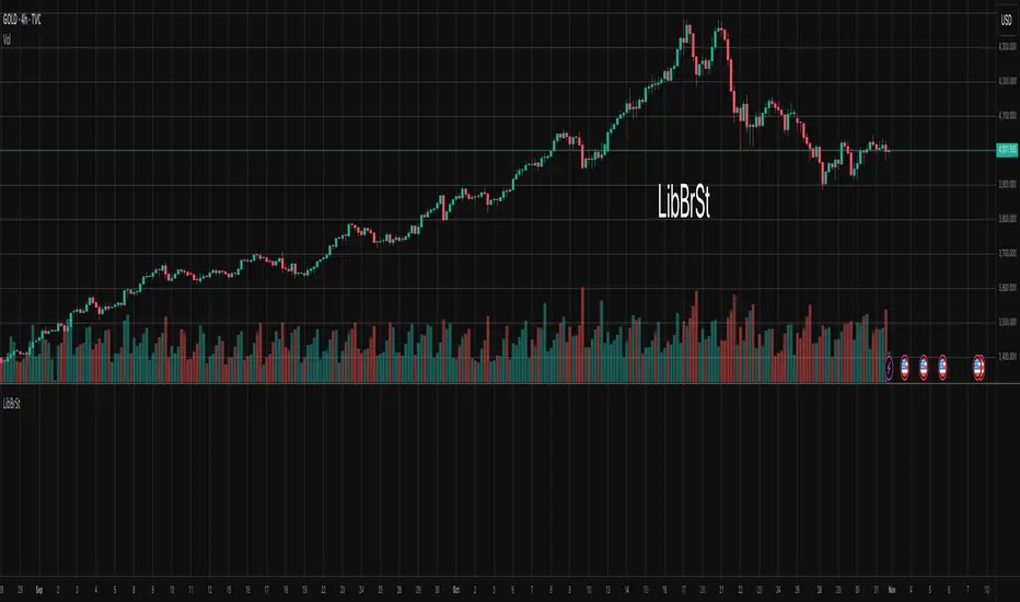
LibBrStLibrary "LibBrSt"
This is a library for quantitative analysis, designed to estimate
the statistical properties of price movements *within* a single
OHLC bar, without requiring access to tick data. It provides a
suite of estimators based on various statistical and econometric
models, allowing for analysis of intra-bar volatility and
price distribution.
Key Capabilities:
1. **Price Distribution Models (`PriceEst`):** Provides a selection
of estimators that model intra-bar price action as a probability
distribution over the range. This allows for the
calculation of the intra-bar mean (`priceMean`) and standard
deviation (`priceStdDev`) in absolute price units. Models include:
- **Symmetric Models:** `uniform`, `triangular`, `arcsine`,
`betaSym`, and `t4Sym` (Student-t with fat tails).
- **Skewed Models:** `betaSkew` and `t4Skew`, which adjust
their shape based on the Open/Close position.
- **Model Assumptions:** The skewed models rely on specific
internal constants. `betaSkew` uses a fixed concentration
parameter (`BETA_SKEW_CONCENTRATION = 4.0`), and `t4Sym`/`t4Skew`
use a heuristic scaling factor (`T4_SHAPE_FACTOR`)
to map the distribution.
2. **Econometric Log-Return Estimators (`LogEst`):** Includes a set of
econometric estimators for calculating the volatility (`logStdDev`)
and drift (`logMean`) of logarithmic returns within a single bar.
These are unit-less measures. Models include:
- **Parkinson (1980):** A High-Low range estimator.
- **Garman-Klass (1980):** An OHLC-based estimator.
- **Rogers-Satchell (1991):** An OHLC estimator that accounts
for non-zero drift.
3. **Distribution Analysis (PDF/CDF):** Provides functions to work
with the Probability Density Function (`pricePdf`) and
Cumulative Distribution Function (`priceCdf`) of the
chosen price model.
- **Note on `priceCdf`:** This function uses analytical (exact)
calculations for the `uniform`, `triangular`, and `arcsine`
models. For all other models (e.g., `betaSkew`, `t4Skew`),
it uses **numerical integration (Simpson's rule)** as
an approximation of the cumulative probability.
4. **Mathematical Functions:** The library's Beta distribution
models (`betaSym`, `betaSkew`) are supported by an internal
implementation of the natural log-gamma function, which is
based on the Lanczos approximation.
---
**DISCLAIMER**
This library is provided "AS IS" and for informational and
educational purposes only. It does not constitute financial,
investment, or trading advice.
The author assumes no liability for any errors, inaccuracies,
or omissions in the code. Using this library to build
trading indicators or strategies is entirely at your own risk.
As a developer using this library, you are solely responsible
for the rigorous testing, validation, and performance of any
scripts you create based on these functions. The author shall
not be held liable for any financial losses incurred directly
or indirectly from the use of this library or any scripts
derived from it.
priceStdDev(estimator, offset)
Estimates **σ̂** (standard deviation) *in price units* for the current
bar, according to the chosen `PriceEst` distribution assumption.
Parameters:
estimator (series PriceEst) : series PriceEst Distribution assumption (see enum).
offset (int) : series int To offset the calculated bar
Returns: series float σ̂ ≥ 0 ; `na` if undefined (e.g. zero range).
priceMean(estimator, offset)
Estimates **μ̂** (mean price) for the chosen `PriceEst` within the
current bar.
Parameters:
estimator (series PriceEst) : series PriceEst Distribution assumption (see enum).
offset (int) : series int To offset the calculated bar
Returns: series float μ̂ in price units.
pricePdf(estimator, price, offset)
Probability-density under the chosen `PriceEst` model.
**Returns 0** when `p` is outside the current bar’s .
Parameters:
estimator (series PriceEst) : series PriceEst Distribution assumption (see enum).
price (float) : series float Price level to evaluate.
offset (int) : series int To offset the calculated bar
Returns: series float Density value.
priceCdf(estimator, upper, lower, steps, offset)
Cumulative probability **between** `upper` and `lower` under
the chosen `PriceEst` model. Outside-bar regions contribute zero.
Uses a fast, analytical calculation for Uniform, Triangular, and
Arcsine distributions, and defaults to numerical integration
(Simpson's rule) for more complex models.
Parameters:
estimator (series PriceEst) : series PriceEst Distribution assumption (see enum).
upper (float) : series float Upper Integration Boundary.
lower (float) : series float Lower Integration Boundary.
steps (int) : series int # of sub-intervals for numerical integration (if used).
offset (int) : series int To offset the calculated bar.
Returns: series float Probability mass ∈ .
logStdDev(estimator, offset)
Estimates **σ̂** (standard deviation) of *log-returns* for the current bar.
Parameters:
estimator (series LogEst) : series LogEst Distribution assumption (see enum).
offset (int) : series int To offset the calculated bar
Returns: series float σ̂ (unit-less); `na` if undefined.
logMean(estimator, offset)
Estimates μ̂ (mean log-return / drift) for the chosen `LogEst`.
The returned value is consistent with the assumptions of the
selected volatility estimator.
Parameters:
estimator (series LogEst) : series LogEst Distribution assumption (see enum).
offset (int) : series int To offset the calculated bar
Returns: series float μ̂ (unit-less log-return).
LibWghtLibrary "LibWght"
This is a library of mathematical and statistical functions
designed for quantitative analysis in Pine Script. Its core
principle is the integration of a custom weighting series
(e.g., volume) into a wide array of standard technical
analysis calculations.
Key Capabilities:
1. **Universal Weighting:** All exported functions accept a `weight`
parameter. This allows standard calculations (like moving
averages, RSI, and standard deviation) to be influenced by an
external data series, such as volume or tick count.
2. **Weighted Averages and Indicators:** Includes a comprehensive
collection of weighted functions:
- **Moving Averages:** `wSma`, `wEma`, `wWma`, `wRma` (Wilder's),
`wHma` (Hull), and `wLSma` (Least Squares / Linear Regression).
- **Oscillators & Ranges:** `wRsi`, `wAtr` (Average True Range),
`wTr` (True Range), and `wR` (High-Low Range).
3. **Volatility Decomposition:** Provides functions to decompose
total variance into distinct components for market analysis.
- **Two-Way Decomposition (`wTotVar`):** Separates variance into
**between-bar** (directional) and **within-bar** (noise)
components.
- **Three-Way Decomposition (`wLRTotVar`):** Decomposes variance
relative to a linear regression into **Trend** (explained by
the LR slope), **Residual** (mean-reversion around the
LR line), and **Within-Bar** (noise) components.
- **Local Volatility (`wLRLocTotStdDev`):** Measures the total
"noise" (within-bar + residual) around the trend line.
4. **Weighted Statistics and Regression:** Provides a robust
function for Weighted Linear Regression (`wLinReg`) and a
full suite of related statistical measures:
- **Between-Bar Stats:** `wBtwVar`, `wBtwStdDev`, `wBtwStdErr`.
- **Residual Stats:** `wResVar`, `wResStdDev`, `wResStdErr`.
5. **Fallback Mechanism:** All functions are designed for reliability.
If the total weight over the lookback period is zero (e.g., in
a no-volume period), the algorithms automatically fall back to
their unweighted, uniform-weight equivalents (e.g., `wSma`
becomes a standard `ta.sma`), preventing errors and ensuring
continuous calculation.
---
**DISCLAIMER**
This library is provided "AS IS" and for informational and
educational purposes only. It does not constitute financial,
investment, or trading advice.
The author assumes no liability for any errors, inaccuracies,
or omissions in the code. Using this library to build
trading indicators or strategies is entirely at your own risk.
As a developer using this library, you are solely responsible
for the rigorous testing, validation, and performance of any
scripts you create based on these functions. The author shall
not be held liable for any financial losses incurred directly
or indirectly from the use of this library or any scripts
derived from it.
wSma(source, weight, length)
Weighted Simple Moving Average (linear kernel).
Parameters:
source (float) : series float Data to average.
weight (float) : series float Weight series.
length (int) : series int Look-back length ≥ 1.
Returns: series float Linear-kernel weighted mean; falls back to
the arithmetic mean if Σweight = 0.
wEma(source, weight, length)
Weighted EMA (exponential kernel).
Parameters:
source (float) : series float Data to average.
weight (float) : series float Weight series.
length (simple int) : simple int Look-back length ≥ 1.
Returns: series float Exponential-kernel weighted mean; falls
back to classic EMA if Σweight = 0.
wWma(source, weight, length)
Weighted WMA (linear kernel).
Parameters:
source (float) : series float Data to average.
weight (float) : series float Weight series.
length (int) : series int Look-back length ≥ 1.
Returns: series float Linear-kernel weighted mean; falls back to
classic WMA if Σweight = 0.
wRma(source, weight, length)
Weighted RMA (Wilder kernel, α = 1/len).
Parameters:
source (float) : series float Data to average.
weight (float) : series float Weight series.
length (simple int) : simple int Look-back length ≥ 1.
Returns: series float Wilder-kernel weighted mean; falls back to
classic RMA if Σweight = 0.
wHma(source, weight, length)
Weighted HMA (linear kernel).
Parameters:
source (float) : series float Data to average.
weight (float) : series float Weight series.
length (int) : series int Look-back length ≥ 1.
Returns: series float Linear-kernel weighted mean; falls back to
classic HMA if Σweight = 0.
wRsi(source, weight, length)
Weighted Relative Strength Index.
Parameters:
source (float) : series float Price series.
weight (float) : series float Weight series.
length (simple int) : simple int Look-back length ≥ 1.
Returns: series float Weighted RSI; uniform if Σw = 0.
wAtr(tr, weight, length)
Weighted ATR (Average True Range).
Implemented as WRMA on *true range*.
Parameters:
tr (float) : series float True Range series.
weight (float) : series float Weight series.
length (simple int) : simple int Look-back length ≥ 1.
Returns: series float Weighted ATR; uniform weights if Σw = 0.
wTr(tr, weight, length)
Weighted True Range over a window.
Parameters:
tr (float) : series float True Range series.
weight (float) : series float Weight series.
length (int) : series int Look-back length ≥ 1.
Returns: series float Weighted mean of TR; uniform if Σw = 0.
wR(r, weight, length)
Weighted High-Low Range over a window.
Parameters:
r (float) : series float High-Low per bar.
weight (float) : series float Weight series.
length (int) : series int Look-back length ≥ 1.
Returns: series float Weighted mean of range; uniform if Σw = 0.
wBtwVar(source, weight, length, biased)
Weighted Between Variance (biased/unbiased).
Parameters:
source (float) : series float Data series.
weight (float) : series float Weight series.
length (int) : series int Look-back length ≥ 2.
biased (bool) : series bool true → population (biased); false → sample.
Returns:
variance series float The calculated between-bar variance (σ²btw), either biased or unbiased.
sumW series float The sum of weights over the lookback period (Σw).
sumW2 series float The sum of squared weights over the lookback period (Σw²).
wBtwStdDev(source, weight, length, biased)
Weighted Between Standard Deviation.
Parameters:
source (float) : series float Data series.
weight (float) : series float Weight series.
length (int) : series int Look-back length ≥ 2.
biased (bool) : series bool true → population (biased); false → sample.
Returns: series float σbtw uniform if Σw = 0.
wBtwStdErr(source, weight, length, biased)
Weighted Between Standard Error.
Parameters:
source (float) : series float Data series.
weight (float) : series float Weight series.
length (int) : series int Look-back length ≥ 2.
biased (bool) : series bool true → population (biased); false → sample.
Returns: series float √(σ²btw / N_eff) uniform if Σw = 0.
wTotVar(mu, sigma, weight, length, biased)
Weighted Total Variance (= between-group + within-group).
Useful when each bar represents an aggregate with its own
mean* and pre-estimated σ (e.g., second-level ranges inside a
1-minute bar). Assumes the *weight* series applies to both the
group means and their σ estimates.
Parameters:
mu (float) : series float Group means (e.g., HL2 of 1-second bars).
sigma (float) : series float Pre-estimated σ of each group (same basis).
weight (float) : series float Weight series (volume, ticks, …).
length (int) : series int Look-back length ≥ 2.
biased (bool) : series bool true → population (biased); false → sample.
Returns:
varBtw series float The between-bar variance component (σ²btw).
varWtn series float The within-bar variance component (σ²wtn).
sumW series float The sum of weights over the lookback period (Σw).
sumW2 series float The sum of squared weights over the lookback period (Σw²).
wTotStdDev(mu, sigma, weight, length, biased)
Weighted Total Standard Deviation.
Parameters:
mu (float) : series float Group means (e.g., HL2 of 1-second bars).
sigma (float) : series float Pre-estimated σ of each group (same basis).
weight (float) : series float Weight series (volume, ticks, …).
length (int) : series int Look-back length ≥ 2.
biased (bool) : series bool true → population (biased); false → sample.
Returns: series float σtot.
wTotStdErr(mu, sigma, weight, length, biased)
Weighted Total Standard Error.
SE = √( total variance / N_eff ) with the same effective sample
size logic as `wster()`.
Parameters:
mu (float) : series float Group means (e.g., HL2 of 1-second bars).
sigma (float) : series float Pre-estimated σ of each group (same basis).
weight (float) : series float Weight series (volume, ticks, …).
length (int) : series int Look-back length ≥ 2.
biased (bool) : series bool true → population (biased); false → sample.
Returns: series float √(σ²tot / N_eff).
wLinReg(source, weight, length)
Weighted Linear Regression.
Parameters:
source (float) : series float Data series.
weight (float) : series float Weight series.
length (int) : series int Look-back length ≥ 2.
Returns:
mid series float The estimated value of the regression line at the most recent bar.
slope series float The slope of the regression line.
intercept series float The intercept of the regression line.
wResVar(source, weight, midLine, slope, length, biased)
Weighted Residual Variance.
linear regression – optionally biased (population) or
unbiased (sample).
Parameters:
source (float) : series float Data series.
weight (float) : series float Weighting series (volume, etc.).
midLine (float) : series float Regression value at the last bar.
slope (float) : series float Slope per bar.
length (int) : series int Look-back length ≥ 2.
biased (bool) : series bool true → population variance (σ²_P), denominator ≈ N_eff.
false → sample variance (σ²_S), denominator ≈ N_eff - 2.
(Adjusts for 2 degrees of freedom lost to the regression).
Returns:
variance series float The calculated residual variance (σ²res), either biased or unbiased.
sumW series float The sum of weights over the lookback period (Σw).
sumW2 series float The sum of squared weights over the lookback period (Σw²).
wResStdDev(source, weight, midLine, slope, length, biased)
Weighted Residual Standard Deviation.
Parameters:
source (float) : series float Data series.
weight (float) : series float Weight series.
midLine (float) : series float Regression value at the last bar.
slope (float) : series float Slope per bar.
length (int) : series int Look-back length ≥ 2.
biased (bool) : series bool true → population (biased); false → sample.
Returns: series float σres; uniform if Σw = 0.
wResStdErr(source, weight, midLine, slope, length, biased)
Weighted Residual Standard Error.
Parameters:
source (float) : series float Data series.
weight (float) : series float Weight series.
midLine (float) : series float Regression value at the last bar.
slope (float) : series float Slope per bar.
length (int) : series int Look-back length ≥ 2.
biased (bool) : series bool true → population (biased); false → sample.
Returns: series float √(σ²res / N_eff); uniform if Σw = 0.
wLRTotVar(mu, sigma, weight, midLine, slope, length, biased)
Weighted Linear-Regression Total Variance **around the
window’s weighted mean μ**.
σ²_tot = E_w ⟶ *within-group variance*
+ Var_w ⟶ *residual variance*
+ Var_w ⟶ *trend variance*
where each bar i in the look-back window contributes
m_i = *mean* (e.g. 1-sec HL2)
σ_i = *sigma* (pre-estimated intrabar σ)
w_i = *weight* (volume, ticks, …)
ŷ_i = b₀ + b₁·x (value of the weighted LR line)
r_i = m_i − ŷ_i (orthogonal residual)
Parameters:
mu (float) : series float Per-bar mean m_i.
sigma (float) : series float Pre-estimated σ_i of each bar.
weight (float) : series float Weight series w_i (≥ 0).
midLine (float) : series float Regression value at the latest bar (ŷₙ₋₁).
slope (float) : series float Slope b₁ of the regression line.
length (int) : series int Look-back length ≥ 2.
biased (bool) : series bool true → population; false → sample.
Returns:
varRes series float The residual variance component (σ²res).
varWtn series float The within-bar variance component (σ²wtn).
varTrd series float The trend variance component (σ²trd), explained by the linear regression.
sumW series float The sum of weights over the lookback period (Σw).
sumW2 series float The sum of squared weights over the lookback period (Σw²).
wLRTotStdDev(mu, sigma, weight, midLine, slope, length, biased)
Weighted Linear-Regression Total Standard Deviation.
Parameters:
mu (float) : series float Per-bar mean m_i.
sigma (float) : series float Pre-estimated σ_i of each bar.
weight (float) : series float Weight series w_i (≥ 0).
midLine (float) : series float Regression value at the latest bar (ŷₙ₋₁).
slope (float) : series float Slope b₁ of the regression line.
length (int) : series int Look-back length ≥ 2.
biased (bool) : series bool true → population; false → sample.
Returns: series float √(σ²tot).
wLRTotStdErr(mu, sigma, weight, midLine, slope, length, biased)
Weighted Linear-Regression Total Standard Error.
SE = √( σ²_tot / N_eff ) with N_eff = Σw² / Σw² (like in wster()).
Parameters:
mu (float) : series float Per-bar mean m_i.
sigma (float) : series float Pre-estimated σ_i of each bar.
weight (float) : series float Weight series w_i (≥ 0).
midLine (float) : series float Regression value at the latest bar (ŷₙ₋₁).
slope (float) : series float Slope b₁ of the regression line.
length (int) : series int Look-back length ≥ 2.
biased (bool) : series bool true → population; false → sample.
Returns: series float √((σ²res, σ²wtn, σ²trd) / N_eff).
wLRLocTotStdDev(mu, sigma, weight, midLine, slope, length, biased)
Weighted Linear-Regression Local Total Standard Deviation.
Measures the total "noise" (within-bar + residual) around the trend.
Parameters:
mu (float) : series float Per-bar mean m_i.
sigma (float) : series float Pre-estimated σ_i of each bar.
weight (float) : series float Weight series w_i (≥ 0).
midLine (float) : series float Regression value at the latest bar (ŷₙ₋₁).
slope (float) : series float Slope b₁ of the regression line.
length (int) : series int Look-back length ≥ 2.
biased (bool) : series bool true → population; false → sample.
Returns: series float √(σ²wtn + σ²res).
wLRLocTotStdErr(mu, sigma, weight, midLine, slope, length, biased)
Weighted Linear-Regression Local Total Standard Error.
Parameters:
mu (float) : series float Per-bar mean m_i.
sigma (float) : series float Pre-estimated σ_i of each bar.
weight (float) : series float Weight series w_i (≥ 0).
midLine (float) : series float Regression value at the latest bar (ŷₙ₋₁).
slope (float) : series float Slope b₁ of the regression line.
length (int) : series int Look-back length ≥ 2.
biased (bool) : series bool true → population; false → sample.
Returns: series float √((σ²wtn + σ²res) / N_eff).
wLSma(source, weight, length)
Weighted Least Square Moving Average.
Parameters:
source (float) : series float Data series.
weight (float) : series float Weight series.
length (int) : series int Look-back length ≥ 2.
Returns: series float Least square weighted mean. Falls back
to unweighted regression if Σw = 0.
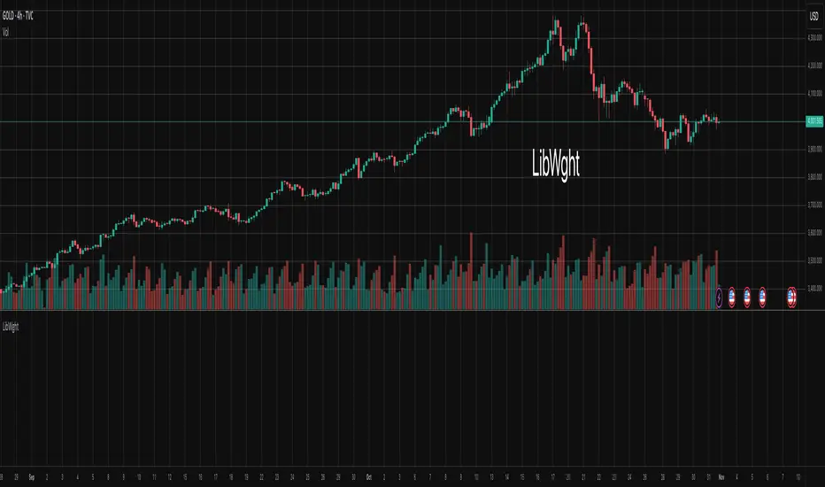
LogNormalLibrary "LogNormal"
A collection of functions used to model skewed distributions as log-normal.
Prices are commonly modeled using log-normal distributions (ie. Black-Scholes) because they exhibit multiplicative changes with long tails; skewed exponential growth and high variance. This approach is particularly useful for understanding price behavior and estimating risk, assuming continuously compounding returns are normally distributed.
Because log space analysis is not as direct as using math.log(price) , this library extends the Error Functions library to make working with log-normally distributed data as simple as possible.
- - -
QUICK START
Import library into your project
Initialize model with a mean and standard deviation
Pass model params between methods to compute various properties
var LogNorm model = LN.init(arr.avg(), arr.stdev()) // Assumes the library is imported as LN
var mode = model.mode()
Outputs from the model can be adjusted to better fit the data.
var Quantile data = arr.quantiles()
var more_accurate_mode = mode.fit(model, data) // Fits value from model to data
Inputs to the model can also be adjusted to better fit the data.
datum = 123.45
model_equivalent_datum = datum.fit(data, model) // Fits value from data to the model
area_from_zero_to_datum = model.cdf(model_equivalent_datum)
- - -
TYPES
There are two requisite UDTs: LogNorm and Quantile . They are used to pass parameters between functions and are set automatically (see Type Management ).
LogNorm
Object for log space parameters and linear space quantiles .
Fields:
mu (float) : Log space mu ( µ ).
sigma (float) : Log space sigma ( σ ).
variance (float) : Log space variance ( σ² ).
quantiles (Quantile) : Linear space quantiles.
Quantile
Object for linear quantiles, most similar to a seven-number summary .
Fields:
Q0 (float) : Smallest Value
LW (float) : Lower Whisker Endpoint
LC (float) : Lower Whisker Crosshatch
Q1 (float) : First Quartile
Q2 (float) : Second Quartile
Q3 (float) : Third Quartile
UC (float) : Upper Whisker Crosshatch
UW (float) : Upper Whisker Endpoint
Q4 (float) : Largest Value
IQR (float) : Interquartile Range
MH (float) : Midhinge
TM (float) : Trimean
MR (float) : Mid-Range
- - -
TYPE MANAGEMENT
These functions reliably initialize and update the UDTs. Because parameterization is interdependent, avoid setting the LogNorm and Quantile fields directly .
init(mean, stdev, variance)
Initializes a LogNorm object.
Parameters:
mean (float) : Linearly measured mean.
stdev (float) : Linearly measured standard deviation.
variance (float) : Linearly measured variance.
Returns: LogNorm Object
set(ln, mean, stdev, variance)
Transforms linear measurements into log space parameters for a LogNorm object.
Parameters:
ln (LogNorm) : Object containing log space parameters.
mean (float) : Linearly measured mean.
stdev (float) : Linearly measured standard deviation.
variance (float) : Linearly measured variance.
Returns: LogNorm Object
quantiles(arr)
Gets empirical quantiles from an array of floats.
Parameters:
arr (array) : Float array object.
Returns: Quantile Object
- - -
DESCRIPTIVE STATISTICS
Using only the initialized LogNorm parameters, these functions compute a model's central tendency and standardized moments.
mean(ln)
Computes the linear mean from log space parameters.
Parameters:
ln (LogNorm) : Object containing log space parameters.
Returns: Between 0 and ∞
median(ln)
Computes the linear median from log space parameters.
Parameters:
ln (LogNorm) : Object containing log space parameters.
Returns: Between 0 and ∞
mode(ln)
Computes the linear mode from log space parameters.
Parameters:
ln (LogNorm) : Object containing log space parameters.
Returns: Between 0 and ∞
variance(ln)
Computes the linear variance from log space parameters.
Parameters:
ln (LogNorm) : Object containing log space parameters.
Returns: Between 0 and ∞
skewness(ln)
Computes the linear skewness from log space parameters.
Parameters:
ln (LogNorm) : Object containing log space parameters.
Returns: Between 0 and ∞
kurtosis(ln, excess)
Computes the linear kurtosis from log space parameters.
Parameters:
ln (LogNorm) : Object containing log space parameters.
excess (bool) : Excess Kurtosis (true) or regular Kurtosis (false).
Returns: Between 0 and ∞
hyper_skewness(ln)
Computes the linear hyper skewness from log space parameters.
Parameters:
ln (LogNorm) : Object containing log space parameters.
Returns: Between 0 and ∞
hyper_kurtosis(ln, excess)
Computes the linear hyper kurtosis from log space parameters.
Parameters:
ln (LogNorm) : Object containing log space parameters.
excess (bool) : Excess Hyper Kurtosis (true) or regular Hyper Kurtosis (false).
Returns: Between 0 and ∞
- - -
DISTRIBUTION FUNCTIONS
These wrap Gaussian functions to make working with model space more direct. Because they are contained within a log-normal library, they describe estimations relative to a log-normal curve, even though they fundamentally measure a Gaussian curve.
pdf(ln, x, empirical_quantiles)
A Probability Density Function estimates the probability density . For clarity, density is not a probability .
Parameters:
ln (LogNorm) : Object of log space parameters.
x (float) : Linear X coordinate for which a density will be estimated.
empirical_quantiles (Quantile) : Quantiles as observed in the data (optional).
Returns: Between 0 and ∞
cdf(ln, x, precise)
A Cumulative Distribution Function estimates the area under a Log-Normal curve between Zero and a linear X coordinate.
Parameters:
ln (LogNorm) : Object of log space parameters.
x (float) : Linear X coordinate .
precise (bool) : Double precision (true) or single precision (false).
Returns: Between 0 and 1
ccdf(ln, x, precise)
A Complementary Cumulative Distribution Function estimates the area under a Log-Normal curve between a linear X coordinate and Infinity.
Parameters:
ln (LogNorm) : Object of log space parameters.
x (float) : Linear X coordinate .
precise (bool) : Double precision (true) or single precision (false).
Returns: Between 0 and 1
cdfinv(ln, a, precise)
An Inverse Cumulative Distribution Function reverses the Log-Normal cdf() by estimating the linear X coordinate from an area.
Parameters:
ln (LogNorm) : Object of log space parameters.
a (float) : Normalized area .
precise (bool) : Double precision (true) or single precision (false).
Returns: Between 0 and ∞
ccdfinv(ln, a, precise)
An Inverse Complementary Cumulative Distribution Function reverses the Log-Normal ccdf() by estimating the linear X coordinate from an area.
Parameters:
ln (LogNorm) : Object of log space parameters.
a (float) : Normalized area .
precise (bool) : Double precision (true) or single precision (false).
Returns: Between 0 and ∞
cdfab(ln, x1, x2, precise)
A Cumulative Distribution Function from A to B estimates the area under a Log-Normal curve between two linear X coordinates (A and B).
Parameters:
ln (LogNorm) : Object of log space parameters.
x1 (float) : First linear X coordinate .
x2 (float) : Second linear X coordinate .
precise (bool) : Double precision (true) or single precision (false).
Returns: Between 0 and 1
ott(ln, x, precise)
A One-Tailed Test transforms a linear X coordinate into an absolute Z Score before estimating the area under a Log-Normal curve between Z and Infinity.
Parameters:
ln (LogNorm) : Object of log space parameters.
x (float) : Linear X coordinate .
precise (bool) : Double precision (true) or single precision (false).
Returns: Between 0 and 0.5
ttt(ln, x, precise)
A Two-Tailed Test transforms a linear X coordinate into symmetrical ± Z Scores before estimating the area under a Log-Normal curve from Zero to -Z, and +Z to Infinity.
Parameters:
ln (LogNorm) : Object of log space parameters.
x (float) : Linear X coordinate .
precise (bool) : Double precision (true) or single precision (false).
Returns: Between 0 and 1
ottinv(ln, a, precise)
An Inverse One-Tailed Test reverses the Log-Normal ott() by estimating a linear X coordinate for the right tail from an area.
Parameters:
ln (LogNorm) : Object of log space parameters.
a (float) : Half a normalized area .
precise (bool) : Double precision (true) or single precision (false).
Returns: Between 0 and ∞
tttinv(ln, a, precise)
An Inverse Two-Tailed Test reverses the Log-Normal ttt() by estimating two linear X coordinates from an area.
Parameters:
ln (LogNorm) : Object of log space parameters.
a (float) : Normalized area .
precise (bool) : Double precision (true) or single precision (false).
Returns: Linear space tuple :
- - -
UNCERTAINTY
Model-based measures of uncertainty, information, and risk.
sterr(sample_size, fisher_info)
The standard error of a sample statistic.
Parameters:
sample_size (float) : Number of observations.
fisher_info (float) : Fisher information.
Returns: Between 0 and ∞
surprisal(p, base)
Quantifies the information content of a single event.
Parameters:
p (float) : Probability of the event .
base (float) : Logarithmic base (optional).
Returns: Between 0 and ∞
entropy(ln, base)
Computes the differential entropy (average surprisal).
Parameters:
ln (LogNorm) : Object of log space parameters.
base (float) : Logarithmic base (optional).
Returns: Between 0 and ∞
perplexity(ln, base)
Computes the average number of distinguishable outcomes from the entropy.
Parameters:
ln (LogNorm)
base (float) : Logarithmic base used for Entropy (optional).
Returns: Between 0 and ∞
value_at_risk(ln, p, precise)
Estimates a risk threshold under normal market conditions for a given confidence level.
Parameters:
ln (LogNorm) : Object of log space parameters.
p (float) : Probability threshold, aka. the confidence level .
precise (bool) : Double precision (true) or single precision (false).
Returns: Between 0 and ∞
value_at_risk_inv(ln, value_at_risk, precise)
Reverses the value_at_risk() by estimating the confidence level from the risk threshold.
Parameters:
ln (LogNorm) : Object of log space parameters.
value_at_risk (float) : Value at Risk.
precise (bool) : Double precision (true) or single precision (false).
Returns: Between 0 and 1
conditional_value_at_risk(ln, p, precise)
Estimates the average loss beyond a confidence level, aka. expected shortfall.
Parameters:
ln (LogNorm) : Object of log space parameters.
p (float) : Probability threshold, aka. the confidence level .
precise (bool) : Double precision (true) or single precision (false).
Returns: Between 0 and ∞
conditional_value_at_risk_inv(ln, conditional_value_at_risk, precise)
Reverses the conditional_value_at_risk() by estimating the confidence level of an average loss.
Parameters:
ln (LogNorm) : Object of log space parameters.
conditional_value_at_risk (float) : Conditional Value at Risk.
precise (bool) : Double precision (true) or single precision (false).
Returns: Between 0 and 1
partial_expectation(ln, x, precise)
Estimates the partial expectation of a linear X coordinate.
Parameters:
ln (LogNorm) : Object of log space parameters.
x (float) : Linear X coordinate .
precise (bool) : Double precision (true) or single precision (false).
Returns: Between 0 and µ
partial_expectation_inv(ln, partial_expectation, precise)
Reverses the partial_expectation() by estimating a linear X coordinate.
Parameters:
ln (LogNorm) : Object of log space parameters.
partial_expectation (float) : Partial Expectation .
precise (bool) : Double precision (true) or single precision (false).
Returns: Between 0 and ∞
conditional_expectation(ln, x, precise)
Estimates the conditional expectation of a linear X coordinate.
Parameters:
ln (LogNorm) : Object of log space parameters.
x (float) : Linear X coordinate .
precise (bool) : Double precision (true) or single precision (false).
Returns: Between X and ∞
conditional_expectation_inv(ln, conditional_expectation, precise)
Reverses the conditional_expectation by estimating a linear X coordinate.
Parameters:
ln (LogNorm) : Object of log space parameters.
conditional_expectation (float) : Conditional Expectation .
precise (bool) : Double precision (true) or single precision (false).
Returns: Between 0 and ∞
fisher(ln, log)
Computes the Fisher Information Matrix for the distribution, not a linear X coordinate.
Parameters:
ln (LogNorm) : Object of log space parameters.
log (bool) : Sets if the matrix should be in log (true) or linear (false) space.
Returns: FIM for the distribution
fisher(ln, x, log)
Computes the Fisher Information Matrix for a linear X coordinate, not the distribution itself.
Parameters:
ln (LogNorm) : Object of log space parameters.
x (float) : Linear X coordinate .
log (bool) : Sets if the matrix should be in log (true) or linear (false) space.
Returns: FIM for the linear X coordinate
confidence_interval(ln, x, sample_size, confidence, precise)
Estimates a confidence interval for a linear X coordinate.
Parameters:
ln (LogNorm) : Object of log space parameters.
x (float) : Linear X coordinate .
sample_size (float) : Number of observations.
confidence (float) : Confidence level .
precise (bool) : Double precision (true) or single precision (false).
Returns: CI for the linear X coordinate
- - -
CURVE FITTING
An overloaded function that helps transform values between spaces. The primary function uses quantiles, and the overloads wrap the primary function to make working with LogNorm more direct.
fit(x, a, b)
Transforms X coordinate between spaces A and B.
Parameters:
x (float) : Linear X coordinate from space A .
a (LogNorm | Quantile | array) : LogNorm, Quantile, or float array.
b (LogNorm | Quantile | array) : LogNorm, Quantile, or float array.
Returns: Adjusted X coordinate
- - -
EXPORTED HELPERS
Small utilities to simplify extensibility.
z_score(ln, x)
Converts a linear X coordinate into a Z Score.
Parameters:
ln (LogNorm) : Object of log space parameters.
x (float) : Linear X coordinate.
Returns: Between -∞ and +∞
x_coord(ln, z)
Converts a Z Score into a linear X coordinate.
Parameters:
ln (LogNorm) : Object of log space parameters.
z (float) : Standard normal Z Score.
Returns: Between 0 and ∞
iget(arr, index)
Gets an interpolated value of a pseudo -element (fictional element between real array elements). Useful for quantile mapping.
Parameters:
arr (array) : Float array object.
index (float) : Index of the pseudo element.
Returns: Interpolated value of the arrays pseudo element.

ICOptimizerLibrary "ICOptimizer"
Library for IC-based parameter optimization
findOptimalParam(testParams, icValues, currentParam, smoothing)
Find optimal parameter from array of IC values
Parameters:
testParams (array) : Array of parameter values being tested
icValues (array) : Array of IC values for each parameter (same size as testParams)
currentParam (float) : Current parameter value (for smoothing)
smoothing (simple float) : Smoothing factor (0-1, e.g., 0.2 means 20% new, 80% old)
Returns: New parameter value, its IC, and array index
adaptiveParamWithStarvation(opt, testParams, icValues, smoothing, starvationThreshold, starvationJumpSize)
Adaptive parameter selection with starvation handling
Parameters:
opt (ICOptimizer) : ICOptimizer object
testParams (array) : Array of parameter values
icValues (array) : Array of IC values for each parameter
smoothing (simple float) : Normal smoothing factor
starvationThreshold (simple int) : Number of updates before triggering starvation mode
starvationJumpSize (simple float) : Jump size when in starvation (as fraction of range)
Returns: Updated parameter and IC
detectAndAdjustDomination(longCount, shortCount, currentLongLevel, currentShortLevel, dominationRatio, jumpSize, minLevel, maxLevel)
Detect signal imbalance and adjust parameters
Parameters:
longCount (int) : Number of long signals in period
shortCount (int) : Number of short signals in period
currentLongLevel (float) : Current long threshold
currentShortLevel (float) : Current short threshold
dominationRatio (simple int) : Ratio threshold (e.g., 4 = 4:1 imbalance)
jumpSize (simple float) : Size of adjustment
minLevel (simple float) : Minimum allowed level
maxLevel (simple float) : Maximum allowed level
Returns:
calcIC(signals, returns, lookback)
Parameters:
signals (float)
returns (float)
lookback (simple int)
classifyIC(currentIC, icWindow, goodPercentile, badPercentile)
Parameters:
currentIC (float)
icWindow (simple int)
goodPercentile (simple int)
badPercentile (simple int)
evaluateSignal(signal, forwardReturn)
Parameters:
signal (float)
forwardReturn (float)
updateOptimizerState(opt, signal, forwardReturn, currentIC, metaICPeriod)
Parameters:
opt (ICOptimizer)
signal (float)
forwardReturn (float)
currentIC (float)
metaICPeriod (simple int)
calcSuccessRate(successful, total)
Parameters:
successful (int)
total (int)
createICStatsTable(opt, paramName, normalSuccess, normalTotal)
Parameters:
opt (ICOptimizer)
paramName (string)
normalSuccess (int)
normalTotal (int)
initOptimizer(initialParam)
Parameters:
initialParam (float)
ICOptimizer
Fields:
currentParam (series float)
currentIC (series float)
metaIC (series float)
totalSignals (series int)
successfulSignals (series int)
goodICSignals (series int)
goodICSuccess (series int)
nonBadICSignals (series int)
nonBadICSuccess (series int)
goodICThreshold (series float)
badICThreshold (series float)
updateCounter (series int)

IC optimiser libLibrary "IC optimiser lib"
Library for IC-based parameter optimization
findOptimalParam(testParams, icValues, currentParam, smoothing)
Find optimal parameter from array of IC values
Parameters:
testParams (array) : Array of parameter values being tested
icValues (array) : Array of IC values for each parameter (same size as testParams)
currentParam (float) : Current parameter value (for smoothing)
smoothing (simple float) : Smoothing factor (0-1, e.g., 0.2 means 20% new, 80% old)
Returns: New parameter value, its IC, and array index
adaptiveParamWithStarvation(opt, testParams, icValues, smoothing, starvationThreshold, starvationJumpSize)
Adaptive parameter selection with starvation handling
Parameters:
opt (ICOptimizer) : ICOptimizer object
testParams (array) : Array of parameter values
icValues (array) : Array of IC values for each parameter
smoothing (simple float) : Normal smoothing factor
starvationThreshold (simple int) : Number of updates before triggering starvation mode
starvationJumpSize (simple float) : Jump size when in starvation (as fraction of range)
Returns: Updated parameter and IC
detectAndAdjustDomination(longCount, shortCount, currentLongLevel, currentShortLevel, dominationRatio, jumpSize, minLevel, maxLevel)
Detect signal imbalance and adjust parameters
Parameters:
longCount (int) : Number of long signals in period
shortCount (int) : Number of short signals in period
currentLongLevel (float) : Current long threshold
currentShortLevel (float) : Current short threshold
dominationRatio (simple int) : Ratio threshold (e.g., 4 = 4:1 imbalance)
jumpSize (simple float) : Size of adjustment
minLevel (simple float) : Minimum allowed level
maxLevel (simple float) : Maximum allowed level
Returns:
calcIC(signals, returns, lookback)
Parameters:
signals (float)
returns (float)
lookback (simple int)
classifyIC(currentIC, icWindow, goodPercentile, badPercentile)
Parameters:
currentIC (float)
icWindow (simple int)
goodPercentile (simple int)
badPercentile (simple int)
evaluateSignal(signal, forwardReturn)
Parameters:
signal (float)
forwardReturn (float)
updateOptimizerState(opt, signal, forwardReturn, currentIC, metaICPeriod)
Parameters:
opt (ICOptimizer)
signal (float)
forwardReturn (float)
currentIC (float)
metaICPeriod (simple int)
calcSuccessRate(successful, total)
Parameters:
successful (int)
total (int)
createICStatsTable(opt, paramName, normalSuccess, normalTotal)
Parameters:
opt (ICOptimizer)
paramName (string)
normalSuccess (int)
normalTotal (int)
initOptimizer(initialParam)
Parameters:
initialParam (float)
ICOptimizer
Fields:
currentParam (series float)
currentIC (series float)
metaIC (series float)
totalSignals (series int)
successfulSignals (series int)
goodICSignals (series int)
goodICSuccess (series int)
nonBadICSignals (series int)
nonBadICSuccess (series int)
goodICThreshold (series float)
badICThreshold (series float)
updateCounter (series int)

UTBotLibrary "UTBot"
is a powerful and flexible trading toolkit implemented in Pine Script. Based on the widely recognized UT Bot strategy originally developed by Yo_adriiiiaan with important enhancements by HPotter, this library provides users with customizable functions for dynamic trailing stop calculations using ATR (Average True Range), trend detection, and signal generation. It enables developers and traders to seamlessly integrate UT Bot logic into their own indicators and strategies without duplicating code.
Key features include:
Accurate ATR-based trailing stop and reversal detection
Multi-timeframe support for enhanced signal reliability
Clean and efficient API for easy integration and customization
Detailed documentation and examples for quick adoption
Open-source and community-friendly, encouraging collaboration and improvements
We sincerely thank Yo_adriiiiaan for the original UT Bot concept and HPotter for valuable improvements that have made this strategy even more robust. This library aims to honor their work by making the UT Bot methodology accessible to Pine Script developers worldwide.
This library is designed for Pine Script programmers looking to leverage the proven UT Bot methodology to build robust trading systems with minimal effort and maximum maintainability.
UTBot(h, l, c, multi, leng)
Parameters:
h (float) - high
l (float) - low
c (float)-close
multi (float)- multi for ATR
leng (int)-length for ATR
Returns:
xATRTS - ATR Based TrailingStop Value
pos - pos==1, long position, pos==-1, shot position
signal - 0 no signal, 1 buy, -1 sell

JK_Traders_Reality_LibLibrary "JK_Traders_Reality_Lib"
This library contains common elements used in Traders Reality scripts
calcPvsra(pvsraVolume, pvsraHigh, pvsraLow, pvsraClose, pvsraOpen, redVectorColor, greenVectorColor, violetVectorColor, blueVectorColor, darkGreyCandleColor, lightGrayCandleColor)
calculate the pvsra candle color and return the color as well as an alert if a vector candle has apperared.
Situation "Climax"
Bars with volume >= 200% of the average volume of the 10 previous chart TFs, or bars
where the product of candle spread x candle volume is >= the highest for the 10 previous
chart time TFs.
Default Colors: Bull bars are green and bear bars are red.
Situation "Volume Rising Above Average"
Bars with volume >= 150% of the average volume of the 10 previous chart TFs.
Default Colors: Bull bars are blue and bear are violet.
Parameters:
pvsraVolume (float) : the instrument volume series (obtained from request.sequrity)
pvsraHigh (float) : the instrument high series (obtained from request.sequrity)
pvsraLow (float) : the instrument low series (obtained from request.sequrity)
pvsraClose (float) : the instrument close series (obtained from request.sequrity)
pvsraOpen (float) : the instrument open series (obtained from request.sequrity)
redVectorColor (simple color) : red vector candle color
greenVectorColor (simple color) : green vector candle color
violetVectorColor (simple color) : violet/pink vector candle color
blueVectorColor (simple color) : blue vector candle color
darkGreyCandleColor (simple color) : regular volume candle down candle color - not a vector
lightGrayCandleColor (simple color) : regular volume candle up candle color - not a vector
@return
adr(length, barsBack)
Parameters:
length (simple int) : how many elements of the series to calculate on
barsBack (simple int) : starting possition for the length calculation - current bar or some other value eg last bar
@return adr the adr for the specified lenght
adrHigh(adr, fromDo)
Calculate the ADR high given an ADR
Parameters:
adr (float) : the adr
fromDo (simple bool) : boolean flag, if false calculate traditional adr from high low of today, if true calcualte from exchange midnight
@return adrHigh the position of the adr high in price
adrLow(adr, fromDo)
Parameters:
adr (float) : the adr
fromDo (simple bool) : boolean flag, if false calculate traditional adr from high low of today, if true calcualte from exchange midnight
@return adrLow the position of the adr low in price
splitSessionString(sessXTime)
given a session in the format 0000-0100:23456 split out the hours and minutes
Parameters:
sessXTime (simple string) : the session time string usually in the format 0000-0100:23456
@return
calcSessionStartEnd(sessXTime, gmt)
calculate the start and end timestamps of the session
Parameters:
sessXTime (simple string) : the session time string usually in the format 0000-0100:23456
gmt (simple string) : the gmt offset string usually in the format GMT+1 or GMT+2 etc
@return
drawOpenRange(sessXTime, sessXcol, showOrX, gmt)
draw open range for a session
Parameters:
sessXTime (simple string) : session string in the format 0000-0100:23456
sessXcol (simple color) : the color to be used for the opening range box shading
showOrX (simple bool) : boolean flag to toggle displaying the opening range
gmt (simple string) : the gmt offset string usually in the format GMT+1 or GMT+2 etc
@return void
drawSessionHiLo(sessXTime, showRectangleX, showLabelX, sessXcolLabel, sessXLabel, gmt, sessionLineStyle)
Parameters:
sessXTime (simple string) : session string in the format 0000-0100:23456
showRectangleX (simple bool)
showLabelX (simple bool)
sessXcolLabel (simple color) : the color to be used for the hi/low lines and label
sessXLabel (simple string) : the session label text
gmt (simple string) : the gmt offset string usually in the format GMT+1 or GMT+2 etc
sessionLineStyle (simple string) : the line stile for the session high low lines
@return void
calcDst()
calculate market session dst on/off flags
@return indicating if DST is on or off for a particular region
timestampPreviousDayOfWeek(previousDayOfWeek, hourOfDay, gmtOffset, oneWeekMillis)
Timestamp any of the 6 previous days in the week (such as last Wednesday at 21 hours GMT)
Parameters:
previousDayOfWeek (simple string) : Monday or Satruday
hourOfDay (simple int) : the hour of the day when psy calc is to start
gmtOffset (simple string) : the gmt offset string usually in the format GMT+1 or GMT+2 etc
oneWeekMillis (simple int) : the amount if time for a week in milliseconds
@return the timestamp of the psy level calculation start time
getdayOpen()
get the daily open - basically exchange midnight
@return the daily open value which is float price
newBar(res)
new_bar: check if we're on a new bar within the session in a given resolution
Parameters:
res (simple string) : the desired resolution
@return true/false is a new bar for the session has started
toPips(val)
to_pips Convert value to pips
Parameters:
val (float) : the value to convert to pips
@return the value in pips
rLabel(ry, rtext, rstyle, rcolor, valid, labelXOffset)
a function that draws a right aligned lable for a series during the current bar
Parameters:
ry (float) : series float the y coordinate of the lable
rtext (simple string) : the text of the label
rstyle (simple string) : the style for the lable
rcolor (simple color) : the color for the label
valid (simple bool) : a boolean flag that allows for turning on or off a lable
labelXOffset (int) : how much to offset the label from the current position
rLabelOffset(ry, rtext, rstyle, rcolor, valid, labelOffset)
a function that draws a right aligned lable for a series during the current bar
Parameters:
ry (float) : series float the y coordinate of the lable
rtext (string) : the text of the label
rstyle (simple string) : the style for the lable
rcolor (simple color) : the color for the label
valid (simple bool) : a boolean flag that allows for turning on or off a lable
labelOffset (int)
rLabelLastBar(ry, rtext, rstyle, rcolor, valid, labelXOffset)
a function that draws a right aligned lable for a series only on the last bar
Parameters:
ry (float) : series float the y coordinate of the lable
rtext (string) : the text of the label
rstyle (simple string) : the style for the lable
rcolor (simple color) : the color for the label
valid (simple bool) : a boolean flag that allows for turning on or off a lable
labelXOffset (int) : how much to offset the label from the current position
drawLine(xSeries, res, tag, xColor, xStyle, xWidth, xExtend, isLabelValid, xLabelOffset, validTimeFrame)
a function that draws a line and a label for a series
Parameters:
xSeries (float) : series float the y coordinate of the line/label
res (simple string) : the desired resolution controlling when a new line will start
tag (simple string) : the text for the lable
xColor (simple color) : the color for the label
xStyle (simple string) : the style for the line
xWidth (simple int) : the width of the line
xExtend (simple string) : extend the line
isLabelValid (simple bool) : a boolean flag that allows for turning on or off a label
xLabelOffset (int)
validTimeFrame (simple bool) : a boolean flag that allows for turning on or off a line drawn
drawLineDO(xSeries, res, tag, xColor, xStyle, xWidth, xExtend, isLabelValid, xLabelOffset, validTimeFrame)
a function that draws a line and a label for the daily open series
Parameters:
xSeries (float) : series float the y coordinate of the line/label
res (simple string) : the desired resolution controlling when a new line will start
tag (simple string) : the text for the lable
xColor (simple color) : the color for the label
xStyle (simple string) : the style for the line
xWidth (simple int) : the width of the line
xExtend (simple string) : extend the line
isLabelValid (simple bool) : a boolean flag that allows for turning on or off a label
xLabelOffset (int)
validTimeFrame (simple bool) : a boolean flag that allows for turning on or off a line drawn
drawPivot(pivotLevel, res, tag, pivotColor, pivotLabelColor, pivotStyle, pivotWidth, pivotExtend, isLabelValid, validTimeFrame, levelStart, pivotLabelXOffset)
draw a pivot line - the line starts one day into the past
Parameters:
pivotLevel (float) : series of the pivot point
res (simple string) : the desired resolution
tag (simple string) : the text to appear
pivotColor (simple color) : the color of the line
pivotLabelColor (simple color) : the color of the label
pivotStyle (simple string) : the line style
pivotWidth (simple int) : the line width
pivotExtend (simple string) : extend the line
isLabelValid (simple bool) : boolean param allows to turn label on and off
validTimeFrame (simple bool) : only draw the line and label at a valid timeframe
levelStart (int) : basically when to start drawing the levels
pivotLabelXOffset (int) : how much to offset the label from its current postion
@return the pivot line series
getPvsraFlagByColor(pvsraColor, redVectorColor, greenVectorColor, violetVectorColor, blueVectorColor, lightGrayCandleColor)
convert the pvsra color to an internal code
Parameters:
pvsraColor (color) : the calculated pvsra color
redVectorColor (simple color) : the user defined red vector color
greenVectorColor (simple color) : the user defined green vector color
violetVectorColor (simple color) : the user defined violet vector color
blueVectorColor (simple color) : the user defined blue vector color
lightGrayCandleColor (simple color) : the user defined regular up candle color
@return pvsra internal code
updateZones(pvsra, direction, boxArr, maxlevels, pvsraHigh, pvsraLow, pvsraOpen, pvsraClose, transperancy, zoneupdatetype, zonecolor, zonetype, borderwidth, coloroverride, redVectorColor, greenVectorColor, violetVectorColor, blueVectorColor)
a function that draws the unrecovered vector candle zones
Parameters:
pvsra (int) : internal code
direction (simple int) : above or below the current pa
boxArr (array) : the array containing the boxes that need to be updated
maxlevels (simple int) : the maximum number of boxes to draw
pvsraHigh (float) : the pvsra high value series
pvsraLow (float) : the pvsra low value series
pvsraOpen (float) : the pvsra open value series
pvsraClose (float) : the pvsra close value series
transperancy (simple int) : the transparencfy of the vecor candle zones
zoneupdatetype (simple string) : the zone update type
zonecolor (simple color) : the zone color if overriden
zonetype (simple string) : the zone type
borderwidth (simple int) : the width of the border
coloroverride (simple bool) : if the color overriden
redVectorColor (simple color) : the user defined red vector color
greenVectorColor (simple color) : the user defined green vector color
violetVectorColor (simple color) : the user defined violet vector color
blueVectorColor (simple color) : the user defined blue vector color
cleanarr(arr)
clean an array from na values
Parameters:
arr (array) : the array to clean
@return if the array was cleaned
calcPsyLevels(oneWeekMillis, showPsylevels, psyType, sydDST)
calculate the psy levels
4 hour res based on how mt4 does it
mt4 code
int Li_4 = iBarShift(NULL, PERIOD_H4, iTime(NULL, PERIOD_W1, Li_0)) - 2 - Offset;
ObjectCreate("PsychHi", OBJ_TREND, 0, Time , iHigh(NULL, PERIOD_H4, iHighest(NULL, PERIOD_H4, MODE_HIGH, 2, Li_4)), iTime(NULL, PERIOD_W1, 0), iHigh(NULL, PERIOD_H4,
iHighest(NULL, PERIOD_H4, MODE_HIGH, 2, Li_4)));
so basically because the session is 8 hours and we are looking at a 4 hour resolution we only need to take the highest high an lowest low of 2 bars
we use the gmt offset to adjust the 0000-0800 session to Sydney open which is at 2100 during dst and at 2200 otherwize. (dst - spring foward, fall back)
keep in mind sydney is in the souther hemisphere so dst is oposite of when london and new york go into dst
Parameters:
oneWeekMillis (simple int) : a constant value
showPsylevels (simple bool) : should psy levels be calculated
psyType (simple string) : the type of Psylevels - crypto or forex
sydDST (bool) : is Sydney in DST
@return
adrHiLo(length, barsBack, fromDO)
Parameters:
length (simple int) : how many elements of the series to calculate on
barsBack (simple int) : starting possition for the length calculation - current bar or some other value eg last bar
fromDO (simple bool) : boolean flag, if false calculate traditional adr from high low of today, if true calcualte from exchange midnight
@return adr, adrLow and adrHigh - the adr, the position of the adr High and adr Low with respect to price
drawSessionHiloLite(sessXTime, showRectangleX, showLabelX, sessXcolLabel, sessXLabel, gmt, sessionLineStyle, sessXcol)
Parameters:
sessXTime (simple string) : session string in the format 0000-0100:23456
showRectangleX (simple bool)
showLabelX (simple bool)
sessXcolLabel (simple color) : the color to be used for the hi/low lines and label
sessXLabel (simple string) : the session label text
gmt (simple string) : the gmt offset string usually in the format GMT+1 or GMT+2 etc
sessionLineStyle (simple string) : the line stile for the session high low lines
sessXcol (simple color) : - the color for the box color that will color the session
@return void
msToHmsString(ms)
converts milliseconds into an hh:mm string. For example, 61000 ms to '0:01:01'
Parameters:
ms (int) : - the milliseconds to convert to hh:mm
@return string - the converted hh:mm string
countdownString(openToday, closeToday, showMarketsWeekends, oneDay)
that calculates how much time is left until the next session taking the session start and end times into account. Note this function does not work on intraday sessions.
Parameters:
openToday (int) : - timestamps of when the session opens in general - note its a series because the timestamp was created using the dst flag which is a series itself thus producing a timestamp series
closeToday (int) : - timestamp of when the session closes in general - note its a series because the timestamp was created using the dst flag which is a series itself thus producing a timestamp series
@return a countdown of when next the session opens or 'Open' if the session is open now
showMarketsWeekends (simple bool)
oneDay (simple int)
countdownStringSyd(sydOpenToday, sydCloseToday, showMarketsWeekends, oneDay)
that calculates how much time is left until the next session taking the session start and end times into account. special case of intraday sessions like sydney
Parameters:
sydOpenToday (int)
sydCloseToday (int)
showMarketsWeekends (simple bool)
oneDay (simple int)

Market Structure Report Library [TradingFinder]🔵 Introduction
Market Structure is one of the most fundamental concepts in Price Action and Smart Money theory. In simple terms, it represents how price moves between highs and lows and reveals which phase of the market cycle we are currently in uptrend, downtrend, or transition.
Each structure in the market is formed by a combination of Breaks of Structure (BoS) and Changes of Character (CHoCH) :
BoS occurs when the market breaks a previous high or low, confirming the continuation of the current trend.
CHoCH occurs when price breaks in the opposite direction for the first time, signaling a potential trend reversal.
Since price movement is inherently fractal, market structure can be analyzed on two distinct levels :
Major / External Structure: represents the dominant macro trend.
Minor / Internal Structure: represents corrective or smaller-scale movements within the larger trend.
🔵 Library Purpose
The “Market Structure Report Library” is designed to automatically detect the current market structure type in real time.
Without drawing or displaying any visuals, it analyzes raw price data and returns a series of logical and textual outputs (Return Values) that describe the current structural state of the market.
It provides the following information :
Trend Type :
External Trend (Major): Up Trend, Down Trend, No Trend
Internal Trend (Minor): Up Trend, Down Trend, No Trend
Structure Type :
BoS : Confirms trend continuation
CHoCH : Indicates a potential trend reversal
Consecutive BoS Counter : Measures trend strength on both Major and Minor levels.
Candle Type : Returns the current candle’s condition(Bullish, Bearish, Doji)
This library is specifically designed for use in Smart Money–based screeners, indicators, and algorithmic strategies.
It can analyze multiple symbols and timeframes simultaneously and return the exact structure type (BoS or CHoCH) and trend direction for each.
🔵 Function Outputs
The function MS() processes the price data and returns seven key outputs,
each representing a distinct structural state of the market. These values can be used in indicators, strategies, or multi-symbol screeners.
🟣 ExternalTrend
Type : string
Description : Represents the direction of the Major (External) market structure.
Possible values :
Up Trend
Down Trend
No Trend
This is determined based on the behavior of Major Pivots (swing highs/lows).
🟣 InternalTrend
Type : string
Description : Represents the direction of the Minor (Internal) market structure.
Possible values :
Up Trend
Down Trend
No Trend
🟣 M_State
Type : string
Description : Specifies the type of the latest Major Structure event.
Possible values :
BoS
CHoCH
🟣 m_State
Type : string
Description : Specifies the type of the latest Minor Structure event.
Possible values :
BoS
CHoCH
🟣 MBoS_Counter
Type : integer
Description : Counts the number of consecutive structural breaks (BoS) in the Major structure.
Useful for evaluating trend strength :
Increasing count: indicates trend continuation.
Reset to zero: typically occurs after a CHoCH.
🟣 mBoS_Counter
Type : integer
Description : Counts the number of consecutive structural breaks in the Minor structure.
Helps analyze the micro structure of the market on lower timeframes.
Higher value : strong internal trend.
Reset : indicates a minor pullback or reversal.
🟣 Candle_Type
Type : string
Description : Represents the type of the current candle.
Possible values :
Bullish
Bearish
Doji
import TFlab/Market_Structure_Report_Library_TradingFinder/1 as MSS
PP = input.int (5 , 'Market Structure Pivot Period' , group = 'Symbol 1' )
= MSS.MS(PP)

Adaptive FoS LibraryThis library provides Adaptive Functions that I use in my scripts. For calculations, I use the max_bars_back function with a fixed length of 200 bars to prevent errors when a script tries to access data beyond its available history. This is a key difference from most other adaptive libraries — if you don’t need it, you don’t have to use it.
Some of the adaptive length functions are normalized. In addition to the adaptive length functions, this library includes various methods for calculating moving averages, normalized differences between fast and slow MA's, as well as several normalized oscillators.
utilitiesLibrary for commonly used utilities, for visualizing rolling returns, correlations and sharpe
ATR by Session Library [1CG]Library "ATRxSession"
This library shows you how big the bars usually are during a trading session. It looks only at the times you choose (like New York or London hours), measures the “true range” of every bar in that session, then finds the average for that session. It keeps the last N sessions and gives you their overall average, so you can quickly see how much the market typically moves per bar during your chosen session.
Call getSessionAtr(timezone, session, sessionCount) from your script, and it will return a single number: the average per-bar volatility during the chosen session, based on the last N completed sessions. This makes it easy to plug session-specific volatility into your own indicators or strategies.
getSessionAtr(_timezone, _session, _sessionCount)
getSessionAtr - Computes a session-aware ATR over completed sessions.
Parameters:
_timezone (string) : (string) - Timezone string to evaluate session timing.
_session (string) : (string) - Session time range string (e.g., "0930-1600").
_sessionCount (int) : (int) - Number of past completed sessions to include in the rolling average.
Returns: (float) - The average ATR across the last N completed sessions, or na if not enough data.
