Count█ OVERVIEW
A library of functions for counting the number of times (frequency) that elements occur in an array or matrix.
█ USAGE
Import the Count library.
import joebaus/count/1 as c
Create an array or matrix that is a `float`, `int`, `string`, or `bool` type to count elements from, then call the count function on the array or matrix.
id = array.from(1.00, 1.50, 1.25, 1.00, 0.75, 1.25, 1.75, 1.25)
countMap = id.count() // Alternatively: countMap = c.count(id)
The "count map" will return a map with keys for each unique element in the array or matrix, and with respective values representing the number of times the unique element was counted. The keys will be the same type as the array or matrix counted. The values will always be an `int` type.
array mapKeys = countMap.keys() // Returns unique keys
array mapValues = countMap.values() // Returns counts
If an array is in ascending or descending order, then the keys of the map will also generate in the same order.
intArray = array.from(2, 2, 2, 3, 4, 4, 4, 4, 4, 6, 6) // Ascending order
map countMap = intArray.count() // Creates a "count map" of all unique elements
array mapKeys = countMap.keys() // Returns // Ascending order
array mapValues = countMap.values() // Returns count
Include a value to get the count of only that value in an array or matrix.
floatMatrix = matrix.new(3, 3, 0.0)
floatMatrix.set(0, 0, 1.0), floatMatrix.set(1, 0, 1.0), floatMatrix.set(2, 0, 1.0)
floatMatrix.set(0, 1, 1.5), floatMatrix.set(1, 1, 2.0), floatMatrix.set(2, 1, 2.5)
floatMatrix.set(0, 2, 1.0), floatMatrix.set(1, 2, 2.5), floatMatrix.set(2, 2, 1.5)
int countFloatMatrix = floatMatrix.count(1.0) // Counts all 1.0 elements, returns 5
// Alternatively: int countFloatMatrix = c.count(floatMatrix, 1.0)
The string method of count() can use strings or regular expressions like "bull*" to count all matching occurrences in a string array.
stringArray = array.from('bullish', 'bull', 'bullish', 'bear', 'bull', 'bearish', 'bearish')
int countString = stringArray.count('bullish') // Returns 2
int countStringRegex = stringArray.count('bull*') // Returns 4
To count multiple values, use an array of values instead of a single value. Returning a count map only of elements in the array.
countArray = array.from(1.0, 2.5)
map countMap = floatMatrix.count(countArray)
array mapKeys = countMap.keys() // Returns keys
array mapValues = countMap.values() // Returns counts
Multiple regex patterns or strings can be counted as well.
stringMatrix = matrix.new(3, 3, '')
stringMatrix.set(0, 0, 'a'), stringMatrix.set(1, 0, 'a'), stringMatrix.set(2, 0, 'a')
stringMatrix.set(0, 1, 'b'), stringMatrix.set(1, 1, 'c'), stringMatrix.set(2, 1, 'd')
stringMatrix.set(0, 2, 'a'), stringMatrix.set(1, 2, 'd'), stringMatrix.set(2, 2, 'b')
// Count the number of times the regex patterns `'^(a|c)$'` and `'^(b|d)$'` occur
array regexes = array.from('^(a|c)$', '^(b|d)$')
map countMap = stringMatrix.count(regexes)
array mapKeys = countMap.keys() // Returns
array mapValues = countMap.values() // Returns
An optional comparison operator can be specified to count the number of times an equality was satisfied for `float`, `int`, and `bool` methods of `count()`.
intArray = array.from(2, 2, 2, 3, 4, 4, 4, 4, 4, 6, 6)
// Count the number of times an element is greater than 4
countInt = intArray.count(4, '>') // Returns 2
When passing an array of values to count and a comparison operator, the operator will apply to each value.
intArray = array.from(2, 2, 2, 3, 4, 4, 4, 4, 4, 6, 6)
values = array.from(3, 4)
// Count the number of times and element is greater than 3 and 4
map countMap = intArray.count(values, '>')
array mapKeys = countMap.keys() // Returns
array mapValues = countMap.values() // Returns
Multiple comparison operators can be applied when counting multiple values.
intMatrix = matrix.new(3, 3, 0)
intMatrix.set(0, 0, 2), intMatrix.set(1, 0, 3), intMatrix.set(2, 0, 5)
intMatrix.set(0, 1, 2), intMatrix.set(1, 1, 4), intMatrix.set(2, 1, 2)
intMatrix.set(0, 2, 5), intMatrix.set(1, 2, 2), intMatrix.set(2, 2, 3)
values = array.from(3, 4)
comparisons = array.from('<', '>')
// Count the number of times an element is less than 3 and greater than 4
map countMap = intMatrix.count(values, comparisons)
array mapKeys = countMap.keys() // Returns
array mapValues = countMap.values() // Returns
指標和策略

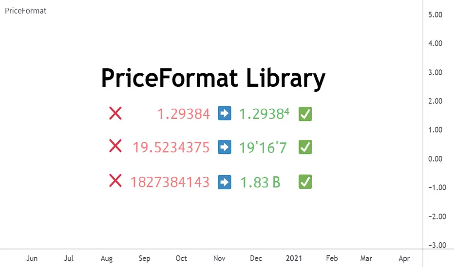
PriceFormatLibrary for automatically converting price values to formatted strings
matching the same format that TradingView uses to display open/high/low/close prices on the chart.
█ OVERVIEW
This library is intended for Pine Coders who are authors of scripts that display numbers onto a user's charts. Typically, 𝚜𝚝𝚛.𝚝𝚘𝚜𝚝𝚛𝚒𝚗𝚐() would be used to convert a number into a string which can be displayed in a label / box / table, but this only works well for values that are formatted as a simple decimal number. The purpose of this library is to provide an easy way to create a formatted string for values which use other types of formats besides the decimal format.
The main functions exported by this library are:
𝚏𝚘𝚛𝚖𝚊𝚝𝙿𝚛𝚒𝚌𝚎() - creates a formatted string from a price value
𝚖𝚎𝚊𝚜𝚞𝚛𝚎𝙿𝚛𝚒𝚌𝚎𝙲𝚑𝚊𝚗𝚐𝚎() - creates a formatted string from the distance between two prices
𝚝𝚘𝚜𝚝𝚛𝚒𝚗𝚐() - an alternative to the built-in 𝚜𝚝𝚛.𝚝𝚘𝚜𝚝𝚛𝚒𝚗𝚐(𝚟𝚊𝚕𝚞𝚎, 𝚏𝚘𝚛𝚖𝚊𝚝)
This library also exports some auxiliary functions which are used under the hood of the previously mentioned functions, but can also be useful to Pine Coders that need fine-tuned control for customized formatting of numeric values:
Functions that determine information about the current chart:
𝚒𝚜𝙵𝚛𝚊𝚌𝚝𝚒𝚘𝚗𝚊𝚕𝙵𝚘𝚛𝚖𝚊𝚝(), 𝚒𝚜𝚅𝚘𝚕𝚞𝚖𝚎𝙵𝚘𝚛𝚖𝚊𝚝(), 𝚒𝚜𝙿𝚎𝚛𝚌𝚎𝚗𝚝𝚊𝚐𝚎𝙵𝚘𝚛𝚖𝚊𝚝(), 𝚒𝚜𝙳𝚎𝚌𝚒𝚖𝚊𝚕𝙵𝚘𝚛𝚖𝚊𝚝(), 𝚒𝚜𝙿𝚒𝚙𝚜𝙵𝚘𝚛𝚖𝚊𝚝()
Functions that convert a 𝚏𝚕𝚘𝚊𝚝 value to a formatted string:
𝚊𝚜𝙳𝚎𝚌𝚒𝚖𝚊𝚕(), 𝚊𝚜𝙿𝚒𝚙𝚜(), 𝚊𝚜𝙵𝚛𝚊𝚌𝚝𝚒𝚘𝚗𝚊𝚕(), 𝚊𝚜𝚅𝚘𝚕𝚞𝚖𝚎()
█ EXAMPLES
• Simple Example
This example shows the simplest way to utilize this library.
//@version=6
indicator("Simple Example")
import n00btraders/PriceFormat/1
var table t = table.new(position.middle_right, 2, 1, bgcolor = color.new(color.blue, 90), force_overlay = true)
if barstate.isfirst
table.cell(t, 0, 0, "Current Price: ", text_color = color.black, text_size = 40)
table.cell(t, 1, 0, text_color = color.blue, text_size = 40)
if barstate.islast
string lastPrice = close.formatPrice() // Simple, easy way to format price
table.cell_set_text(t, 1, 0, lastPrice)
• Complex Example
This example calls all of the main functions and uses their optional arguments.
//@version=6
indicator("Complex Example")
import n00btraders/PriceFormat/1
// Enum values that can be used as optional arguments
precision = input.enum(PriceFormat.Precision.DEFAULT)
language = input.enum(PriceFormat.Language.ENGLISH)
// Main library functions used to create formatted strings
string formattedOpen = open.formatPrice(precision, language, allowPips = true)
string rawOpenPrice = PriceFormat.tostring(open, format.price)
string formattedClose = close.formatPrice(precision, language, allowPips = true)
string rawClosePrice = PriceFormat.tostring(close, format.price)
= PriceFormat.measurePriceChange(open, close, precision, language, allowPips = true)
// Labels to display formatted values on chart
string prices = str.format("Open: {0} ({1}) Close: {2} ({3})", formattedOpen, rawOpenPrice, formattedClose, rawClosePrice)
string change = str.format("Change (close - open): {0} / {1}", distance, ticks)
label.new(chart.point.now(high), prices, yloc = yloc.abovebar, textalign = text.align_left, force_overlay = true)
label.new(chart.point.now(low), change, yloc = yloc.belowbar, style = label.style_label_up, force_overlay = true)
█ NOTES
• Function Descriptions
The library source code uses Markdown for the exported functions. Hover over a function/method call in the Pine Editor to display formatted, detailed information about the function/method.
• Precision Settings
The Precision option in the chart settings can change the format of how prices are displayed on the chart. Since the user's selected choice cannot be known through any Pine built-in variable, this library provides a 𝙿𝚛𝚎𝚌𝚒𝚜𝚒𝚘𝚗 enum that can be used as an optional script input for the user to specify their selected choice.
• Language Settings
The Language option in the user menu can change the decimal/grouping separators in the prices that are displayed on the chart. Since the user's selected choice cannot be known through any Pine built-in variable, this library provides a 𝙻𝚊𝚗𝚐𝚞𝚊𝚐𝚎 enum that can be used as an optional script input for the user to specify their selected choice.
█ EXPORTED FUNCTIONS
method formatPrice(price, precision, language, allowPips)
Formats a price value to match how it would be displayed on the user's current chart.
Namespace types: series float, simple float, input float, const float
Parameters:
price (float) : The value to format.
precision (series Precision) : A Precision.* enum value.
language (series Language) : A Language.* enum value.
allowPips (simple bool) : Whether to allow decimal numbers to display as pips.
Returns: Automatically formatted price string.
measurePriceChange(startPrice, endPrice, precision, language, allowPips)
Measures a change in price in terms of both distance and ticks.
Parameters:
startPrice (float) : The starting price.
endPrice (float) : The ending price.
precision (series Precision) : A Precision.* enum value.
language (series Language) : A Language.* enum value.
allowPips (simple bool) : Whether to allow decimal numbers to display as pips.
Returns: A tuple of formatted strings: .
method tostring(value, format)
Alternative to the Pine `str.tostring(value, format)` built-in function.
Namespace types: series float, simple float, input float, const float
Parameters:
value (float) : (series float) The value to format.
format (string) : (series string) The format string.
Returns: String in the specified format.
isFractionalFormat()
Determines if the default behavior of the chart's price scale is to use a fractional format.
Returns: True if the chart can display prices in fractional format.
isVolumeFormat()
Determines if the default behavior of the chart's price scale is to display prices as volume.
Returns: True if the chart can display prices as volume.
isPercentageFormat()
Determines if the default behavior of the chart's price scale is to display percentages.
Returns: True if the chart can display prices as percentages.
isDecimalFormat()
Determines if the default behavior of the chart's price scale is to use a decimal format.
Returns: True if the chart can display prices in decimal format.
isPipsFormat()
Determines if the current symbol's prices can be displayed as pips.
Returns: True if the chart can display prices as pips.
method asDecimal(value, precision, minTick, decimalSeparator, groupingSeparator, eNotation)
Converts a number to a string in decimal format.
Namespace types: series float, simple float, input float, const float
Parameters:
value (float) : The value to format.
precision (int) : Number of decimal places.
minTick (float) : Minimum tick size.
decimalSeparator (string) : The decimal separator.
groupingSeparator (string) : The thousands separator, aka digit group separator.
eNotation (bool) : Whether the result should use E notation.
Returns: String in decimal format.
method asPips(value, priceScale, minMove, minMove2, decimalSeparator, groupingSeparator)
Converts a number to a string in decimal format with the last digit replaced by a superscript.
Namespace types: series float, simple float, input float, const float
Parameters:
value (float) : The value to format.
priceScale (int) : Price scale.
minMove (int) : Min move.
minMove2 (int) : Min move 2.
decimalSeparator (string) : The decimal separator.
groupingSeparator (string) : The thousands separator, aka digit group separator.
Returns: String in decimal format with an emphasis on the pip value.
method asFractional(value, priceScale, minMove, minMove2, fractionalSeparator1, fractionalSeparator2)
Converts a number to a string in fractional format.
Namespace types: series float, simple float, input float, const float
Parameters:
value (float) : The value to format.
priceScale (int) : Price scale.
minMove (int) : Min move.
minMove2 (int) : Min move 2.
fractionalSeparator1 (string) : The primary fractional separator.
fractionalSeparator2 (string) : The secondary fractional separator.
Returns: String in fractional format.
method asVolume(value, precision, minTick, decimalSeparator, groupingSeparator, spacing)
Converts a number to a string in volume format.
Namespace types: series float, simple float, input float, const float
Parameters:
value (float) : The value to format.
precision (int) : Maximum number of decimal places.
minTick (float) : Minimum tick size.
decimalSeparator (string) : The decimal separator.
groupingSeparator (string) : The thousands separator, aka digit group separator.
spacing (string) : The whitespace separator.
Returns: String in volume format.
LogNormalLibrary "LogNormal"
A collection of functions used to model skewed distributions as log-normal.
Prices are commonly modeled using log-normal distributions (ie. Black-Scholes) because they exhibit multiplicative changes with long tails; skewed exponential growth and high variance. This approach is particularly useful for understanding price behavior and estimating risk, assuming continuously compounding returns are normally distributed.
Because log space analysis is not as direct as using math.log(price) , this library extends the Error Functions library to make working with log-normally distributed data as simple as possible.
- - -
QUICK START
Import library into your project
Initialize model with a mean and standard deviation
Pass model params between methods to compute various properties
var LogNorm model = LN.init(arr.avg(), arr.stdev()) // Assumes the library is imported as LN
var mode = model.mode()
Outputs from the model can be adjusted to better fit the data.
var Quantile data = arr.quantiles()
var more_accurate_mode = mode.fit(model, data) // Fits value from model to data
Inputs to the model can also be adjusted to better fit the data.
datum = 123.45
model_equivalent_datum = datum.fit(data, model) // Fits value from data to the model
area_from_zero_to_datum = model.cdf(model_equivalent_datum)
- - -
TYPES
There are two requisite UDTs: LogNorm and Quantile . They are used to pass parameters between functions and are set automatically (see Type Management ).
LogNorm
Object for log space parameters and linear space quantiles .
Fields:
mu (float) : Log space mu ( µ ).
sigma (float) : Log space sigma ( σ ).
variance (float) : Log space variance ( σ² ).
quantiles (Quantile) : Linear space quantiles.
Quantile
Object for linear quantiles, most similar to a seven-number summary .
Fields:
Q0 (float) : Smallest Value
LW (float) : Lower Whisker Endpoint
LC (float) : Lower Whisker Crosshatch
Q1 (float) : First Quartile
Q2 (float) : Second Quartile
Q3 (float) : Third Quartile
UC (float) : Upper Whisker Crosshatch
UW (float) : Upper Whisker Endpoint
Q4 (float) : Largest Value
IQR (float) : Interquartile Range
MH (float) : Midhinge
TM (float) : Trimean
MR (float) : Mid-Range
- - -
TYPE MANAGEMENT
These functions reliably initialize and update the UDTs. Because parameterization is interdependent, avoid setting the LogNorm and Quantile fields directly .
init(mean, stdev, variance)
Initializes a LogNorm object.
Parameters:
mean (float) : Linearly measured mean.
stdev (float) : Linearly measured standard deviation.
variance (float) : Linearly measured variance.
Returns: LogNorm Object
set(ln, mean, stdev, variance)
Transforms linear measurements into log space parameters for a LogNorm object.
Parameters:
ln (LogNorm) : Object containing log space parameters.
mean (float) : Linearly measured mean.
stdev (float) : Linearly measured standard deviation.
variance (float) : Linearly measured variance.
Returns: LogNorm Object
quantiles(arr)
Gets empirical quantiles from an array of floats.
Parameters:
arr (array) : Float array object.
Returns: Quantile Object
- - -
DESCRIPTIVE STATISTICS
Using only the initialized LogNorm parameters, these functions compute a model's central tendency and standardized moments.
mean(ln)
Computes the linear mean from log space parameters.
Parameters:
ln (LogNorm) : Object containing log space parameters.
Returns: Between 0 and ∞
median(ln)
Computes the linear median from log space parameters.
Parameters:
ln (LogNorm) : Object containing log space parameters.
Returns: Between 0 and ∞
mode(ln)
Computes the linear mode from log space parameters.
Parameters:
ln (LogNorm) : Object containing log space parameters.
Returns: Between 0 and ∞
variance(ln)
Computes the linear variance from log space parameters.
Parameters:
ln (LogNorm) : Object containing log space parameters.
Returns: Between 0 and ∞
skewness(ln)
Computes the linear skewness from log space parameters.
Parameters:
ln (LogNorm) : Object containing log space parameters.
Returns: Between 0 and ∞
kurtosis(ln, excess)
Computes the linear kurtosis from log space parameters.
Parameters:
ln (LogNorm) : Object containing log space parameters.
excess (bool) : Excess Kurtosis (true) or regular Kurtosis (false).
Returns: Between 0 and ∞
hyper_skewness(ln)
Computes the linear hyper skewness from log space parameters.
Parameters:
ln (LogNorm) : Object containing log space parameters.
Returns: Between 0 and ∞
hyper_kurtosis(ln, excess)
Computes the linear hyper kurtosis from log space parameters.
Parameters:
ln (LogNorm) : Object containing log space parameters.
excess (bool) : Excess Hyper Kurtosis (true) or regular Hyper Kurtosis (false).
Returns: Between 0 and ∞
- - -
DISTRIBUTION FUNCTIONS
These wrap Gaussian functions to make working with model space more direct. Because they are contained within a log-normal library, they describe estimations relative to a log-normal curve, even though they fundamentally measure a Gaussian curve.
pdf(ln, x, empirical_quantiles)
A Probability Density Function estimates the probability density . For clarity, density is not a probability .
Parameters:
ln (LogNorm) : Object of log space parameters.
x (float) : Linear X coordinate for which a density will be estimated.
empirical_quantiles (Quantile) : Quantiles as observed in the data (optional).
Returns: Between 0 and ∞
cdf(ln, x, precise)
A Cumulative Distribution Function estimates the area under a Log-Normal curve between Zero and a linear X coordinate.
Parameters:
ln (LogNorm) : Object of log space parameters.
x (float) : Linear X coordinate .
precise (bool) : Double precision (true) or single precision (false).
Returns: Between 0 and 1
ccdf(ln, x, precise)
A Complementary Cumulative Distribution Function estimates the area under a Log-Normal curve between a linear X coordinate and Infinity.
Parameters:
ln (LogNorm) : Object of log space parameters.
x (float) : Linear X coordinate .
precise (bool) : Double precision (true) or single precision (false).
Returns: Between 0 and 1
cdfinv(ln, a, precise)
An Inverse Cumulative Distribution Function reverses the Log-Normal cdf() by estimating the linear X coordinate from an area.
Parameters:
ln (LogNorm) : Object of log space parameters.
a (float) : Normalized area .
precise (bool) : Double precision (true) or single precision (false).
Returns: Between 0 and ∞
ccdfinv(ln, a, precise)
An Inverse Complementary Cumulative Distribution Function reverses the Log-Normal ccdf() by estimating the linear X coordinate from an area.
Parameters:
ln (LogNorm) : Object of log space parameters.
a (float) : Normalized area .
precise (bool) : Double precision (true) or single precision (false).
Returns: Between 0 and ∞
cdfab(ln, x1, x2, precise)
A Cumulative Distribution Function from A to B estimates the area under a Log-Normal curve between two linear X coordinates (A and B).
Parameters:
ln (LogNorm) : Object of log space parameters.
x1 (float) : First linear X coordinate .
x2 (float) : Second linear X coordinate .
precise (bool) : Double precision (true) or single precision (false).
Returns: Between 0 and 1
ott(ln, x, precise)
A One-Tailed Test transforms a linear X coordinate into an absolute Z Score before estimating the area under a Log-Normal curve between Z and Infinity.
Parameters:
ln (LogNorm) : Object of log space parameters.
x (float) : Linear X coordinate .
precise (bool) : Double precision (true) or single precision (false).
Returns: Between 0 and 0.5
ttt(ln, x, precise)
A Two-Tailed Test transforms a linear X coordinate into symmetrical ± Z Scores before estimating the area under a Log-Normal curve from Zero to -Z, and +Z to Infinity.
Parameters:
ln (LogNorm) : Object of log space parameters.
x (float) : Linear X coordinate .
precise (bool) : Double precision (true) or single precision (false).
Returns: Between 0 and 1
ottinv(ln, a, precise)
An Inverse One-Tailed Test reverses the Log-Normal ott() by estimating a linear X coordinate for the right tail from an area.
Parameters:
ln (LogNorm) : Object of log space parameters.
a (float) : Half a normalized area .
precise (bool) : Double precision (true) or single precision (false).
Returns: Between 0 and ∞
tttinv(ln, a, precise)
An Inverse Two-Tailed Test reverses the Log-Normal ttt() by estimating two linear X coordinates from an area.
Parameters:
ln (LogNorm) : Object of log space parameters.
a (float) : Normalized area .
precise (bool) : Double precision (true) or single precision (false).
Returns: Linear space tuple :
- - -
UNCERTAINTY
Model-based measures of uncertainty, information, and risk.
sterr(sample_size, fisher_info)
The standard error of a sample statistic.
Parameters:
sample_size (float) : Number of observations.
fisher_info (float) : Fisher information.
Returns: Between 0 and ∞
surprisal(p, base)
Quantifies the information content of a single event.
Parameters:
p (float) : Probability of the event .
base (float) : Logarithmic base (optional).
Returns: Between 0 and ∞
entropy(ln, base)
Computes the differential entropy (average surprisal).
Parameters:
ln (LogNorm) : Object of log space parameters.
base (float) : Logarithmic base (optional).
Returns: Between 0 and ∞
perplexity(ln, base)
Computes the average number of distinguishable outcomes from the entropy.
Parameters:
ln (LogNorm)
base (float) : Logarithmic base used for Entropy (optional).
Returns: Between 0 and ∞
value_at_risk(ln, p, precise)
Estimates a risk threshold under normal market conditions for a given confidence level.
Parameters:
ln (LogNorm) : Object of log space parameters.
p (float) : Probability threshold, aka. the confidence level .
precise (bool) : Double precision (true) or single precision (false).
Returns: Between 0 and ∞
value_at_risk_inv(ln, value_at_risk, precise)
Reverses the value_at_risk() by estimating the confidence level from the risk threshold.
Parameters:
ln (LogNorm) : Object of log space parameters.
value_at_risk (float) : Value at Risk.
precise (bool) : Double precision (true) or single precision (false).
Returns: Between 0 and 1
conditional_value_at_risk(ln, p, precise)
Estimates the average loss beyond a confidence level, aka. expected shortfall.
Parameters:
ln (LogNorm) : Object of log space parameters.
p (float) : Probability threshold, aka. the confidence level .
precise (bool) : Double precision (true) or single precision (false).
Returns: Between 0 and ∞
conditional_value_at_risk_inv(ln, conditional_value_at_risk, precise)
Reverses the conditional_value_at_risk() by estimating the confidence level of an average loss.
Parameters:
ln (LogNorm) : Object of log space parameters.
conditional_value_at_risk (float) : Conditional Value at Risk.
precise (bool) : Double precision (true) or single precision (false).
Returns: Between 0 and 1
partial_expectation(ln, x, precise)
Estimates the partial expectation of a linear X coordinate.
Parameters:
ln (LogNorm) : Object of log space parameters.
x (float) : Linear X coordinate .
precise (bool) : Double precision (true) or single precision (false).
Returns: Between 0 and µ
partial_expectation_inv(ln, partial_expectation, precise)
Reverses the partial_expectation() by estimating a linear X coordinate.
Parameters:
ln (LogNorm) : Object of log space parameters.
partial_expectation (float) : Partial Expectation .
precise (bool) : Double precision (true) or single precision (false).
Returns: Between 0 and ∞
conditional_expectation(ln, x, precise)
Estimates the conditional expectation of a linear X coordinate.
Parameters:
ln (LogNorm) : Object of log space parameters.
x (float) : Linear X coordinate .
precise (bool) : Double precision (true) or single precision (false).
Returns: Between X and ∞
conditional_expectation_inv(ln, conditional_expectation, precise)
Reverses the conditional_expectation by estimating a linear X coordinate.
Parameters:
ln (LogNorm) : Object of log space parameters.
conditional_expectation (float) : Conditional Expectation .
precise (bool) : Double precision (true) or single precision (false).
Returns: Between 0 and ∞
fisher(ln, log)
Computes the Fisher Information Matrix for the distribution, not a linear X coordinate.
Parameters:
ln (LogNorm) : Object of log space parameters.
log (bool) : Sets if the matrix should be in log (true) or linear (false) space.
Returns: FIM for the distribution
fisher(ln, x, log)
Computes the Fisher Information Matrix for a linear X coordinate, not the distribution itself.
Parameters:
ln (LogNorm) : Object of log space parameters.
x (float) : Linear X coordinate .
log (bool) : Sets if the matrix should be in log (true) or linear (false) space.
Returns: FIM for the linear X coordinate
confidence_interval(ln, x, sample_size, confidence, precise)
Estimates a confidence interval for a linear X coordinate.
Parameters:
ln (LogNorm) : Object of log space parameters.
x (float) : Linear X coordinate .
sample_size (float) : Number of observations.
confidence (float) : Confidence level .
precise (bool) : Double precision (true) or single precision (false).
Returns: CI for the linear X coordinate
- - -
CURVE FITTING
An overloaded function that helps transform values between spaces. The primary function uses quantiles, and the overloads wrap the primary function to make working with LogNorm more direct.
fit(x, a, b)
Transforms X coordinate between spaces A and B.
Parameters:
x (float) : Linear X coordinate from space A .
a (LogNorm | Quantile | array) : LogNorm, Quantile, or float array.
b (LogNorm | Quantile | array) : LogNorm, Quantile, or float array.
Returns: Adjusted X coordinate
- - -
EXPORTED HELPERS
Small utilities to simplify extensibility.
z_score(ln, x)
Converts a linear X coordinate into a Z Score.
Parameters:
ln (LogNorm) : Object of log space parameters.
x (float) : Linear X coordinate.
Returns: Between -∞ and +∞
x_coord(ln, z)
Converts a Z Score into a linear X coordinate.
Parameters:
ln (LogNorm) : Object of log space parameters.
z (float) : Standard normal Z Score.
Returns: Between 0 and ∞
iget(arr, index)
Gets an interpolated value of a pseudo -element (fictional element between real array elements). Useful for quantile mapping.
Parameters:
arr (array) : Float array object.
index (float) : Index of the pseudo element.
Returns: Interpolated value of the arrays pseudo element.

RiskMetrics█ OVERVIEW
This library is a tool for Pine programmers that provides functions for calculating risk-adjusted performance metrics on periodic price returns. The calculations used by this library's functions closely mirror those the Broker Emulator uses to calculate strategy performance metrics (e.g., Sharpe and Sortino ratios) without depending on strategy-specific functionality.
█ CONCEPTS
Returns, risk, and volatility
The return on an investment is the relative gain or loss over a period, often expressed as a percentage. Investment returns can originate from several sources, including capital gains, dividends, and interest income. Many investors seek the highest returns possible in the quest for profit. However, prudent investing and trading entails evaluating such returns against the associated risks (i.e., the uncertainty of returns and the potential for financial losses) for a clearer perspective on overall performance and sustainability.
One way investors and analysts assess the risk of an investment is by analyzing its volatility , i.e., the statistical dispersion of historical returns. Investors often use volatility in risk estimation because it provides a quantifiable way to gauge the expected extent of fluctuation in returns. Elevated volatility implies heightened uncertainty in the market, which suggests higher expected risk. Conversely, low volatility implies relatively stable returns with relatively minimal fluctuations, thus suggesting lower expected risk. Several risk-adjusted performance metrics utilize volatility in their calculations for this reason.
Risk-free rate
The risk-free rate represents the rate of return on a hypothetical investment carrying no risk of financial loss. This theoretical rate provides a benchmark for comparing the returns on a risky investment and evaluating whether its excess returns justify the risks. If an investment's returns are at or below the theoretical risk-free rate or the risk premium is below a desired amount, it may suggest that the returns do not compensate for the extra risk, which might be a call to reassess the investment.
Since the risk-free rate is a theoretical concept, investors often utilize proxies for the rate in practice, such as Treasury bills and other government bonds. Conventionally, analysts consider such instruments "risk-free" for a domestic holder, as they are a form of government obligation with a low perceived likelihood of default.
The average yield on short-term Treasury bills, influenced by economic conditions, monetary policies, and inflation expectations, has historically hovered around 2-3% over the long term. This range also aligns with central banks' inflation targets. As such, one may interpret a value within this range as a minimum proxy for the risk-free rate, as it may correspond to the minimum rate required to maintain purchasing power over time.
The built-in Sharpe and Sortino ratios that strategies calculate and display in the Performance Summary tab use a default risk-free rate of 2%, and the metrics in this library's example code use the same default rate. Users can adjust this value to fit their analysis needs.
Risk-adjusted performance
Risk-adjusted performance metrics gauge the effectiveness of an investment by considering its returns relative to the perceived risk. They aim to provide a more well-rounded picture of performance by factoring in the level of risk taken to achieve returns. Investors can utilize such metrics to help determine whether the returns from an investment justify the risks and make informed decisions.
The two most commonly used risk-adjusted performance metrics are the Sharpe ratio and the Sortino ratio.
1. Sharpe ratio
The Sharpe ratio , developed by Nobel laureate William F. Sharpe, measures the performance of an investment compared to a theoretically risk-free asset, adjusted for the investment risk. The ratio uses the following formula:
Sharpe Ratio = (𝑅𝑎 − 𝑅𝑓) / 𝜎𝑎
Where:
• 𝑅𝑎 = Average return of the investment
• 𝑅𝑓 = Theoretical risk-free rate of return
• 𝜎𝑎 = Standard deviation of the investment's returns (volatility)
A higher Sharpe ratio indicates a more favorable risk-adjusted return, as it signifies that the investment produced higher excess returns per unit of increase in total perceived risk.
2. Sortino ratio
The Sortino ratio is a modified form of the Sharpe ratio that only considers downside volatility , i.e., the volatility of returns below the theoretical risk-free benchmark. Although it shares close similarities with the Sharpe ratio, it can produce very different values, especially when the returns do not have a symmetrical distribution, since it does not penalize upside and downside volatility equally. The ratio uses the following formula:
Sortino Ratio = (𝑅𝑎 − 𝑅𝑓) / 𝜎𝑑
Where:
• 𝑅𝑎 = Average return of the investment
• 𝑅𝑓 = Theoretical risk-free rate of return
• 𝜎𝑑 = Downside deviation (standard deviation of negative excess returns, or downside volatility)
The Sortino ratio offers an alternative perspective on an investment's return-generating efficiency since it does not consider upside volatility in its calculation. A higher Sortino ratio signifies that the investment produced higher excess returns per unit of increase in perceived downside risk.
█ CALCULATIONS
Return period detection
Calculating risk-adjusted performance metrics requires collecting returns across several periods of a given size. Analysts may use different period sizes based on the context and their preferences. However, two widely used standards are monthly or daily periods, depending on the available data and the investment's duration. The built-in ratios displayed in the Strategy Tester utilize returns from either monthly or daily periods in their calculations based on the following logic:
• Use monthly returns if the history of closed trades spans at least two months.
• Use daily returns if the trades span at least two days but less than two months.
• Do not calculate the ratios if the trade data spans fewer than two days.
This library's `detectPeriod()` function applies related logic to available chart data rather than trade data to determine which period is appropriate:
• It returns true if the chart's data spans at least two months, indicating that it's sufficient to use monthly periods.
• It returns false if the chart's data spans at least two days but not two months, suggesting the use of daily periods.
• It returns na if the length of the chart's data covers less than two days, signifying that the data is insufficient for meaningful ratio calculations.
It's important to note that programmers should only call `detectPeriod()` from a script's global scope or within the outermost scope of a function called from the global scope, as it requires the time value from the first bar to accurately measure the amount of time covered by the chart's data.
Collecting periodic returns
This library's `getPeriodicReturns()` function tracks price return data within monthly or daily periods and stores the periodic values in an array . It uses a `detectPeriod()` call as the condition to determine whether each element in the array represents the return over a monthly or daily period.
The `getPeriodicReturns()` function has two overloads. The first overload requires two arguments and outputs an array of monthly or daily returns for use in the `sharpe()` and `sortino()` methods. To calculate these returns:
1. The `percentChange` argument should be a series that represents percentage gains or losses. The values can be bar-to-bar return percentages on the chart timeframe or percentages requested from a higher timeframe.
2. The function compounds all non-na `percentChange` values within each monthly or daily period to calculate the period's total return percentage. When the `percentChange` represents returns from a higher timeframe, ensure the requested data includes gaps to avoid compounding redundant values.
3. After a period ends, the function queues the compounded return into the array , removing the oldest element from the array when its size exceeds the `maxPeriods` argument.
The resulting array represents the sequence of closed returns over up to `maxPeriods` months or days, depending on the available data.
The second overload of the function includes an additional `benchmark` parameter. Unlike the first overload, this version tracks and collects differences between the `percentChange` and the specified `benchmark` values. The resulting array represents the sequence of excess returns over up to `maxPeriods` months or days. Passing this array to the `sharpe()` and `sortino()` methods calculates generalized Information ratios , which represent the risk-adjustment performance of a sequence of returns compared to a risky benchmark instead of a risk-free rate. For consistency, ensure the non-na times of the `benchmark` values align with the times of the `percentChange` values.
Ratio methods
This library's `sharpe()` and `sortino()` methods respectively calculate the Sharpe and Sortino ratios based on an array of returns compared to a specified annual benchmark. Both methods adjust the annual benchmark based on the number of periods per year to suit the frequency of the returns:
• If the method call does not include a `periodsPerYear` argument, it uses `detectPeriod()` to determine whether the returns represent monthly or daily values based on the chart's history. If monthly, the method divides the `annualBenchmark` value by 12. If daily, it divides the value by 365.
• If the method call does specify a `periodsPerYear` argument, the argument's value supersedes the automatic calculation, facilitating custom benchmark adjustments, such as dividing by 252 when analyzing collected daily stock returns.
When the array passed to these methods represents a sequence of excess returns , such as the result from the second overload of `getPeriodicReturns()`, use an `annualBenchmark` value of 0 to avoid comparing those excess returns to a separate rate.
By default, these methods only calculate the ratios on the last available bar to minimize their resource usage. Users can override this behavior with the `forceCalc` parameter. When the value is true , the method calculates the ratio on each call if sufficient data is available, regardless of the bar index.
Look first. Then leap.
█ FUNCTIONS & METHODS
This library contains the following functions:
detectPeriod()
Determines whether the chart data has sufficient coverage to use monthly or daily returns
for risk metric calculations.
Returns: (bool) `true` if the period spans more than two months, `false` if it otherwise spans more
than two days, and `na` if the data is insufficient.
getPeriodicReturns(percentChange, maxPeriods)
(Overload 1 of 2) Tracks periodic return percentages and queues them into an array for ratio
calculations. The span of the chart's historical data determines whether the function uses
daily or monthly periods in its calculations. If the chart spans more than two months,
it uses "1M" periods. Otherwise, if the chart spans more than two days, it uses "1D"
periods. If the chart covers less than two days, it does not store changes.
Parameters:
percentChange (float) : (series float) The change percentage. The function compounds non-na values from each
chart bar within monthly or daily periods to calculate the periodic changes.
maxPeriods (simple int) : (simple int) The maximum number of periodic returns to store in the returned array.
Returns: (array) An array containing the overall percentage changes for each period, limited
to the maximum specified by `maxPeriods`.
getPeriodicReturns(percentChange, benchmark, maxPeriods)
(Overload 2 of 2) Tracks periodic excess return percentages and queues the values into an
array. The span of the chart's historical data determines whether the function uses
daily or monthly periods in its calculations. If the chart spans more than two months,
it uses "1M" periods. Otherwise, if the chart spans more than two days, it uses "1D"
periods. If the chart covers less than two days, it does not store changes.
Parameters:
percentChange (float) : (series float) The change percentage. The function compounds non-na values from each
chart bar within monthly or daily periods to calculate the periodic changes.
benchmark (float) : (series float) The benchmark percentage to compare against `percentChange` values.
The function compounds non-na values from each bar within monthly or
daily periods and subtracts the results from the compounded `percentChange` values to
calculate the excess returns. For consistency, ensure this series has a similar history
length to the `percentChange` with aligned non-na value times.
maxPeriods (simple int) : (simple int) The maximum number of periodic excess returns to store in the returned array.
Returns: (array) An array containing monthly or daily excess returns, limited
to the maximum specified by `maxPeriods`.
method sharpeRatio(returnsArray, annualBenchmark, forceCalc, periodsPerYear)
Calculates the Sharpe ratio for an array of periodic returns.
Callable as a method or a function.
Namespace types: array
Parameters:
returnsArray (array) : (array) An array of periodic return percentages, e.g., returns over monthly or
daily periods.
annualBenchmark (float) : (series float) The annual rate of return to compare against `returnsArray` values. When
`periodsPerYear` is `na`, the function divides this value by 12 to calculate a
monthly benchmark if the chart's data spans at least two months or 365 for a daily
benchmark if the data otherwise spans at least two days. If `periodsPerYear`
has a specified value, the function divides the rate by that value instead.
forceCalc (bool) : (series bool) If `true`, calculates the ratio on every call. Otherwise, ratio calculation
only occurs on the last available bar. Optional. The default is `false`.
periodsPerYear (simple int) : (simple int) If specified, divides the annual rate by this value instead of the value
determined by the time span of the chart's data.
Returns: (float) The Sharpe ratio, which estimates the excess return per unit of total volatility.
method sortinoRatio(returnsArray, annualBenchmark, forceCalc, periodsPerYear)
Calculates the Sortino ratio for an array of periodic returns.
Callable as a method or a function.
Namespace types: array
Parameters:
returnsArray (array) : (array) An array of periodic return percentages, e.g., returns over monthly or
daily periods.
annualBenchmark (float) : (series float) The annual rate of return to compare against `returnsArray` values. When
`periodsPerYear` is `na`, the function divides this value by 12 to calculate a
monthly benchmark if the chart's data spans at least two months or 365 for a daily
benchmark if the data otherwise spans at least two days. If `periodsPerYear`
has a specified value, the function divides the rate by that value instead.
forceCalc (bool) : (series bool) If `true`, calculates the ratio on every call. Otherwise, ratio calculation
only occurs on the last available bar. Optional. The default is `false`.
periodsPerYear (simple int) : (simple int) If specified, divides the annual rate by this value instead of the value
determined by the time span of the chart's data.
Returns: (float) The Sortino ratio, which estimates the excess return per unit of downside
volatility.

analytics_tablesLibrary "analytics_tables"
📝 Description
This library provides the implementation of several performance-related statistics and metrics, presented in the form of tables.
The metrics shown in the afforementioned tables where developed during the past years of my in-depth analalysis of various strategies in an atempt to reason about the performance of each strategy.
The visualization and some statistics where inspired by the existing implementations of the "Seasonality" script, and the performance matrix implementations of @QuantNomad and @ZenAndTheArtOfTrading scripts.
While this library is meant to be used by my strategy framework "Template Trailing Strategy (Backtester)" script, I wrapped it in a library hoping this can be usefull for other community strategy scripts that will be released in the future.
🤔 How to Guide
To use the functionality this library provides in your script you have to import it first!
Copy the import statement of the latest release by pressing the copy button below and then paste it into your script. Give a short name to this library so you can refer to it later on. The import statement should look like this:
import jason5480/analytics_tables/1 as ant
There are three types of tables provided by this library in the initial release. The stats table the metrics table and the seasonality table.
Each one shows different kinds of performance statistics.
The table UDT shall be initialized once using the `init()` method.
They can be updated using the `update()` method where the updated data UDT object shall be passed.
The data UDT can also initialized and get updated on demend depending on the use case
A code example for the StatsTable is the following:
var ant.StatsData statsData = ant.StatsData.new()
statsData.update(SideStats.new(), SideStats.new(), 0)
if (barstate.islastconfirmedhistory or (barstate.isrealtime and barstate.isconfirmed))
var statsTable = ant.StatsTable.new().init(ant.getTablePos('TOP', 'RIGHT'))
statsTable.update(statsData)
A code example for the MetricsTable is the following:
var ant.StatsData statsData = ant.StatsData.new()
statsData.update(ant.SideStats.new(), ant.SideStats.new(), 0)
if (barstate.islastconfirmedhistory or (barstate.isrealtime and barstate.isconfirmed))
var metricsTable = ant.MetricsTable.new().init(ant.getTablePos('BOTTOM', 'RIGHT'))
metricsTable.update(statsData, 10)
A code example for the SeasonalityTable is the following:
var ant.SeasonalData seasonalData = ant.SeasonalData.new().init(Seasonality.monthOfYear)
seasonalData.update()
if (barstate.islastconfirmedhistory or (barstate.isrealtime and barstate.isconfirmed))
var seasonalTable = ant.SeasonalTable.new().init(seasonalData, ant.getTablePos('BOTTOM', 'LEFT'))
seasonalTable.update(seasonalData)
🏋️♂️ Please refer to the "EXAMPLE" regions of the script for more advanced and up to date code examples!
Special thanks to @Mrcrbw for the proposal to develop this library and @DCNeu for the constructive feedback 🏆.
getTablePos(ypos, xpos)
Get table position compatible string
Parameters:
ypos (simple string) : The position on y axise
xpos (simple string) : The position on x axise
Returns: The position to be passed to the table
method init(this, pos, height, width, positiveTxtColor, negativeTxtColor, neutralTxtColor, positiveBgColor, negativeBgColor, neutralBgColor)
Initialize the stats table object with the given colors in the given position
Namespace types: StatsTable
Parameters:
this (StatsTable) : The stats table object
pos (simple string) : The table position string
height (simple float) : The height of the table as a percentage of the charts height. By default, 0 auto-adjusts the height based on the text inside the cells
width (simple float) : The width of the table as a percentage of the charts height. By default, 0 auto-adjusts the width based on the text inside the cells
positiveTxtColor (simple color) : The text color when positive
negativeTxtColor (simple color) : The text color when negative
neutralTxtColor (simple color) : The text color when neutral
positiveBgColor (simple color) : The background color with transparency when positive
negativeBgColor (simple color) : The background color with transparency when negative
neutralBgColor (simple color) : The background color with transparency when neutral
method init(this, pos, height, width, neutralBgColor)
Initialize the metrics table object with the given colors in the given position
Namespace types: MetricsTable
Parameters:
this (MetricsTable) : The metrics table object
pos (simple string) : The table position string
height (simple float) : The height of the table as a percentage of the charts height. By default, 0 auto-adjusts the height based on the text inside the cells
width (simple float) : The width of the table as a percentage of the charts width. By default, 0 auto-adjusts the width based on the text inside the cells
neutralBgColor (simple color) : The background color with transparency when neutral
method init(this, seas)
Initialize the seasonal data
Namespace types: SeasonalData
Parameters:
this (SeasonalData) : The seasonal data object
seas (simple Seasonality) : The seasonality of the matrix data
method init(this, data, pos, maxNumOfYears, height, width, extended, neutralTxtColor, neutralBgColor)
Initialize the seasonal table object with the given colors in the given position
Namespace types: SeasonalTable
Parameters:
this (SeasonalTable) : The seasonal table object
data (SeasonalData) : The seasonality data of the table
pos (simple string) : The table position string
maxNumOfYears (simple int) : The maximum number of years that fit into the table
height (simple float) : The height of the table as a percentage of the charts height. By default, 0 auto-adjusts the height based on the text inside the cells
width (simple float) : The width of the table as a percentage of the charts width. By default, 0 auto-adjusts the width based on the text inside the cells
extended (simple bool) : The seasonal table with extended columns for performance
neutralTxtColor (simple color) : The text color when neutral
neutralBgColor (simple color) : The background color with transparency when neutral
method update(this, wins, losses, numOfInconclusiveExits)
Update the strategy info data of the strategy
Namespace types: StatsData
Parameters:
this (StatsData) : The strategy statistics object
wins (SideStats)
losses (SideStats)
numOfInconclusiveExits (int) : The number of inconclusive trades
method update(this, stats, positiveTxtColor, negativeTxtColor, negativeBgColor, neutralBgColor)
Update the stats table object with the given data
Namespace types: StatsTable
Parameters:
this (StatsTable) : The stats table object
stats (StatsData) : The stats data to update the table
positiveTxtColor (simple color) : The text color when positive
negativeTxtColor (simple color) : The text color when negative
negativeBgColor (simple color) : The background color with transparency when negative
neutralBgColor (simple color) : The background color with transparency when neutral
method update(this, stats, buyAndHoldPerc, positiveTxtColor, negativeTxtColor, positiveBgColor, negativeBgColor)
Update the metrics table object with the given data
Namespace types: MetricsTable
Parameters:
this (MetricsTable) : The metrics table object
stats (StatsData) : The stats data to update the table
buyAndHoldPerc (float) : The buy and hold percetage
positiveTxtColor (simple color) : The text color when positive
negativeTxtColor (simple color) : The text color when negative
positiveBgColor (simple color) : The background color with transparency when positive
negativeBgColor (simple color) : The background color with transparency when negative
method update(this)
Update the seasonal data based on the season and eon timeframe
Namespace types: SeasonalData
Parameters:
this (SeasonalData) : The seasonal data object
method update(this, data, positiveTxtColor, negativeTxtColor, neutralTxtColor, positiveBgColor, negativeBgColor, neutralBgColor, timeBgColor)
Update the seasonal table object with the given data
Namespace types: SeasonalTable
Parameters:
this (SeasonalTable) : The seasonal table object
data (SeasonalData) : The seasonal cell data to update the table
positiveTxtColor (simple color) : The text color when positive
negativeTxtColor (simple color) : The text color when negative
neutralTxtColor (simple color) : The text color when neutral
positiveBgColor (simple color) : The background color with transparency when positive
negativeBgColor (simple color) : The background color with transparency when negative
neutralBgColor (simple color) : The background color with transparency when neutral
timeBgColor (simple color) : The background color of the time gradient
SideStats
Object that represents the strategy statistics data of one side win or lose
Fields:
numOf (series int)
sumFreeProfit (series float)
freeProfitStDev (series float)
sumProfit (series float)
profitStDev (series float)
sumGain (series float)
gainStDev (series float)
avgQuantityPerc (series float)
avgCapitalRiskPerc (series float)
avgTPExecutedCount (series float)
avgRiskRewardRatio (series float)
maxStreak (series int)
StatsTable
Object that represents the stats table
Fields:
table (series table) : The actual table
rows (series int) : The number of rows of the table
columns (series int) : The number of columns of the table
StatsData
Object that represents the statistics data of the strategy
Fields:
wins (SideStats)
losses (SideStats)
numOfInconclusiveExits (series int)
avgFreeProfitStr (series string)
freeProfitStDevStr (series string)
lossFreeProfitStDevStr (series string)
avgProfitStr (series string)
profitStDevStr (series string)
lossProfitStDevStr (series string)
avgQuantityStr (series string)
MetricsTable
Object that represents the metrics table
Fields:
table (series table) : The actual table
rows (series int) : The number of rows of the table
columns (series int) : The number of columns of the table
SeasonalData
Object that represents the seasonal table dynamic data
Fields:
seasonality (series Seasonality)
eonToMatrixRow (map)
numOfEons (series int)
mostRecentMatrixRow (series int)
balances (matrix)
returnPercs (matrix)
maxDDs (matrix)
eonReturnPercs (array)
eonCAGRs (array)
eonMaxDDs (array)
SeasonalTable
Object that represents the seasonal table
Fields:
table (series table) : The actual table
headRows (series int) : The number of head rows of the table
headColumns (series int) : The number of head columns of the table
eonRows (series int) : The number of eon rows of the table
seasonColumns (series int) : The number of season columns of the table
statsRows (series int)
statsColumns (series int) : The number of stats columns of the table
rows (series int) : The number of rows of the table
columns (series int) : The number of columns of the table
extended (series bool) : Whether the table has additional performance statistics

FiniteStateMachine🟩 OVERVIEW
A flexible framework for creating, testing and implementing a Finite State Machine (FSM) in your script. FSMs use rules to control how states change in response to events.
This is the first Finite State Machine library on TradingView and it's quite a different way to think about your script's logic. Advantages of using this vs hardcoding all your logic include:
• Explicit logic : You can see all rules easily side-by-side.
• Validation : Tables show your rules and validation results right on the chart.
• Dual approach : Simple matrix for straightforward transitions; map implementation for concurrent scenarios. You can combine them for complex needs.
• Type safety : Shows how to use enums for robustness while maintaining string compatibility.
• Real-world examples : Includes both conceptual (traffic lights) and practical (trading strategy) demonstrations.
• Priority control : Explicit control over which rules take precedence when multiple conditions are met.
• Wildcard system : Flexible pattern matching for states and events.
The library seems complex, but it's not really. Your conditions, events, and their potential interactions are complex. The FSM makes them all explicit, which is some work. However, like all "good" pain in life, this is front-loaded, and *saves* pain later, in the form of unintended interactions and bugs that are very hard to find and fix.
🟩 SIMPLE FSM (MATRIX-BASED)
The simple FSM uses a matrix to define transition rules with the structure: state > event > state. We look up the current state, check if the event in that row matches, and if it does, output the resulting state.
Each row in the matrix defines one rule, and the first matching row, counting from the top down, is applied.
A limitation of this method is that you can supply only ONE event.
You can design layered rules using widlcards. Use an empty string "" or the special string "ANY" for any state or event wildcard.
The matrix FSM is foruse where you have clear, sequential state transitions triggered by single events. Think traffic lights, or any logic where only one thing can happen at a time.
The demo for this FSM is of traffic lights.
🟩 CONCURRENT FSM (MAP-BASED)
The map FSM uses a more complex structure where each state is a key in the map, and its value is an array of event rules. Each rule maps a named condition to an output (event or next state).
This FSM can handle multiple conditions simultaneously. Rules added first have higher priority.
Adding more rules to existing states combines the entries in the map (if you use the supplied helper function) rather than overwriting them.
This FSM is for more complex scenarios where multiple conditions can be true simultaneously, and you need to control which takes precedence. Like trading strategies, or any system with concurrent conditions.
The demo for this FSM is a trading strategy.
🟩 HOW TO USE
Pine Script libraries contain reusable code for importing into indicators. You do not need to copy any code out of here. Just import the library and call the function you want.
For example, for version 1 of this library, import it like this:
import SimpleCryptoLife/FiniteStateMachine/1
See the EXAMPLE USAGE sections within the library for examples of calling the functions.
For more information on libraries and incorporating them into your scripts, see the Libraries section of the Pine Script User Manual.
🟩 TECHNICAL IMPLEMENTATION
Both FSM implementations support wildcards using blank strings "" or the special string "ANY". Wildcards match in this priority order:
• Exact state + exact event match
• Exact state + empty event (event wildcard)
• Empty state + exact event (state wildcard)
• Empty state + empty event (full wildcard)
When multiple rules match the same state + event combination, the FIRST rule encountered takes priority. In the matrix FSM, this means row order determines priority. In the map FSM, it's the order you add rules to each state.
The library uses user-defined types for the map FSM:
• o_eventRule : Maps a condition name to an output
• o_eventRuleWrapper : Wraps an array of rules (since maps can't contain arrays directly)
Everything uses strings for maximum library compatibility, though the examples show how to use enums for type safety by converting them to strings.
Unlike normal maps where adding a duplicate key overwrites the value, this library's `m_addRuleToEventMap()` method *combines* rules, making it intuitive to build rule sets without breaking them.
🟩 VALIDATION & ERROR HANDLING
The library includes comprehensive validation functions that catch common FSM design errors:
Error detection:
• Empty next states
• Invalid states not in the states array
• Duplicate rules
• Conflicting transitions
• Unreachable states (no entry/exit rules)
Warning detection:
• Redundant wildcards
• Empty states/events (potential unintended wildcards)
• Duplicate conditions within states
You can display validation results in tables on the chart, with tooltips providing detailed explanations. The helper functions to display the tables are exported so you can call them from your own script.
🟩 PRACTICAL EXAMPLES
The library includes four comprehensive demos:
Traffic Light Demo (Simple FSM) : Uses the matrix FSM to cycle through traffic light states (red → red+amber → green → amber → red) with timer events. Includes pseudo-random "break" events and repair logic to demonstrate wildcards and priority handling.
Trading Strategy Demo (Concurrent FSM) : Implements a realistic long-only trading strategy using BOTH FSM types:
• Map FSM converts multiple technical conditions (EMA crosses, gaps, fractals, RSI) into prioritised events
• Matrix FSM handles state transitions (idle → setup → entry → position → exit → re-entry)
• Includes position management, stop losses, and re-entry logic
Error Demonstrations : Both FSM types include error demos with intentionally malformed rules to showcase the validation system's capabilities.
🟩 BRING ON THE FUNCTIONS
f_printFSMMatrix(_mat_rules, _a_states, _tablePosition)
Prints a table of states and rules to the specified position on the chart. Works only with the matrix-based FSM.
Parameters:
_mat_rules (matrix)
_a_states (array)
_tablePosition (simple string)
Returns: The table of states and rules.
method m_loadMatrixRulesFromText(_mat_rules, _rulesText)
Loads rules into a rules matrix from a multiline string where each line is of the form "current state | event | next state" (ignores empty lines and trims whitespace).
This is the most human-readable way to define rules because it's a visually aligned, table-like format.
Namespace types: matrix
Parameters:
_mat_rules (matrix)
_rulesText (string)
Returns: No explicit return. The matrix is modified as a side-effect.
method m_addRuleToMatrix(_mat_rules, _currentState, _event, _nextState)
Adds a single rule to the rules matrix. This can also be quite readble if you use short variable names and careful spacing.
Namespace types: matrix
Parameters:
_mat_rules (matrix)
_currentState (string)
_event (string)
_nextState (string)
Returns: No explicit return. The matrix is modified as a side-effect.
method m_validateRulesMatrix(_mat_rules, _a_states, _showTable, _tablePosition)
Validates a rules matrix and a states array to check that they are well formed. Works only with the matrix-based FSM.
Checks: matrix has exactly 3 columns; no empty next states; all states defined in array; no duplicate states; no duplicate rules; all states have entry/exit rules; no conflicting transitions; no redundant wildcards. To avoid slowing down the script unnecessarily, call this method once (perhaps using `barstate.isfirst`), when the rules and states are ready.
Namespace types: matrix
Parameters:
_mat_rules (matrix)
_a_states (array)
_showTable (bool)
_tablePosition (simple string)
Returns: `true` if the rules and states are valid; `false` if errors or warnings exist.
method m_getStateFromMatrix(_mat_rules, _currentState, _event, _strictInput, _strictTransitions)
Returns the next state based on the current state and event, or `na` if no matching transition is found. Empty (not na) entries are treated as wildcards if `strictInput` is false.
Priority: exact match > event wildcard > state wildcard > full wildcard.
Namespace types: matrix
Parameters:
_mat_rules (matrix)
_currentState (string)
_event (string)
_strictInput (bool)
_strictTransitions (bool)
Returns: The next state or `na`.
method m_addRuleToEventMap(_map_eventRules, _state, _condName, _output)
Adds a single event rule to the event rules map. If the state key already exists, appends the new rule to the existing array (if different). If the state key doesn't exist, creates a new entry.
Namespace types: map
Parameters:
_map_eventRules (map)
_state (string)
_condName (string)
_output (string)
Returns: No explicit return. The map is modified as a side-effect.
method m_addEventRulesToMapFromText(_map_eventRules, _configText)
Loads event rules from a multiline text string into a map structure.
Format: "state | condName > output | condName > output | ..." . Pairs are ordered by priority. You can have multiple rules on the same line for one state.
Supports wildcards: Use an empty string ("") or the special string "ANY" for state or condName to create wildcard rules.
Examples: " | condName > output" (state wildcard), "state | > output" (condition wildcard), " | > output" (full wildcard).
Splits lines by , extracts state as key, creates/appends to array with new o_eventRule(condName, output).
Call once, e.g., on barstate.isfirst for best performance.
Namespace types: map
Parameters:
_map_eventRules (map)
_configText (string)
Returns: No explicit return. The map is modified as a side-effect.
f_printFSMMap(_map_eventRules, _a_states, _tablePosition)
Prints a table of map-based event rules to the specified position on the chart.
Parameters:
_map_eventRules (map)
_a_states (array)
_tablePosition (simple string)
Returns: The table of map-based event rules.
method m_validateEventRulesMap(_map_eventRules, _a_states, _a_validEvents, _showTable, _tablePosition)
Validates an event rules map to check that it's well formed.
Checks: map is not empty; wrappers contain non-empty arrays; no duplicate condition names per state; no empty fields in o_eventRule objects; optionally validates outputs against matrix events.
NOTE: Both "" and "ANY" are treated identically as wildcards for both states and conditions.
To avoid slowing down the script unnecessarily, call this method once (perhaps using `barstate.isfirst`), when the map is ready.
Namespace types: map
Parameters:
_map_eventRules (map)
_a_states (array)
_a_validEvents (array)
_showTable (bool)
_tablePosition (simple string)
Returns: `true` if the event rules map is valid; `false` if errors or warnings exist.
method m_getEventFromConditionsMap(_currentState, _a_activeConditions, _map_eventRules)
Returns a single event or state string based on the current state and active conditions.
Uses a map of event rules where rules are pre-sorted by implicit priority via load order.
Supports wildcards using empty string ("") or "ANY" for flexible rule matching.
Priority: exact match > condition wildcard > state wildcard > full wildcard.
Namespace types: series string, simple string, input string, const string
Parameters:
_currentState (string)
_a_activeConditions (array)
_map_eventRules (map)
Returns: The output string (event or state) for the first matching condition, or na if no match found.
o_eventRule
o_eventRule defines a condition-to-output mapping for the concurrent FSM.
Fields:
condName (series string) : The name of the condition to check.
output (series string) : The output (event or state) when the condition is true.
o_eventRuleWrapper
o_eventRuleWrapper wraps an array of o_eventRule for use as map values (maps cannot contain collections directly).
Fields:
a_rules (array) : Array of o_eventRule objects for a specific state.

Bar Index & TimeLibrary to convert a bar index to a timestamp and vice versa.
Utilizes runtime memory to store the 𝚝𝚒𝚖𝚎 and 𝚝𝚒𝚖𝚎_𝚌𝚕𝚘𝚜𝚎 values of every bar on the chart (and optional future bars), with the ability of storing additional custom values for every chart bar.
█ PREFACE
This library aims to tackle some problems that pine coders (from beginners to advanced) often come across, such as:
I'm trying to draw an object with a 𝚋𝚊𝚛_𝚒𝚗𝚍𝚎𝚡 that is more than 10,000 bars into the past, but this causes my script to fail. How can I convert the 𝚋𝚊𝚛_𝚒𝚗𝚍𝚎𝚡 to a UNIX time so that I can draw visuals using xloc.bar_time ?
I have a diagonal line drawing and I want to get the "y" value at a specific time, but line.get_price() only accepts a bar index value. How can I convert the timestamp into a bar index value so that I can still use this function?
I want to get a previous 𝚘𝚙𝚎𝚗 value that occurred at a specific timestamp. How can I convert the timestamp into a historical offset so that I can use 𝚘𝚙𝚎𝚗 ?
I want to reference a very old value for a variable. How can I access a previous value that is older than the maximum historical buffer size of 𝚟𝚊𝚛𝚒𝚊𝚋𝚕𝚎 ?
This library can solve the above problems (and many more) with the addition of a few lines of code, rather than requiring the coder to refactor their script to accommodate the limitations.
█ OVERVIEW
The core functionality provided is conversion between xloc.bar_index and xloc.bar_time values.
The main component of the library is the 𝙲𝚑𝚊𝚛𝚝𝙳𝚊𝚝𝚊 object, created via the 𝚌𝚘𝚕𝚕𝚎𝚌𝚝𝙲𝚑𝚊𝚛𝚝𝙳𝚊𝚝𝚊() function which basically stores the 𝚝𝚒𝚖𝚎 and 𝚝𝚒𝚖𝚎_𝚌𝚕𝚘𝚜𝚎 of every bar on the chart, and there are 3 more overloads to this function that allow collecting and storing additional data. Once a 𝙲𝚑𝚊𝚛𝚝𝙳𝚊𝚝𝚊 object is created, use any of the exported methods:
Methods to convert a UNIX timestamp into a bar index or bar offset:
𝚝𝚒𝚖𝚎𝚜𝚝𝚊𝚖𝚙𝚃𝚘𝙱𝚊𝚛𝙸𝚗𝚍𝚎𝚡(), 𝚐𝚎𝚝𝙽𝚞𝚖𝚋𝚎𝚛𝙾𝚏𝙱𝚊𝚛𝚜𝙱𝚊𝚌𝚔()
Methods to retrieve the stored data for a bar index:
𝚝𝚒𝚖𝚎𝙰𝚝𝙱𝚊𝚛𝙸𝚗𝚍𝚎𝚡(), 𝚝𝚒𝚖𝚎𝙲𝚕𝚘𝚜𝚎𝙰𝚝𝙱𝚊𝚛𝙸𝚗𝚍𝚎𝚡(), 𝚟𝚊𝚕𝚞𝚎𝙰𝚝𝙱𝚊𝚛𝙸𝚗𝚍𝚎𝚡(), 𝚐𝚎𝚝𝙰𝚕𝚕𝚅𝚊𝚛𝚒𝚊𝚋𝚕𝚎𝚜𝙰𝚝𝙱𝚊𝚛𝙸𝚗𝚍𝚎𝚡()
Methods to retrieve the stored data at a number of bars back (i.e., historical offset):
𝚝𝚒𝚖𝚎(), 𝚝𝚒𝚖𝚎𝙲𝚕𝚘𝚜𝚎(), 𝚟𝚊𝚕𝚞𝚎()
Methods to retrieve all the data points from the earliest bar (or latest bar) stored in memory, which can be useful for debugging purposes:
𝚐𝚎𝚝𝙴𝚊𝚛𝚕𝚒𝚎𝚜𝚝𝚂𝚝𝚘𝚛𝚎𝚍𝙳𝚊𝚝𝚊(), 𝚐𝚎𝚝𝙻𝚊𝚝𝚎𝚜𝚝𝚂𝚝𝚘𝚛𝚎𝚍𝙳𝚊𝚝𝚊()
Note: the library's strong suit is referencing data from very old bars in the past, which is especially useful for scripts that perform its necessary calculations only on the last bar.
█ USAGE
Step 1
Import the library. Replace with the latest available version number for this library.
//@version=6
indicator("Usage")
import n00btraders/ChartData/
Step 2
Create a 𝙲𝚑𝚊𝚛𝚝𝙳𝚊𝚝𝚊 object to collect data on every bar. Do not declare as `var` or `varip`.
chartData = ChartData.collectChartData() // call on every bar to accumulate the necessary data
Step 3
Call any method(s) on the 𝙲𝚑𝚊𝚛𝚝𝙳𝚊𝚝𝚊 object. Do not modify its fields directly.
if barstate.islast
int firstBarTime = chartData.timeAtBarIndex(0)
int lastBarTime = chartData.time(0)
log.info("First `time`: " + str.format_time(firstBarTime) + ", Last `time`: " + str.format_time(lastBarTime))
█ EXAMPLES
• Collect Future Times
The overloaded 𝚌𝚘𝚕𝚕𝚎𝚌𝚝𝙲𝚑𝚊𝚛𝚝𝙳𝚊𝚝𝚊() functions that accept a 𝚋𝚊𝚛𝚜𝙵𝚘𝚛𝚠𝚊𝚛𝚍 argument can additionally store time values for up to 500 bars into the future.
//@version=6
indicator("Example `collectChartData(barsForward)`")
import n00btraders/ChartData/1
chartData = ChartData.collectChartData(barsForward = 500)
var rectangle = box.new(na, na, na, na, xloc = xloc.bar_time, force_overlay = true)
if barstate.islast
int futureTime = chartData.timeAtBarIndex(bar_index + 100)
int lastBarTime = time
box.set_lefttop(rectangle, lastBarTime, open)
box.set_rightbottom(rectangle, futureTime, close)
box.set_text(rectangle, "Extending box 100 bars to the right. Time: " + str.format_time(futureTime))
• Collect Custom Data
The overloaded 𝚌𝚘𝚕𝚕𝚎𝚌𝚝𝙲𝚑𝚊𝚛𝚝𝙳𝚊𝚝𝚊() functions that accept a 𝚟𝚊𝚛𝚒𝚊𝚋𝚕𝚎𝚜 argument can additionally store custom user-specified values for every bar on the chart.
//@version=6
indicator("Example `collectChartData(variables)`")
import n00btraders/ChartData/1
var map variables = map.new()
variables.put("open", open)
variables.put("close", close)
variables.put("open-close midpoint", (open + close) / 2)
variables.put("boolean", open > close ? 1 : 0)
chartData = ChartData.collectChartData(variables = variables)
var fgColor = chart.fg_color
var table1 = table.new(position.top_right, 2, 9, color(na), fgColor, 1, fgColor, 1, true)
var table2 = table.new(position.bottom_right, 2, 9, color(na), fgColor, 1, fgColor, 1, true)
if barstate.isfirst
table.cell(table1, 0, 0, "ChartData.value()", text_color = fgColor)
table.cell(table2, 0, 0, "open ", text_color = fgColor)
table.merge_cells(table1, 0, 0, 1, 0)
table.merge_cells(table2, 0, 0, 1, 0)
for i = 1 to 8
table.cell(table1, 0, i, text_color = fgColor, text_halign = text.align_left, text_font_family = font.family_monospace)
table.cell(table2, 0, i, text_color = fgColor, text_halign = text.align_left, text_font_family = font.family_monospace)
table.cell(table1, 1, i, text_color = fgColor)
table.cell(table2, 1, i, text_color = fgColor)
if barstate.islast
for i = 1 to 8
float open1 = chartData.value("open", 5000 * i)
float open2 = i < 3 ? open : -1
table.cell_set_text(table1, 0, i, "chartData.value(\"open\", " + str.tostring(5000 * i) + "): ")
table.cell_set_text(table2, 0, i, "open : ")
table.cell_set_text(table1, 1, i, str.tostring(open1))
table.cell_set_text(table2, 1, i, open2 >= 0 ? str.tostring(open2) : "Error")
• xloc.bar_index → xloc.bar_time
The 𝚝𝚒𝚖𝚎 value (or 𝚝𝚒𝚖𝚎_𝚌𝚕𝚘𝚜𝚎 value) can be retrieved for any bar index that is stored in memory by the 𝙲𝚑𝚊𝚛𝚝𝙳𝚊𝚝𝚊 object.
//@version=6
indicator("Example `timeAtBarIndex()`")
import n00btraders/ChartData/1
chartData = ChartData.collectChartData()
if barstate.islast
int start = bar_index - 15000
int end = bar_index - 100
// line.new(start, close, end, close) // !ERROR - `start` value is too far from current bar index
start := chartData.timeAtBarIndex(start)
end := chartData.timeAtBarIndex(end)
line.new(start, close, end, close, xloc.bar_time, width = 10)
• xloc.bar_time → xloc.bar_index
Use 𝚝𝚒𝚖𝚎𝚜𝚝𝚊𝚖𝚙𝚃𝚘𝙱𝚊𝚛𝙸𝚗𝚍𝚎𝚡() to find the bar that a timestamp belongs to.
If the timestamp falls in between the close of one bar and the open of the next bar,
the 𝚜𝚗𝚊𝚙 parameter can be used to determine which bar to choose:
𝚂𝚗𝚊𝚙.𝙻𝙴𝙵𝚃 - prefer to choose the leftmost bar (typically used for closing times)
𝚂𝚗𝚊𝚙.𝚁𝙸𝙶𝙷𝚃 - prefer to choose the rightmost bar (typically used for opening times)
𝚂𝚗𝚊𝚙.𝙳𝙴𝙵𝙰𝚄𝙻𝚃 (or 𝚗𝚊) - copies the same behavior as xloc.bar_time uses for drawing objects
//@version=6
indicator("Example `timestampToBarIndex()`")
import n00btraders/ChartData/1
startTimeInput = input.time(timestamp("01 Aug 2025 08:30 -0500"), "Session Start Time")
endTimeInput = input.time(timestamp("01 Aug 2025 15:15 -0500"), "Session End Time")
chartData = ChartData.collectChartData()
if barstate.islastconfirmedhistory
int startBarIndex = chartData.timestampToBarIndex(startTimeInput, ChartData.Snap.RIGHT)
int endBarIndex = chartData.timestampToBarIndex(endTimeInput, ChartData.Snap.LEFT)
line1 = line.new(startBarIndex, 0, startBarIndex, 1, extend = extend.both, color = color.new(color.green, 60), force_overlay = true)
line2 = line.new(endBarIndex, 0, endBarIndex, 1, extend = extend.both, color = color.new(color.green, 60), force_overlay = true)
linefill.new(line1, line2, color.new(color.green, 90))
// using Snap.DEFAULT to show that it is equivalent to drawing lines using `xloc.bar_time` (i.e., it aligns to the same bars)
startBarIndex := chartData.timestampToBarIndex(startTimeInput)
endBarIndex := chartData.timestampToBarIndex(endTimeInput)
line.new(startBarIndex, 0, startBarIndex, 1, extend = extend.both, color = color.yellow, width = 3)
line.new(endBarIndex, 0, endBarIndex, 1, extend = extend.both, color = color.yellow, width = 3)
line.new(startTimeInput, 0, startTimeInput, 1, xloc.bar_time, extend.both, color.new(color.blue, 85), width = 11)
line.new(endTimeInput, 0, endTimeInput, 1, xloc.bar_time, extend.both, color.new(color.blue, 85), width = 11)
• Get Price of Line at Timestamp
The pine script built-in function line.get_price() requires working with bar index values. To get the price of a line in terms of a timestamp, convert the timestamp into a bar index or offset.
//@version=6
indicator("Example `line.get_price()` at timestamp")
import n00btraders/ChartData/1
lineStartInput = input.time(timestamp("01 Aug 2025 08:30 -0500"), "Line Start")
chartData = ChartData.collectChartData()
var diagonal = line.new(na, na, na, na, force_overlay = true)
if time <= lineStartInput
line.set_xy1(diagonal, bar_index, open)
if barstate.islastconfirmedhistory
line.set_xy2(diagonal, bar_index, close)
if barstate.islast
int timeOneWeekAgo = timenow - (7 * timeframe.in_seconds("1D") * 1000)
// Note: could also use `timetampToBarIndex(timeOneWeekAgo, Snap.DEFAULT)` and pass the value directly to `line.get_price()`
int barsOneWeekAgo = chartData.getNumberOfBarsBack(timeOneWeekAgo)
float price = line.get_price(diagonal, bar_index - barsOneWeekAgo)
string formatString = "Time 1 week ago: {0,number,#} - Equivalent to {1} bars ago 𝚕𝚒𝚗𝚎.𝚐𝚎𝚝_𝚙𝚛𝚒𝚌𝚎(): {2,number,#.##}"
string labelText = str.format(formatString, timeOneWeekAgo, barsOneWeekAgo, price)
label.new(timeOneWeekAgo, price, labelText, xloc.bar_time, style = label.style_label_lower_right, size = 16, textalign = text.align_left, force_overlay = true)
█ RUNTIME ERROR MESSAGES
This library's functions will generate a custom runtime error message in the following cases:
𝚌𝚘𝚕𝚕𝚎𝚌𝚝𝙲𝚑𝚊𝚛𝚝𝙳𝚊𝚝𝚊() is not called consecutively, or is called more than once on a single bar
Invalid 𝚋𝚊𝚛𝚜𝙵𝚘𝚛𝚠𝚊𝚛𝚍 argument in the 𝚌𝚘𝚕𝚕𝚎𝚌𝚝𝙲𝚑𝚊𝚛𝚝𝙳𝚊𝚝𝚊() function
Invalid 𝚟𝚊𝚛𝚒𝚊𝚋𝚕𝚎𝚜 argument in the 𝚌𝚘𝚕𝚕𝚎𝚌𝚝𝙲𝚑𝚊𝚛𝚝𝙳𝚊𝚝𝚊() function
Invalid 𝚕𝚎𝚗𝚐𝚝𝚑 argument in any of the functions that accept a number of bars back
Note: there is no runtime error generated for an invalid 𝚝𝚒𝚖𝚎𝚜𝚝𝚊𝚖𝚙 or 𝚋𝚊𝚛𝙸𝚗𝚍𝚎𝚡 argument in any of the functions. Instead, the functions will assign 𝚗𝚊 to the returned values.
Any other runtime errors are due to incorrect usage of the library.
█ NOTES
• Function Descriptions
The library source code uses Markdown for the exported functions. Hover over a function/method call in the Pine Editor to display formatted, detailed information about the function/method.
//@version=6
indicator("Demo Function Tooltip")
import n00btraders/ChartData/1
chartData = ChartData.collectChartData()
int barIndex = chartData.timestampToBarIndex(timenow)
log.info(str.tostring(barIndex))
• Historical vs. Realtime Behavior
Under the hood, the data collector for this library is declared as `var`. Because of this, the 𝙲𝚑𝚊𝚛𝚝𝙳𝚊𝚝𝚊 object will always reflect the latest available data on realtime updates. Any data that is recorded for historical bars will remain unchanged throughout the execution of a script.
//@version=6
indicator("Demo Realtime Behavior")
import n00btraders/ChartData/1
var map variables = map.new()
variables.put("open", open)
variables.put("close", close)
chartData = ChartData.collectChartData(variables)
if barstate.isrealtime
varip float initialOpen = open
varip float initialClose = close
varip int updateCount = 0
updateCount += 1
float latestOpen = open
float latestClose = close
float recordedOpen = chartData.valueAtBarIndex("open", bar_index)
float recordedClose = chartData.valueAtBarIndex("close", bar_index)
string formatString = "# of updates: {0} 𝚘𝚙𝚎𝚗 at update #1: {1,number,#.##} 𝚌𝚕𝚘𝚜𝚎 at update #1: {2,number,#.##} "
+ "𝚘𝚙𝚎𝚗 at update #{0}: {3,number,#.##} 𝚌𝚕𝚘𝚜𝚎 at update #{0}: {4,number,#.##} "
+ "𝚘𝚙𝚎𝚗 stored in memory: {5,number,#.##} 𝚌𝚕𝚘𝚜𝚎 stored in memory: {6,number,#.##}"
string labelText = str.format(formatString, updateCount, initialOpen, initialClose, latestOpen, latestClose, recordedOpen, recordedClose)
label.new(bar_index, close, labelText, style = label.style_label_left, force_overlay = true)
• Collecting Chart Data for Other Contexts
If your use case requires collecting chart data from another context, avoid directly retrieving the 𝙲𝚑𝚊𝚛𝚝𝙳𝚊𝚝𝚊 object as this may exceed memory limits .
//@version=6
indicator("Demo Return Calculated Results")
import n00btraders/ChartData/1
timeInput = input.time(timestamp("01 Sep 2025 08:30 -0500"), "Time")
var int oneMinuteBarsAgo = na
// !ERROR - Memory Limits Exceeded
// chartDataArray = request.security_lower_tf(syminfo.tickerid, "1", ChartData.collectChartData())
// oneMinuteBarsAgo := chartDataArray.last().getNumberOfBarsBack(timeInput)
// function that returns calculated results (a single integer value instead of an entire `ChartData` object)
getNumberOfBarsBack() =>
chartData = ChartData.collectChartData()
chartData.getNumberOfBarsBack(timeInput)
calculatedResultsArray = request.security_lower_tf(syminfo.tickerid, "1", getNumberOfBarsBack())
oneMinuteBarsAgo := calculatedResultsArray.size() > 0 ? calculatedResultsArray.last() : na
if barstate.islast
string labelText = str.format("The selected timestamp occurs 1-minute bars ago", oneMinuteBarsAgo)
label.new(bar_index, hl2, labelText, style = label.style_label_left, size = 16, force_overlay = true)
• Memory Usage
The library's convenience and ease of use comes at the cost of increased usage of computational resources. For simple scripts, using this library will likely not cause any issues with exceeding memory limits. But for large and complex scripts, you can reduce memory issues by specifying a lower 𝚌𝚊𝚕𝚌_𝚋𝚊𝚛𝚜_𝚌𝚘𝚞𝚗𝚝 amount in the indicator() or strategy() declaration statement.
//@version=6
// !ERROR - Memory Limits Exceeded using the default number of bars available (~20,000 bars for Premium plans)
//indicator("Demo `calc_bars_count` parameter")
// Reduce number of bars using `calc_bars_count` parameter
indicator("Demo `calc_bars_count` parameter", calc_bars_count = 15000)
import n00btraders/ChartData/1
map variables = map.new()
variables.put("open", open)
variables.put("close", close)
variables.put("weekofyear", weekofyear)
variables.put("dayofmonth", dayofmonth)
variables.put("hour", hour)
variables.put("minute", minute)
variables.put("second", second)
// simulate large memory usage
chartData0 = ChartData.collectChartData(variables)
chartData1 = ChartData.collectChartData(variables)
chartData2 = ChartData.collectChartData(variables)
chartData3 = ChartData.collectChartData(variables)
chartData4 = ChartData.collectChartData(variables)
chartData5 = ChartData.collectChartData(variables)
chartData6 = ChartData.collectChartData(variables)
chartData7 = ChartData.collectChartData(variables)
chartData8 = ChartData.collectChartData(variables)
chartData9 = ChartData.collectChartData(variables)
log.info(str.tostring(chartData0.time(0)))
log.info(str.tostring(chartData1.time(0)))
log.info(str.tostring(chartData2.time(0)))
log.info(str.tostring(chartData3.time(0)))
log.info(str.tostring(chartData4.time(0)))
log.info(str.tostring(chartData5.time(0)))
log.info(str.tostring(chartData6.time(0)))
log.info(str.tostring(chartData7.time(0)))
log.info(str.tostring(chartData8.time(0)))
log.info(str.tostring(chartData9.time(0)))
if barstate.islast
result = table.new(position.middle_right, 1, 1, force_overlay = true)
table.cell(result, 0, 0, "Script Execution Successful ✅", text_size = 40)
█ EXPORTED ENUMS
Snap
Behavior for determining the bar that a timestamp belongs to.
Fields:
LEFT : Snap to the leftmost bar.
RIGHT : Snap to the rightmost bar.
DEFAULT : Default `xloc.bar_time` behavior.
Note: this enum is used for the 𝚜𝚗𝚊𝚙 parameter of 𝚝𝚒𝚖𝚎𝚜𝚝𝚊𝚖𝚙𝚃𝚘𝙱𝚊𝚛𝙸𝚗𝚍𝚎𝚡().
█ EXPORTED TYPES
Note: users of the library do not need to worry about directly accessing the fields of these types; all computations are done through method calls on an object of the 𝙲𝚑𝚊𝚛𝚝𝙳𝚊𝚝𝚊 type.
Variable
Represents a user-specified variable that can be tracked on every chart bar.
Fields:
name (series string) : Unique identifier for the variable.
values (array) : The array of stored values (one value per chart bar).
ChartData
Represents data for all bars on a chart.
Fields:
bars (series int) : Current number of bars on the chart.
timeValues (array) : The `time` values of all chart (and future) bars.
timeCloseValues (array) : The `time_close` values of all chart (and future) bars.
variables (array) : Additional custom values to track on all chart bars.
█ EXPORTED FUNCTIONS
collectChartData()
Collects and tracks the `time` and `time_close` value of every bar on the chart.
Returns: `ChartData` object to convert between `xloc.bar_index` and `xloc.bar_time`.
collectChartData(barsForward)
Collects and tracks the `time` and `time_close` value of every bar on the chart as well as a specified number of future bars.
Parameters:
barsForward (simple int) : Number of future bars to collect data for.
Returns: `ChartData` object to convert between `xloc.bar_index` and `xloc.bar_time`.
collectChartData(variables)
Collects and tracks the `time` and `time_close` value of every bar on the chart. Additionally, tracks a custom set of variables for every chart bar.
Parameters:
variables (simple map) : Custom values to collect on every chart bar.
Returns: `ChartData` object to convert between `xloc.bar_index` and `xloc.bar_time`.
collectChartData(barsForward, variables)
Collects and tracks the `time` and `time_close` value of every bar on the chart as well as a specified number of future bars. Additionally, tracks a custom set of variables for every chart bar.
Parameters:
barsForward (simple int) : Number of future bars to collect data for.
variables (simple map) : Custom values to collect on every chart bar.
Returns: `ChartData` object to convert between `xloc.bar_index` and `xloc.bar_time`.
█ EXPORTED METHODS
method timestampToBarIndex(chartData, timestamp, snap)
Converts a UNIX timestamp to a bar index.
Namespace types: ChartData
Parameters:
chartData (series ChartData) : The `ChartData` object.
timestamp (series int) : A UNIX time.
snap (series Snap) : A `Snap` enum value.
Returns: A bar index, or `na` if unable to find the appropriate bar index.
method getNumberOfBarsBack(chartData, timestamp)
Converts a UNIX timestamp to a history-referencing length (i.e., number of bars back).
Namespace types: ChartData
Parameters:
chartData (series ChartData) : The `ChartData` object.
timestamp (series int) : A UNIX time.
Returns: A bar offset, or `na` if unable to find a valid number of bars back.
method timeAtBarIndex(chartData, barIndex)
Retrieves the `time` value for the specified bar index.
Namespace types: ChartData
Parameters:
chartData (series ChartData) : The `ChartData` object.
barIndex (int) : The bar index.
Returns: The `time` value, or `na` if there is no `time` stored for the bar index.
method time(chartData, length)
Retrieves the `time` value of the bar that is `length` bars back relative to the latest bar.
Namespace types: ChartData
Parameters:
chartData (series ChartData) : The `ChartData` object.
length (series int) : Number of bars back.
Returns: The `time` value `length` bars ago, or `na` if there is no `time` stored for that bar.
method timeCloseAtBarIndex(chartData, barIndex)
Retrieves the `time_close` value for the specified bar index.
Namespace types: ChartData
Parameters:
chartData (series ChartData) : The `ChartData` object.
barIndex (series int) : The bar index.
Returns: The `time_close` value, or `na` if there is no `time_close` stored for the bar index.
method timeClose(chartData, length)
Retrieves the `time_close` value of the bar that is `length` bars back from the latest bar.
Namespace types: ChartData
Parameters:
chartData (series ChartData) : The `ChartData` object.
length (series int) : Number of bars back.
Returns: The `time_close` value `length` bars ago, or `na` if there is none stored.
method valueAtBarIndex(chartData, name, barIndex)
Retrieves the value of a custom variable for the specified bar index.
Namespace types: ChartData
Parameters:
chartData (series ChartData) : The `ChartData` object.
name (series string) : The variable name.
barIndex (series int) : The bar index.
Returns: The value of the variable, or `na` if that variable is not stored for the bar index.
method value(chartData, name, length)
Retrieves a variable value of the bar that is `length` bars back relative to the latest bar.
Namespace types: ChartData
Parameters:
chartData (series ChartData) : The `ChartData` object.
name (series string) : The variable name.
length (series int) : Number of bars back.
Returns: The value `length` bars ago, or `na` if that variable is not stored for the bar index.
method getAllVariablesAtBarIndex(chartData, barIndex)
Retrieves all custom variables for the specified bar index.
Namespace types: ChartData
Parameters:
chartData (series ChartData) : The `ChartData` object.
barIndex (series int) : The bar index.
Returns: Map of all custom variables that are stored for the specified bar index.
method getEarliestStoredData(chartData)
Gets all values from the earliest bar data that is currently stored in memory.
Namespace types: ChartData
Parameters:
chartData (series ChartData) : The `ChartData` object.
Returns: A tuple:
method getLatestStoredData(chartData, futureData)
Gets all values from the latest bar data that is currently stored in memory.
Namespace types: ChartData
Parameters:
chartData (series ChartData) : The `ChartData` object.
futureData (series bool) : Whether to include the future data that is stored in memory.
Returns: A tuple:

ZigzagLiteLibrary "ZigzagLite"
Lighter version of the Zigzag Library. Without indicators and sub-component divisions
method getPrices(pivots)
Gets the array of prices from array of Pivots
Namespace types: Pivot
Parameters:
pivots (Pivot ) : array array of Pivot objects
Returns: array array of pivot prices
method getBars(pivots)
Gets the array of bars from array of Pivots
Namespace types: Pivot
Parameters:
pivots (Pivot ) : array array of Pivot objects
Returns: array array of pivot bar indices
method getPoints(pivots)
Gets the array of chart.point from array of Pivots
Namespace types: Pivot
Parameters:
pivots (Pivot ) : array array of Pivot objects
Returns: array array of pivot points
method getPoints(this)
Namespace types: Zigzag
Parameters:
this (Zigzag)
method calculate(this, ohlc, ltfHighTime, ltfLowTime)
Calculate zigzag based on input values and indicator values
Namespace types: Zigzag
Parameters:
this (Zigzag) : Zigzag object
ohlc (float ) : Array containing OHLC values. Can also have custom values for which zigzag to be calculated
ltfHighTime (int) : Used for multi timeframe zigzags when called within request.security. Default value is current timeframe open time.
ltfLowTime (int) : Used for multi timeframe zigzags when called within request.security. Default value is current timeframe open time.
Returns: current Zigzag object
method calculate(this)
Calculate zigzag based on properties embedded within Zigzag object
Namespace types: Zigzag
Parameters:
this (Zigzag) : Zigzag object
Returns: current Zigzag object
method nextlevel(this)
Namespace types: Zigzag
Parameters:
this (Zigzag)
method clear(this)
Clears zigzag drawings array
Namespace types: ZigzagDrawing
Parameters:
this (ZigzagDrawing ) : array
Returns: void
method clear(this)
Clears zigzag drawings array
Namespace types: ZigzagDrawingPL
Parameters:
this (ZigzagDrawingPL ) : array
Returns: void
method drawplain(this)
draws fresh zigzag based on properties embedded in ZigzagDrawing object without trying to calculate
Namespace types: ZigzagDrawing
Parameters:
this (ZigzagDrawing) : ZigzagDrawing object
Returns: ZigzagDrawing object
method drawplain(this)
draws fresh zigzag based on properties embedded in ZigzagDrawingPL object without trying to calculate
Namespace types: ZigzagDrawingPL
Parameters:
this (ZigzagDrawingPL) : ZigzagDrawingPL object
Returns: ZigzagDrawingPL object
method drawfresh(this, ohlc)
draws fresh zigzag based on properties embedded in ZigzagDrawing object
Namespace types: ZigzagDrawing
Parameters:
this (ZigzagDrawing) : ZigzagDrawing object
ohlc (float ) : values on which the zigzag needs to be calculated and drawn. If not set will use regular OHLC
Returns: ZigzagDrawing object
method drawcontinuous(this, ohlc)
draws zigzag based on the zigzagmatrix input
Namespace types: ZigzagDrawing
Parameters:
this (ZigzagDrawing) : ZigzagDrawing object
ohlc (float ) : values on which the zigzag needs to be calculated and drawn. If not set will use regular OHLC
Returns:
PivotCandle
PivotCandle represents data of the candle which forms either pivot High or pivot low or both
Fields:
_high (series float) : High price of candle forming the pivot
_low (series float) : Low price of candle forming the pivot
length (series int) : Pivot length
pHighBar (series int) : represents number of bar back the pivot High occurred.
pLowBar (series int) : represents number of bar back the pivot Low occurred.
pHigh (series float) : Pivot High Price
pLow (series float) : Pivot Low Price
Pivot
Pivot refers to zigzag pivot. Each pivot can contain various data
Fields:
point (chart.point) : pivot point coordinates
dir (series int) : direction of the pivot. Valid values are 1, -1, 2, -2
level (series int) : is used for multi level zigzags. For single level, it will always be 0
ratio (series float) : Price Ratio based on previous two pivots
sizeRatio (series float)
ZigzagFlags
Flags required for drawing zigzag. Only used internally in zigzag calculation. Should not set the values explicitly
Fields:
newPivot (series bool) : true if the calculation resulted in new pivot
doublePivot (series bool) : true if the calculation resulted in two pivots on same bar
updateLastPivot (series bool) : true if new pivot calculated replaces the old one.
Zigzag
Zigzag object which contains whole zigzag calculation parameters and pivots
Fields:
length (series int) : Zigzag length. Default value is 5
numberOfPivots (series int) : max number of pivots to hold in the calculation. Default value is 20
offset (series int) : Bar offset to be considered for calculation of zigzag. Default is 0 - which means calculation is done based on the latest bar.
level (series int) : Zigzag calculation level - used in multi level recursive zigzags
zigzagPivots (Pivot ) : array which holds the last n pivots calculated.
flags (ZigzagFlags) : ZigzagFlags object which is required for continuous drawing of zigzag lines.
ZigzagObject
Zigzag Drawing Object
Fields:
zigzagLine (series line) : Line joining two pivots
zigzagLabel (series label) : Label which can be used for drawing the values, ratios, directions etc.
ZigzagProperties
Object which holds properties of zigzag drawing. To be used along with ZigzagDrawing
Fields:
lineColor (series color) : Zigzag line color. Default is color.blue
lineWidth (series int) : Zigzag line width. Default is 1
lineStyle (series string) : Zigzag line style. Default is line.style_solid.
showLabel (series bool) : If set, the drawing will show labels on each pivot. Default is false
textColor (series color) : Text color of the labels. Only applicable if showLabel is set to true.
maxObjects (series int) : Max number of zigzag lines to display. Default is 300
xloc (series string) : Time/Bar reference to be used for zigzag drawing. Default is Time - xloc.bar_time.
curved (series bool) : Boolean field to print curved zigzag - used only with polyline implementation
ZigzagDrawing
Object which holds complete zigzag drawing objects and properties.
Fields:
zigzag (Zigzag) : Zigzag object which holds the calculations.
properties (ZigzagProperties) : ZigzagProperties object which is used for setting the display styles of zigzag
drawings (ZigzagObject ) : array which contains lines and labels of zigzag drawing.
ZigzagDrawingPL
Object which holds complete zigzag drawing objects and properties - polyline version
Fields:
zigzag (Zigzag) : Zigzag object which holds the calculations.
properties (ZigzagProperties) : ZigzagProperties object which is used for setting the display styles of zigzag
zigzagLabels (label )
zigzagLine (series polyline) : polyline object of zigzag lines

ZigzagLibrary "Zigzag"
Zigzag related user defined types. Depends on DrawingTypes library for basic types
method tostring(this, sortKeys, sortOrder, includeKeys)
Converts ZigzagTypes/Pivot object to string representation
Namespace types: Pivot
Parameters:
this (Pivot) : ZigzagTypes/Pivot
sortKeys (bool) : If set to true, string output is sorted by keys.
sortOrder (int) : Applicable only if sortKeys is set to true. Positive number will sort them in ascending order whreas negative numer will sort them in descending order. Passing 0 will not sort the keys
includeKeys (string ) : Array of string containing selective keys. Optional parmaeter. If not provided, all the keys are considered
Returns: string representation of ZigzagTypes/Pivot
method tostring(this, sortKeys, sortOrder, includeKeys)
Converts Array of Pivot objects to string representation
Namespace types: Pivot
Parameters:
this (Pivot ) : Pivot object array
sortKeys (bool) : If set to true, string output is sorted by keys.
sortOrder (int) : Applicable only if sortKeys is set to true. Positive number will sort them in ascending order whreas negative numer will sort them in descending order. Passing 0 will not sort the keys
includeKeys (string ) : Array of string containing selective keys. Optional parmaeter. If not provided, all the keys are considered
Returns: string representation of Pivot object array
method tostring(this)
Converts ZigzagFlags object to string representation
Namespace types: ZigzagFlags
Parameters:
this (ZigzagFlags) : ZigzagFlags object
Returns: string representation of ZigzagFlags
method tostring(this, sortKeys, sortOrder, includeKeys)
Converts ZigzagTypes/Zigzag object to string representation
Namespace types: Zigzag
Parameters:
this (Zigzag) : ZigzagTypes/Zigzagobject
sortKeys (bool) : If set to true, string output is sorted by keys.
sortOrder (int) : Applicable only if sortKeys is set to true. Positive number will sort them in ascending order whreas negative numer will sort them in descending order. Passing 0 will not sort the keys
includeKeys (string ) : Array of string containing selective keys. Optional parmaeter. If not provided, all the keys are considered
Returns: string representation of ZigzagTypes/Zigzag
method calculate(this, ohlc, indicators, indicatorNames)
Calculate zigzag based on input values and indicator values
Namespace types: Zigzag
Parameters:
this (Zigzag) : Zigzag object
ohlc (float ) : Array containing OHLC values. Can also have custom values for which zigzag to be calculated
indicators (matrix) : Array of indicator values
indicatorNames (string ) : Array of indicator names for which values are present. Size of indicators array should be equal to that of indicatorNames
Returns: current Zigzag object
method calculate(this)
Calculate zigzag based on properties embedded within Zigzag object
Namespace types: Zigzag
Parameters:
this (Zigzag) : Zigzag object
Returns: current Zigzag object
method nextlevel(this)
Calculate Next Level Zigzag based on the current calculated zigzag object
Namespace types: Zigzag
Parameters:
this (Zigzag) : Zigzag object
Returns: Next Level Zigzag object
method clear(this)
Clears zigzag drawings array
Namespace types: ZigzagDrawing
Parameters:
this (ZigzagDrawing ) : array
Returns: void
method drawplain(this)
draws fresh zigzag based on properties embedded in ZigzagDrawing object without trying to calculate
Namespace types: ZigzagDrawing
Parameters:
this (ZigzagDrawing) : ZigzagDrawing object
Returns: ZigzagDrawing object
method drawfresh(this, ohlc, indicators, indicatorNames)
draws fresh zigzag based on properties embedded in ZigzagDrawing object
Namespace types: ZigzagDrawing
Parameters:
this (ZigzagDrawing) : ZigzagDrawing object
ohlc (float ) : values on which the zigzag needs to be calculated and drawn. If not set will use regular OHLC
indicators (matrix) : Array of indicator values
indicatorNames (string ) : Array of indicator names for which values are present. Size of indicators array should be equal to that of indicatorNames
Returns: ZigzagDrawing object
method drawcontinuous(this, ohlc, indicators, indicatorNames)
draws zigzag based on the zigzagmatrix input
Namespace types: ZigzagDrawing
Parameters:
this (ZigzagDrawing) : ZigzagDrawing object
ohlc (float ) : values on which the zigzag needs to be calculated and drawn. If not set will use regular OHLC
indicators (matrix) : Array of indicator values
indicatorNames (string ) : Array of indicator names for which values are present. Size of indicators array should be equal to that of indicatorNames
Returns:
method getPrices(pivots)
Namespace types: Pivot
Parameters:
pivots (Pivot )
method getBars(pivots)
Namespace types: Pivot
Parameters:
pivots (Pivot )
Indicator
Indicator is collection of indicator values applied on high, low and close
Fields:
indicatorHigh (series float) : Indicator Value applied on High
indicatorLow (series float) : Indicator Value applied on Low
PivotCandle
PivotCandle represents data of the candle which forms either pivot High or pivot low or both
Fields:
_high (series float) : High price of candle forming the pivot
_low (series float) : Low price of candle forming the pivot
length (series int) : Pivot length
pHighBar (series int) : represents number of bar back the pivot High occurred.
pLowBar (series int) : represents number of bar back the pivot Low occurred.
pHigh (series float) : Pivot High Price
pLow (series float) : Pivot Low Price
indicators (Indicator ) : Array of Indicators - allows to add multiple
Pivot
Pivot refers to zigzag pivot. Each pivot can contain various data
Fields:
point (chart.point) : pivot point coordinates
dir (series int) : direction of the pivot. Valid values are 1, -1, 2, -2
level (series int) : is used for multi level zigzags. For single level, it will always be 0
componentIndex (series int) : is the lower level zigzag array index for given pivot. Used only in multi level Zigzag Pivots
subComponents (series int) : is the number of sub waves per each zigzag wave. Only applicable for multi level zigzags
microComponents (series int) : is the number of base zigzag components in a zigzag wave
ratio (series float) : Price Ratio based on previous two pivots
sizeRatio (series float)
subPivots (Pivot )
indicatorNames (string ) : Names of the indicators applied on zigzag
indicatorValues (float ) : Values of the indicators applied on zigzag
indicatorRatios (float ) : Ratios of the indicators applied on zigzag based on previous 2 pivots
ZigzagFlags
Flags required for drawing zigzag. Only used internally in zigzag calculation. Should not set the values explicitly
Fields:
newPivot (series bool) : true if the calculation resulted in new pivot
doublePivot (series bool) : true if the calculation resulted in two pivots on same bar
updateLastPivot (series bool) : true if new pivot calculated replaces the old one.
Zigzag
Zigzag object which contains whole zigzag calculation parameters and pivots
Fields:
length (series int) : Zigzag length. Default value is 5
numberOfPivots (series int) : max number of pivots to hold in the calculation. Default value is 20
offset (series int) : Bar offset to be considered for calculation of zigzag. Default is 0 - which means calculation is done based on the latest bar.
level (series int) : Zigzag calculation level - used in multi level recursive zigzags
zigzagPivots (Pivot ) : array which holds the last n pivots calculated.
flags (ZigzagFlags) : ZigzagFlags object which is required for continuous drawing of zigzag lines.
ZigzagObject
Zigzag Drawing Object
Fields:
zigzagLine (series line) : Line joining two pivots
zigzagLabel (series label) : Label which can be used for drawing the values, ratios, directions etc.
ZigzagProperties
Object which holds properties of zigzag drawing. To be used along with ZigzagDrawing
Fields:
lineColor (series color) : Zigzag line color. Default is color.blue
lineWidth (series int) : Zigzag line width. Default is 1
lineStyle (series string) : Zigzag line style. Default is line.style_solid.
showLabel (series bool) : If set, the drawing will show labels on each pivot. Default is false
textColor (series color) : Text color of the labels. Only applicable if showLabel is set to true.
maxObjects (series int) : Max number of zigzag lines to display. Default is 300
xloc (series string) : Time/Bar reference to be used for zigzag drawing. Default is Time - xloc.bar_time.
ZigzagDrawing
Object which holds complete zigzag drawing objects and properties.
Fields:
zigzag (Zigzag) : Zigzag object which holds the calculations.
properties (ZigzagProperties) : ZigzagProperties object which is used for setting the display styles of zigzag
drawings (ZigzagObject ) : array which contains lines and labels of zigzag drawing.

MathEasingFunctionsLibrary "MathEasingFunctions"
A collection of Easing functions.
Easing functions are commonly used for smoothing actions over time, They are used to smooth out the sharp edges
of a function and make it more pleasing to the eye, like for example the motion of a object through time.
Easing functions can be used in a variety of applications, including animation, video games, and scientific
simulations. They are a powerful tool for creating realistic visual effects and can help to make your work more
engaging and enjoyable to the eye.
---
Includes functions for ease in, ease out, and, ease in and out, for the following constructs:
sine, quadratic, cubic, quartic, quintic, exponential, elastic, circle, back, bounce.
---
Reference:
easings.net
learn.microsoft.com
ease_in_sine_unbound(v)
Sinusoidal function, the position over elapsed time (unbound).
Parameters:
v (float) : `float` Elapsed time.
Returns: Ratio of change.
ease_in_sine(v)
Sinusoidal function, the position over elapsed time (bound).
Parameters:
v (float) : `float` Elapsed time.
Returns: Ratio of change.
ease_out_sine_unbound(v)
Sinusoidal function, the position over elapsed time (unbound).
Parameters:
v (float) : `float` Elapsed time.
Returns: Ratio of change.
ease_out_sine(v)
Sinusoidal function, the position over elapsed time (bound).
Parameters:
v (float) : `float` Elapsed time.
Returns: Ratio of change.
ease_in_out_sine_unbound(v)
Sinusoidal function, the position over elapsed time (unbound).
Parameters:
v (float) : `float` Elapsed time.
Returns: Ratio of change.
ease_in_out_sine(v)
Sinusoidal function, the position over elapsed time (bound).
Parameters:
v (float) : `float` Elapsed time.
Returns: Ratio of change.
ease_in_quad_unbound(v)
Quadratic function, the position equals the square of elapsed time (unbound).
Parameters:
v (float) : `float` Elapsed time.
Returns: Ratio of change.
ease_in_quad(v)
Quadratic function, the position equals the square of elapsed time (bound).
Parameters:
v (float) : `float` Elapsed time.
Returns: Ratio of change.
ease_out_quad_unbound(v)
Quadratic function, the position equals the square of elapsed time (unbound).
Parameters:
v (float) : `float` Elapsed time.
Returns: Ratio of change.
ease_out_quad(v)
Quadratic function, the position equals the square of elapsed time (bound).
Parameters:
v (float) : `float` Elapsed time.
Returns: Ratio of change.
ease_in_out_quad_unbound(v)
Quadratic function, the position equals the square of elapsed time (unbound).
Parameters:
v (float) : `float` Elapsed time.
Returns: Ratio of change.
ease_in_out_quad(v)
Quadratic function, the position equals the square of elapsed time (bound).
Parameters:
v (float) : `float` Elapsed time.
Returns: Ratio of change.
ease_in_cubic_unbound(v)
Cubic function, the position equals the cube of elapsed time (unbound).
Parameters:
v (float) : `float` Elapsed time.
Returns: Ratio of change.
ease_in_cubic(v)
Cubic function, the position equals the cube of elapsed time (bound).
Parameters:
v (float) : `float` Elapsed time.
Returns: Ratio of change.
ease_out_cubic_unbound(v)
Cubic function, the position equals the cube of elapsed time (unbound).
Parameters:
v (float) : `float` Elapsed time.
Returns: Ratio of change.
ease_out_cubic(v)
Cubic function, the position equals the cube of elapsed time (bound).
Parameters:
v (float) : `float` Elapsed time.
Returns: Ratio of change.
ease_in_out_cubic_unbound(v)
Cubic function, the position equals the cube of elapsed time (unbound).
Parameters:
v (float) : `float` Elapsed time.
Returns: Ratio of change.
ease_in_out_cubic(v)
Cubic function, the position equals the cube of elapsed time (bound).
Parameters:
v (float) : `float` Elapsed time.
Returns: Ratio of change.
ease_in_quart_unbound(v)
Quartic function, the position equals the formula `f(t)=t^4` of elapsed time (unbound).
Parameters:
v (float) : `float` Elapsed time.
Returns: Ratio of change.
ease_in_quart(v)
Quartic function, the position equals the formula `f(t)=t^4` of elapsed time (bound).
Parameters:
v (float) : `float` Elapsed time.
Returns: Ratio of change.
ease_out_quart_unbound(v)
Quartic function, the position equals the formula `f(t)=t^4` of elapsed time (unbound).
Parameters:
v (float) : `float` Elapsed time.
Returns: Ratio of change.
ease_out_quart(v)
Quartic function, the position equals the formula `f(t)=t^4` of elapsed time (bound).
Parameters:
v (float) : `float` Elapsed time.
Returns: Ratio of change.
ease_in_out_quart_unbound(v)
Quartic function, the position equals the formula `f(t)=t^4` of elapsed time (unbound).
Parameters:
v (float) : `float` Elapsed time.
Returns: Ratio of change.
ease_in_out_quart(v)
Quartic function, the position equals the formula `f(t)=t^4` of elapsed time (bound).
Parameters:
v (float) : `float` Elapsed time.
Returns: Ratio of change.
ease_in_quint_unbound(v)
Quintic function, the position equals the formula `f(t)=t^5` of elapsed time (unbound).
Parameters:
v (float) : `float` Elapsed time.
Returns: Ratio of change.
ease_in_quint(v)
Quintic function, the position equals the formula `f(t)=t^5` of elapsed time (bound).
Parameters:
v (float) : `float` Elapsed time.
Returns: Ratio of change.
ease_out_quint_unbound(v)
Quintic function, the position equals the formula `f(t)=t^5` of elapsed time (unbound).
Parameters:
v (float) : `float` Elapsed time.
Returns: Ratio of change.
ease_out_quint(v)
Quintic function, the position equals the formula `f(t)=t^5` of elapsed time (bound).
Parameters:
v (float) : `float` Elapsed time.
Returns: Ratio of change.
ease_in_out_quint_unbound(v)
Quintic function, the position equals the formula `f(t)=t^5` of elapsed time (unbound).
Parameters:
v (float) : `float` Elapsed time.
Returns: Ratio of change.
ease_in_out_quint(v)
Quintic function, the position equals the formula `f(t)=t^5` of elapsed time (bound).
Parameters:
v (float) : `float` Elapsed time.
Returns: Ratio of change.
ease_in_expo_unbound(v)
Exponential function, the position equals the exponential formula of elapsed time (unbound).
Parameters:
v (float) : `float` Elapsed time.
Returns: Ratio of change.
ease_in_expo(v)
Exponential function, the position equals the exponential formula of elapsed time (bound).
Parameters:
v (float) : `float` Elapsed time.
Returns: Ratio of change.
ease_out_expo_unbound(v)
Exponential function, the position equals the exponential formula of elapsed time (unbound).
Parameters:
v (float) : `float` Elapsed time.
Returns: Ratio of change.
ease_out_expo(v)
Exponential function, the position equals the exponential formula of elapsed time (bound).
Parameters:
v (float) : `float` Elapsed time.
Returns: Ratio of change.
ease_in_out_expo_unbound(v)
Exponential function, the position equals the exponential formula of elapsed time (unbound).
Parameters:
v (float) : `float` Elapsed time.
Returns: Ratio of change.
ease_in_out_expo(v)
Exponential function, the position equals the exponential formula of elapsed time (bound).
Parameters:
v (float) : `float` Elapsed time.
Returns: Ratio of change.
ease_in_circ_unbound(v)
Circular function, the position equals the circular formula of elapsed time (unbound).
Parameters:
v (float) : `float` Elapsed time.
Returns: Ratio of change.
ease_in_circ(v)
Circular function, the position equals the circular formula of elapsed time (bound).
Parameters:
v (float) : `float` Elapsed time.
Returns: Ratio of change.
ease_out_circ_unbound(v)
Circular function, the position equals the circular formula of elapsed time (unbound).
Parameters:
v (float) : `float` Elapsed time.
Returns: Ratio of change.
ease_out_circ(v)
Circular function, the position equals the circular formula of elapsed time (bound).
Parameters:
v (float) : `float` Elapsed time.
Returns: Ratio of change.
ease_in_out_circ_unbound(v)
Circular function, the position equals the circular formula of elapsed time (unbound).
Parameters:
v (float) : `float` Elapsed time.
Returns: Ratio of change.
ease_in_out_circ(v)
Circular function, the position equals the circular formula of elapsed time (bound).
Parameters:
v (float) : `float` Elapsed time.
Returns: Ratio of change.
ease_in_back_unbound(v)
Back function, the position retreats a bit before resuming (unbound).
Parameters:
v (float) : `float` Elapsed time.
Returns: Ratio of change.
ease_in_back(v)
Back function, the position retreats a bit before resuming (bound).
Parameters:
v (float) : `float` Elapsed time.
Returns: Ratio of change.
ease_out_back_unbound(v)
Back function, the position retreats a bit before resuming (unbound).
Parameters:
v (float) : `float` Elapsed time.
Returns: Ratio of change.
ease_out_back(v)
Back function, the position retreats a bit before resuming (bound).
Parameters:
v (float) : `float` Elapsed time.
Returns: Ratio of change.
ease_in_out_back_unbound(v)
Back function, the position retreats a bit before resuming (unbound).
Parameters:
v (float) : `float` Elapsed time.
Returns: Ratio of change.
ease_in_out_back(v)
Back function, the position retreats a bit before resuming (bound).
Parameters:
v (float) : `float` Elapsed time.
Returns: Ratio of change.
ease_in_elastic_unbound(v)
Elastic function, the position oscilates back and forth like a spring (unbound).
Parameters:
v (float) : `float` Elapsed time.
Returns: Ratio of change.
ease_in_elastic(v)
Elastic function, the position oscilates back and forth like a spring (bound).
Parameters:
v (float) : `float` Elapsed time.
Returns: Ratio of change.
ease_out_elastic_unbound(v)
Elastic function, the position oscilates back and forth like a spring (unbound).
Parameters:
v (float) : `float` Elapsed time.
Returns: Ratio of change.
ease_out_elastic(v)
Elastic function, the position oscilates back and forth like a spring (bound).
Parameters:
v (float) : `float` Elapsed time.
Returns: Ratio of change.
ease_in_out_elastic_unbound(v)
Elastic function, the position oscilates back and forth like a spring (unbound).
Parameters:
v (float) : `float` Elapsed time.
Returns: Ratio of change.
ease_in_out_elastic(v)
Elastic function, the position oscilates back and forth like a spring (bound).
Parameters:
v (float) : `float` Elapsed time.
Returns: Ratio of change.
ease_in_bounce_unbound(v)
Bounce function, the position bonces from the boundery (unbound).
Parameters:
v (float) : `float` Elapsed time.
Returns: Ratio of change.
ease_in_bounce(v)
Bounce function, the position bonces from the boundery (bound).
Parameters:
v (float) : `float` Elapsed time.
Returns: Ratio of change.
ease_out_bounce_unbound(v)
Bounce function, the position bonces from the boundery (unbound).
Parameters:
v (float) : `float` Elapsed time.
Returns: Ratio of change.
ease_out_bounce(v)
Bounce function, the position bonces from the boundery (bound).
Parameters:
v (float) : `float` Elapsed time.
Returns: Ratio of change.
ease_in_out_bounce_unbound(v)
Bounce function, the position bonces from the boundery (unbound).
Parameters:
v (float) : `float` Elapsed time.
Returns: Ratio of change.
ease_in_out_bounce(v)
Bounce function, the position bonces from the boundery (bound).
Parameters:
v (float) : `float` Elapsed time.
Returns: Ratio of change.
select(v, formula, effect, bounded)
Parameters:
v (float)
formula (string)
effect (string)
bounded (bool)

TimeSeriesBenchmarkMeasuresLibrary "TimeSeriesBenchmarkMeasures"
Time Series Benchmark Metrics. \
Provides a comprehensive set of functions for benchmarking time series data, allowing you to evaluate the accuracy, stability, and risk characteristics of various models or strategies. The functions cover a wide range of statistical measures, including accuracy metrics (MAE, MSE, RMSE, NRMSE, MAPE, SMAPE), autocorrelation analysis (ACF, ADF), and risk measures (Theils Inequality, Sharpness, Resolution, Coverage, and Pinball).
___
Reference:
- github.com .
- medium.com .
- www.salesforce.com .
- towardsdatascience.com .
- github.com .
mae(actual, forecasts)
In statistics, mean absolute error (MAE) is a measure of errors between paired observations expressing the same phenomenon. Examples of Y versus X include comparisons of predicted versus observed, subsequent time versus initial time, and one technique of measurement versus an alternative technique of measurement.
Parameters:
actual (array) : List of actual values.
forecasts (array) : List of forecasts values.
Returns: - Mean Absolute Error (MAE).
___
Reference:
- en.wikipedia.org .
- The Orange Book of Machine Learning - Carl McBride Ellis .
mse(actual, forecasts)
The Mean Squared Error (MSE) is a measure of the quality of an estimator. As it is derived from the square of Euclidean distance, it is always a positive value that decreases as the error approaches zero.
Parameters:
actual (array) : List of actual values.
forecasts (array) : List of forecasts values.
Returns: - Mean Squared Error (MSE).
___
Reference:
- en.wikipedia.org .
rmse(targets, forecasts, order, offset)
Calculates the Root Mean Squared Error (RMSE) between target observations and forecasts. RMSE is a standard measure of the differences between values predicted by a model and the values actually observed.
Parameters:
targets (array) : List of target observations.
forecasts (array) : List of forecasts.
order (int) : Model order parameter that determines the starting position in the targets array, `default=0`.
offset (int) : Forecast offset related to target, `default=0`.
Returns: - RMSE value.
nmrse(targets, forecasts, order, offset)
Normalised Root Mean Squared Error.
Parameters:
targets (array) : List of target observations.
forecasts (array) : List of forecasts.
order (int) : Model order parameter that determines the starting position in the targets array, `default=0`.
offset (int) : Forecast offset related to target, `default=0`.
Returns: - NRMSE value.
rmse_interval(targets, forecasts)
Root Mean Squared Error for a set of interval windows. Computes RMSE by converting interval forecasts (with min/max bounds) into point forecasts using the mean of the interval bounds, then compares against actual target values.
Parameters:
targets (array) : List of target observations.
forecasts (matrix) : The forecasted values in matrix format with at least 2 columns (min, max).
Returns: - RMSE value for the combined interval list.
mape(targets, forecasts)
Mean Average Percentual Error.
Parameters:
targets (array) : List of target observations.
forecasts (array) : List of forecasts.
Returns: - MAPE value.
smape(targets, forecasts, mode)
Symmetric Mean Average Percentual Error. Calculates the Mean Absolute Percentage Error (MAPE) between actual targets and forecasts. MAPE is a common metric for evaluating forecast accuracy, expressed as a percentage, lower values indicate a better forecast accuracy.
Parameters:
targets (array) : List of target observations.
forecasts (array) : List of forecasts.
mode (int) : Type of method: default=0:`sum(abs(Fi-Ti)) / sum(Fi+Ti)` , 1:`mean(abs(Fi-Ti) / ((Fi + Ti) / 2))` , 2:`mean(abs(Fi-Ti) / (abs(Fi) + abs(Ti))) * 100`
Returns: - SMAPE value.
mape_interval(targets, forecasts)
Mean Average Percentual Error for a set of interval windows.
Parameters:
targets (array) : List of target observations.
forecasts (matrix) : The forecasted values in matrix format with at least 2 columns (min, max).
Returns: - MAPE value for the combined interval list.
acf(data, k)
Autocorrelation Function (ACF) for a time series at a specified lag.
Parameters:
data (array) : Sample data of the observations.
k (int) : The lag period for which to calculate the autocorrelation. Must be a non-negative integer.
Returns: - The autocorrelation value at the specified lag, ranging from -1 to 1.
___
The autocorrelation function measures the linear dependence between observations in a time series
at different time lags. It quantifies how well the series correlates with itself at different
time intervals, which is useful for identifying patterns, seasonality, and the appropriate
lag structure for time series models.
ACF values close to 1 indicate strong positive correlation, values close to -1 indicate
strong negative correlation, and values near 0 indicate no linear correlation.
___
Reference:
- statisticsbyjim.com
acf_multiple(data, k)
Autocorrelation function (ACF) for a time series at a set of specified lags.
Parameters:
data (array) : Sample data of the observations.
k (array) : List of lag periods for which to calculate the autocorrelation. Must be a non-negative integer.
Returns: - List of ACF values for provided lags.
___
The autocorrelation function measures the linear dependence between observations in a time series
at different time lags. It quantifies how well the series correlates with itself at different
time intervals, which is useful for identifying patterns, seasonality, and the appropriate
lag structure for time series models.
ACF values close to 1 indicate strong positive correlation, values close to -1 indicate
strong negative correlation, and values near 0 indicate no linear correlation.
___
Reference:
- statisticsbyjim.com
adfuller(data, n_lag, conf)
: Augmented Dickey-Fuller test for stationarity.
Parameters:
data (array) : Data series.
n_lag (int) : Maximum lag.
conf (string) : Confidence Probability level used to test for critical value, (`90%`, `95%`, `99%`).
Returns: - `adf` The test statistic.
- `crit` Critical value for the test statistic at the 10 % levels.
- `nobs` Number of observations used for the ADF regression and calculation of the critical values.
___
The Augmented Dickey-Fuller test is used to determine whether a time series is stationary
or contains a unit root (non-stationary). The null hypothesis is that the series has a unit root
(is non-stationary), while the alternative hypothesis is that the series is stationary.
A stationary time series has statistical properties that do not change over time, making it
suitable for many time series forecasting models. If the test statistic is less than the
critical value, we reject the null hypothesis and conclude the series is stationary.
___
Reference:
- www.jstor.org
- en.wikipedia.org
theils_inequality(targets, forecasts)
Calculates Theil's Inequality Coefficient, a measure of forecast accuracy that quantifies the relative difference between actual and predicted values.
Parameters:
targets (array) : List of target observations.
forecasts (array) : Matrix with list of forecasts, ordered column wise.
Returns: - Theil's Inequality Coefficient value, value closer to 0 is better.
___
Theil's Inequality Coefficient is calculated as: `sqrt(Sum((y_i - f_i)^2)) / (sqrt(Sum(y_i^2)) + sqrt(Sum(f_i^2)))`
where `y_i` represents actual values and `f_i` represents forecast values.
This metric ranges from 0 to infinity, with 0 indicating perfect forecast accuracy.
___
Reference:
- en.wikipedia.org
sharpness(forecasts)
The average width of the forecast intervals across all observations, representing the sharpness or precision of the predictive intervals.
Parameters:
forecasts (matrix) : The forecasted values in matrix format with at least 2 columns (min, max).
Returns: - Sharpness The sharpness level, which is the average width of all prediction intervals across the forecast horizon.
___
Sharpness is an important metric for evaluating forecast quality. It measures how narrow or wide the
prediction intervals are. Higher sharpness (narrower intervals) indicates greater precision in the
forecast intervals, while lower sharpness (wider intervals) suggests less precision.
The sharpness metric is calculated as the mean of the interval widths across all observations, where
each interval width is the difference between the upper and lower bounds of the prediction interval.
Note: This function assumes that the forecasts matrix has at least 2 columns, with the first column
representing the lower bounds and the second column representing the upper bounds of prediction intervals.
___
Reference:
- Hyndman, R. J., & Athanasopoulos, G. (2018). Forecasting: principles and practice. OTexts. otexts.com
resolution(forecasts)
Calculates the resolution of forecast intervals, measuring the average absolute difference between individual forecast interval widths and the overall sharpness measure.
Parameters:
forecasts (matrix) : The forecasted values in matrix format with at least 2 columns (min, max).
Returns: - The average absolute difference between individual forecast interval widths and the overall sharpness measure, representing the resolution of the forecasts.
___
Resolution is a key metric for evaluating forecast quality that measures the consistency of prediction
interval widths. It quantifies how much the individual forecast intervals vary from the average interval
width (sharpness). High resolution indicates that the forecast intervals are relatively consistent
across observations, while low resolution suggests significant variation in interval widths.
The resolution is calculated as the mean absolute deviation of individual interval widths from the
overall sharpness value. This provides insight into the uniformity of the forecast uncertainty
estimates across the forecast horizon.
Note: This function requires the forecasts matrix to have at least 2 columns (min, max) representing
the lower and upper bounds of prediction intervals.
___
Reference:
- (sites.stat.washington.edu)
- (www.jstor.org)
coverage(targets, forecasts)
Calculates the coverage probability, which is the percentage of target values that fall within the corresponding forecasted prediction intervals.
Parameters:
targets (array) : List of target values.
forecasts (matrix) : The forecasted values in matrix format with at least 2 columns (min, max).
Returns: - Percent of target values that fall within their corresponding forecast intervals, expressed as a decimal value between 0 and 1 (or 0% and 100%).
___
Coverage probability is a crucial metric for evaluating the reliability of prediction intervals.
It measures how well the forecast intervals capture the actual observed values. An ideal forecast
should have a coverage probability close to the nominal confidence level (e.g., 90%, 95%, or 99%).
For example, if a 95% prediction interval is used, we expect approximately 95% of the actual
target values to fall within those intervals. If the coverage is significantly lower than the
nominal level, the intervals may be too narrow; if it's significantly higher, the intervals may
be too wide.
Note: This function requires the targets array and forecasts matrix to have the same number of
observations, and the forecasts matrix must have at least 2 columns (min, max) representing
the lower and upper bounds of prediction intervals.
___
Reference:
- (www.jstor.org)
pinball(tau, target, forecast)
Pinball loss function, measures the asymmetric loss for quantile forecasts.
Parameters:
tau (float) : The quantile level (between 0 and 1), where 0.5 represents the median.
target (float) : The actual observed value to compare against.
forecast (float) : The forecasted value.
Returns: - The Pinball loss value, which quantifies the distance between the forecast and target relative to the specified quantile level.
___
The Pinball loss function is specifically designed for evaluating quantile forecasts. It is
asymmetric, meaning it penalizes underestimates and overestimates differently depending on the
quantile level being evaluated.
For a given quantile τ, the loss function is defined as:
- If target >= forecast: (target - forecast) * τ
- If target < forecast: (forecast - target) * (1 - τ)
This loss function is commonly used in quantile regression and probabilistic forecasting
to evaluate how well forecasts capture specific quantiles of the target distribution.
___
Reference:
- (www.otexts.com)
pinball_mean(tau, targets, forecasts)
Calculates the mean pinball loss for quantile regression.
Parameters:
tau (float) : The quantile level (between 0 and 1), where 0.5 represents the median.
targets (array) : The actual observed values to compare against.
forecasts (matrix) : The forecasted values in matrix format with at least 2 columns (min, max).
Returns: - The mean pinball loss value across all observations.
___
The pinball_mean() function computes the average Pinball loss across multiple observations,
making it suitable for evaluating overall forecast performance in quantile regression tasks.
This function leverages the asymmetric Pinball loss function to evaluate how well forecasts
capture specific quantiles of the target distribution. The choice of which column from the
forecasts matrix to use depends on the quantile level:
- For τ ≤ 0.5: Uses the first column (min) of forecasts
- For τ > 0.5: Uses the second column (max) of forecasts
This loss function is commonly used in quantile regression and probabilistic forecasting
to evaluate how well forecasts capture specific quantiles of the target distribution.
___
Reference:
- (www.otexts.com)
FunctionADFLibrary "FunctionADF"
Augmented Dickey-Fuller test (ADF), The ADF test is a statistical method used to assess whether a time series is stationary – meaning its statistical properties (like mean and variance) do not change over time. A time series with a unit root is considered non-stationary and often exhibits non-mean-reverting behavior, which is a key concept in technical analysis.
Reference:
-
- rtmath.net
- en.wikipedia.org
adftest(data, n_lag, conf)
: Augmented Dickey-Fuller test for stationarity.
Parameters:
data (array) : Data series.
n_lag (int) : Maximum lag.
conf (string) : Confidence Probability level used to test for critical value, (`90%`, `95%`, `99%`).
Returns: `adf` The test statistic. \
`crit` Critical value for the test statistic at the 10 % levels. \
`nobs` Number of observations used for the ADF regression and calculation of the critical values.

Strategy█ OVERVIEW
This library is a Pine Script™ programmer’s tool containing a variety of strategy-related functions to assist in calculations like profit and loss, stop losses and limits. It also includes several useful functions one can use to convert between units in ticks, price, currency or a percentage of the position's size.
█ CONCEPTS
The library contains three types of functions:
1 — Functions beginning with `percent` take either a portion of a price, or the current position's entry price and convert it to the value outlined in the function's documentation.
Example: Converting a percent of the current position entry price to ticks, or calculating a percent profit at a given level for the position.
2 — Functions beginning with `tick` convert a tick value to another form.
These are useful for calculating a price or currency value from a specified number of ticks.
3 — Functions containing `Level` are used to calculate a stop or take profit level using an offset in ticks from the current entry price.
These functions can be used to plot stop or take profit levels on the chart, or as arguments to the `limit` and `stop` parameters in strategy.exit() function calls.
Note that these calculated levels flip automatically with the position's bias.
For example, using `ticksToStopLevel()` will calculate a stop level under the entry price for a long position, and above the entry price for a short position.
There are also two functions to assist in calculating a position size using the entry's stop and a fixed risk expressed as a percentage of the current account's equity. By varying the position size this way, you ensure that entries with different stop levels risk the same proportion of equity.
█ NOTES
Example code using some of the library's functions is included at the end of the library. To see it in action, copy the library's code to a new script in the Pine Editor, and “Add to chart”.
For each trade, the code displays:
• The entry level in orange.
• The stop level in fuchsia.
• The take profit level in green.
The stop and take profit levels automatically flip sides based on whether the current position is long or short.
Labels near the last trade's levels display the percentages used to calculate them, which can be changed in the script's inputs.
We plot markers for entries and exits because strategy code in libraries does not display the usual markers for them.
Look first. Then leap.
█ FUNCTIONS
percentToTicks(percent) Converts a percentage of the average entry price to ticks.
Parameters:
percent : (series int/float) The percentage of `strategy.position_avg_price` to convert to ticks. 50 is 50% of the entry price.
Returns: (float) A value in ticks.
percentToPrice(percent) Converts a percentage of the average entry price to a price.
Parameters:
percent : (series int/float) The percentage of `strategy.position_avg_price` to convert to price. 50 is 50% of the entry price.
Returns: (float) A value in the symbol's quote currency (USD for BTCUSD).
percentToCurrency(price, percent) Converts the percentage of a price to money.
Parameters:
price : (series int/float) The symbol's price.
percent : (series int/float) The percentage of `price` to calculate.
Returns: (float) A value in the symbol's currency.
percentProfit(exitPrice) Calculates the profit (as a percentage of the position's `strategy.position_avg_price` entry price) if the trade is closed at `exitPrice`.
Parameters:
exitPrice : (series int/float) The potential price to close the position.
Returns: (float) Percentage profit for the current position if closed at the `exitPrice`.
priceToTicks(price) Converts a price to ticks.
Parameters:
price : (series int/float) Price to convert to ticks.
Returns: (float) A quantity of ticks.
ticksToPrice(price) Converts ticks to a price offset from the average entry price.
Parameters:
price : (series int/float) Ticks to convert to a price.
Returns: (float) A price level that has a distance from the entry price equal to the specified number of ticks.
ticksToCurrency(ticks) Converts ticks to money.
Parameters:
ticks : (series int/float) Number of ticks.
Returns: (float) Money amount in the symbol's currency.
ticksToStopLevel(ticks) Calculates a stop loss level using a distance in ticks from the current `strategy.position_avg_price` entry price. This value can be plotted on the chart, or used as an argument to the `stop` parameter of a `strategy.exit()` call. NOTE: The stop level automatically flips based on whether the position is long or short.
Parameters:
ticks : (series int/float) The distance in ticks from the entry price to the stop loss level.
Returns: (float) A stop loss level for the current position.
ticksToTpLevel(ticks) Calculates a take profit level using a distance in ticks from the current `strategy.position_avg_price` entry price. This value can be plotted on the chart, or used as an argument to the `limit` parameter of a `strategy.exit()` call. NOTE: The take profit level automatically flips based on whether the position is long or short.
Parameters:
ticks : (series int/float) The distance in ticks from the entry price to the take profit level.
Returns: (float) A take profit level for the current position.
calcPositionSizeByStopLossTicks(stopLossTicks, riskPercent) Calculates the position size needed to implement a given stop loss (in ticks) corresponding to `riskPercent` of equity.
Parameters:
stopLossTicks : (series int) The stop loss (in ticks) that will be used to protect the position.
riskPercent : (series int/float) The maximum risk level as a percent of current equity (`strategy.equity`).
Returns: (int) A quantity of contracts.
calcPositionSizeByStopLossPercent(stopLossPercent, riskPercent, entryPrice) Calculates the position size needed to implement a given stop loss (%) corresponding to `riskPercent` of equity.
Parameters:
stopLossPercent : (series int/float) The stop loss in percent that will be used to protect the position.
riskPercent : (series int/float) The maximum risk level as a percent of current equity (`strategy.equity`).
entryPrice : (series int/float) The entry price of the position.
Returns: (int) A quantity of contracts.
exitPercent(id, lossPercent, profitPercent, qty, qtyPercent, comment, when, alertMessage) A wrapper of the `strategy.exit()` built-in which adds the possibility to specify loss & profit in as a value in percent. NOTE: this function may work incorrectly with pyramiding turned on due to the use of `strategy.position_avg_price` in its calculations of stop loss and take profit offsets.
Parameters:
id : (series string) The order identifier of the `strategy.exit()` call.
lossPercent : (series int/float) Stop loss as a percent of the entry price.
profitPercent : (series int/float) Take profit as a percent of the entry price.
qty : (series int/float) Number of contracts/shares/lots/units to exit a trade with. The default value is `na`.
qtyPercent : (series int/float) The percent of the position's size to exit a trade with. If `qty` is `na`, the default value of `qty_percent` is 100.
comment : (series string) Optional. Additional notes on the order.
when : (series bool) Condition of the order. The order is placed if it is true.
alertMessage : (series string) An optional parameter which replaces the {{strategy.order.alert_message}} placeholder when it is used in the "Create Alert" dialog box's "Message" field.
TextLibrary "Text"
library to format text in different fonts or cases plus a sort function.
🔸 Credits and Usage
This library is inspired by the work of three authors (in chronological order of publication date):
Unicode font function - JD - Duyck
UnicodeReplacementFunction - wlhm
font - kaigouthro
🔹 Fonts
Besides extra added font options, the toFont(fromText, font) method uses a different technique. On the first runtime bar (whether it is barstate.isfirst , barstate.islast , or between) regular letters and numbers and mapped with the chosen font. After this, each character is replaced using the build-in key - value pair map function .
Also an enum Efont is included.
Note: Some fonts are not complete, for example there isn't a replacement for every character in Superscript/Subscript.
Example of usage (besides the included table example):
import fikira/Text/1 as t
i_font = input.enum(t.Efont.Blocks)
if barstate.islast
sentence = "this sentence contains words"
label.new(bar_index, 0, t.toFont(fromText = sentence, font = str.tostring(i_font)), style=label.style_label_lower_right)
label.new(bar_index, 0, t.toFont(fromText = sentence, font = "Circled" ), style=label.style_label_lower_left )
label.new(bar_index, 0, t.toFont(fromText = sentence, font = "Wiggly" ), style=label.style_label_upper_right)
label.new(bar_index, 0, t.toFont(fromText = sentence, font = "Upside Latin" ), style=label.style_label_upper_left )
🔹 Cases
The script includes a toCase(fromText, case) method to transform text into snake_case, UPPER SNAKE_CASE, kebab-case, camelCase or PascalCase, as well as an enum Ecase .
Example of usage (besides the included table example):
import fikira/Text/1 as t
i_case = input.enum(t.Ecase.camel)
if barstate.islast
sentence = "this sentence contains words"
label.new(bar_index, 0, t.toCase(fromText = sentence, case = str.tostring(i_case)), style=label.style_label_lower_right)
label.new(bar_index, 0, t.toCase(fromText = sentence, case = "snake_case" ), style=label.style_label_lower_left )
label.new(bar_index, 0, t.toCase(fromText = sentence, case = "PascalCase" ), style=label.style_label_upper_right)
label.new(bar_index, 0, t.toCase(fromText = sentence, case = "SNAKE_CASE" ), style=label.style_label_upper_left )
🔹 Sort
The sort(strings, order, sortByUnicodeDecimalNumbers) method returns a sorted array of strings.
strings: array of strings, for example words = array.from("Aword", "beyond", "Space", "salt", "pepper", "swing", "someThing", "otherThing", "12345", "_firstWord")
order: "asc" / "desc" (ascending / descending)
sortByUnicodeDecimalNumbers: true/false; default = false
_____
• sortByUnicodeDecimalNumbers: every Unicode character is linked to a Unicode Decimal number ( wikipedia.org/wiki/List_of_Unicode_characters ), for example:
1 49
2 50
3 51
...
A 65
B 66
...
S 83
...
_ 95
` 96
a 97
b 98
...
o 111
p 112
q 113
r 114
s 115
...
This means, if we sort without adjusting ( sortByUnicodeDecimalNumbers = true ), in ascending order, the letter b (98 - small) would be after S (83 - Capital).
By disabling sortByUnicodeDecimalNumbers , Capital letters are intermediate transformed to str.lower() after which the Unicode Decimal number is retrieved from the small number instead of the capital number. For example S (83) -> s (115), after which the number 115 is used to sort instead of 83.
Example of usage (besides the included table example):
import fikira/Text/1 as t
if barstate.islast
aWords = array.from("Aword", "beyond", "Space", "salt", "pepper", "swing", "someThing", "otherThing", "12345", "_firstWord")
label.new(bar_index, 0, str.tostring(t.sort(strings= aWords, order = 'asc' , sortByUnicodeDecimalNumbers = false)), style=label.style_label_lower_right)
label.new(bar_index, 0, str.tostring(t.sort(strings= aWords, order = 'desc', sortByUnicodeDecimalNumbers = false)), style=label.style_label_lower_left )
label.new(bar_index, 0, str.tostring(t.sort(strings= aWords, order = 'asc' , sortByUnicodeDecimalNumbers = true )), style=label.style_label_upper_right)
label.new(bar_index, 0, str.tostring(t.sort(strings= aWords, order = 'desc', sortByUnicodeDecimalNumbers = true )), style=label.style_label_upper_left )
🔸 Methods/functions
method toFont(fromText, font)
toFont : Transforms text into the selected font
Namespace types: series string, simple string, input string, const string
Parameters:
fromText (string)
font (string)
Returns: `fromText` transformed to desired `font`
method toCase(fromText, case)
toCase : formats text to snake_case, UPPER SNAKE_CASE, kebab-case, camelCase or PascalCase
Namespace types: series string, simple string, input string, const string
Parameters:
fromText (string)
case (string)
Returns: `fromText` formatted to desired `case`
method sort(strings, order, sortByUnicodeDecimalNumbers)
sort : sorts an array of strings, ascending/descending and by Unicode Decimal numbers or not.
Namespace types: array
Parameters:
strings (array)
order (string)
sortByUnicodeDecimalNumbers (bool)
Returns: Sorted array of strings

MathStatisticsKernelFunctionsLibrary "MathStatisticsKernelFunctions"
TODO: add library description here
uniform(distance, bandwidth) Uniform kernel.
Parameters:
distance : float, distance to kernel origin.
bandwidth : float, default=1.0, bandwidth limiter to weight the kernel.
Returns: float.
triangular(distance, bandwidth) Triangular kernel.
Parameters:
distance : float, distance to kernel origin.
bandwidth : float, default=1.0, bandwidth limiter to weight the kernel.
Returns: float.
epanechnikov(distance, bandwidth) Epanechnikov kernel.
Parameters:
distance : float, distance to kernel origin.
bandwidth : float, default=1.0, bandwidth limiter to weight the kernel.
Returns: float.
quartic(distance, bandwidth) Quartic kernel.
Parameters:
distance : float, distance to kernel origin.
bandwidth : float, default=1.0, bandwidth limiter to weight the kernel.
Returns: float.
triweight(distance, bandwidth) Triweight kernel.
Parameters:
distance : float, distance to kernel origin.
bandwidth : float, default=1.0, bandwidth limiter to weight the kernel.
Returns: float.
tricubic(distance, bandwidth) Tricubic kernel.
Parameters:
distance : float, distance to kernel origin.
bandwidth : float, default=1.0, bandwidth limiter to weight the kernel.
Returns: float.
gaussian(distance, bandwidth) Gaussian kernel.
Parameters:
distance : float, distance to kernel origin.
bandwidth : float, default=1.0, bandwidth limiter to weight the kernel.
Returns: float.
cosine(distance, bandwidth) Cosine kernel.
Parameters:
distance : float, distance to kernel origin.
bandwidth : float, default=1.0, bandwidth limiter to weight the kernel.
Returns: float.
logistic(distance, bandwidth) logistic kernel.
Parameters:
distance : float, distance to kernel origin.
bandwidth : float, default=1.0, bandwidth limiter to weight the kernel.
Returns: float.
sigmoid(distance, bandwidth) Sigmoid kernel.
Parameters:
distance : float, distance to kernel origin.
bandwidth : float, default=1.0, bandwidth limiter to weight the kernel.
Returns: float.
select(kernel, distance, bandwidth) Kernel selection method.
Parameters:
kernel : string, kernel to select. (options="uniform", "triangle", "epanechnikov", "quartic", "triweight", "tricubic", "gaussian", "cosine", "logistic", "sigmoid")
distance : float, distance to kernel origin.
bandwidth : float, default=1.0, bandwidth limiter to weight the kernel.
Returns: float.
MathConstantsLibrary "MathConstants"
Mathematical Constants
E() The number e
Log2E() The number log (e)
Log10E() The number log (e)
Ln2() The number log (2)
Ln10() The number log (10)
LnPi() The number log (pi)
Ln2PiOver2() The number log (2*pi)/2
InvE() The number 1/e
SqrtE() The number sqrt(e)
Sqrt2() The number sqrt(2)
Sqrt3() The number sqrt(3)
Sqrt1Over2() The number sqrt(1/2) = 1/sqrt(2) = sqrt(2)/2
HalfSqrt3() The number sqrt(3)/2
Pi() The number pi
Pi2() The number pi*2
PiOver2() The number pi/2
Pi3Over2() The number pi*3/2
PiOver4() The number pi/4
SqrtPi() The number sqrt(pi)
Sqrt2Pi() The number sqrt(2pi)
SqrtPiOver2() The number sqrt(pi/2)
Sqrt2PiE() The number sqrt(2*pi*e)
LogSqrt2Pi() The number log(sqrt(2*pi))
LogSqrt2PiE() The number log(sqrt(2*pi*e))
LogTwoSqrtEOverPi() The number log(2 * sqrt(e / pi))
InvPi() The number 1/pi
TwoInvPi() The number 2/pi
InvSqrtPi() The number 1/sqrt(pi)
InvSqrt2Pi() The number 1/sqrt(2pi)
TwoInvSqrtPi() The number 2/sqrt(pi)
TwoSqrtEOverPi() The number 2 * sqrt(e / pi)
Degree() The number (pi)/180 - factor to convert from Degree (deg) to Radians (rad).
Grad() The number (pi)/200 - factor to convert from NewGrad (grad) to Radians (rad).
PowerDecibel() The number ln(10)/20 - factor to convert from Power Decibel (dB) to Neper (Np). Use this version when the Decibel represent a power gain but the compared values are not powers (e.g. amplitude, current, voltage).
NeutralDecibel() The number ln(10)/10 - factor to convert from Neutral Decibel (dB) to Neper (Np). Use this version when either both or neither of the Decibel and the compared values represent powers.
Catalan() The Catalan constant
Sum(k=0 -> inf){ (-1)^k/(2*k + 1)2 }
EulerMascheroni() The Euler-Mascheroni constant
lim(n -> inf){ Sum(k=1 -> n) { 1/k - log(n) } }
GoldenRatio() The number (1+sqrt(5))/2, also known as the golden ratio
Glaisher() The Glaisher constant
e^(1/12 - Zeta(-1))
Khinchin() The Khinchin constant
prod(k=1 -> inf){1+1/(k*(k+2))^log(k,2)}

taLibrary "ta"
█ OVERVIEW
This library holds technical analysis functions calculating values for which no Pine built-in exists.
Look first. Then leap.
█ FUNCTIONS
cagr(entryTime, entryPrice, exitTime, exitPrice)
It calculates the "Compound Annual Growth Rate" between two points in time. The CAGR is a notional, annualized growth rate that assumes all profits are reinvested. It only takes into account the prices of the two end points — not drawdowns, so it does not calculate risk. It can be used as a yardstick to compare the performance of two instruments. Because it annualizes values, the function requires a minimum of one day between the two end points (annualizing returns over smaller periods of times doesn't produce very meaningful figures).
Parameters:
entryTime : The starting timestamp.
entryPrice : The starting point's price.
exitTime : The ending timestamp.
exitPrice : The ending point's price.
Returns: CAGR in % (50 is 50%). Returns `na` if there is not >=1D between `entryTime` and `exitTime`, or until the two time points have not been reached by the script.
█ v2, Mar. 8, 2022
Added functions `allTimeHigh()` and `allTimeLow()` to find the highest or lowest value of a source from the first historical bar to the current bar. These functions will not look ahead; they will only return new highs/lows on the bar where they occur.
allTimeHigh(src)
Tracks the highest value of `src` from the first historical bar to the current bar.
Parameters:
src : (series int/float) Series to track. Optional. The default is `high`.
Returns: (float) The highest value tracked.
allTimeLow(src)
Tracks the lowest value of `src` from the first historical bar to the current bar.
Parameters:
src : (series int/float) Series to track. Optional. The default is `low`.
Returns: (float) The lowest value tracked.
█ v3, Sept. 27, 2022
This version includes the following new functions:
aroon(length)
Calculates the values of the Aroon indicator.
Parameters:
length (simple int) : (simple int) Number of bars (length).
Returns: ( [float, float ]) A tuple of the Aroon-Up and Aroon-Down values.
coppock(source, longLength, shortLength, smoothLength)
Calculates the value of the Coppock Curve indicator.
Parameters:
source (float) : (series int/float) Series of values to process.
longLength (simple int) : (simple int) Number of bars for the fast ROC value (length).
shortLength (simple int) : (simple int) Number of bars for the slow ROC value (length).
smoothLength (simple int) : (simple int) Number of bars for the weigted moving average value (length).
Returns: (float) The oscillator value.
dema(source, length)
Calculates the value of the Double Exponential Moving Average (DEMA).
Parameters:
source (float) : (series int/float) Series of values to process.
length (simple int) : (simple int) Length for the smoothing parameter calculation.
Returns: (float) The double exponentially weighted moving average of the `source`.
dema2(src, length)
An alternate Double Exponential Moving Average (Dema) function to `dema()`, which allows a "series float" length argument.
Parameters:
src : (series int/float) Series of values to process.
length : (series int/float) Length for the smoothing parameter calculation.
Returns: (float) The double exponentially weighted moving average of the `src`.
dm(length)
Calculates the value of the "Demarker" indicator.
Parameters:
length (simple int) : (simple int) Number of bars (length).
Returns: (float) The oscillator value.
donchian(length)
Calculates the values of a Donchian Channel using `high` and `low` over a given `length`.
Parameters:
length (int) : (series int) Number of bars (length).
Returns: ( [float, float, float ]) A tuple containing the channel high, low, and median, respectively.
ema2(src, length)
An alternate ema function to the `ta.ema()` built-in, which allows a "series float" length argument.
Parameters:
src : (series int/float) Series of values to process.
length : (series int/float) Number of bars (length).
Returns: (float) The exponentially weighted moving average of the `src`.
eom(length, div)
Calculates the value of the Ease of Movement indicator.
Parameters:
length (simple int) : (simple int) Number of bars (length).
div (simple int) : (simple int) Divisor used for normalzing values. Optional. The default is 10000.
Returns: (float) The oscillator value.
frama(source, length)
The Fractal Adaptive Moving Average (FRAMA), developed by John Ehlers, is an adaptive moving average that dynamically adjusts its lookback period based on fractal geometry.
Parameters:
source (float) : (series int/float) Series of values to process.
length (int) : (series int) Number of bars (length).
Returns: (float) The fractal adaptive moving average of the `source`.
ft(source, length)
Calculates the value of the Fisher Transform indicator.
Parameters:
source (float) : (series int/float) Series of values to process.
length (simple int) : (simple int) Number of bars (length).
Returns: (float) The oscillator value.
ht(source)
Calculates the value of the Hilbert Transform indicator.
Parameters:
source (float) : (series int/float) Series of values to process.
Returns: (float) The oscillator value.
ichimoku(conLength, baseLength, senkouLength)
Calculates values of the Ichimoku Cloud indicator, including tenkan, kijun, senkouSpan1, senkouSpan2, and chikou. NOTE: offsets forward or backward can be done using the `offset` argument in `plot()`.
Parameters:
conLength (int) : (series int) Length for the Conversion Line (Tenkan). The default is 9 periods, which returns the mid-point of the 9 period Donchian Channel.
baseLength (int) : (series int) Length for the Base Line (Kijun-sen). The default is 26 periods, which returns the mid-point of the 26 period Donchian Channel.
senkouLength (int) : (series int) Length for the Senkou Span 2 (Leading Span B). The default is 52 periods, which returns the mid-point of the 52 period Donchian Channel.
Returns: ( [float, float, float, float, float ]) A tuple of the Tenkan, Kijun, Senkou Span 1, Senkou Span 2, and Chikou Span values. NOTE: by default, the senkouSpan1 and senkouSpan2 should be plotted 26 periods in the future, and the Chikou Span plotted 26 days in the past.
ift(source)
Calculates the value of the Inverse Fisher Transform indicator.
Parameters:
source (float) : (series int/float) Series of values to process.
Returns: (float) The oscillator value.
kvo(fastLen, slowLen, trigLen)
Calculates the values of the Klinger Volume Oscillator.
Parameters:
fastLen (simple int) : (simple int) Length for the fast moving average smoothing parameter calculation.
slowLen (simple int) : (simple int) Length for the slow moving average smoothing parameter calculation.
trigLen (simple int) : (simple int) Length for the trigger moving average smoothing parameter calculation.
Returns: ( [float, float ]) A tuple of the KVO value, and the trigger value.
pzo(length)
Calculates the value of the Price Zone Oscillator.
Parameters:
length (simple int) : (simple int) Length for the smoothing parameter calculation.
Returns: (float) The oscillator value.
rms(source, length)
Calculates the Root Mean Square of the `source` over the `length`.
Parameters:
source (float) : (series int/float) Series of values to process.
length (int) : (series int) Number of bars (length).
Returns: (float) The RMS value.
rwi(length)
Calculates the values of the Random Walk Index.
Parameters:
length (simple int) : (simple int) Lookback and ATR smoothing parameter length.
Returns: ( [float, float ]) A tuple of the `rwiHigh` and `rwiLow` values.
stc(source, fast, slow, cycle, d1, d2)
Calculates the value of the Schaff Trend Cycle indicator.
Parameters:
source (float) : (series int/float) Series of values to process.
fast (simple int) : (simple int) Length for the MACD fast smoothing parameter calculation.
slow (simple int) : (simple int) Length for the MACD slow smoothing parameter calculation.
cycle (simple int) : (simple int) Number of bars for the Stochastic values (length).
d1 (simple int) : (simple int) Length for the initial %D smoothing parameter calculation.
d2 (simple int) : (simple int) Length for the final %D smoothing parameter calculation.
Returns: (float) The oscillator value.
stochFull(periodK, smoothK, periodD)
Calculates the %K and %D values of the Full Stochastic indicator.
Parameters:
periodK (simple int) : (simple int) Number of bars for Stochastic calculation. (length).
smoothK (simple int) : (simple int) Number of bars for smoothing of the %K value (length).
periodD (simple int) : (simple int) Number of bars for smoothing of the %D value (length).
Returns: ( [float, float ]) A tuple of the slow %K and the %D moving average values.
stochRsi(lengthRsi, periodK, smoothK, periodD, source)
Calculates the %K and %D values of the Stochastic RSI indicator.
Parameters:
lengthRsi (simple int) : (simple int) Length for the RSI smoothing parameter calculation.
periodK (simple int) : (simple int) Number of bars for Stochastic calculation. (length).
smoothK (simple int) : (simple int) Number of bars for smoothing of the %K value (length).
periodD (simple int) : (simple int) Number of bars for smoothing of the %D value (length).
source (float) : (series int/float) Series of values to process. Optional. The default is `close`.
Returns: ( [float, float ]) A tuple of the slow %K and the %D moving average values.
supertrend(factor, atrLength, wicks)
Calculates the values of the SuperTrend indicator with the ability to take candle wicks into account, rather than only the closing price.
Parameters:
factor (float) : (series int/float) Multiplier for the ATR value.
atrLength (simple int) : (simple int) Length for the ATR smoothing parameter calculation.
wicks (simple bool) : (simple bool) Condition to determine whether to take candle wicks into account when reversing trend, or to use the close price. Optional. Default is false.
Returns: ( [float, int ]) A tuple of the superTrend value and trend direction.
szo(source, length)
Calculates the value of the Sentiment Zone Oscillator.
Parameters:
source (float) : (series int/float) Series of values to process.
length (simple int) : (simple int) Length for the smoothing parameter calculation.
Returns: (float) The oscillator value.
t3(source, length, vf)
Calculates the value of the Tilson Moving Average (T3).
Parameters:
source (float) : (series int/float) Series of values to process.
length (simple int) : (simple int) Length for the smoothing parameter calculation.
vf (simple float) : (simple float) Volume factor. Affects the responsiveness.
Returns: (float) The Tilson moving average of the `source`.
t3Alt(source, length, vf)
An alternate Tilson Moving Average (T3) function to `t3()`, which allows a "series float" `length` argument.
Parameters:
source (float) : (series int/float) Series of values to process.
length (float) : (series int/float) Length for the smoothing parameter calculation.
vf (simple float) : (simple float) Volume factor. Affects the responsiveness.
Returns: (float) The Tilson moving average of the `source`.
tema(source, length)
Calculates the value of the Triple Exponential Moving Average (TEMA).
Parameters:
source (float) : (series int/float) Series of values to process.
length (simple int) : (simple int) Length for the smoothing parameter calculation.
Returns: (float) The triple exponentially weighted moving average of the `source`.
tema2(source, length)
An alternate Triple Exponential Moving Average (TEMA) function to `tema()`, which allows a "series float" `length` argument.
Parameters:
source (float) : (series int/float) Series of values to process.
length (float) : (series int/float) Length for the smoothing parameter calculation.
Returns: (float) The triple exponentially weighted moving average of the `source`.
trima(source, length)
Calculates the value of the Triangular Moving Average (TRIMA).
Parameters:
source (float) : (series int/float) Series of values to process.
length (int) : (series int) Number of bars (length).
Returns: (float) The triangular moving average of the `source`.
trima2(src, length)
An alternate Triangular Moving Average (TRIMA) function to `trima()`, which allows a "series int" length argument.
Parameters:
src : (series int/float) Series of values to process.
length : (series int) Number of bars (length).
Returns: (float) The triangular moving average of the `src`.
trix(source, length, signalLength, exponential)
Calculates the values of the TRIX indicator.
Parameters:
source (float) : (series int/float) Series of values to process.
length (simple int) : (simple int) Length for the smoothing parameter calculation.
signalLength (simple int) : (simple int) Length for smoothing the signal line.
exponential (simple bool) : (simple bool) Condition to determine whether exponential or simple smoothing is used. Optional. The default is `true` (exponential smoothing).
Returns: ( [float, float, float ]) A tuple of the TRIX value, the signal value, and the histogram.
uo(fastLen, midLen, slowLen)
Calculates the value of the Ultimate Oscillator.
Parameters:
fastLen (simple int) : (series int) Number of bars for the fast smoothing average (length).
midLen (simple int) : (series int) Number of bars for the middle smoothing average (length).
slowLen (simple int) : (series int) Number of bars for the slow smoothing average (length).
Returns: (float) The oscillator value.
vhf(source, length)
Calculates the value of the Vertical Horizontal Filter.
Parameters:
source (float) : (series int/float) Series of values to process.
length (simple int) : (simple int) Number of bars (length).
Returns: (float) The oscillator value.
vi(length)
Calculates the values of the Vortex Indicator.
Parameters:
length (simple int) : (simple int) Number of bars (length).
Returns: ( [float, float ]) A tuple of the viPlus and viMinus values.
vzo(length)
Calculates the value of the Volume Zone Oscillator.
Parameters:
length (simple int) : (simple int) Length for the smoothing parameter calculation.
Returns: (float) The oscillator value.
williamsFractal(period)
Detects Williams Fractals.
Parameters:
period (int) : (series int) Number of bars (length).
Returns: ( [bool, bool ]) A tuple of an up fractal and down fractal. Variables are true when detected.
wpo(length)
Calculates the value of the Wave Period Oscillator.
Parameters:
length (simple int) : (simple int) Length for the smoothing parameter calculation.
Returns: (float) The oscillator value.
█ v7, Nov. 2, 2023
This version includes the following new and updated functions:
atr2(length)
An alternate ATR function to the `ta.atr()` built-in, which allows a "series float" `length` argument.
Parameters:
length (float) : (series int/float) Length for the smoothing parameter calculation.
Returns: (float) The ATR value.
changePercent(newValue, oldValue)
Calculates the percentage difference between two distinct values.
Parameters:
newValue (float) : (series int/float) The current value.
oldValue (float) : (series int/float) The previous value.
Returns: (float) The percentage change from the `oldValue` to the `newValue`.
donchian(length)
Calculates the values of a Donchian Channel using `high` and `low` over a given `length`.
Parameters:
length (int) : (series int) Number of bars (length).
Returns: ( [float, float, float ]) A tuple containing the channel high, low, and median, respectively.
highestSince(cond, source)
Tracks the highest value of a series since the last occurrence of a condition.
Parameters:
cond (bool) : (series bool) A condition which, when `true`, resets the tracking of the highest `source`.
source (float) : (series int/float) Series of values to process. Optional. The default is `high`.
Returns: (float) The highest `source` value since the last time the `cond` was `true`.
lowestSince(cond, source)
Tracks the lowest value of a series since the last occurrence of a condition.
Parameters:
cond (bool) : (series bool) A condition which, when `true`, resets the tracking of the lowest `source`.
source (float) : (series int/float) Series of values to process. Optional. The default is `low`.
Returns: (float) The lowest `source` value since the last time the `cond` was `true`.
relativeVolume(length, anchorTimeframe, isCumulative, adjustRealtime)
Calculates the volume since the last change in the time value from the `anchorTimeframe`, the historical average volume using bars from past periods that have the same relative time offset as the current bar from the start of its period, and the ratio of these volumes. The volume values are cumulative by default, but can be adjusted to non-accumulated with the `isCumulative` parameter.
Parameters:
length (simple int) : (simple int) The number of periods to use for the historical average calculation.
anchorTimeframe (simple string) : (simple string) The anchor timeframe used in the calculation. Optional. Default is "D".
isCumulative (simple bool) : (simple bool) If `true`, the volume values will be accumulated since the start of the last `anchorTimeframe`. If `false`, values will be used without accumulation. Optional. The default is `true`.
adjustRealtime (simple bool) : (simple bool) If `true`, estimates the cumulative value on unclosed bars based on the data since the last `anchor` condition. Optional. The default is `false`.
Returns: ( [float, float, float ]) A tuple of three float values. The first element is the current volume. The second is the average of volumes at equivalent time offsets from past anchors over the specified number of periods. The third is the ratio of the current volume to the historical average volume.
rma2(source, length)
An alternate RMA function to the `ta.rma()` built-in, which allows a "series float" `length` argument.
Parameters:
source (float) : (series int/float) Series of values to process.
length (float) : (series int/float) Length for the smoothing parameter calculation.
Returns: (float) The rolling moving average of the `source`.
supertrend2(factor, atrLength, wicks)
An alternate SuperTrend function to `supertrend()`, which allows a "series float" `atrLength` argument.
Parameters:
factor (float) : (series int/float) Multiplier for the ATR value.
atrLength (float) : (series int/float) Length for the ATR smoothing parameter calculation.
wicks (simple bool) : (simple bool) Condition to determine whether to take candle wicks into account when reversing trend, or to use the close price. Optional. Default is `false`.
Returns: ( [float, int ]) A tuple of the superTrend value and trend direction.
vStop(source, atrLength, atrFactor)
Calculates an ATR-based stop value that trails behind the `source`. Can serve as a possible stop-loss guide and trend identifier.
Parameters:
source (float) : (series int/float) Series of values that the stop trails behind.
atrLength (simple int) : (simple int) Length for the ATR smoothing parameter calculation.
atrFactor (float) : (series int/float) The multiplier of the ATR value. Affects the maximum distance between the stop and the `source` value. A value of 1 means the maximum distance is 100% of the ATR value. Optional. The default is 1.
Returns: ( [float, bool ]) A tuple of the volatility stop value and the trend direction as a "bool".
vStop2(source, atrLength, atrFactor)
An alternate Volatility Stop function to `vStop()`, which allows a "series float" `atrLength` argument.
Parameters:
source (float) : (series int/float) Series of values that the stop trails behind.
atrLength (float) : (series int/float) Length for the ATR smoothing parameter calculation.
atrFactor (float) : (series int/float) The multiplier of the ATR value. Affects the maximum distance between the stop and the `source` value. A value of 1 means the maximum distance is 100% of the ATR value. Optional. The default is 1.
Returns: ( [float, bool ]) A tuple of the volatility stop value and the trend direction as a "bool".
Removed Functions:
allTimeHigh(src)
Tracks the highest value of `src` from the first historical bar to the current bar.
allTimeLow(src)
Tracks the lowest value of `src` from the first historical bar to the current bar.
trima2(src, length)
An alternate Triangular Moving Average (TRIMA) function to `trima()`, which allows a
"series int" length argument.

Color█ OVERVIEW
This library is a Pine Script® programming tool for advanced color processing. It provides a comprehensive set of functions for specifying and analyzing colors in various color spaces, mixing and manipulating colors, calculating custom gradients and schemes, detecting contrast, and converting colors to or from hexadecimal strings.
█ CONCEPTS
Color
Color refers to how we interpret light of different wavelengths in the visible spectrum . The colors we see from an object represent the light wavelengths that it reflects, emits, or transmits toward our eyes. Some colors, such as blue and red, correspond directly to parts of the spectrum. Others, such as magenta, arise from a combination of wavelengths to which our minds assign a single color.
The human interpretation of color lends itself to many uses in our world. In the context of financial data analysis, the effective use of color helps transform raw data into insights that users can understand at a glance. For example, colors can categorize series, signal market conditions and sessions, and emphasize patterns or relationships in data.
Color models and spaces
A color model is a general mathematical framework that describes colors using sets of numbers. A color space is an implementation of a specific color model that defines an exact range (gamut) of reproducible colors based on a set of primary colors , a reference white point , and sometimes additional parameters such as viewing conditions.
There are numerous different color spaces — each describing the characteristics of color in unique ways. Different spaces carry different advantages, depending on the application. Below, we provide a brief overview of the concepts underlying the color spaces supported by this library.
RGB
RGB is one of the most well-known color models. It represents color as an additive mixture of three primary colors — red, green, and blue lights — with various intensities. Each cone cell in the human eye responds more strongly to one of the three primaries, and the average person interprets the combination of these lights as a distinct color (e.g., pure red + pure green = yellow).
The sRGB color space is the most common RGB implementation. Developed by HP and Microsoft in the 1990s, sRGB provided a standardized baseline for representing color across CRT monitors of the era, which produced brightness levels that did not increase linearly with the input signal. To match displays and optimize brightness encoding for human sensitivity, sRGB applied a nonlinear transformation to linear RGB signals, often referred to as gamma correction . The result produced more visually pleasing outputs while maintaining a simple encoding. As such, sRGB quickly became a standard for digital color representation across devices and the web. To this day, it remains the default color space for most web-based content.
TradingView charts and Pine Script `color.*` built-ins process color data in sRGB. The red, green, and blue channels range from 0 to 255, where 0 represents no intensity, and 255 represents maximum intensity. Each combination of red, green, and blue values represents a distinct color, resulting in a total of 16,777,216 displayable colors.
CIE XYZ and xyY
The XYZ color space, developed by the International Commission on Illumination (CIE) in 1931, aims to describe all color sensations that a typical human can perceive. It is a cornerstone of color science, forming the basis for many color spaces used today. XYZ, and the derived xyY space, provide a universal representation of color that is not tethered to a particular display. Many widely used color spaces, including sRGB, are defined relative to XYZ or derived from it.
The CIE built the color space based on a series of experiments in which people matched colors they perceived from mixtures of lights. From these experiments, the CIE developed color-matching functions to calculate three components — X, Y, and Z — which together aim to describe a standard observer's response to visible light. X represents a weighted response to light across the color spectrum, with the highest contribution from long wavelengths (e.g., red). Y represents a weighted response to medium wavelengths (e.g., green), and it corresponds to a color's relative luminance (i.e., brightness). Z represents a weighted response to short wavelengths (e.g., blue).
From the XYZ space, the CIE developed the xyY chromaticity space, which separates a color's chromaticity (hue and colorfulness) from luminance. The CIE used this space to define the CIE 1931 chromaticity diagram , which represents the full range of visible colors at a given luminance. In color science and lighting design, xyY is a common means for specifying colors and visualizing the supported ranges of other color spaces.
CIELAB and Oklab
The CIELAB (L*a*b*) color space, derived from XYZ by the CIE in 1976, expresses colors based on opponent process theory. The L* component represents perceived lightness, and the a* and b* components represent the balance between opposing unique colors. The a* value specifies the balance between green and red , and the b* value specifies the balance between blue and yellow .
The primary intention of CIELAB was to provide a perceptually uniform color space, where fixed-size steps through the space correspond to uniform perceived changes in color. Although relatively uniform, the color space has been found to exhibit some non-uniformities, particularly in the blue part of the color spectrum. Regardless, modern applications often use CIELAB to estimate perceived color differences and calculate smooth color gradients.
In 2020, a new LAB-oriented color space, Oklab , was introduced by Björn Ottosson as an attempt to rectify the non-uniformities of other perceptual color spaces. Similar to CIELAB, the L value in Oklab represents perceived lightness, and the a and b values represent the balance between opposing unique colors. Oklab has gained widespread adoption as a perceptual space for color processing, with support in the latest CSS Color specifications and many software applications.
Cylindrical models
A cylindrical-coordinate model transforms an underlying color model, such as RGB or LAB, into an alternative expression of color information that is often more intuitive for the average person to use and understand.
Instead of a mixture of primary colors or opponent pairs, these models represent color as a hue angle on a color wheel , with additional parameters that describe other qualities such as lightness and colorfulness (a general term for concepts like chroma and saturation). In cylindrical-coordinate spaces, users can select a color and modify its lightness or other qualities without altering the hue.
The three most common RGB-based models are HSL (Hue, Saturation, Lightness), HSV (Hue, Saturation, Value), and HWB (Hue, Whiteness, Blackness). All three define hue angles in the same way, but they define colorfulness and lightness differently. Although they are not perceptually uniform, HSL and HSV are commonplace in color pickers and gradients.
For CIELAB and Oklab, the cylindrical-coordinate versions are CIELCh and Oklch , which express color in terms of perceived lightness, chroma, and hue. They offer perceptually uniform alternatives to RGB-based models. These spaces create unique color wheels, and they have more strict definitions of lightness and colorfulness. Oklch is particularly well-suited for generating smooth, perceptual color gradients.
Alpha and transparency
Many color encoding schemes include an alpha channel, representing opacity . Alpha does not help define a color in a color space; it determines how a color interacts with other colors in the display. Opaque colors appear with full intensity on the screen, whereas translucent (semi-opaque) colors blend into the background. Colors with zero opacity are invisible.
In Pine Script, there are two ways to specify a color's alpha:
• Using the `transp` parameter of the built-in `color.*()` functions. The specified value represents transparency (the opposite of opacity), which the functions translate into an alpha value.
• Using eight-digit hexadecimal color codes. The last two digits in the code represent alpha directly.
A process called alpha compositing simulates translucent colors in a display. It creates a single displayed color by mixing the RGB channels of two colors (foreground and background) based on alpha values, giving the illusion of a semi-opaque color placed over another color. For example, a red color with 80% transparency on a black background produces a dark shade of red.
Hexadecimal color codes
A hexadecimal color code (hex code) is a compact representation of an RGB color. It encodes a color's red, green, and blue values into a sequence of hexadecimal ( base-16 ) digits. The digits are numerals ranging from `0` to `9` or letters from `a` (for 10) to `f` (for 15). Each set of two digits represents an RGB channel ranging from `00` (for 0) to `ff` (for 255).
Pine scripts can natively define colors using hex codes in the format `#rrggbbaa`. The first set of two digits represents red, the second represents green, and the third represents blue. The fourth set represents alpha . If unspecified, the value is `ff` (fully opaque). For example, `#ff8b00` and `#ff8b00ff` represent an opaque orange color. The code `#ff8b0033` represents the same color with 80% transparency.
Gradients
A color gradient maps colors to numbers over a given range. Most color gradients represent a continuous path in a specific color space, where each number corresponds to a mix between a starting color and a stopping color. In Pine, coders often use gradients to visualize value intensities in plots and heatmaps, or to add visual depth to fills.
The behavior of a color gradient depends on the mixing method and the chosen color space. Gradients in sRGB usually mix along a straight line between the red, green, and blue coordinates of two colors. In cylindrical spaces such as HSL, a gradient often rotates the hue angle through the color wheel, resulting in more pronounced color transitions.
Color schemes
A color scheme refers to a set of colors for use in aesthetic or functional design. A color scheme usually consists of just a few distinct colors. However, depending on the purpose, a scheme can include many colors.
A user might choose palettes for a color scheme arbitrarily, or generate them algorithmically. There are many techniques for calculating color schemes. A few simple, practical methods are:
• Sampling a set of distinct colors from a color gradient.
• Generating monochromatic variants of a color (i.e., tints, tones, or shades with matching hues).
• Computing color harmonies — such as complements, analogous colors, triads, and tetrads — from a base color.
This library includes functions for all three of these techniques. See below for details.
█ CALCULATIONS AND USE
Hex string conversion
The `getHexString()` function returns a string containing the eight-digit hexadecimal code corresponding to a "color" value or set of sRGB and transparency values. For example, `getHexString(255, 0, 0)` returns the string `"#ff0000ff"`, and `getHexString(color.new(color.red, 80))` returns `"#f2364533"`.
The `hexStringToColor()` function returns the "color" value represented by a string containing a six- or eight-digit hex code. The `hexStringToRGB()` function returns a tuple containing the sRGB and transparency values. For example, `hexStringToColor("#f23645")` returns the same value as color.red .
Programmers can use these functions to parse colors from "string" inputs, perform string-based color calculations, and inspect color data in text outputs such as Pine Logs and tables.
Color space conversion
All other `get*()` functions convert a "color" value or set of sRGB channels into coordinates in a specific color space, with transparency information included. For example, the tuple returned by `getHSL()` includes the color's hue, saturation, lightness, and transparency values.
To convert data from a color space back to colors or sRGB and transparency values, use the corresponding `*toColor()` or `*toRGB()` functions for that space (e.g., `hslToColor()` and `hslToRGB()`).
Programmers can use these conversion functions to process inputs that define colors in different ways, perform advanced color manipulation, design custom gradients, and more.
The color spaces this library supports are:
• sRGB
• Linear RGB (RGB without gamma correction)
• HSL, HSV, and HWB
• CIE XYZ and xyY
• CIELAB and CIELCh
• Oklab and Oklch
Contrast-based calculations
Contrast refers to the difference in luminance or color that makes one color visible against another. This library features two functions for calculating luminance-based contrast and detecting themes.
The `contrastRatio()` function calculates the contrast between two "color" values based on their relative luminance (the Y value from CIE XYZ) using the formula from version 2 of the Web Content Accessibility Guidelines (WCAG) . This function is useful for identifying colors that provide a sufficient brightness difference for legibility.
The `isLightTheme()` function determines whether a specified background color represents a light theme based on its contrast with black and white. Programmers can use this function to define conditional logic that responds differently to light and dark themes.
Color manipulation and harmonies
The `negative()` function calculates the negative (i.e., inverse) of a color by reversing the color's coordinates in either the sRGB or linear RGB color space. This function is useful for calculating high-contrast colors.
The `grayscale()` function calculates a grayscale form of a specified color with the same relative luminance.
The functions `complement()`, `splitComplements()`, `analogousColors()`, `triadicColors()`, `tetradicColors()`, `pentadicColors()`, and `hexadicColors()` calculate color harmonies from a specified source color within a given color space (HSL, CIELCh, or Oklch). The returned harmonious colors represent specific hue rotations around a color wheel formed by the chosen space, with the same defined lightness, saturation or chroma, and transparency.
Color mixing and gradient creation
The `add()` function simulates combining lights of two different colors by additively mixing their linear red, green, and blue components, ignoring transparency by default. Users can calculate a transparency-weighted mixture by setting the `transpWeight` argument to `true`.
The `overlay()` function estimates the color displayed on a TradingView chart when a specific foreground color is over a background color. This function aids in simulating stacked colors and analyzing the effects of transparency.
The `fromGradient()` and `fromMultiStepGradient()` functions calculate colors from gradients in any of the supported color spaces, providing flexible alternatives to the RGB-based color.from_gradient() function. The `fromGradient()` function calculates a color from a single gradient. The `fromMultiStepGradient()` function calculates a color from a piecewise gradient with multiple defined steps. Gradients are useful for heatmaps and for coloring plots or drawings based on value intensities.
Scheme creation
Three functions in this library calculate palettes for custom color schemes. Scripts can use these functions to create responsive color schemes that adjust to calculated values and user inputs.
The `gradientPalette()` function creates an array of colors by sampling a specified number of colors along a gradient from a base color to a target color, in fixed-size steps.
The `monoPalette()` function creates an array containing monochromatic variants (tints, tones, or shades) of a specified base color. Whether the function mixes the color toward white (for tints), a form of gray (for tones), or black (for shades) depends on the `grayLuminance` value. If unspecified, the function automatically chooses the mix behavior with the highest contrast.
The `harmonyPalette()` function creates a matrix of colors. The first column contains the base color and specified harmonies, e.g., triadic colors. The columns that follow contain tints, tones, or shades of the harmonic colors for additional color choices, similar to `monoPalette()`.
█ EXAMPLE CODE
The example code at the end of the script generates and visualizes color schemes by processing user inputs. The code builds the scheme's palette based on the "Base color" input and the additional inputs in the "Settings/Inputs" tab:
• "Palette type" specifies whether the palette uses a custom gradient, monochromatic base color variants, or color harmonies with monochromatic variants.
• "Target color" sets the top color for the "Gradient" palette type.
• The "Gray luminance" inputs determine variation behavior for "Monochromatic" and "Harmony" palette types. If "Auto" is selected, the palette mixes the base color toward white or black based on its brightness. Otherwise, it mixes the color toward the grayscale color with the specified relative luminance (from 0 to 1).
• "Harmony type" specifies the color harmony used in the palette. Each row in the palette corresponds to one of the harmonious colors, starting with the base color.
The code creates a table on the first bar to display the collection of calculated colors. Each cell in the table shows the color's `getHexString()` value in a tooltip for simple inspection.
Look first. Then leap.
█ EXPORTED FUNCTIONS
Below is a complete list of the functions and overloads exported by this library.
getRGB(source)
Retrieves the sRGB red, green, blue, and transparency components of a "color" value.
getHexString(r, g, b, t)
(Overload 1 of 2) Converts a set of sRGB channel values to a string representing the corresponding color's hexadecimal form.
getHexString(source)
(Overload 2 of 2) Converts a "color" value to a string representing the sRGB color's hexadecimal form.
hexStringToRGB(source)
Converts a string representing an sRGB color's hexadecimal form to a set of decimal channel values.
hexStringToColor(source)
Converts a string representing an sRGB color's hexadecimal form to a "color" value.
getLRGB(r, g, b, t)
(Overload 1 of 2) Converts a set of sRGB channel values to a set of linear RGB values with specified transparency information.
getLRGB(source)
(Overload 2 of 2) Retrieves linear RGB channel values and transparency information from a "color" value.
lrgbToRGB(lr, lg, lb, t)
Converts a set of linear RGB channel values to a set of sRGB values with specified transparency information.
lrgbToColor(lr, lg, lb, t)
Converts a set of linear RGB channel values and transparency information to a "color" value.
getHSL(r, g, b, t)
(Overload 1 of 2) Converts a set of sRGB channels to a set of HSL values with specified transparency information.
getHSL(source)
(Overload 2 of 2) Retrieves HSL channel values and transparency information from a "color" value.
hslToRGB(h, s, l, t)
Converts a set of HSL channel values to a set of sRGB values with specified transparency information.
hslToColor(h, s, l, t)
Converts a set of HSL channel values and transparency information to a "color" value.
getHSV(r, g, b, t)
(Overload 1 of 2) Converts a set of sRGB channels to a set of HSV values with specified transparency information.
getHSV(source)
(Overload 2 of 2) Retrieves HSV channel values and transparency information from a "color" value.
hsvToRGB(h, s, v, t)
Converts a set of HSV channel values to a set of sRGB values with specified transparency information.
hsvToColor(h, s, v, t)
Converts a set of HSV channel values and transparency information to a "color" value.
getHWB(r, g, b, t)
(Overload 1 of 2) Converts a set of sRGB channels to a set of HWB values with specified transparency information.
getHWB(source)
(Overload 2 of 2) Retrieves HWB channel values and transparency information from a "color" value.
hwbToRGB(h, w, b, t)
Converts a set of HWB channel values to a set of sRGB values with specified transparency information.
hwbToColor(h, w, b, t)
Converts a set of HWB channel values and transparency information to a "color" value.
getXYZ(r, g, b, t)
(Overload 1 of 2) Converts a set of sRGB channels to a set of XYZ values with specified transparency information.
getXYZ(source)
(Overload 2 of 2) Retrieves XYZ channel values and transparency information from a "color" value.
xyzToRGB(x, y, z, t)
Converts a set of XYZ channel values to a set of sRGB values with specified transparency information
xyzToColor(x, y, z, t)
Converts a set of XYZ channel values and transparency information to a "color" value.
getXYY(r, g, b, t)
(Overload 1 of 2) Converts a set of sRGB channels to a set of xyY values with specified transparency information.
getXYY(source)
(Overload 2 of 2) Retrieves xyY channel values and transparency information from a "color" value.
xyyToRGB(xc, yc, y, t)
Converts a set of xyY channel values to a set of sRGB values with specified transparency information.
xyyToColor(xc, yc, y, t)
Converts a set of xyY channel values and transparency information to a "color" value.
getLAB(r, g, b, t)
(Overload 1 of 2) Converts a set of sRGB channels to a set of CIELAB values with specified transparency information.
getLAB(source)
(Overload 2 of 2) Retrieves CIELAB channel values and transparency information from a "color" value.
labToRGB(l, a, b, t)
Converts a set of CIELAB channel values to a set of sRGB values with specified transparency information.
labToColor(l, a, b, t)
Converts a set of CIELAB channel values and transparency information to a "color" value.
getOKLAB(r, g, b, t)
(Overload 1 of 2) Converts a set of sRGB channels to a set of Oklab values with specified transparency information.
getOKLAB(source)
(Overload 2 of 2) Retrieves Oklab channel values and transparency information from a "color" value.
oklabToRGB(l, a, b, t)
Converts a set of Oklab channel values to a set of sRGB values with specified transparency information.
oklabToColor(l, a, b, t)
Converts a set of Oklab channel values and transparency information to a "color" value.
getLCH(r, g, b, t)
(Overload 1 of 2) Converts a set of sRGB channels to a set of CIELCh values with specified transparency information.
getLCH(source)
(Overload 2 of 2) Retrieves CIELCh channel values and transparency information from a "color" value.
lchToRGB(l, c, h, t)
Converts a set of CIELCh channel values to a set of sRGB values with specified transparency information.
lchToColor(l, c, h, t)
Converts a set of CIELCh channel values and transparency information to a "color" value.
getOKLCH(r, g, b, t)
(Overload 1 of 2) Converts a set of sRGB channels to a set of Oklch values with specified transparency information.
getOKLCH(source)
(Overload 2 of 2) Retrieves Oklch channel values and transparency information from a "color" value.
oklchToRGB(l, c, h, t)
Converts a set of Oklch channel values to a set of sRGB values with specified transparency information.
oklchToColor(l, c, h, t)
Converts a set of Oklch channel values and transparency information to a "color" value.
contrastRatio(value1, value2)
Calculates the contrast ratio between two colors values based on the formula from version 2 of the Web Content Accessibility Guidelines (WCAG).
isLightTheme(source)
Detects whether a background color represents a light theme or dark theme, based on the amount of contrast between the color and the white and black points.
grayscale(source)
Calculates the grayscale version of a color with the same relative luminance (i.e., brightness).
negative(source, colorSpace)
Calculates the negative (i.e., inverted) form of a specified color.
complement(source, colorSpace)
Calculates the complementary color for a `source` color using a cylindrical color space.
analogousColors(source, colorSpace)
Calculates the analogous colors for a `source` color using a cylindrical color space.
splitComplements(source, colorSpace)
Calculates the split-complementary colors for a `source` color using a cylindrical color space.
triadicColors(source, colorSpace)
Calculates the two triadic colors for a `source` color using a cylindrical color space.
tetradicColors(source, colorSpace, square)
Calculates the three square or rectangular tetradic colors for a `source` color using a cylindrical color space.
pentadicColors(source, colorSpace)
Calculates the four pentadic colors for a `source` color using a cylindrical color space.
hexadicColors(source, colorSpace)
Calculates the five hexadic colors for a `source` color using a cylindrical color space.
add(value1, value2, transpWeight)
Additively mixes two "color" values, with optional transparency weighting.
overlay(fg, bg)
Estimates the resulting color that appears on the chart when placing one color over another.
fromGradient(value, bottomValue, topValue, bottomColor, topColor, colorSpace)
Calculates the gradient color that corresponds to a specific value based on a defined value range and color space.
fromMultiStepGradient(value, steps, colors, colorSpace)
Calculates a multi-step gradient color that corresponds to a specific value based on an array of step points, an array of corresponding colors, and a color space.
gradientPalette(baseColor, stopColor, steps, strength, model)
Generates a palette from a gradient between two base colors.
monoPalette(baseColor, grayLuminance, variations, strength, colorSpace)
Generates a monochromatic palette from a specified base color.
harmonyPalette(baseColor, harmonyType, grayLuminance, variations, strength, colorSpace)
Generates a palette consisting of harmonious base colors and their monochromatic variants.
MathSpecialFunctionsConvolve1DLibrary "MathSpecialFunctionsConvolve1D"
Convolution is one of the most important mathematical operations used in signal processing. This simple mathematical operation pops up in many scientific and industrial applications, from its use in a billion-layer large CNN to simple image denoising.
___
Reference:
www.algorithm-archive.org
numpy.org
lloydrochester.com
www.geeksforgeeks.org
f(signal, filter)
Convolve
Parameters:
signal (array) : List with signal data.
filter (array) : List with weights to apply to the signal data.
Returns: Discrete, linear convolution of `signal` and `filter`.

ErrorFunctionsLibrary "ErrorFunctions"
A collection of functions used to approximate the area beneath a Gaussian curve.
Because an ERF (Error Function) is an integral, there is no closed-form solution to calculating the area beneath the curve. Meaning all ERFs are approximations; precisely wrong, but mostly accurate. How close you need to get to the actual area depends entirely on your use case, with more precision being less efficient.
The internal precision of floats in Pine Script is 1e-16 (16 decimals, aka. double precision). This library adapts well known algorithms designed to efficiently reach double precision. Single precision alternates are also included. All of them were made free to use, modify, and distribute by their original authors.
HASTINGS
Adaptation of a single precision ERF by Cecil Hastings Jr, published through Princeton University in 1955. It was later documented by Abramowitz and Stegun as equation 7.1.26 in their 1972 Handbook of Mathematical Functions. Fast, efficient, and ideal when precision beyond a few decimals is unnecessary.
GILES
Adaptation of a single precision Inverse ERF by Michael Giles, published through the University of Oxford in 2012. It reverses the ERF, estimating an X coordinate from an area. It too is fast, efficient, and ideal when precision beyond a few decimals is unnecessary.
LIBC
Adaptation of the double precision ERF & ERFC in the standard C library (aka. libc). It is also the same ERF & ERFC that SciPy uses. While not quite as efficient as the Hastings approximation, it's still very fast and fully maximizes Pines precision.
BOOST
Adaptation of the double precision Inverse ERF & Inverse ERFC in the Boost Math C++ library. SciPy uses these as well. These reverse the ERF & ERFC, estimating an X coordinate from an area. It too isn't quite as efficient as the Giles approximation, but still fast and fully maximizes Pines precision.
While these algorithms are not exported directly, they are available through their exported counterparts.
- - -
ERROR FUNCTIONS
erf(x, precise)
An Error Function estimates the theoretical error of a measurement.
Parameters:
x (float) : (float) Upper limit of the integration.
precise (bool) : Double precision (true) or single precision (false).
Returns: (float) Between -1 and 1.
erfc(x, precise)
A Complementary Error Function estimates the difference between a theoretical error and infinity.
Parameters:
x (float) : (float) Lower limit of the integration.
precise (bool) : Double precision (true) or single precision (false).
Returns: (float) Between 0 and 2.
erfinv(x, precise)
An Inverse Error Function reverses the erf() by estimating the original measurement from the theoretical error.
Parameters:
x (float) : (float) Theoretical error.
precise (bool) : Double precision (true) or single precision (false).
Returns: (float) Between 0 and ± infinity.
erfcinv(x, precise)
An Inverse Complementary Error Function reverses the erfc() by estimating the original measurement from the difference between the theoretical error and infinity.
Parameters:
x (float) : (float) Difference between the theoretical error and infinity.
precise (bool) : Double precision (true) or single precision (false).
Returns: (float) Between 0 and ± infinity.
- - -
DISTRIBUTION FUNCTIONS
pdf(x, m, s)
A Probability Density Function estimates the probability density . For clarity, density is not a probability .
Parameters:
x (float) : (float) X coordinate for which a density will be estimated.
m (float) : (float) Mean
s (float) : (float) Sigma
Returns: (float) Between 0 and ∞.
cdf(z, precise)
A Cumulative Distribution Function estimates the area under a Gaussian curve between negative infinity and the Z Score.
Parameters:
z (float) : (float) Z Score.
precise (bool) : Double precision (true) or single precision (false).
Returns: (float) Between 0 and 1.
cdfinv(a, precise)
An Inverse Cumulative Distribution Function reverses the cdf() by estimating the Z Score from an area.
Parameters:
a (float) : (float) Area between 0 and 1.
precise (bool) : Double precision (true) or single precision (false).
Returns: (float) Between -∞ and +∞
cdfab(z1, z2, precise)
A Cumulative Distribution Function from A to B estimates the area under a Gaussian curve between two Z Scores (A and B).
Parameters:
z1 (float) : (float) First Z Score.
z2 (float) : (float) Second Z Score.
precise (bool) : Double precision (true) or single precision (false).
Returns: (float) Between 0 and 1.
ttt(z, precise)
A Two-Tailed Test estimates the area under a Gaussian curve between symmetrical ± Z scores and ± infinity.
Parameters:
z (float) : (float) One of the symmetrical Z Scores.
precise (bool) : Double precision (true) or single precision (false).
Returns: (float) Between 0 and 1.
tttinv(a, precise)
An Inverse Two-Tailed Test reverses the ttt() by estimating the absolute Z Score from an area.
Parameters:
a (float) : (float) Area between 0 and 1.
precise (bool) : Double precision (true) or single precision (false).
Returns: (float) Between 0 and ∞.
ott(z, precise)
A One-Tailed Test estimates the area under a Gaussian curve between an absolute Z Score and infinity.
Parameters:
z (float) : (float) Z Score.
precise (bool) : Double precision (true) or single precision (false).
Returns: (float) Between 0 and 1.
ottinv(a, precise)
An Inverse One-Tailed Test Reverses the ott() by estimating the Z Score from a an area.
Parameters:
a (float) : (float) Area between 0 and 1.
precise (bool) : Double precision (true) or single precision (false).
Returns: (float) Between 0 and ∞.

pymath█ OVERVIEW
This library ➕ enhances Pine Script's built-in types (`float`, `int`, `array`, `array`) with mathematical methods, mirroring 🪞 many functions from Python's `math` module. Import this library to overload or add to built-in capabilities, enabling calls like `myFloat.sin()` or `myIntArray.gcd()`.
█ CONCEPTS
This library wraps Pine's built-in `math.*` functions and implements others where necessary, expanding the mathematical toolkit available within Pine Script. It provides a more object-oriented approach to mathematical operations on core data types.
█ HOW TO USE
• Import the library: i mport kaigouthro/pymath/1
• Call methods directly on variables: myFloat.sin() , myIntArray.gcd()
• For raw integer literals, you MUST use parentheses: `(1234).factorial()`.
█ FEATURES
• **Infinity Handling:** Includes `isinf()` and `isfinite()` for robust checks. Uses `POS_INF_PROXY` to represent infinity.
• **Comprehensive Math Functions:** Implements a wide range of methods, including trigonometric, logarithmic, hyperbolic, and array operations.
• **Object-Oriented Approach:** Allows direct method calls on `int`, `float`, and arrays for cleaner code.
• **Improved Accuracy:** Some functions (e.g., `remainder()`) offer improved accuracy compared to default Pine behavior.
• **Helper Functions:** Internal helper functions optimize calculations and handle edge cases.
█ NOTES
This library improves upon Pine Script's built-in `math` functions by adding new ones and refining existing implementations. It handles edge cases such as infinity, NaN, and zero values, enhancing the reliability of your Pine scripts. For Speed, it wraps and uses built-ins, as thy are fastest.
█ EXAMPLES
//@version=6
indicator("My Indicator")
// Import the library
import kaigouthro/pymath/1
// Create some Vars
float myFloat = 3.14159
int myInt = 10
array myIntArray = array.from(1, 2, 3, 4, 5)
// Now you can...
plot( myFloat.sin() ) // Use sin() method on a float, using built in wrapper
plot( (myInt).factorial() ) // Factorial of an integer (note parentheses)
plot( myIntArray.gcd() ) // GCD of an integer array
method isinf(self)
isinf: Checks if this float is positive or negative infinity using a proxy value.
Namespace types: series float, simple float, input float, const float
Parameters:
self (float) : (float) value to check.
Returns: (bool) `true` if the absolute value of `self` is greater than or equal to the infinity proxy, `false` otherwise.
method isfinite(self)
isfinite: Checks if this float is finite (not NaN and not infinity).
Namespace types: series float, simple float, input float, const float
Parameters:
self (float) : (float) The value to check.
Returns: (bool) `true` if `self` is not `na` and not infinity (as defined by `isinf()`), `false` otherwise.
method fmod(self, divisor)
fmod: Returns the C-library style floating-point remainder of `self / divisor` (result has the sign of `self`).
Namespace types: series float, simple float, input float, const float
Parameters:
self (float) : (float) Dividend `x`.
divisor (float) : (float) Divisor `y`. Cannot be zero or `na`.
Returns: (float) The remainder `x - n*y` where n is `trunc(x/y)`, or `na` if divisor is 0, `na`, or inputs are infinite in a way that prevents calculation.
method factorial(self)
factorial: Calculates the factorial of this non-negative integer.
Namespace types: series int, simple int, input int, const int
Parameters:
self (int) : (int) The integer `n`. Must be non-negative.
Returns: (float) `n!` as a float, or `na` if `n` is negative or overflow occurs (based on `isinf`).
method isqrt(self)
isqrt: Calculates the integer square root of this non-negative integer (floor of the exact square root).
Namespace types: series int, simple int, input int, const int
Parameters:
self (int) : (int) The non-negative integer `n`.
Returns: (int) The greatest integer `a` such that a² <= n, or `na` if `n` is negative.
method comb(self, k)
comb: Calculates the number of ways to choose `k` items from `self` items without repetition and without order (Binomial Coefficient).
Namespace types: series int, simple int, input int, const int
Parameters:
self (int) : (int) Total number of items `n`. Must be non-negative.
k (int) : (int) Number of items to choose. Must be non-negative.
Returns: (float) The binomial coefficient nCk, or `na` if inputs are invalid (n<0 or k<0), `k > n`, or overflow occurs.
method perm(self, k)
perm: Calculates the number of ways to choose `k` items from `self` items without repetition and with order (Permutations).
Namespace types: series int, simple int, input int, const int
Parameters:
self (int) : (int) Total number of items `n`. Must be non-negative.
k (simple int) : (simple int = na) Number of items to choose. Must be non-negative. Defaults to `n` if `na`.
Returns: (float) The number of permutations nPk, or `na` if inputs are invalid (n<0 or k<0), `k > n`, or overflow occurs.
method log2(self)
log2: Returns the base-2 logarithm of this float. Input must be positive. Wraps `math.log(self) / math.log(2.0)`.
Namespace types: series float, simple float, input float, const float
Parameters:
self (float) : (float) The input number. Must be positive.
Returns: (float) The base-2 logarithm, or `na` if input <= 0.
method trunc(self)
trunc: Returns this float with the fractional part removed (truncates towards zero).
Namespace types: series float, simple float, input float, const float
Parameters:
self (float) : (float) The input number.
Returns: (int) The integer part, or `na` if input is `na` or infinite.
method abs(self)
abs: Returns the absolute value of this float. Wraps `math.abs()`.
Namespace types: series float, simple float, input float, const float
Parameters:
self (float) : (float) The input number.
Returns: (float) The absolute value, or `na` if input is `na`.
method acos(self)
acos: Returns the arccosine of this float, in radians. Wraps `math.acos()`. Input must be between -1 and 1.
Namespace types: series float, simple float, input float, const float
Parameters:
self (float) : (float) The input number. Must be between -1 and 1.
Returns: (float) Angle in radians , or `na` if input is outside or `na`.
method asin(self)
asin: Returns the arcsine of this float, in radians. Wraps `math.asin()`. Input must be between -1 and 1.
Namespace types: series float, simple float, input float, const float
Parameters:
self (float) : (float) The input number. Must be between -1 and 1.
Returns: (float) Angle in radians , or `na` if input is outside or `na`.
method atan(self)
atan: Returns the arctangent of this float, in radians. Wraps `math.atan()`.
Namespace types: series float, simple float, input float, const float
Parameters:
self (float) : (float) The input number.
Returns: (float) Angle in radians , or `na` if input is `na`.
method ceil(self)
ceil: Returns the ceiling of this float (smallest integer >= self). Wraps `math.ceil()`.
Namespace types: series float, simple float, input float, const float
Parameters:
self (float) : (float) The input number.
Returns: (int) The ceiling value, or `na` if input is `na` or infinite.
method cos(self)
cos: Returns the cosine of this float (angle in radians). Wraps `math.cos()`.
Namespace types: series float, simple float, input float, const float
Parameters:
self (float) : (float) The angle in radians.
Returns: (float) The cosine, or `na` if input is `na`.
method degrees(self)
degrees: Converts this float from radians to degrees. Wraps `math.todegrees()`.
Namespace types: series float, simple float, input float, const float
Parameters:
self (float) : (float) The angle in radians.
Returns: (float) The angle in degrees, or `na` if input is `na`.
method exp(self)
exp: Returns e raised to the power of this float. Wraps `math.exp()`.
Namespace types: series float, simple float, input float, const float
Parameters:
self (float) : (float) The exponent.
Returns: (float) `e**self`, or `na` if input is `na`.
method floor(self)
floor: Returns the floor of this float (largest integer <= self). Wraps `math.floor()`.
Namespace types: series float, simple float, input float, const float
Parameters:
self (float) : (float) The input number.
Returns: (int) The floor value, or `na` if input is `na` or infinite.
method log(self)
log: Returns the natural logarithm (base e) of this float. Wraps `math.log()`. Input must be positive.
Namespace types: series float, simple float, input float, const float
Parameters:
self (float) : (float) The input number. Must be positive.
Returns: (float) The natural logarithm, or `na` if input <= 0 or `na`.
method log10(self)
log10: Returns the base-10 logarithm of this float. Wraps `math.log10()`. Input must be positive.
Namespace types: series float, simple float, input float, const float
Parameters:
self (float) : (float) The input number. Must be positive.
Returns: (float) The base-10 logarithm, or `na` if input <= 0 or `na`.
method pow(self, exponent)
pow: Returns this float raised to the power of `exponent`. Wraps `math.pow()`.
Namespace types: series float, simple float, input float, const float
Parameters:
self (float) : (float) The base.
exponent (float) : (float) The exponent.
Returns: (float) `self**exponent`, or `na` if inputs are `na` or lead to undefined results.
method radians(self)
radians: Converts this float from degrees to radians. Wraps `math.toradians()`.
Namespace types: series float, simple float, input float, const float
Parameters:
self (float) : (float) The angle in degrees.
Returns: (float) The angle in radians, or `na` if input is `na`.
method round(self)
round: Returns the nearest integer to this float. Wraps `math.round()`. Ties are rounded away from zero.
Namespace types: series float, simple float, input float, const float
Parameters:
self (float) : (float) The input number.
Returns: (int) The rounded integer, or `na` if input is `na` or infinite.
method sign(self)
sign: Returns the sign of this float (-1, 0, or 1). Wraps `math.sign()`.
Namespace types: series float, simple float, input float, const float
Parameters:
self (float) : (float) The input number.
Returns: (int) -1 if negative, 0 if zero, 1 if positive, `na` if input is `na`.
method sin(self)
sin: Returns the sine of this float (angle in radians). Wraps `math.sin()`.
Namespace types: series float, simple float, input float, const float
Parameters:
self (float) : (float) The angle in radians.
Returns: (float) The sine, or `na` if input is `na`.
method sqrt(self)
sqrt: Returns the square root of this float. Wraps `math.sqrt()`. Input must be non-negative.
Namespace types: series float, simple float, input float, const float
Parameters:
self (float) : (float) The input number. Must be non-negative.
Returns: (float) The square root, or `na` if input < 0 or `na`.
method tan(self)
tan: Returns the tangent of this float (angle in radians). Wraps `math.tan()`.
Namespace types: series float, simple float, input float, const float
Parameters:
self (float) : (float) The angle in radians.
Returns: (float) The tangent, or `na` if input is `na`.
method acosh(self)
acosh: Returns the inverse hyperbolic cosine of this float. Input must be >= 1.
Namespace types: series float, simple float, input float, const float
Parameters:
self (float) : (float) The input number. Must be >= 1.
Returns: (float) The inverse hyperbolic cosine, or `na` if input < 1 or `na`.
method asinh(self)
asinh: Returns the inverse hyperbolic sine of this float.
Namespace types: series float, simple float, input float, const float
Parameters:
self (float) : (float) The input number.
Returns: (float) The inverse hyperbolic sine, or `na` if input is `na`.
method atanh(self)
atanh: Returns the inverse hyperbolic tangent of this float. Input must be between -1 and 1 (exclusive).
Namespace types: series float, simple float, input float, const float
Parameters:
self (float) : (float) The input number. Must be between -1 and 1 (exclusive).
Returns: (float) The inverse hyperbolic tangent, or `na` if input is outside (-1, 1) or `na`.
method cosh(self)
cosh: Returns the hyperbolic cosine of this float.
Namespace types: series float, simple float, input float, const float
Parameters:
self (float) : (float) The input number.
Returns: (float) The hyperbolic cosine, or `na` if input is `na`.
method sinh(self)
sinh: Returns the hyperbolic sine of this float.
Namespace types: series float, simple float, input float, const float
Parameters:
self (float) : (float) The input number.
Returns: (float) The hyperbolic sine, or `na` if input is `na`.
method tanh(self)
tanh: Returns the hyperbolic tangent of this float.
Namespace types: series float, simple float, input float, const float
Parameters:
self (float) : (float) The input number.
Returns: (float) The hyperbolic tangent, or `na` if input is `na`.
method atan2(self, dx)
atan2: Returns the angle in radians between the positive x-axis and the point (dx, self). Wraps `math.atan2()`.
Namespace types: series float, simple float, input float, const float
Parameters:
self (float) : (float) The y-coordinate `y`.
dx (float) : (float) The x-coordinate `x`.
Returns: (float) The angle in radians , result of `math.atan2(self, dx)`. Returns `na` if inputs are `na`. Note: `math.atan2(0, 0)` returns 0 in Pine.
Optimization: Use built-in math.atan2()
method cbrt(self)
cbrt: Returns the cube root of this float.
Namespace types: series float, simple float, input float, const float
Parameters:
self (float) : (float) The value to find the cube root of.
Returns: (float) The real cube root. Handles negative inputs correctly, or `na` if input is `na`.
method exp2(self)
exp2: Returns 2 raised to the power of this float. Calculated as `2.0.pow(self)`.
Namespace types: series float, simple float, input float, const float
Parameters:
self (float) : (float) The exponent.
Returns: (float) `2**self`, or `na` if input is `na` or results in non-finite value.
method expm1(self)
expm1: Returns `e**self - 1`. Calculated as `self.exp() - 1.0`. May offer better precision for small `self` in some environments, but Pine provides no guarantee over `self.exp() - 1.0`.
Namespace types: series float, simple float, input float, const float
Parameters:
self (float) : (float) The exponent.
Returns: (float) `e**self - 1`, or `na` if input is `na` or `self.exp()` is `na`.
method log1p(self)
log1p: Returns the natural logarithm of (1 + self). Calculated as `(1.0 + self).log()`. Pine provides no specific precision guarantee for self near zero.
Namespace types: series float, simple float, input float, const float
Parameters:
self (float) : (float) Value to add to 1. `1 + self` must be positive.
Returns: (float) Natural log of `1 + self`, or `na` if input is `na` or `1 + self <= 0`.
method modf(self)
modf: Returns the fractional and integer parts of this float as a tuple ` `. Both parts have the sign of `self`.
Namespace types: series float, simple float, input float, const float
Parameters:
self (float) : (float) The number `x` to split.
Returns: ( ) A tuple containing ` `, or ` ` if `x` is `na` or non-finite.
method remainder(self, divisor)
remainder: Returns the IEEE 754 style remainder of `self` with respect to `divisor`. Result `r` satisfies `abs(r) <= 0.5 * abs(divisor)`. Uses round-half-to-even.
Namespace types: series float, simple float, input float, const float
Parameters:
self (float) : (float) Dividend `x`.
divisor (float) : (float) Divisor `y`. Cannot be zero or `na`.
Returns: (float) The IEEE 754 remainder, or `na` if divisor is 0, `na`, or inputs are non-finite in a way that prevents calculation.
method copysign(self, signSource)
copysign: Returns a float with the magnitude (absolute value) of `self` but the sign of `signSource`.
Namespace types: series float, simple float, input float, const float
Parameters:
self (float) : (float) Value providing the magnitude `x`.
signSource (float) : (float) Value providing the sign `y`.
Returns: (float) `abs(x)` with the sign of `y`, or `na` if either input is `na`.
method frexp(self)
frexp: Returns the mantissa (m) and exponent (e) of this float `x` as ` `, such that `x = m * 2^e` and `0.5 <= abs(m) < 1` (unless `x` is 0).
Namespace types: series float, simple float, input float, const float
Parameters:
self (float) : (float) The number `x` to decompose.
Returns: ( ) A tuple ` `, or ` ` if `x` is 0, or ` ` if `x` is non-finite or `na`.
method isclose(self, other, rel_tol, abs_tol)
isclose: Checks if this float `a` and `other` float `b` are close within relative and absolute tolerances.
Namespace types: series float, simple float, input float, const float
Parameters:
self (float) : (float) First value `a`.
other (float) : (float) Second value `b`.
rel_tol (simple float) : (simple float = 1e-9) Relative tolerance. Must be non-negative and less than 1.0.
abs_tol (simple float) : (simple float = 0.0) Absolute tolerance. Must be non-negative.
Returns: (bool) `true` if `abs(a - b) <= max(rel_tol * max(abs(a), abs(b)), abs_tol)`. Handles `na`/`inf` appropriately. Returns `na` if tolerances are invalid.
method ldexp(self, exponent)
ldexp: Returns `self * (2**exponent)`. Inverse of `frexp`.
Namespace types: series float, simple float, input float, const float
Parameters:
self (float) : (float) Mantissa part `x`.
exponent (int) : (int) Exponent part `i`.
Returns: (float) The result of `x * pow(2, i)`, or `na` if inputs are `na` or result is non-finite.
method gcd(self)
gcd: Calculates the Greatest Common Divisor (GCD) of all integers in this array.
Namespace types: array
Parameters:
self (array) : (array) An array of integers.
Returns: (int) The largest positive integer that divides all non-zero elements, 0 if all elements are 0 or array is empty. Returns `na` if any element is `na`.
method lcm(self)
lcm: Calculates the Least Common Multiple (LCM) of all integers in this array.
Namespace types: array
Parameters:
self (array) : (array) An array of integers.
Returns: (int) The smallest positive integer that is a multiple of all non-zero elements, 0 if any element is 0, 1 if array is empty. Returns `na` on potential overflow or if any element is `na`.
method dist(self, other)
dist: Returns the Euclidean distance between this point `p` and another point `q` (given as arrays of coordinates).
Namespace types: array
Parameters:
self (array) : (array) Coordinates of the first point `p`.
other (array) : (array) Coordinates of the second point `q`. Must have the same size as `p`.
Returns: (float) The Euclidean distance, or `na` if arrays have different sizes, are empty, or contain `na`/non-finite values.
method fsum(self)
fsum: Returns an accurate floating-point sum of values in this array. Uses built-in `array.sum()`. Note: Pine Script does not guarantee the same level of precision tracking as Python's `math.fsum`.
Namespace types: array
Parameters:
self (array) : (array) The array of floats to sum.
Returns: (float) The sum of the array elements. Returns 0.0 for an empty array. Returns `na` if any element is `na`.
method hypot(self)
hypot: Returns the Euclidean norm (distance from origin) for this point given by coordinates in the array. `sqrt(sum(x*x for x in coordinates))`.
Namespace types: array
Parameters:
self (array) : (array) Array of coordinates defining the point.
Returns: (float) The Euclidean norm, or 0.0 if the array is empty. Returns `na` if any element is `na` or non-finite.
method prod(self, start)
prod: Calculates the product of all elements in this array.
Namespace types: array
Parameters:
self (array) : (array) The array of values to multiply.
start (simple float) : (simple float = 1.0) The starting value for the product (returned if the array is empty).
Returns: (float) The product of array elements * start. Returns `na` if any element is `na`.
method sumprod(self, other)
sumprod: Returns the sum of products of values from this array `p` and another array `q` (dot product).
Namespace types: array
Parameters:
self (array) : (array) First array of values `p`.
other (array) : (array) Second array of values `q`. Must have the same size as `p`.
Returns: (float) The sum of `p * q ` for all i, or `na` if arrays have different sizes or contain `na`/non-finite values. Returns 0.0 for empty arrays.

real_time_candlesIntroduction
The Real-Time Candles Library provides comprehensive tools for creating, manipulating, and visualizing custom timeframe candles in Pine Script. Unlike standard indicators that only update at bar close, this library enables real-time visualization of price action and indicators within the current bar, offering traders unprecedented insight into market dynamics as they unfold.
This library addresses a fundamental limitation in traditional technical analysis: the inability to see how indicators evolve between bar closes. By implementing sophisticated real-time data processing techniques, traders can now observe indicator movements, divergences, and trend changes as they develop, potentially identifying trading opportunities much earlier than with conventional approaches.
Key Features
The library supports two primary candle generation approaches:
Chart-Time Candles: Generate real-time OHLC data for any variable (like RSI, MACD, etc.) while maintaining synchronization with chart bars.
Custom Timeframe (CTF) Candles: Create candles with custom time intervals or tick counts completely independent of the chart's native timeframe.
Both approaches support traditional candlestick and Heikin-Ashi visualization styles, with options for moving average overlays to smooth the data.
Configuration Requirements
For optimal performance with this library:
Set max_bars_back = 5000 in your script settings
When using CTF drawing functions, set max_lines_count = 500, max_boxes_count = 500, and max_labels_count = 500
These settings ensure that you will be able to draw correctly and will avoid any runtime errors.
Usage Examples
Basic Chart-Time Candle Visualization
// Create real-time candles for RSI
float rsi = ta.rsi(close, 14)
Candle rsi_candle = candle_series(rsi, CandleType.candlestick)
// Plot the candles using Pine's built-in function
plotcandle(rsi_candle.Open, rsi_candle.High, rsi_candle.Low, rsi_candle.Close,
"RSI Candles", rsi_candle.candle_color, rsi_candle.candle_color)
Multiple Access Patterns
The library provides three ways to access candle data, accommodating different programming styles:
// 1. Array-based access for collection operations
Candle candles = candle_array(source)
// 2. Object-oriented access for single entity manipulation
Candle candle = candle_series(source)
float value = candle.source(Source.HLC3)
// 3. Tuple-based access for functional programming styles
= candle_tuple(source)
Custom Timeframe Examples
// Create 20-second candles with EMA overlay
plot_ctf_candles(
source = close,
candle_type = CandleType.candlestick,
sample_type = SampleType.Time,
number_of_seconds = 20,
timezone = -5,
tied_open = true,
ema_period = 9,
enable_ema = true
)
// Create tick-based candles (new candle every 15 ticks)
plot_ctf_tick_candles(
source = close,
candle_type = CandleType.heikin_ashi,
number_of_ticks = 15,
timezone = -5,
tied_open = true
)
Advanced Usage with Custom Visualization
// Get custom timeframe candles without automatic plotting
CandleCTF my_candles = ctf_candles_array(
source = close,
candle_type = CandleType.candlestick,
sample_type = SampleType.Time,
number_of_seconds = 30
)
// Apply custom logic to the candles
float ema_values = my_candles.ctf_ema(14)
// Draw candles and EMA using time-based coordinates
my_candles.draw_ctf_candles_time()
ema_values.draw_ctf_line_time(line_color = #FF6D00)
Library Components
Data Types
Candle: Structure representing chart-time candles with OHLC, polarity, and visualization properties
CandleCTF: Extended candle structure with additional time metadata for custom timeframes
TickData: Structure for individual price updates with time deltas
Enumerations
CandleType: Specifies visualization style (candlestick or Heikin-Ashi)
Source: Defines price components for calculations (Open, High, Low, Close, HL2, etc.)
SampleType: Sets sampling method (Time-based or Tick-based)
Core Functions
get_tick(): Captures current price as a tick data point
candle_array(): Creates an array of candles from price updates
candle_series(): Provides a single candle based on latest data
candle_tuple(): Returns OHLC values as a tuple
ctf_candles_array(): Creates custom timeframe candles without rendering
Visualization Functions
source(): Extracts specific price components from candles
candle_ctf_to_float(): Converts candle data to float arrays
ctf_ema(): Calculates exponential moving averages for candle arrays
draw_ctf_candles_time(): Renders candles using time coordinates
draw_ctf_candles_index(): Renders candles using bar index coordinates
draw_ctf_line_time(): Renders lines using time coordinates
draw_ctf_line_index(): Renders lines using bar index coordinates
Technical Implementation Notes
This library leverages Pine Script's varip variables for state management, creating a sophisticated real-time data processing system. The implementation includes:
Efficient tick capturing: Samples price at every execution, maintaining temporal tracking with time deltas
Smart state management: Uses a hybrid approach with mutable updates at index 0 and historical preservation at index 1+
Temporal synchronization: Manages two time domains (chart time and custom timeframe)
The tooltip implementation provides crucial temporal context for custom timeframe visualizations, allowing users to understand exactly when each candle formed regardless of chart timeframe.
Limitations
Custom timeframe candles cannot be backtested due to Pine Script's limitations with historical tick data
Real-time visualization is only available during live chart updates
Maximum history is constrained by Pine Script's array size limits
Applications
Indicator visualization: See how RSI, MACD, or other indicators evolve in real-time
Volume analysis: Create custom volume profiles independent of chart timeframe
Scalping strategies: Identify short-term patterns with precisely defined time windows
Volatility measurement: Track price movement characteristics within bars
Custom signal generation: Create entry/exit signals based on custom timeframe patterns
Conclusion
The Real-Time Candles Library bridges the gap between traditional technical analysis (based on discrete OHLC bars) and the continuous nature of market movement. By making indicators more responsive to real-time price action, it gives traders a significant edge in timing and decision-making, particularly in fast-moving markets where waiting for bar close could mean missing important opportunities.
Whether you're building custom indicators, researching price patterns, or developing trading strategies, this library provides the foundation for sophisticated real-time analysis in Pine Script.
Implementation Details & Advanced Guide
Core Implementation Concepts
The Real-Time Candles Library implements a sophisticated event-driven architecture within Pine Script's constraints. At its heart, the library creates what's essentially a reactive programming framework handling continuous data streams.
Tick Processing System
The foundation of the library is the get_tick() function, which captures price updates as they occur:
export get_tick(series float source = close, series float na_replace = na)=>
varip float price = na
varip int series_index = -1
varip int old_time = 0
varip int new_time = na
varip float time_delta = 0
// ...
This function:
Samples the current price
Calculates time elapsed since last update
Maintains a sequential index to track updates
The resulting TickData structure serves as the fundamental building block for all candle generation.
State Management Architecture
The library employs a sophisticated state management system using varip variables, which persist across executions within the same bar. This creates a hybrid programming paradigm that's different from standard Pine Script's bar-by-bar model.
For chart-time candles, the core state transition logic is:
// Real-time update of current candle
candle_data := Candle.new(Open, High, Low, Close, polarity, series_index, candle_color)
candles.set(0, candle_data)
// When a new bar starts, preserve the previous candle
if clear_state
candles.insert(1, candle_data)
price.clear()
// Reset state for new candle
Open := Close
price.push(Open)
series_index += 1
This pattern of updating index 0 in real-time while inserting completed candles at index 1 creates an elegant solution for maintaining both current state and historical data.
Custom Timeframe Implementation
The custom timeframe system manages its own time boundaries independent of chart bars:
bool clear_state = switch settings.sample_type
SampleType.Ticks => cumulative_series_idx >= settings.number_of_ticks
SampleType.Time => cumulative_time_delta >= settings.number_of_seconds
This dual-clock system synchronizes two time domains:
Pine's execution clock (bar-by-bar processing)
The custom timeframe clock (tick or time-based)
The library carefully handles temporal discontinuities, ensuring candle formation remains accurate despite irregular tick arrival or market gaps.
Advanced Usage Techniques
1. Creating Custom Indicators with Real-Time Candles
To develop indicators that process real-time data within the current bar:
// Get real-time candles for your data
Candle rsi_candles = candle_array(ta.rsi(close, 14))
// Calculate indicator values based on candle properties
float signal = ta.ema(rsi_candles.first().source(Source.Close), 9)
// Detect patterns that occur within the bar
bool divergence = close > close and rsi_candles.first().Close < rsi_candles.get(1).Close
2. Working with Custom Timeframes and Plotting
For maximum flexibility when visualizing custom timeframe data:
// Create custom timeframe candles
CandleCTF volume_candles = ctf_candles_array(
source = volume,
candle_type = CandleType.candlestick,
sample_type = SampleType.Time,
number_of_seconds = 60
)
// Convert specific candle properties to float arrays
float volume_closes = volume_candles.candle_ctf_to_float(Source.Close)
// Calculate derived values
float volume_ema = volume_candles.ctf_ema(14)
// Create custom visualization
volume_candles.draw_ctf_candles_time()
volume_ema.draw_ctf_line_time(line_color = color.orange)
3. Creating Hybrid Timeframe Analysis
One powerful application is comparing indicators across multiple timeframes:
// Standard chart timeframe RSI
float chart_rsi = ta.rsi(close, 14)
// Custom 5-second timeframe RSI
CandleCTF ctf_candles = ctf_candles_array(
source = close,
candle_type = CandleType.candlestick,
sample_type = SampleType.Time,
number_of_seconds = 5
)
float fast_rsi_array = ctf_candles.candle_ctf_to_float(Source.Close)
float fast_rsi = fast_rsi_array.first()
// Generate signals based on divergence between timeframes
bool entry_signal = chart_rsi < 30 and fast_rsi > fast_rsi_array.get(1)
Final Notes
This library represents an advanced implementation of real-time data processing within Pine Script's constraints. By creating a reactive programming framework for handling continuous data streams, it enables sophisticated analysis typically only available in dedicated trading platforms.
The design principles employed—including state management, temporal processing, and object-oriented architecture—can serve as patterns for other advanced Pine Script development beyond this specific application.
------------------------
Library "real_time_candles"
A comprehensive library for creating real-time candles with customizable timeframes and sampling methods.
Supports both chart-time and custom-time candles with options for candlestick and Heikin-Ashi visualization.
Allows for tick-based or time-based sampling with moving average overlay capabilities.
get_tick(source, na_replace)
Captures the current price as a tick data point
Parameters:
source (float) : Optional - Price source to sample (defaults to close)
na_replace (float) : Optional - Value to use when source is na
Returns: TickData structure containing price, time since last update, and sequential index
candle_array(source, candle_type, sync_start, bullish_color, bearish_color)
Creates an array of candles based on price updates
Parameters:
source (float) : Optional - Price source to sample (defaults to close)
candle_type (simple CandleType) : Optional - Type of candle chart to create (candlestick or Heikin-Ashi)
sync_start (simple bool) : Optional - Whether to synchronize with the start of a new bar
bullish_color (color) : Optional - Color for bullish candles
bearish_color (color) : Optional - Color for bearish candles
Returns: Array of Candle objects ordered with most recent at index 0
candle_series(source, candle_type, wait_for_sync, bullish_color, bearish_color)
Provides a single candle based on the latest price data
Parameters:
source (float) : Optional - Price source to sample (defaults to close)
candle_type (simple CandleType) : Optional - Type of candle chart to create (candlestick or Heikin-Ashi)
wait_for_sync (simple bool) : Optional - Whether to wait for a new bar before starting
bullish_color (color) : Optional - Color for bullish candles
bearish_color (color) : Optional - Color for bearish candles
Returns: A single Candle object representing the current state
candle_tuple(source, candle_type, wait_for_sync, bullish_color, bearish_color)
Provides candle data as a tuple of OHLC values
Parameters:
source (float) : Optional - Price source to sample (defaults to close)
candle_type (simple CandleType) : Optional - Type of candle chart to create (candlestick or Heikin-Ashi)
wait_for_sync (simple bool) : Optional - Whether to wait for a new bar before starting
bullish_color (color) : Optional - Color for bullish candles
bearish_color (color) : Optional - Color for bearish candles
Returns: Tuple representing current candle values
method source(self, source, na_replace)
Extracts a specific price component from a Candle
Namespace types: Candle
Parameters:
self (Candle)
source (series Source) : Type of price data to extract (Open, High, Low, Close, or composite values)
na_replace (float) : Optional - Value to use when source value is na
Returns: The requested price value from the candle
method source(self, source)
Extracts a specific price component from a CandleCTF
Namespace types: CandleCTF
Parameters:
self (CandleCTF)
source (simple Source) : Type of price data to extract (Open, High, Low, Close, or composite values)
Returns: The requested price value from the candle as a varip
method candle_ctf_to_float(self, source)
Converts a specific price component from each CandleCTF to a float array
Namespace types: array
Parameters:
self (array)
source (simple Source) : Optional - Type of price data to extract (defaults to Close)
Returns: Array of float values extracted from the candles, ordered with most recent at index 0
method ctf_ema(self, ema_period)
Calculates an Exponential Moving Average for a CandleCTF array
Namespace types: array
Parameters:
self (array)
ema_period (simple float) : Period for the EMA calculation
Returns: Array of float values representing the EMA of the candle data, ordered with most recent at index 0
method draw_ctf_candles_time(self, sample_type, number_of_ticks, number_of_seconds, timezone)
Renders custom timeframe candles using bar time coordinates
Namespace types: array
Parameters:
self (array)
sample_type (simple SampleType) : Optional - Method for sampling data (Time or Ticks), used for tooltips
number_of_ticks (simple int) : Optional - Number of ticks per candle (used when sample_type is Ticks), used for tooltips
number_of_seconds (simple float) : Optional - Time duration per candle in seconds (used when sample_type is Time), used for tooltips
timezone (simple int) : Optional - Timezone offset from UTC (-12 to +12), used for tooltips
Returns: void - Renders candles on the chart using time-based x-coordinates
method draw_ctf_candles_index(self, sample_type, number_of_ticks, number_of_seconds, timezone)
Renders custom timeframe candles using bar index coordinates
Namespace types: array
Parameters:
self (array)
sample_type (simple SampleType) : Optional - Method for sampling data (Time or Ticks), used for tooltips
number_of_ticks (simple int) : Optional - Number of ticks per candle (used when sample_type is Ticks), used for tooltips
number_of_seconds (simple float) : Optional - Time duration per candle in seconds (used when sample_type is Time), used for tooltips
timezone (simple int) : Optional - Timezone offset from UTC (-12 to +12), used for tooltips
Returns: void - Renders candles on the chart using index-based x-coordinates
method draw_ctf_line_time(self, source, line_size, line_color)
Renders a line representing a price component from the candles using time coordinates
Namespace types: array
Parameters:
self (array)
source (simple Source) : Optional - Type of price data to extract (defaults to Close)
line_size (simple int) : Optional - Width of the line
line_color (simple color) : Optional - Color of the line
Returns: void - Renders a connected line on the chart using time-based x-coordinates
method draw_ctf_line_time(self, line_size, line_color)
Renders a line from a varip float array using time coordinates
Namespace types: array
Parameters:
self (array)
line_size (simple int) : Optional - Width of the line, defaults to 2
line_color (simple color) : Optional - Color of the line
Returns: void - Renders a connected line on the chart using time-based x-coordinates
method draw_ctf_line_index(self, source, line_size, line_color)
Renders a line representing a price component from the candles using index coordinates
Namespace types: array
Parameters:
self (array)
source (simple Source) : Optional - Type of price data to extract (defaults to Close)
line_size (simple int) : Optional - Width of the line
line_color (simple color) : Optional - Color of the line
Returns: void - Renders a connected line on the chart using index-based x-coordinates
method draw_ctf_line_index(self, line_size, line_color)
Renders a line from a varip float array using index coordinates
Namespace types: array
Parameters:
self (array)
line_size (simple int) : Optional - Width of the line, defaults to 2
line_color (simple color) : Optional - Color of the line
Returns: void - Renders a connected line on the chart using index-based x-coordinates
plot_ctf_tick_candles(source, candle_type, number_of_ticks, timezone, tied_open, ema_period, bullish_color, bearish_color, line_width, ema_color, use_time_indexing)
Plots tick-based candles with moving average
Parameters:
source (float) : Input price source to sample
candle_type (simple CandleType) : Type of candle chart to display
number_of_ticks (simple int) : Number of ticks per candle
timezone (simple int) : Timezone offset from UTC (-12 to +12)
tied_open (simple bool) : Whether to tie open price to close of previous candle
ema_period (simple float) : Period for the exponential moving average
bullish_color (color) : Optional - Color for bullish candles
bearish_color (color) : Optional - Color for bearish candles
line_width (simple int) : Optional - Width of the moving average line, defaults to 2
ema_color (color) : Optional - Color of the moving average line
use_time_indexing (simple bool) : Optional - When true the function will plot with xloc.time, when false it will plot using xloc.bar_index
Returns: void - Creates visual candle chart with EMA overlay
plot_ctf_tick_candles(source, candle_type, number_of_ticks, timezone, tied_open, bullish_color, bearish_color, use_time_indexing)
Plots tick-based candles without moving average
Parameters:
source (float) : Input price source to sample
candle_type (simple CandleType) : Type of candle chart to display
number_of_ticks (simple int) : Number of ticks per candle
timezone (simple int) : Timezone offset from UTC (-12 to +12)
tied_open (simple bool) : Whether to tie open price to close of previous candle
bullish_color (color) : Optional - Color for bullish candles
bearish_color (color) : Optional - Color for bearish candles
use_time_indexing (simple bool) : Optional - When true the function will plot with xloc.time, when false it will plot using xloc.bar_index
Returns: void - Creates visual candle chart without moving average
plot_ctf_time_candles(source, candle_type, number_of_seconds, timezone, tied_open, ema_period, bullish_color, bearish_color, line_width, ema_color, use_time_indexing)
Plots time-based candles with moving average
Parameters:
source (float) : Input price source to sample
candle_type (simple CandleType) : Type of candle chart to display
number_of_seconds (simple float) : Time duration per candle in seconds
timezone (simple int) : Timezone offset from UTC (-12 to +12)
tied_open (simple bool) : Whether to tie open price to close of previous candle
ema_period (simple float) : Period for the exponential moving average
bullish_color (color) : Optional - Color for bullish candles
bearish_color (color) : Optional - Color for bearish candles
line_width (simple int) : Optional - Width of the moving average line, defaults to 2
ema_color (color) : Optional - Color of the moving average line
use_time_indexing (simple bool) : Optional - When true the function will plot with xloc.time, when false it will plot using xloc.bar_index
Returns: void - Creates visual candle chart with EMA overlay
plot_ctf_time_candles(source, candle_type, number_of_seconds, timezone, tied_open, bullish_color, bearish_color, use_time_indexing)
Plots time-based candles without moving average
Parameters:
source (float) : Input price source to sample
candle_type (simple CandleType) : Type of candle chart to display
number_of_seconds (simple float) : Time duration per candle in seconds
timezone (simple int) : Timezone offset from UTC (-12 to +12)
tied_open (simple bool) : Whether to tie open price to close of previous candle
bullish_color (color) : Optional - Color for bullish candles
bearish_color (color) : Optional - Color for bearish candles
use_time_indexing (simple bool) : Optional - When true the function will plot with xloc.time, when false it will plot using xloc.bar_index
Returns: void - Creates visual candle chart without moving average
plot_ctf_candles(source, candle_type, sample_type, number_of_ticks, number_of_seconds, timezone, tied_open, ema_period, bullish_color, bearish_color, enable_ema, line_width, ema_color, use_time_indexing)
Unified function for plotting candles with comprehensive options
Parameters:
source (float) : Input price source to sample
candle_type (simple CandleType) : Optional - Type of candle chart to display
sample_type (simple SampleType) : Optional - Method for sampling data (Time or Ticks)
number_of_ticks (simple int) : Optional - Number of ticks per candle (used when sample_type is Ticks)
number_of_seconds (simple float) : Optional - Time duration per candle in seconds (used when sample_type is Time)
timezone (simple int) : Optional - Timezone offset from UTC (-12 to +12)
tied_open (simple bool) : Optional - Whether to tie open price to close of previous candle
ema_period (simple float) : Optional - Period for the exponential moving average
bullish_color (color) : Optional - Color for bullish candles
bearish_color (color) : Optional - Color for bearish candles
enable_ema (bool) : Optional - Whether to display the EMA overlay
line_width (simple int) : Optional - Width of the moving average line, defaults to 2
ema_color (color) : Optional - Color of the moving average line
use_time_indexing (simple bool) : Optional - When true the function will plot with xloc.time, when false it will plot using xloc.bar_index
Returns: void - Creates visual candle chart with optional EMA overlay
ctf_candles_array(source, candle_type, sample_type, number_of_ticks, number_of_seconds, tied_open, bullish_color, bearish_color)
Creates an array of custom timeframe candles without rendering them
Parameters:
source (float) : Input price source to sample
candle_type (simple CandleType) : Type of candle chart to create (candlestick or Heikin-Ashi)
sample_type (simple SampleType) : Method for sampling data (Time or Ticks)
number_of_ticks (simple int) : Optional - Number of ticks per candle (used when sample_type is Ticks)
number_of_seconds (simple float) : Optional - Time duration per candle in seconds (used when sample_type is Time)
tied_open (simple bool) : Optional - Whether to tie open price to close of previous candle
bullish_color (color) : Optional - Color for bullish candles
bearish_color (color) : Optional - Color for bearish candles
Returns: Array of CandleCTF objects ordered with most recent at index 0
Candle
Structure representing a complete candle with price data and display properties
Fields:
Open (series float) : Opening price of the candle
High (series float) : Highest price of the candle
Low (series float) : Lowest price of the candle
Close (series float) : Closing price of the candle
polarity (series bool) : Boolean indicating if candle is bullish (true) or bearish (false)
series_index (series int) : Sequential index identifying the candle in the series
candle_color (series color) : Color to use when rendering the candle
ready (series bool) : Boolean indicating if candle data is valid and ready for use
TickData
Structure for storing individual price updates
Fields:
price (series float) : The price value at this tick
time_delta (series float) : Time elapsed since the previous tick in milliseconds
series_index (series int) : Sequential index identifying this tick
CandleCTF
Structure representing a custom timeframe candle with additional time metadata
Fields:
Open (series float) : Opening price of the candle
High (series float) : Highest price of the candle
Low (series float) : Lowest price of the candle
Close (series float) : Closing price of the candle
polarity (series bool) : Boolean indicating if candle is bullish (true) or bearish (false)
series_index (series int) : Sequential index identifying the candle in the series
open_time (series int) : Timestamp marking when the candle was opened (in Unix time)
time_delta (series float) : Duration of the candle in milliseconds
candle_color (series color) : Color to use when rendering the candle

TimezoneLibrary with pre-defined timezone enums that can be used to request a timezone input from the user. The library provides a `tostring()` function to convert enum values to a valid string that can be used as a `timezone` parameter in pine script built-in functions. The library also includes a bonus function to get a formatted UTC offset from a UNIX timestamp.
The timezone enums in this library were compiled by referencing the available timezone options from TradingView chart settings as well as multiple Wikipedia articles relating to lists of time zones.
Some enums from this library are used to retrieve an IANA time zone identifier, while other enums only use UTC/GMT offset notation. It is important to note that the Pine Script User Manual recommends using IANA notation in most cases.
HOW TO USE
This library is intended to be used by Pine Coders who wish to provide their users with a simple way to input a timezone. Using this library is as easy as 1, 2, 3:
Step 1
Import the library into your script. Replace with the latest available version number for this library.
//@version=6
indicator("Example")
import n00btraders/Timezone/ as tz
Step 2
Select one of the available enums from the library and use it as an input. Tip: view the library source code and scroll through the enums at the top to find the best choice for your script.
timezoneInput = input.enum(tz.TimezoneID.EXCHANGE, "Timezone")
Step 3
Convert the user-selected input into a valid string that can be used in one of the pine script built-in functions that have a `timezone` parameter.
string timezone = tz.tostring(timezoneInput)
EXPORTED FUNCTIONS
There are multiple 𝚝𝚘𝚜𝚝𝚛𝚒𝚗𝚐() functions in this library: one for each timezone enum. The function takes a single parameter: any enum field from one of the available timezone enums that are exported by this library. Depending on the selected enum, the function will return a time zone string in either UTC/GMT notation or IANA notation.
Note: to avoid confusion with the built-in `str.tostring()` function, it is recommended to use this library's `tostring()` as a method rather than a function:
string timezone = timezoneInput.tostring()
offset(timestamp, format, timezone, prefix, colon)
Formats the time offset from a UNIX timestamp represented in a specified timezone.
Namespace types: series OffsetFormat
Parameters:
timestamp (int) : (series int) A UNIX time.
format (series OffsetFormat) : (series OffsetFormat) A time offset format.
timezone (string) : (series string) A UTC/GMT offset or IANA time zone identifier.
prefix (string) : (series string) Optional 'UTC' or 'GMT' prefix for the result.
colon (bool) : (series bool) Optional usage of colon separator.
Returns: Time zone offset using the selected format.
The 𝚘𝚏𝚏𝚜𝚎𝚝() function is provided as a convenient alternative to manually using `str.format_time()` and then manipulating the result.
The OffsetFormat enum is used to decide the format of the result from the `offset()` function. The library source code contains comments above this enum declaration that describe how each enum field will modify a time offset.
Tip: hover over the `offset()` function call in the Pine Editor to display a pop-up containing:
Function description
Detailed parameter list, including default values
Example function calls
Example outputs for different OffsetFormat.* enum values
NOTES
At the time of this publication, Pine cannot be used to access a chart's selected time zone. Therefore, the main benefit of this library is to provide a quick and easy way to create a pine script input for a time zone (most commonly, the same time zone selected in the user's chart settings).
At the time of the creation of this library, there are 95 Time Zones made available in the TradingView chart settings. If any changes are made to the time zone settings, this library will be updated to match the new changes.
All time zone enums (and their individual fields) in this library were manually verified and tested to ensure correctness.
An example usage of this library is included at the bottom of the source code.
Credits to HoanGhetti for providing a nice Markdown resource which I referenced to be able to create a formatted informational pop-up for this library's `offset()` function.
