PINE LIBRARY
已更新 FunctionBaumWelch
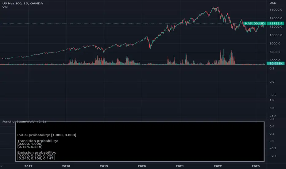
Library "FunctionBaumWelch"
Baum-Welch Algorithm, also known as Forward-Backward Algorithm, uses the well known EM algorithm
to find the maximum likelihood estimate of the parameters of a hidden Markov model given a set of observed
feature vectors.
---
### Function List:
> `forward (array<float> pi, matrix<float> a, matrix<float> b, array<int> obs)`
> `forward (array<float> pi, matrix<float> a, matrix<float> b, array<int> obs, bool scaling)`
> `backward (matrix<float> a, matrix<float> b, array<int> obs)`
> `backward (matrix<float> a, matrix<float> b, array<int> obs, array<float> c)`
> `baumwelch (array<int> observations, int nstates)`
> `baumwelch (array<int> observations, array<float> pi, matrix<float> a, matrix<float> b)`
---
### Reference:
> en.wikipedia.org/wiki/Baum–Welch_algorithm
> github.com/alexsosn/MarslandMLAlgo/blob/4277b24db88c4cb70d6b249921c5d21bc8f86eb4/Ch16/HMM.py
> en.wikipedia.org/wiki/Forward_algorithm
> rdocumentation.org/packages/HMM/versions/1.0.1/topics/forward
> rdocumentation.org/packages/HMM/versions/1.0.1/topics/backward
forward(pi, a, b, obs)
Computes forward probabilities for state `X` up to observation at time `k`, is defined as the
probability of observing sequence of observations `e_1 ... e_k` and that the state at time `k` is `X`.
Parameters:
pi (float[]): Initial probabilities.
a (matrix<float>): Transmissions, hidden transition matrix a or alpha = transition probability matrix of changing
states given a state matrix is size (M x M) where M is number of states.
b (matrix<float>): Emissions, matrix of observation probabilities b or beta = observation probabilities. Given
state matrix is size (M x O) where M is number of states and O is number of different
possible observations.
obs (int[]): List with actual state observation data.
Returns: - `matrix<float> _alpha`: Forward probabilities. The probabilities are given on a logarithmic scale (natural logarithm). The first
dimension refers to the state and the second dimension to time.
forward(pi, a, b, obs, scaling)
Computes forward probabilities for state `X` up to observation at time `k`, is defined as the
probability of observing sequence of observations `e_1 ... e_k` and that the state at time `k` is `X`.
Parameters:
pi (float[]): Initial probabilities.
a (matrix<float>): Transmissions, hidden transition matrix a or alpha = transition probability matrix of changing
states given a state matrix is size (M x M) where M is number of states.
b (matrix<float>): Emissions, matrix of observation probabilities b or beta = observation probabilities. Given
state matrix is size (M x O) where M is number of states and O is number of different
possible observations.
obs (int[]): List with actual state observation data.
scaling (bool): Normalize `alpha` scale.
Returns: - #### Tuple with:
> - `matrix<float> _alpha`: Forward probabilities. The probabilities are given on a logarithmic scale (natural logarithm). The first
dimension refers to the state and the second dimension to time.
> - `array<float> _c`: Array with normalization scale.
backward(a, b, obs)
Computes backward probabilities for state `X` and observation at time `k`, is defined as the probability of observing the sequence of observations `e_k+1, ... , e_n` under the condition that the state at time `k` is `X`.
Parameters:
a (matrix<float>): Transmissions, hidden transition matrix a or alpha = transition probability matrix of changing states
given a state matrix is size (M x M) where M is number of states
b (matrix<float>): Emissions, matrix of observation probabilities b or beta = observation probabilities. given state
matrix is size (M x O) where M is number of states and O is number of different possible observations
obs (int[]): Array with actual state observation data.
Returns: - `matrix<float> _beta`: Backward probabilities. The probabilities are given on a logarithmic scale (natural logarithm). The first dimension refers to the state and the second dimension to time.
backward(a, b, obs, c)
Computes backward probabilities for state `X` and observation at time `k`, is defined as the probability of observing the sequence of observations `e_k+1, ... , e_n` under the condition that the state at time `k` is `X`.
Parameters:
a (matrix<float>): Transmissions, hidden transition matrix a or alpha = transition probability matrix of changing states
given a state matrix is size (M x M) where M is number of states
b (matrix<float>): Emissions, matrix of observation probabilities b or beta = observation probabilities. given state
matrix is size (M x O) where M is number of states and O is number of different possible observations
obs (int[]): Array with actual state observation data.
c (float[]): Array with Normalization scaling coefficients.
Returns: - `matrix<float> _beta`: Backward probabilities. The probabilities are given on a logarithmic scale (natural logarithm). The first dimension refers to the state and the second dimension to time.
baumwelch(observations, nstates)
**(Random Initialization)** Baum–Welch algorithm is a special case of the expectation–maximization algorithm used to find the
unknown parameters of a hidden Markov model (HMM). It makes use of the forward-backward algorithm
to compute the statistics for the expectation step.
Parameters:
observations (int[]): List of observed states.
nstates (int)
Returns: - #### Tuple with:
> - `array<float> _pi`: Initial probability distribution.
> - `matrix<float> _a`: Transition probability matrix.
> - `matrix<float> _b`: Emission probability matrix.
---
requires: `import RicardoSantos/WIPTensor/2 as Tensor`
baumwelch(observations, pi, a, b)
Baum–Welch algorithm is a special case of the expectation–maximization algorithm used to find the
unknown parameters of a hidden Markov model (HMM). It makes use of the forward-backward algorithm
to compute the statistics for the expectation step.
Parameters:
observations (int[]): List of observed states.
pi (float[]): Initial probaility distribution.
a (matrix<float>): Transmissions, hidden transition matrix a or alpha = transition probability matrix of changing states
given a state matrix is size (M x M) where M is number of states
b (matrix<float>): Emissions, matrix of observation probabilities b or beta = observation probabilities. given state
matrix is size (M x O) where M is number of states and O is number of different possible observations
Returns: - #### Tuple with:
> - `array<float> _pi`: Initial probability distribution.
> - `matrix<float> _a`: Transition probability matrix.
> - `matrix<float> _b`: Emission probability matrix.
---
requires: `import RicardoSantos/WIPTensor/2 as Tensor`
發行說明
v2 minor update.發行說明
Fix logger version.發行說明
v4 - Added error checking for some errors.發行說明
v5 - Improved calculation by merging some of the loops, where possible.Pine腳本庫
秉持TradingView一貫精神,作者已將此Pine代碼以開源函式庫形式發佈,方便我們社群中的其他Pine程式設計師重複使用。向作者致敬!您可以在私人專案或其他開源發表中使用此函式庫,但在公開發表中重用此代碼須遵守社群規範。
免責聲明
這些資訊和出版物並非旨在提供,也不構成TradingView提供或認可的任何形式的財務、投資、交易或其他類型的建議或推薦。請閱讀使用條款以了解更多資訊。
Pine腳本庫
秉持TradingView一貫精神,作者已將此Pine代碼以開源函式庫形式發佈,方便我們社群中的其他Pine程式設計師重複使用。向作者致敬!您可以在私人專案或其他開源發表中使用此函式庫,但在公開發表中重用此代碼須遵守社群規範。
免責聲明
這些資訊和出版物並非旨在提供,也不構成TradingView提供或認可的任何形式的財務、投資、交易或其他類型的建議或推薦。請閱讀使用條款以了解更多資訊。