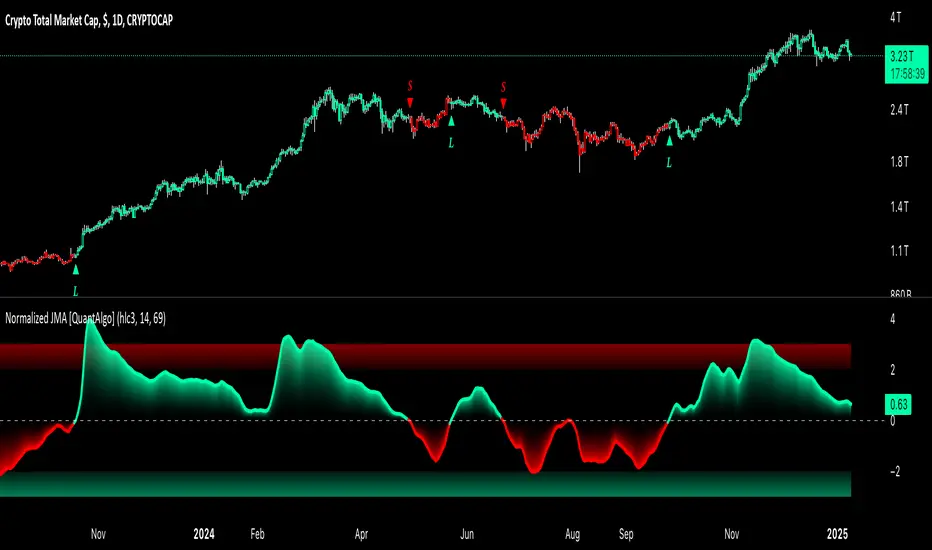
Normalized Jurik Moving Average [QuantAlgo]Upgrade your investing and trading strategy with the Normalized Jurik Moving Average (JMA) , a sophisticated oscillator that combines adaptive smoothing with statistical normalization to deliver high-quality signals! Whether you're a swing trader looking for momentum shifts or a medium- to long-term investor focusing on trend validation, this indicator's statistical approach offers valuable analytical advantages that can enhance your trading and investing decisions!
🟢 Core Architecture
The foundation of this indicator lies in its unique dual-layer calculation system. The first layer implements the Jurik Moving Average, known for its superior noise reduction and responsiveness, while the second layer applies statistical normalization (Z-Score) to create standardized readings. This sophisticated approach helps identify significant price movements while filtering out market noise across various timeframes and instruments.
🟢 Technical Foundation
Three key components power this indicator are:
Jurik Moving Average (JMA): An advanced moving average calculation that provides superior smoothing with minimal lag
Statistical Normalization: Z-Score based scaling that creates consistent, comparable readings across different market conditions
Dynamic Zone Detection: Automatically identifies overbought and oversold conditions based on statistical deviations
🟢 Key Features & Signals
The Normalized JMA delivers market insights through:
Color-adaptive oscillator line that reflects momentum strength and direction
Statistically significant overbought/oversold zones for trade validation
Smart gradient fills between signal line and zero level for enhanced visualization
Clear long (L) and short (S) markers for validated momentum shifts
Intelligent bar coloring that highlights the current market state
Customizable alert system for both bullish and bearish setups
🟢 Practical Usage Tips
Here's how to maximize your use of the Normalized JMA:
1/ Setup:
Add the indicator to your favorites, then apply it to your chart ⭐️
Begin with the default smoothing period for balanced analysis
Use the default normalization period for optimal signal generation
Start with standard visualization settings
Customize colors to match your chart preferences
Enable both bar coloring and signal markers for complete visual feedback
2/ Reading Signals:
Watch for L/S markers - they indicate validated momentum shifts
Monitor oscillator line color changes for direction confirmation
Use the built-in alert system to stay informed of potential trend changes
🟢 Pro Tips
Adjust Smoothing Period based on your trading style:
→ Lower values (8-12) for more responsive signals
→ Higher values (20-30) for more stable trend identification
Fine-tune Normalization Period based on market conditions:
→ Shorter periods (20-25) for more dynamic markets
→ Longer periods (40-50) for more stable markets
Optimize your analysis by:
→ Using +2/-2 zones for primary trade signals
→ Using +3/-3 zones for extreme market conditions
→ Combining with volume analysis for trade confirmation
→ Using multiple timeframe analysis for strategic context
Combine with:
→ Volume indicators for trade validation
→ Price action for entry timing
→ Support/resistance levels for profit targets
→ Trend-following indicators for directional bias
JMA
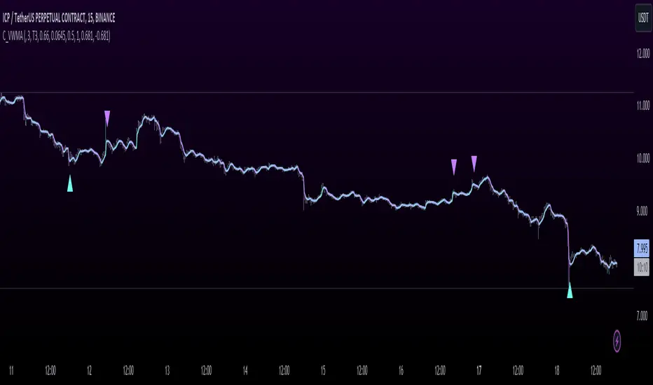
T3 JMA KAMA VWMAEnhancing Trading Performance with T3 JMA KAMA VWMA Indicator
Introduction
In the dynamic world of trading, staying ahead of market trends and capitalizing on volume-driven opportunities can greatly influence trading performance. To address this, we have developed the T3 JMA KAMA VWMA Indicator, an innovative tool that modifies the traditional Volume Weighted Moving Average (VWMA) formula to increase responsiveness and exploit high-volume market conditions for optimal position entry. This article delves into the idea behind this modification and how it can benefit traders seeking to gain an edge in the market.
The Idea Behind the Modification
The core concept behind modifying the VWMA formula is to leverage more responsive moving averages (MAs) that align with high-volume market activity. Traditional VWMA utilizes the Simple Moving Average (SMA) as the basis for calculating the weighted average. While the SMA is effective in providing a smoothed perspective of price movements, it may lack the desired responsiveness to capitalize on short-term volume-driven opportunities.
To address this limitation, our T3 JMA KAMA VWMA Indicator incorporates three advanced moving averages: T3, JMA, and KAMA. These MAs offer enhanced responsiveness, allowing traders to react swiftly to changing market conditions influenced by volume.
T3 (T3 New and T3 Normal):
The T3 moving average, one of the components of our indicator, applies a proprietary algorithm that provides smoother and more responsive trend signals. By utilizing T3, we ensure that the VWMA calculation aligns with the dynamic nature of high-volume markets, enabling traders to capture price movements accurately.
JMA (Jurik Moving Average):
The JMA component further enhances the indicator's responsiveness by incorporating phase shifting and power adjustment. This adaptive approach ensures that the moving average remains sensitive to changes in volume and price dynamics. As a result, traders can identify turning points and anticipate potential trend reversals, precisely timing their position entries.
KAMA (Kaufman's Adaptive Moving Average):
KAMA is an adaptive moving average designed to dynamically adjust its sensitivity based on market conditions. By incorporating KAMA into our VWMA modification, we ensure that the moving average adapts to varying volume levels and captures the essence of volume-driven price movements. Traders can confidently enter positions during periods of high trading volume, aligning their strategies with market activity.
Benefits and Usage
The modified T3 JMA KAMA VWMA Indicator offers several advantages to traders looking to exploit high-volume market conditions for position entry:
Increased Responsiveness: By incorporating more responsive moving averages, the indicator enables traders to react quickly to changes in volume and capture short-term opportunities more effectively.
Enhanced Entry Timing: The modified VWMA aligns with high-volume periods, allowing traders to enter positions precisely during price movements influenced by significant trading activity.
Improved Accuracy: The combination of T3, JMA, and KAMA within the VWMA formula enhances the accuracy of trend identification, reversals, and overall market analysis.
Comprehensive Market Insights: The T3 JMA KAMA VWMA Indicator provides a holistic view of market conditions by considering both price and volume dynamics. This comprehensive perspective helps traders make informed decisions.
Analysis and Interpretation
The modified VWMA formula with T3, JMA, and KAMA offers traders a valuable tool for analyzing volume-driven market conditions. By incorporating these advanced moving averages into the VWMA calculation, the indicator becomes more responsive to changes in volume, potentially providing deeper insights into price movements.
When analyzing the modified VWMA, it is essential to consider the following points:
Identifying High-Volume Periods:
The modified VWMA is designed to capture price movements during high-volume periods. Traders can use this indicator to identify potential market trends and determine whether significant trading activity is driving price action. By focusing on these periods, traders may gain a better understanding of the market sentiment and adjust their strategies accordingly.
Confirmation of Trend Strength:
The modified VWMA can serve as a confirmation tool for assessing the strength of a trend. When the VWMA line aligns with the overall trend direction, it suggests that the current price movement is supported by volume. This confirmation can provide traders with additional confidence in their analysis and help them make more informed trading decisions.
Potential Entry and Exit Points:
One of the primary purposes of the modified VWMA is to assist traders in identifying potential entry and exit points. By capturing volume-driven price movements, the indicator can highlight areas where market participants are actively participating, indicating potential opportunities for opening or closing positions. Traders can use this information in conjunction with other technical analysis tools to develop comprehensive trading strategies.
Interpretation of Angle and Gradient:
The modified VWMA incorporates an angle calculation and color gradient to further enhance interpretation. The angle of the VWMA line represents the slope of the indicator, providing insights into the momentum of price movements. A steep angle indicates strong momentum, while a shallow angle suggests a slowdown. The color gradient helps visualize this angle, with green indicating bullish momentum and purple indicating bearish momentum.
Conclusion
By modifying the VWMA formula to incorporate the T3, JMA, and KAMA moving averages, the T3 JMA KAMA VWMA Indicator offers traders an innovative tool to exploit high-volume market conditions for optimal position entry. This modification enhances responsiveness, improves timing, and provides comprehensive market insights.
Enjoy checking it out!
---
Credits to:
◾ @cheatcountry – Hann Window Smoothing
◾ @loxx – T3
◾ @everget – JMA
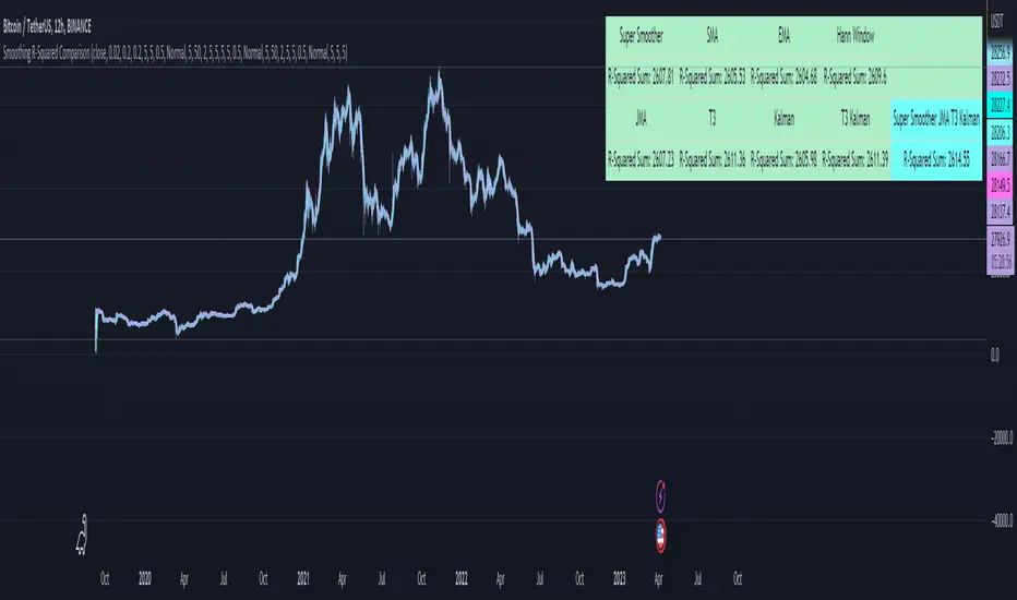
Smoothing R-Squared ComparisonIntroduction
Heyo guys, here I made a comparison between my favorised smoothing algorithms.
I chose the R-Squared value as rating factor to accomplish the comparison.
The indicator is non-repainting.
Description
In technical analysis, traders often use moving averages to smooth out the noise in price data and identify trends. While moving averages are a useful tool, they can also obscure important information about the underlying relationship between the price and the smoothed price.
One way to evaluate this relationship is by calculating the R-squared value, which represents the proportion of the variance in the price that can be explained by the smoothed price in a linear regression model.
This PineScript code implements a smoothing R-squared comparison indicator.
It provides a comparison of different smoothing techniques such as Kalman filter, T3, JMA, EMA, SMA, Super Smoother and some special combinations of them.
The Kalman filter is a mathematical algorithm that uses a series of measurements observed over time, containing statistical noise and other inaccuracies, and produces estimates of unknown variables that tend to be more accurate than those based on a single measurement.
The input parameters for the Kalman filter include the process noise covariance and the measurement noise covariance, which help to adjust the sensitivity of the filter to changes in the input data.
The T3 smoothing technique is a popular method used in technical analysis to remove noise from a signal.
The input parameters for the T3 smoothing method include the length of the window used for smoothing, the type of smoothing used (Normal or New), and the smoothing factor used to adjust the sensitivity to changes in the input data.
The JMA smoothing technique is another popular method used in technical analysis to remove noise from a signal.
The input parameters for the JMA smoothing method include the length of the window used for smoothing, the phase used to shift the input data before applying the smoothing algorithm, and the power used to adjust the sensitivity of the JMA to changes in the input data.
The EMA and SMA techniques are also popular methods used in technical analysis to remove noise from a signal.
The input parameters for the EMA and SMA techniques include the length of the window used for smoothing.
The indicator displays a comparison of the R-squared values for each smoothing technique, which provides an indication of how well the technique is fitting the data.
Higher R-squared values indicate a better fit. By adjusting the input parameters for each smoothing technique, the user can compare the effectiveness of different techniques in removing noise from the input data.
Usage
You can use it to find the best fitting smoothing method for the timeframe you usually use.
Just apply it on your preferred timeframe and look for the highlighted table cell.
Conclusion
It seems like the T3 works best on timeframes under 4H.
There's where I am active, so I will use this one more in the future.
Thank you for checking this out. Enjoy your day and leave me a like or comment. 🧙♂️
---
Credits to:
▪@loxx – T3
▪@balipour – Super Smoother
▪ChatGPT – Wrote 80 % of this article and helped with the research
Softmax Normalized Jurik Filter Histogram [Loxx]Softmax Normalized Jurik Filter Histogram is a Jurik Filter that is morphed into a normalized oscillator from -1 to 1.
What is the Softmax function?
The softmax function, also known as softargmax: or normalized exponential function, converts a vector of K real numbers into a probability distribution of K possible outcomes. It is a generalization of the logistic function to multiple dimensions, and used in multinomial logistic regression. The softmax function is often used as the last activation function of a neural network to normalize the output of a network to a probability distribution over predicted output classes, based on Luce's choice axiom.
What is Jurik Volty used in the Juirk Filter?
One of the lesser known qualities of Juirk smoothing is that the Jurik smoothing process is adaptive. "Jurik Volty" (a sort of market volatility ) is what makes Jurik smoothing adaptive. The Jurik Volty calculation can be used as both a standalone indicator and to smooth other indicators that you wish to make adaptive.
What is the Jurik Moving Average?
Have you noticed how moving averages add some lag (delay) to your signals? ... especially when price gaps up or down in a big move, and you are waiting for your moving average to catch up? Wait no more! JMA eliminates this problem forever and gives you the best of both worlds: low lag and smooth lines.
Included:
Bar coloring
Signals
Alerts
Loxx's Expanded Source Types

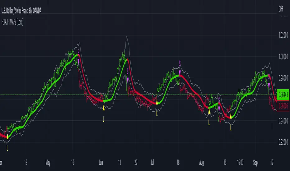
FDI-Adaptive, Jurik-Filtered, TMA w/ Price Zones [Loxx]FDI-Adaptive, Jurik-Filtered, TMA w/ Price Zones is a Triangular Moving Average that is Fractal Dimension Index Adaptive with Jurik Smoothing. You'll notice that this combination not only smooths out the signal but also catches bottoms better than other FIR digital filters. This is a multi-layered adaptive moving average. Price zones are calculated using a weighted range function. Future updates will included signals associated with these range bands. For now, however, these range bands serve as support and resistance, stop-loss or take profit, or indicators of market reversal.
What is the Triangular Moving Average
The Triangular Moving Average is basically a double-smoothed Simple Moving Average that gives more weight to the middle section of the data interval. The TMA has a significant lag to current prices and is not well-suited to fast moving markets. TMA = SUM ( SMA values)/ N Where N = the number of periods.
What is the Fractal Dimension Index?
The goal of the fractal dimension index is to determine whether the market is trending or in a trading range. It does not measure the direction of the trend. A value less than 1.5 indicates that the price series is persistent or that the market is trending. Lower values of the FDI indicate a stronger trend. A value greater than 1.5 indicates that the market is in a trading range and is acting in a more random fashion.
What is Jurik Volty used in the Juirk Filter?
One of the lesser known qualities of Juirk smoothing is that the Jurik smoothing process is adaptive. "Jurik Volty" (a sort of market volatility ) is what makes Jurik smoothing adaptive. The Jurik Volty calculation can be used as both a standalone indicator and to smooth other indicators that you wish to make adaptive.
What is the Jurik Moving Average?
Have you noticed how moving averages add some lag (delay) to your signals? ... especially when price gaps up or down in a big move, and you are waiting for your moving average to catch up? Wait no more! JMA eliminates this problem forever and gives you the best of both worlds: low lag and smooth lines.
Included:
Bar coloring
Signals
Alerts
Jurik-Filtered Kase Permission Stochastic [Loxx]Jurik-Filtered Kase Permission Stochastic is a special implementation of Kase Permission Stochastic by Kase StatWare. This implementation uses a Jurik filter to smooth final output.
What is Kase StatWare?
Kase StatWare has been around since 1992 and is a technical analysis trading indicator package developed by the acclaimed market technician and former energy trader Cynthia A. Kase. StatWare’s self-optimizing indicators help professional and individual traders to form a precise and systematic approach to discretionary trading and trade risk management.
Kase StatWare creates subscription-based technical analysis tools mainly for Stocks and Futures trading which can be subscribed to at a monthly cost.
What is Kase Permission Stochastic?
The Kase Permission Stochastic is a momentum indicator that examines a synthetic longer bar length, that by default, is three (5x by default for this implementation here) times higher than the bar length it is plotted against.
Included
Alerts
Signals
Bar coloring
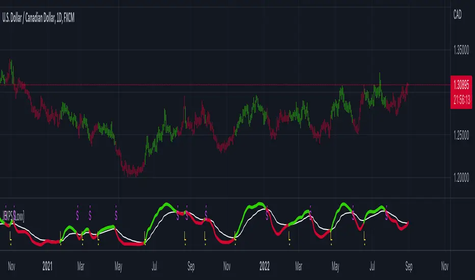
CFB-Adaptive, Jurik DMX Histogram [Loxx]Jurik DMX Histogram is the ultra-smooth, low lag version of your classic DMI indicator. This is a momentum indicator. You can use this indicator standalone or as part of a system with a moving average and a mean reversion indicator. This indicator has both composite fractal behavior adaptive inputs and fixed inputs. The default is CFB adaptive. Dark green means strong push up, dark red, strong push down. Light green means weak push up, and light red means weak push down.
What is the directional movement index?
The directional movement index (DMI) is an indicator developed by J. Welles Wilder in 1978 that identifies in which direction the price of an asset is moving. The indicator does this by comparing prior highs and lows and drawing two lines: a positive directional movement line ( +DI ) and a negative directional movement line ( -DI ). An optional third line, called the average directional index ( ADX ), can also be used to gauge the strength of the uptrend or downtrend.
When +DI is above -DI , there is more upward pressure than downward pressure in the price. Conversely, if -DI is above +DI , then there is more downward pressure on the price. This indicator may help traders assess the trend direction. Crossovers between the lines are also sometimes used as trade signals to buy or sell.
What is Composite Fractal Behavior ( CFB )?
All around you mechanisms adjust themselves to their environment. From simple thermostats that react to air temperature to computer chips in modern cars that respond to changes in engine temperature, r.p.m.'s, torque, and throttle position. It was only a matter of time before fast desktop computers applied the mathematics of self-adjustment to systems that trade the financial markets.
Unlike basic systems with fixed formulas, an adaptive system adjusts its own equations. For example, start with a basic channel breakout system that uses the highest closing price of the last N bars as a threshold for detecting breakouts on the up side. An adaptive and improved version of this system would adjust N according to market conditions, such as momentum, price volatility or acceleration.
Since many systems are based directly or indirectly on cycles, another useful measure of market condition is the periodic length of a price chart's dominant cycle, (DC), that cycle with the greatest influence on price action.
The utility of this new DC measure was noted by author Murray Ruggiero in the January '96 issue of Futures Magazine. In it. Mr. Ruggiero used it to adaptive adjust the value of N in a channel breakout system. He then simulated trading 15 years of D-Mark futures in order to compare its performance to a similar system that had a fixed optimal value of N. The adaptive version produced 20% more profit!
This DC index utilized the popular MESA algorithm (a formulation by John Ehlers adapted from Burg's maximum entropy algorithm, MEM). Unfortunately, the DC approach is problematic when the market has no real dominant cycle momentum, because the mathematics will produce a value whether or not one actually exists! Therefore, we developed a proprietary indicator that does not presuppose the presence of market cycles. It's called CFB (Composite Fractal Behavior) and it works well whether or not the market is cyclic.
CFB examines price action for a particular fractal pattern, categorizes them by size, and then outputs a composite fractal size index. This index is smooth, timely and accurate
Essentially, CFB reveals the length of the market's trending action time frame. Long trending activity produces a large CFB index and short choppy action produces a small index value. Investors have found many applications for CFB which involve scaling other existing technical indicators adaptively, on a bar-to-bar basis.
What is Jurik Volty used in the Juirk Filter?
One of the lesser known qualities of Juirk smoothing is that the Jurik smoothing process is adaptive. "Jurik Volty" (a sort of market volatility ) is what makes Jurik smoothing adaptive. The Jurik Volty calculation can be used as both a standalone indicator and to smooth other indicators that you wish to make adaptive.
What is the Jurik Moving Average?
Have you noticed how moving averages add some lag (delay) to your signals? ... especially when price gaps up or down in a big move, and you are waiting for your moving average to catch up? Wait no more! JMA eliminates this problem forever and gives you the best of both worlds: low lag and smooth lines.
Ideally, you would like a filtered signal to be both smooth and lag-free. Lag causes delays in your trades, and increasing lag in your indicators typically result in lower profits. In other words, late comers get what's left on the table after the feast has already begun.
Included:
Alerts
Loxx's Expanded Source Types
Signals
Bar coloring

Adaptive-Lookback CCI w/ Double Juirk Smoothing [Loxx]Adaptive-Lookback CCI w/ Double Juirk Smoothing is a CCI indicator with Adaptive period inputs. The adaptive calculation in this case is the count of pivots in historical bars. This indicator is also double smoothing using Jurik smoothing to reduce noise and refine the signal.
What is CCI?
The Commodity Channel Index ( CCI ) measures the current price level relative to an average price level over a given period of time. CCI is relatively high when prices are far above their average. CCI is relatively low when prices are far below their average. Using this method, CCI can be used to identify overbought and oversold levels.
What is Jurik Volty used in the Juirk Filter?
One of the lesser known qualities of Juirk smoothing is that the Jurik smoothing process is adaptive. "Jurik Volty" (a sort of market volatility ) is what makes Jurik smoothing adaptive. The Jurik Volty calculation can be used as both a standalone indicator and to smooth other indicators that you wish to make adaptive.
What is the Jurik Moving Average?
Have you noticed how moving averages add some lag (delay) to your signals? ... especially when price gaps up or down in a big move, and you are waiting for your moving average to catch up? Wait no more! JMA eliminates this problem forever and gives you the best of both worlds: low lag and smooth lines.
Included:
Bar coloring
3 signal variations w/ alerts

True Adaptive-Lookback Phase Change Index [Loxx]Previously I posted a Phase Change Index using Ehlers Autocorrelation Periodogram Algorithm to tease out the adaptive periods. You can find the previous version here: . This new version is also adaptive but uses a different method to derive the adaptive length inputs. This adaptive method derives period inputs by counting pivots from past candles. This version also relies on Jurik Smoothing to generate the final signal. I named this one "true" because I should have specified in the previous PCI's title that it's powered by Ehlers Autocorrelation Periodogram. Additionally, you'll notice the ALB algorithm has changed from other indicators, This is restrict the range of possible ALB period outputs to a specific range so the indicator is usable.
And remember, this is an inverse indicator. This means that small values on the oscillator indicate bullish sentiment and higher values on the oscillator indicate bearish sentiment.
What is the Phase Change Index?
Based on the M.H. Pee's TASC article "Phase Change Index".
Prices at any time can be up, down, or unchanged. A period where market prices remain relatively unchanged is referred to as a consolidation. A period that witnesses relatively higher prices is referred to as an uptrend, while a period of relatively lower prices is called a downtrend.
The Phase Change Index ( PCI ) is an indicator designed specifically to detect changes in market phases.
This indicator is made as he describes it with one deviation: if we follow his formula to the letter then the "trend" is inverted to the actual market trend. Because of that an option to display inverted (and more logical) values is added.
What is the Jurik Moving Average?
Have you noticed how moving averages add some lag (delay) to your signals? ... especially when price gaps up or down in a big move, and you are waiting for your moving average to catch up? Wait no more! JMA eliminates this problem forever and gives you the best of both worlds: low lag and smooth lines.
Ideally, you would like a filtered signal to be both smooth and lag-free. Lag causes delays in your trades, and increasing lag in your indicators typically result in lower profits. In other words, late comers get what's left on the table after the feast has already begun.
That's why investors, banks and institutions worldwide ask for the Jurik Research Moving Average ( JMA ). You may apply it just as you would any other popular moving average. However, JMA's improved timing and smoothness will astound you.
What is adaptive Jurik volatility
One of the lesser known qualities of Juirk smoothing is that the Jurik smoothing process is adaptive. "Jurik Volty" (a sort of market volatility ) is what makes Jurik smoothing adaptive. The Jurik Volty calculation can be used as both a standalone indicator and to smooth other indicators that you wish to make adaptive.
Included:
Bar coloring
2 signal variations w/ alerts

Adaptive-LB, Jurik-Filtered, Triangular MA w/ Price Zones [Loxx]Adaptive-LB, Jurik-Filtered, Triangular MA w/ Price Zones is a moving average indicator that takes as its input an adaptive lookback period. This is an experimental indicator and I wouldn't use this for trading. It's more to explore different adaptive calculation methods and their applications to moving averages and channels. Unlike the traditional Triangular Moving Average, this one uses Jurik smoothing.
What is the Triangular Moving Average
The Triangular Moving Average is basically a double-smoothed Simple Moving Average that gives more weight to the middle section of the data interval. The TMA has a significant lag to current prices and is not well-suited to fast moving markets. TMA = SUM (SMA values)/ N Where N = the number of periods.
What is Jurik Volty used in the Juirk Filter?
One of the lesser known qualities of Juirk smoothing is that the Jurik smoothing process is adaptive. "Jurik Volty" (a sort of market volatility ) is what makes Jurik smoothing adaptive. The Jurik Volty calculation can be used as both a standalone indicator and to smooth other indicators that you wish to make adaptive.
What is the Jurik Moving Average?
Have you noticed how moving averages add some lag (delay) to your signals? ... especially when price gaps up or down in a big move, and you are waiting for your moving average to catch up? Wait no more! JMA eliminates this problem forever and gives you the best of both worlds: low lag and smooth lines.
Included:
Bar coloring
Signals
Alerts

CFB-Adaptive Velocity Histogram [Loxx]CFB-Adaptive Velocity Histogram is a velocity indicator with One-More-Moving-Average Adaptive Smoothing of input source value and Jurik's Composite-Fractal-Behavior-Adaptive Price-Trend-Period input with Dynamic Zones. All Juirk smoothing allows for both single and double Jurik smoothing passes. Velocity is adjusted to pips but there is no input value for the user. This indicator is tuned for Forex but can be used on any time series data.
What is Composite Fractal Behavior ( CFB )?
All around you mechanisms adjust themselves to their environment. From simple thermostats that react to air temperature to computer chips in modern cars that respond to changes in engine temperature, r.p.m.'s, torque, and throttle position. It was only a matter of time before fast desktop computers applied the mathematics of self-adjustment to systems that trade the financial markets.
Unlike basic systems with fixed formulas, an adaptive system adjusts its own equations. For example, start with a basic channel breakout system that uses the highest closing price of the last N bars as a threshold for detecting breakouts on the up side. An adaptive and improved version of this system would adjust N according to market conditions, such as momentum, price volatility or acceleration.
Since many systems are based directly or indirectly on cycles, another useful measure of market condition is the periodic length of a price chart's dominant cycle, (DC), that cycle with the greatest influence on price action.
The utility of this new DC measure was noted by author Murray Ruggiero in the January '96 issue of Futures Magazine. In it. Mr. Ruggiero used it to adaptive adjust the value of N in a channel breakout system. He then simulated trading 15 years of D-Mark futures in order to compare its performance to a similar system that had a fixed optimal value of N. The adaptive version produced 20% more profit!
This DC index utilized the popular MESA algorithm (a formulation by John Ehlers adapted from Burg's maximum entropy algorithm, MEM). Unfortunately, the DC approach is problematic when the market has no real dominant cycle momentum, because the mathematics will produce a value whether or not one actually exists! Therefore, we developed a proprietary indicator that does not presuppose the presence of market cycles. It's called CFB (Composite Fractal Behavior) and it works well whether or not the market is cyclic.
CFB examines price action for a particular fractal pattern, categorizes them by size, and then outputs a composite fractal size index. This index is smooth, timely and accurate
Essentially, CFB reveals the length of the market's trending action time frame. Long trending activity produces a large CFB index and short choppy action produces a small index value. Investors have found many applications for CFB which involve scaling other existing technical indicators adaptively, on a bar-to-bar basis.
What is Jurik Volty used in the Juirk Filter?
One of the lesser known qualities of Juirk smoothing is that the Jurik smoothing process is adaptive. "Jurik Volty" (a sort of market volatility ) is what makes Jurik smoothing adaptive. The Jurik Volty calculation can be used as both a standalone indicator and to smooth other indicators that you wish to make adaptive.
What is the Jurik Moving Average?
Have you noticed how moving averages add some lag (delay) to your signals? ... especially when price gaps up or down in a big move, and you are waiting for your moving average to catch up? Wait no more! JMA eliminates this problem forever and gives you the best of both worlds: low lag and smooth lines.
Ideally, you would like a filtered signal to be both smooth and lag-free. Lag causes delays in your trades, and increasing lag in your indicators typically result in lower profits. In other words, late comers get what's left on the table after the feast has already begun.
What are Dynamic Zones?
As explained in "Stocks & Commodities V15:7 (306-310): Dynamic Zones by Leo Zamansky, Ph .D., and David Stendahl"
Most indicators use a fixed zone for buy and sell signals. Here’ s a concept based on zones that are responsive to past levels of the indicator.
One approach to active investing employs the use of oscillators to exploit tradable market trends. This investing style follows a very simple form of logic: Enter the market only when an oscillator has moved far above or below traditional trading lev- els. However, these oscillator- driven systems lack the ability to evolve with the market because they use fixed buy and sell zones. Traders typically use one set of buy and sell zones for a bull market and substantially different zones for a bear market. And therein lies the problem.
Once traders begin introducing their market opinions into trading equations, by changing the zones, they negate the system’s mechanical nature. The objective is to have a system automatically define its own buy and sell zones and thereby profitably trade in any market — bull or bear. Dynamic zones offer a solution to the problem of fixed buy and sell zones for any oscillator-driven system.
An indicator’s extreme levels can be quantified using statistical methods. These extreme levels are calculated for a certain period and serve as the buy and sell zones for a trading system. The repetition of this statistical process for every value of the indicator creates values that become the dynamic zones. The zones are calculated in such a way that the probability of the indicator value rising above, or falling below, the dynamic zones is equal to a given probability input set by the trader.
To better understand dynamic zones, let's first describe them mathematically and then explain their use. The dynamic zones definition:
Find V such that:
For dynamic zone buy: P{X <= V}=P1
For dynamic zone sell: P{X >= V}=P2
where P1 and P2 are the probabilities set by the trader, X is the value of the indicator for the selected period and V represents the value of the dynamic zone.
The probability input P1 and P2 can be adjusted by the trader to encompass as much or as little data as the trader would like. The smaller the probability, the fewer data values above and below the dynamic zones. This translates into a wider range between the buy and sell zones. If a 10% probability is used for P1 and P2, only those data values that make up the top 10% and bottom 10% for an indicator are used in the construction of the zones. Of the values, 80% will fall between the two extreme levels. Because dynamic zone levels are penetrated so infrequently, when this happens, traders know that the market has truly moved into overbought or oversold territory.
Calculating the Dynamic Zones
The algorithm for the dynamic zones is a series of steps. First, decide the value of the lookback period t. Next, decide the value of the probability Pbuy for buy zone and value of the probability Psell for the sell zone.
For i=1, to the last lookback period, build the distribution f(x) of the price during the lookback period i. Then find the value Vi1 such that the probability of the price less than or equal to Vi1 during the lookback period i is equal to Pbuy. Find the value Vi2 such that the probability of the price greater or equal to Vi2 during the lookback period i is equal to Psell. The sequence of Vi1 for all periods gives the buy zone. The sequence of Vi2 for all periods gives the sell zone.
In the algorithm description, we have: Build the distribution f(x) of the price during the lookback period i. The distribution here is empirical namely, how many times a given value of x appeared during the lookback period. The problem is to find such x that the probability of a price being greater or equal to x will be equal to a probability selected by the user. Probability is the area under the distribution curve. The task is to find such value of x that the area under the distribution curve to the right of x will be equal to the probability selected by the user. That x is the dynamic zone.
Included:
Bar coloring
3 signal variations w/ alerts
Divergences w/ alerts
Loxx's Expanded Source Types
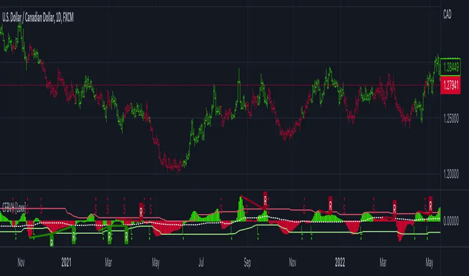
CFB-Adaptive, Williams %R w/ Dynamic Zones [Loxx]CFB-Adaptive, Williams %R w/ Dynamic Zones is a Jurik-Composite-Fractal-Behavior-Adaptive Williams % Range indicator with Dynamic Zones. These additions to the WPR calculation reduce noise and return a signal that is more viable than WPR alone.
What is Williams %R?
Williams %R , also known as the Williams Percent Range, is a type of momentum indicator that moves between 0 and -100 and measures overbought and oversold levels. The Williams %R may be used to find entry and exit points in the market. The indicator is very similar to the Stochastic oscillator and is used in the same way. It was developed by Larry Williams and it compares a stock’s closing price to the high-low range over a specific period, typically 14 days or periods.
What is Composite Fractal Behavior ( CFB )?
All around you mechanisms adjust themselves to their environment. From simple thermostats that react to air temperature to computer chips in modern cars that respond to changes in engine temperature, r.p.m.'s, torque, and throttle position. It was only a matter of time before fast desktop computers applied the mathematics of self-adjustment to systems that trade the financial markets.
Unlike basic systems with fixed formulas, an adaptive system adjusts its own equations. For example, start with a basic channel breakout system that uses the highest closing price of the last N bars as a threshold for detecting breakouts on the up side. An adaptive and improved version of this system would adjust N according to market conditions, such as momentum, price volatility or acceleration.
Since many systems are based directly or indirectly on cycles, another useful measure of market condition is the periodic length of a price chart's dominant cycle, (DC), that cycle with the greatest influence on price action.
The utility of this new DC measure was noted by author Murray Ruggiero in the January '96 issue of Futures Magazine. In it. Mr. Ruggiero used it to adaptive adjust the value of N in a channel breakout system. He then simulated trading 15 years of D-Mark futures in order to compare its performance to a similar system that had a fixed optimal value of N. The adaptive version produced 20% more profit!
This DC index utilized the popular MESA algorithm (a formulation by John Ehlers adapted from Burg's maximum entropy algorithm, MEM). Unfortunately, the DC approach is problematic when the market has no real dominant cycle momentum, because the mathematics will produce a value whether or not one actually exists! Therefore, we developed a proprietary indicator that does not presuppose the presence of market cycles. It's called CFB (Composite Fractal Behavior) and it works well whether or not the market is cyclic.
CFB examines price action for a particular fractal pattern, categorizes them by size, and then outputs a composite fractal size index. This index is smooth, timely and accurate
Essentially, CFB reveals the length of the market's trending action time frame. Long trending activity produces a large CFB index and short choppy action produces a small index value. Investors have found many applications for CFB which involve scaling other existing technical indicators adaptively, on a bar-to-bar basis.
What is Jurik Volty used in the Juirk Filter?
One of the lesser known qualities of Juirk smoothing is that the Jurik smoothing process is adaptive. "Jurik Volty" (a sort of market volatility ) is what makes Jurik smoothing adaptive. The Jurik Volty calculation can be used as both a standalone indicator and to smooth other indicators that you wish to make adaptive.
What is the Jurik Moving Average?
Have you noticed how moving averages add some lag (delay) to your signals? ... especially when price gaps up or down in a big move, and you are waiting for your moving average to catch up? Wait no more! JMA eliminates this problem forever and gives you the best of both worlds: low lag and smooth lines.
Ideally, you would like a filtered signal to be both smooth and lag-free. Lag causes delays in your trades, and increasing lag in your indicators typically result in lower profits. In other words, late comers get what's left on the table after the feast has already begun.
What are Dynamic Zones?
As explained in "Stocks & Commodities V15:7 (306-310): Dynamic Zones by Leo Zamansky, Ph .D., and David Stendahl"
Most indicators use a fixed zone for buy and sell signals. Here’ s a concept based on zones that are responsive to past levels of the indicator.
One approach to active investing employs the use of oscillators to exploit tradable market trends. This investing style follows a very simple form of logic: Enter the market only when an oscillator has moved far above or below traditional trading lev- els. However, these oscillator- driven systems lack the ability to evolve with the market because they use fixed buy and sell zones. Traders typically use one set of buy and sell zones for a bull market and substantially different zones for a bear market. And therein lies the problem.
Once traders begin introducing their market opinions into trading equations, by changing the zones, they negate the system’s mechanical nature. The objective is to have a system automatically define its own buy and sell zones and thereby profitably trade in any market — bull or bear. Dynamic zones offer a solution to the problem of fixed buy and sell zones for any oscillator-driven system.
An indicator’s extreme levels can be quantified using statistical methods. These extreme levels are calculated for a certain period and serve as the buy and sell zones for a trading system. The repetition of this statistical process for every value of the indicator creates values that become the dynamic zones. The zones are calculated in such a way that the probability of the indicator value rising above, or falling below, the dynamic zones is equal to a given probability input set by the trader.
To better understand dynamic zones, let's first describe them mathematically and then explain their use. The dynamic zones definition:
Find V such that:
For dynamic zone buy: P{X <= V}=P1
For dynamic zone sell: P{X >= V}=P2
where P1 and P2 are the probabilities set by the trader, X is the value of the indicator for the selected period and V represents the value of the dynamic zone.
The probability input P1 and P2 can be adjusted by the trader to encompass as much or as little data as the trader would like. The smaller the probability, the fewer data values above and below the dynamic zones. This translates into a wider range between the buy and sell zones. If a 10% probability is used for P1 and P2, only those data values that make up the top 10% and bottom 10% for an indicator are used in the construction of the zones. Of the values, 80% will fall between the two extreme levels. Because dynamic zone levels are penetrated so infrequently, when this happens, traders know that the market has truly moved into overbought or oversold territory.
Calculating the Dynamic Zones
The algorithm for the dynamic zones is a series of steps. First, decide the value of the lookback period t. Next, decide the value of the probability Pbuy for buy zone and value of the probability Psell for the sell zone.
For i=1, to the last lookback period, build the distribution f(x) of the price during the lookback period i. Then find the value Vi1 such that the probability of the price less than or equal to Vi1 during the lookback period i is equal to Pbuy. Find the value Vi2 such that the probability of the price greater or equal to Vi2 during the lookback period i is equal to Psell. The sequence of Vi1 for all periods gives the buy zone. The sequence of Vi2 for all periods gives the sell zone.
In the algorithm description, we have: Build the distribution f(x) of the price during the lookback period i. The distribution here is empirical namely, how many times a given value of x appeared during the lookback period. The problem is to find such x that the probability of a price being greater or equal to x will be equal to a probability selected by the user. Probability is the area under the distribution curve. The task is to find such value of x that the area under the distribution curve to the right of x will be equal to the probability selected by the user. That x is the dynamic zone.
Included:
Bar coloring
3 signal variations w/ alerts
Divergences w/ alerts
Loxx's Expanded Source Types

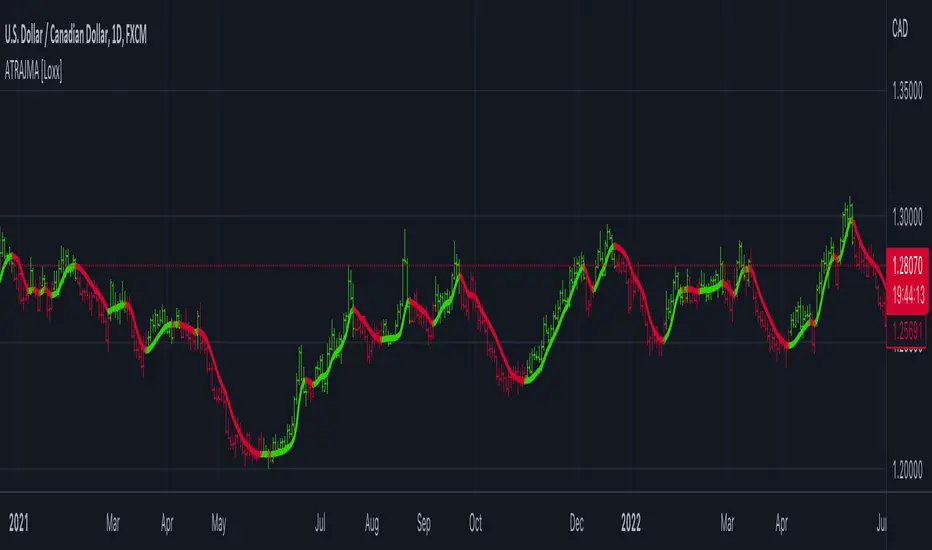
ATR-Adaptive JMA [Loxx]Not many know that the JMA (Jurik Moving Average) is already an adaptive indicator (it is adapting using the usual market volatility monitoring mode). Hence, making it adaptive "once more" makes it double adaptive. Fro the adaptivity in this case, we are use ATR (Average True Range) to make the JMA double adaptive. The ATR period is the same as the JMA period (there is no separate setting for that) so the usage of the indicator is as simple as it gets.
What is Jurik Volty used in the Juirk Filter?
One of the lesser known qualities of Juirk smoothing is that the Jurik smoothing process is adaptive. "Jurik Volty" (a sort of market volatility ) is what makes Jurik smoothing adaptive. The Jurik Volty calculation can be used as both a standalone indicator and to smooth other indicators that you wish to make adaptive.
What is the Jurik Moving Average?
Have you noticed how moving averages add some lag (delay) to your signals? ... especially when price gaps up or down in a big move, and you are waiting for your moving average to catch up? Wait no more! JMA eliminates this problem forever and gives you the best of both worlds: low lag and smooth lines.
Included:
Bar coloring
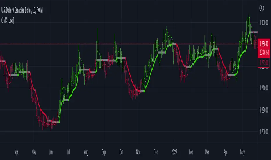
Corrected JMA [Loxx]This indicator uses the Juirk Moving Average to calculate price deviations from the JMA and if the changes are not significant, then the value is "flattened". That way we can easily see both trends and potential chop zones. This uses the regular JMA as a trigger.
What is Jurik Volty used in the Juirk Filter?
One of the lesser known qualities of Juirk smoothing is that the Jurik smoothing process is adaptive. "Jurik Volty" (a sort of market volatility ) is what makes Jurik smoothing adaptive. The Jurik Volty calculation can be used as both a standalone indicator and to smooth other indicators that you wish to make adaptive.
What is the Jurik Moving Average?
Have you noticed how moving averages add some lag (delay) to your signals? ... especially when price gaps up or down in a big move, and you are waiting for your moving average to catch up? Wait no more! JMA eliminates this problem forever and gives you the best of both worlds: low lag and smooth lines.
Included:
Bar coloring
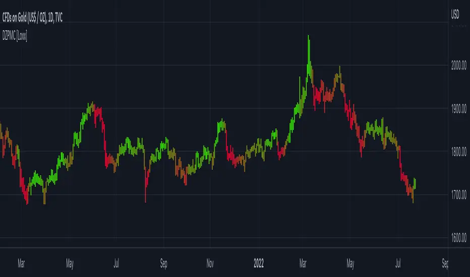
Dynamic Zones Polychromatic Momentum Candles [Loxx]Dynamic Zones Polychromatic Momentum Candles is a candle coloring, momentum indicator that uses Jurik Filtering and Dynamic Zones to calculate the monochromatic color between two colors.
What is Jurik Volty used in the Juirk Filter?
One of the lesser known qualities of Juirk smoothing is that the Jurik smoothing process is adaptive. "Jurik Volty" (a sort of market volatility ) is what makes Jurik smoothing adaptive. The Jurik Volty calculation can be used as both a standalone indicator and to smooth other indicators that you wish to make adaptive.
What is the Jurik Moving Average?
Have you noticed how moving averages add some lag (delay) to your signals? ... especially when price gaps up or down in a big move, and you are waiting for your moving average to catch up? Wait no more! JMA eliminates this problem forever and gives you the best of both worlds: low lag and smooth lines.
What are Dynamic Zones?
As explained in "Stocks & Commodities V15:7 (306-310): Dynamic Zones by Leo Zamansky, Ph .D., and David Stendahl"
Most indicators use a fixed zone for buy and sell signals. Here’ s a concept based on zones that are responsive to past levels of the indicator.
One approach to active investing employs the use of oscillators to exploit tradable market trends. This investing style follows a very simple form of logic: Enter the market only when an oscillator has moved far above or below traditional trading lev- els. However, these oscillator- driven systems lack the ability to evolve with the market because they use fixed buy and sell zones. Traders typically use one set of buy and sell zones for a bull market and substantially different zones for a bear market. And therein lies the problem.
Once traders begin introducing their market opinions into trading equations, by changing the zones, they negate the system’s mechanical nature. The objective is to have a system automatically define its own buy and sell zones and thereby profitably trade in any market — bull or bear. Dynamic zones offer a solution to the problem of fixed buy and sell zones for any oscillator-driven system.
An indicator’s extreme levels can be quantified using statistical methods. These extreme levels are calculated for a certain period and serve as the buy and sell zones for a trading system. The repetition of this statistical process for every value of the indicator creates values that become the dynamic zones. The zones are calculated in such a way that the probability of the indicator value rising above, or falling below, the dynamic zones is equal to a given probability input set by the trader.
To better understand dynamic zones, let's first describe them mathematically and then explain their use. The dynamic zones definition:
Find V such that:
For dynamic zone buy: P{X <= V}=P1
For dynamic zone sell: P{X >= V}=P2
where P1 and P2 are the probabilities set by the trader, X is the value of the indicator for the selected period and V represents the value of the dynamic zone.
The probability input P1 and P2 can be adjusted by the trader to encompass as much or as little data as the trader would like. The smaller the probability, the fewer data values above and below the dynamic zones. This translates into a wider range between the buy and sell zones. If a 10% probability is used for P1 and P2, only those data values that make up the top 10% and bottom 10% for an indicator are used in the construction of the zones. Of the values, 80% will fall between the two extreme levels. Because dynamic zone levels are penetrated so infrequently, when this happens, traders know that the market has truly moved into overbought or oversold territory.
Calculating the Dynamic Zones
The algorithm for the dynamic zones is a series of steps. First, decide the value of the lookback period t. Next, decide the value of the probability Pbuy for buy zone and value of the probability Psell for the sell zone.
For i=1, to the last lookback period, build the distribution f(x) of the price during the lookback period i. Then find the value Vi1 such that the probability of the price less than or equal to Vi1 during the lookback period i is equal to Pbuy. Find the value Vi2 such that the probability of the price greater or equal to Vi2 during the lookback period i is equal to Psell. The sequence of Vi1 for all periods gives the buy zone. The sequence of Vi2 for all periods gives the sell zone.
In the algorithm description, we have: Build the distribution f(x) of the price during the lookback period i. The distribution here is empirical namely, how many times a given value of x appeared during the lookback period. The problem is to find such x that the probability of a price being greater or equal to x will be equal to a probability selected by the user. Probability is the area under the distribution curve. The task is to find such value of x that the area under the distribution curve to the right of x will be equal to the probability selected by the user. That x is the dynamic zone.
Included
Loxx's Expanded Source Types
.srb suite pin-upThe essential suite Indicator
that are well integrated to ensure visibility of essential items for trading.
it is very cumbersome to put symbol in the Tradingview chart and combine essential individual indicators one by one.
Moreover even with such a combination, the chart is messy and visibility is not good.
This is because each indicator is not designed with the others in mind.
This suite was developed as a composite-solution to that situation, and will make you happy.
--> This is steamlined pin-up version of .srb suite.
--> A minimal set of indicators for comparing different symbols.
--> This is well-balanced alternative next version of previous .b pin-up symbol
BTC-agg. Volume
4 BTC-spot & 4 BTC-PERP volume aggregated.
It might helps you don't miss out on important volume flows.
Weighted to spot trading volume when using PERP+spot volume .
If enabled, BTC-agg.Vol automatically applied when selecting BTC-pair.
--> This is used in calculations involving volumes, such as VWAP .
Moving Average
1 x JMA trend ribbon ; Accurately follow short-term trend changes.
2 x EMA ribbon ; zone , not the line.
MA extension line ; It provide high visibility to recognize the direction of the MA.
SPECIAL TOOLS
BB regular (Dev. 2.0, 2.5)
BB Extented (Dev. 2.5, 3.0, 3.5)
SPECIAL TOOLS - Ultra Volume Marking
x2 x4 greater than regular average volume, it will help you can take the reversal
It does not directly indicate volume, but ultra-volume marking is enough for compare.
---------------------------------------------------------------------------------------------------------------------------------------
if you have any questions freely contact to me by message on tradingview
but please understand that responses may be quite late.
Special thanks to all of contributors of community.
The script may be freely distributed under the MIT license.

Stepped Heiken Ashi Moving Average w/ Jurik Filtering [Loxx]Stepped Heiken Ashi Moving Average w/ Jurik Filtering is a Heiken Ashi moving average with Jurik Filtering and stepping by pips. This can be used as a moving average channel.
What is Jurik Volty used in the Juirk Filter?
One of the lesser known qualities of Juirk smoothing is that the Jurik smoothing process is adaptive. "Jurik Volty" (a sort of market volatility ) is what makes Jurik smoothing adaptive. The Jurik Volty calculation can be used as both a standalone indicator and to smooth other indicators that you wish to make adaptive.
What is the Jurik Moving Average?
Have you noticed how moving averages add some lag (delay) to your signals? ... especially when price gaps up or down in a big move, and you are waiting for your moving average to catch up? Wait no more! JMA eliminates this problem forever and gives you the best of both worlds: low lag and smooth lines.
Included:
Toggle fill color
Toggle bar color
Toggle candles
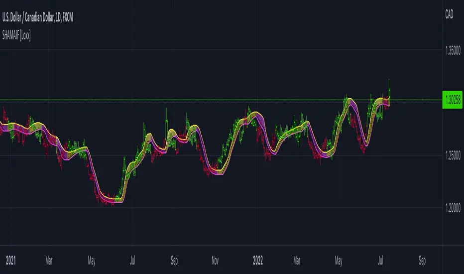
Jurik Filter TRIX Log [Loxx]Jurik Filter TRIX Log is a TRIX indicator that calculates TRIX using a Jurik Filter instead of EMA. this indicator responds much quicker than traditional TRIX.
What is TRIX?
TRIX is a momentum oscillator that displays the percent rate of change of a TEMA. It was developed in the early 1980's by Jack Hutson, an editor for "Technical Analysis of Stocks and Commodities" magazine. With its triple smoothing, TRIX is designed to filter insignificant price movements. In his article he uses a logarithm of a price (which is in many versions, left out).
What is Jurik Volty used in the Juirk Filter?
One of the lesser known qualities of Juirk smoothing is that the Jurik smoothing process is adaptive. "Jurik Volty" (a sort of market volatility ) is what makes Jurik smoothing adaptive. The Jurik Volty calculation can be used as both a standalone indicator and to smooth other indicators that you wish to make adaptive.
What is the Jurik Moving Average?
Have you noticed how moving averages add some lag (delay) to your signals? ... especially when price gaps up or down in a big move, and you are waiting for your moving average to catch up? Wait no more! JMA eliminates this problem forever and gives you the best of both worlds: low lag and smooth lines.
Included:
-Bar coloring
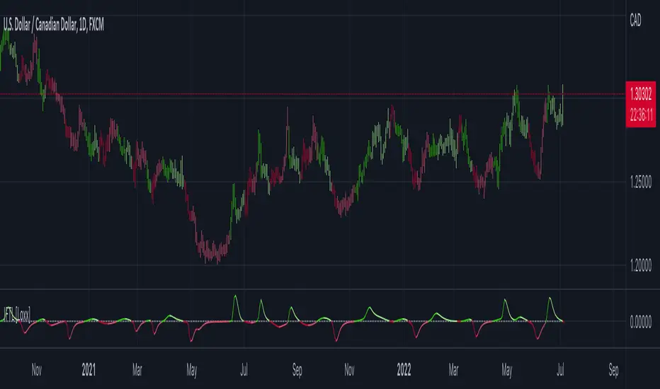
Jurik Filtered Perfect CCI (PCCI) [Loxx]Jurik Filtered Perfect CCI (PCCI) is a faster and more accurate version of CCI with Jurik Filtering.
What is the PCCI (Perfect Commodity Channel Index)?
PCCI (Perfect Commodity Channel Index) indicator is calculated by the following formula:
PCCI(bar) = close(bar) – DF(bar)
PCCI resembles D. Lambert's Commodity Channel Index by the method of its calculation.
Actually, CCI index is calculated as a normalized difference between the current price and its moving average. PCCI is calculated as a difference between a day closing price and its statistical expectation presented by a Digital Fitler value. Therefore, PCCI is more efficient than CCI.
PCCI index is a high frequency part of the exchange rate fluctuations normalized according to its standard deviation.
What is Jurik Volty used in the Juirk Filter?
One of the lesser known qualities of Juirk smoothing is that the Jurik smoothing process is adaptive. "Jurik Volty" (a sort of market volatility ) is what makes Jurik smoothing adaptive. The Jurik Volty calculation can be used as both a standalone indicator and to smooth other indicators that you wish to make adaptive.
What is the Jurik Moving Average?
Have you noticed how moving averages add some lag (delay) to your signals? ... especially when price gaps up or down in a big move, and you are waiting for your moving average to catch up? Wait no more! JMA eliminates this problem forever and gives you the best of both worlds: low lag and smooth lines.
Ideally, you would like a filtered signal to be both smooth and lag-free. Lag causes delays in your trades, and increasing lag in your indicators typically result in lower profits. In other words, late comers get what's left on the table after the feast has already begun.
Included:
-Bar coloring
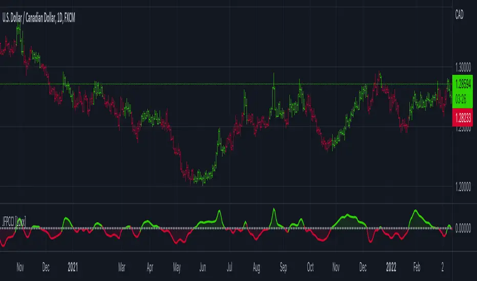
CFB Adaptive MOGALEF Bands [Loxx]A Pine Script adaptation from MOGALEF Bands .
What are MOGALEF Bands?
Actual MOGALEF bands code is the final result of a lot of contributors. Syllables MO-GA-LEF are the initials of three of them.
The basic idea of bands: the markets are still in range, and trends that are moving ranges. The Mogalef bands try to estimate the current range and to project its on the future if prices move. This future estimation is often of great relevance and very useful, especialy for market profile users or pivot points users.
What is Composite Fractal Behavior ( CFB )?
All around you mechanisms adjust themselves to their environment. From simple thermostats that react to air temperature to computer chips in modern cars that respond to changes in engine temperature, r.p.m.'s, torque, and throttle position. It was only a matter of time before fast desktop computers applied the mathematics of self-adjustment to systems that trade the financial markets.
Unlike basic systems with fixed formulas, an adaptive system adjusts its own equations. For example, start with a basic channel breakout system that uses the highest closing price of the last N bars as a threshold for detecting breakouts on the up side. An adaptive and improved version of this system would adjust N according to market conditions, such as momentum, price volatility or acceleration.
Since many systems are based directly or indirectly on cycles, another useful measure of market condition is the periodic length of a price chart's dominant cycle, (DC), that cycle with the greatest influence on price action.
The utility of this new DC measure was noted by author Murray Ruggiero in the January '96 issue of Futures Magazine. In it. Mr. Ruggiero used it to adaptive adjust the value of N in a channel breakout system. He then simulated trading 15 years of D-Mark futures in order to compare its performance to a similar system that had a fixed optimal value of N. The adaptive version produced 20% more profit!
This DC index utilized the popular MESA algorithm (a formulation by John Ehlers adapted from Burg's maximum entropy algorithm, MEM). Unfortunately, the DC approach is problematic when the market has no real dominant cycle momentum, because the mathematics will produce a value whether or not one actually exists! Therefore, we developed a proprietary indicator that does not presuppose the presence of market cycles. It's called CFB (Composite Fractal Behavior) and it works well whether or not the market is cyclic.
CFB examines price action for a particular fractal pattern, categorizes them by size, and then outputs a composite fractal size index. This index is smooth, timely and accurate
Essentially, CFB reveals the length of the market's trending action time frame. Long trending activity produces a large CFB index and short choppy action produces a small index value. Investors have found many applications for CFB which involve scaling other existing technical indicators adaptively, on a bar-to-bar basis.
What is Jurik Volty used in the Juirk Filter?
One of the lesser known qualities of Juirk smoothing is that the Jurik smoothing process is adaptive. "Jurik Volty" (a sort of market volatility ) is what makes Jurik smoothing adaptive. The Jurik Volty calculation can be used as both a standalone indicator and to smooth other indicators that you wish to make adaptive.
What is the Jurik Moving Average?
Have you noticed how moving averages add some lag (delay) to your signals? ... especially when price gaps up or down in a big move, and you are waiting for your moving average to catch up? Wait no more! JMA eliminates this problem forever and gives you the best of both worlds: low lag and smooth lines.
Ideally, you would like a filtered signal to be both smooth and lag-free. Lag causes delays in your trades, and increasing lag in your indicators typically result in lower profits. In other words, late comers get what's left on the table after the feast has already begun.
Included:
-Color bars
-Fill levels

CFB Adaptive Gann HiLo Activator Histogram [Loxx]CFB Adaptive Gann HiLo Activator Histogram is a Composite-Fractal-Behavior-adaptive Gann HiLo activator in histogram form that has been smoothed using Jurik Filtering to reduce noise and better identify trending markets. This indicator is the CFB adaptive version of Jurik-Filtered, Gann HiLo Activator .
What is Gann HiLo
The HiLo Activator study is a trend-following indicator introduced by Robert Krausz as part of the Gann Swing trading strategy. In addition to indicating the current trend direction, this can be used as both entry signal and trailing stop.
Here is how the HiLo Activator is calculated:
1. The system calculates the moving averages of the high and low prices over the last several candles. By default, the average is calculated using the last three candles.
2. If the close price falls below the average low or rises above the average high, the system plots the opposite moving average. For example, if the price crosses above the average high, the system will plot the average low. If the price crosses below the average low afterward, the system will stop plotting the average low and will start plotting the average high, and so forth .
The plot of the HiLo Activator thus consists of sections on the top and bottom of the price plot. The sections on the bottom signify bullish trending conditions. Vice versa, those on the top signify the bearish conditions.
What is Composite Fractal Behavior ( CFB )?
All around you mechanisms adjust themselves to their environment. From simple thermostats that react to air temperature to computer chips in modern cars that respond to changes in engine temperature, r.p.m.'s, torque, and throttle position. It was only a matter of time before fast desktop computers applied the mathematics of self-adjustment to systems that trade the financial markets.
Unlike basic systems with fixed formulas, an adaptive system adjusts its own equations. For example, start with a basic channel breakout system that uses the highest closing price of the last N bars as a threshold for detecting breakouts on the up side. An adaptive and improved version of this system would adjust N according to market conditions, such as momentum, price volatility or acceleration.
Since many systems are based directly or indirectly on cycles, another useful measure of market condition is the periodic length of a price chart's dominant cycle, (DC), that cycle with the greatest influence on price action.
The utility of this new DC measure was noted by author Murray Ruggiero in the January '96 issue of Futures Magazine. In it. Mr. Ruggiero used it to adaptive adjust the value of N in a channel breakout system. He then simulated trading 15 years of D-Mark futures in order to compare its performance to a similar system that had a fixed optimal value of N. The adaptive version produced 20% more profit!
This DC index utilized the popular MESA algorithm (a formulation by John Ehlers adapted from Burg's maximum entropy algorithm, MEM). Unfortunately, the DC approach is problematic when the market has no real dominant cycle momentum, because the mathematics will produce a value whether or not one actually exists! Therefore, we developed a proprietary indicator that does not presuppose the presence of market cycles. It's called CFB (Composite Fractal Behavior) and it works well whether or not the market is cyclic.
CFB examines price action for a particular fractal pattern, categorizes them by size, and then outputs a composite fractal size index. This index is smooth, timely and accurate
Essentially, CFB reveals the length of the market's trending action time frame. Long trending activity produces a large CFB index and short choppy action produces a small index value. Investors have found many applications for CFB which involve scaling other existing technical indicators adaptively, on a bar-to-bar basis.
What is Jurik Volty used in the Juirk Filter?
One of the lesser known qualities of Juirk smoothing is that the Jurik smoothing process is adaptive. "Jurik Volty" (a sort of market volatility ) is what makes Jurik smoothing adaptive. The Jurik Volty calculation can be used as both a standalone indicator and to smooth other indicators that you wish to make adaptive.
What is the Jurik Moving Average?
Have you noticed how moving averages add some lag (delay) to your signals? ... especially when price gaps up or down in a big move, and you are waiting for your moving average to catch up? Wait no more! JMA eliminates this problem forever and gives you the best of both worlds: low lag and smooth lines.
Ideally, you would like a filtered signal to be both smooth and lag-free. Lag causes delays in your trades, and increasing lag in your indicators typically result in lower profits. In other words, late comers get what's left on the table after the feast has already begun.
Included
-Toggle bar color on/off
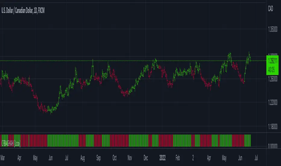
Jurik CFB Adaptive, Elder Force Index w/ ATR Channels [Loxx]Jurik CFB Adaptive, Elder Force Index w/ ATR Channels is a variation of Elder Force Index that better adapts to trends by calculating dynamic lengths for the traditional Elder Force Index calculation. ATR channels are added to show levels of price extremes or exhaustion of price either up or down. Elder Force Index is typically used for spotting reversals on the weekly timeframe.
What is the Elder Force Index?
Dr. Alexander Elder is one of the contributors to a newer generation of technical indicators. His force index is an oscillator that measures the force, or power, of bulls behind particular market rallies and of bears behind every decline.1
The three key components of the force index are the direction of price change, the extent of the price change, and the trading volume. When the force index is used in conjunction with a moving average, the resulting figure can accurately measure significant changes in the power of bulls and bears.1 In this way, Elder has taken an extremely useful solitary indicator, the moving average, and combined it with his force index for even greater predictive success.
What is Composite Fractal Behavior ( CFB )?
All around you mechanisms adjust themselves to their environment. From simple thermostats that react to air temperature to computer chips in modern cars that respond to changes in engine temperature, r.p.m.'s, torque, and throttle position. It was only a matter of time before fast desktop computers applied the mathematics of self-adjustment to systems that trade the financial markets.
Unlike basic systems with fixed formulas, an adaptive system adjusts its own equations. For example, start with a basic channel breakout system that uses the highest closing price of the last N bars as a threshold for detecting breakouts on the up side. An adaptive and improved version of this system would adjust N according to market conditions, such as momentum, price volatility or acceleration.
Since many systems are based directly or indirectly on cycles, another useful measure of market condition is the periodic length of a price chart's dominant cycle, (DC), that cycle with the greatest influence on price action.
The utility of this new DC measure was noted by author Murray Ruggiero in the January '96 issue of Futures Magazine. In it. Mr. Ruggiero used it to adaptive adjust the value of N in a channel breakout system. He then simulated trading 15 years of D-Mark futures in order to compare its performance to a similar system that had a fixed optimal value of N. The adaptive version produced 20% more profit!
This DC index utilized the popular MESA algorithm (a formulation by John Ehlers adapted from Burg's maximum entropy algorithm, MEM). Unfortunately, the DC approach is problematic when the market has no real dominant cycle momentum, because the mathematics will produce a value whether or not one actually exists! Therefore, we developed a proprietary indicator that does not presuppose the presence of market cycles. It's called CFB (Composite Fractal Behavior) and it works well whether or not the market is cyclic.
CFB examines price action for a particular fractal pattern, categorizes them by size, and then outputs a composite fractal size index. This index is smooth, timely and accurate
Essentially, CFB reveals the length of the market's trending action time frame. Long trending activity produces a large CFB index and short choppy action produces a small index value. Investors have found many applications for CFB which involve scaling other existing technical indicators adaptively, on a bar-to-bar basis.
What is Jurik Volty used in the Juirk Filter?
One of the lesser known qualities of Juirk smoothing is that the Jurik smoothing process is adaptive. "Jurik Volty" (a sort of market volatility ) is what makes Jurik smoothing adaptive. The Jurik Volty calculation can be used as both a standalone indicator and to smooth other indicators that you wish to make adaptive.
What is the Jurik Moving Average?
Have you noticed how moving averages add some lag (delay) to your signals? ... especially when price gaps up or down in a big move, and you are waiting for your moving average to catch up? Wait no more! JMA eliminates this problem forever and gives you the best of both worlds: low lag and smooth lines.
Ideally, you would like a filtered signal to be both smooth and lag-free. Lag causes delays in your trades, and increasing lag in your indicators typically result in lower profits. In other words, late comers get what's left on the table after the feast has already begun.

CFB Adaptive, Jurik-Filtered Gann HiLo Activator [Loxx]CFB Adaptive, Jurik-Filtered Gann HiLo Activator is a Composite-Fractal-Behavior-adaptive Gann HiLo activator that has been smoothed using Jurik Filtering to reduce noise and better identify trending markets. This indicator is the CFB adaptive version of Jurik-Filtered, Gann HiLo Activator .
What is Gann HiLo
The HiLo Activator study is a trend-following indicator introduced by Robert Krausz as part of the Gann Swing trading strategy. In addition to indicating the current trend direction, this can be used as both entry signal and trailing stop.
Here is how the HiLo Activator is calculated:
1. The system calculates the moving averages of the high and low prices over the last several candles. By default, the average is calculated using the last three candles.
2. If the close price falls below the average low or rises above the average high, the system plots the opposite moving average. For example, if the price crosses above the average high, the system will plot the average low. If the price crosses below the average low afterward, the system will stop plotting the average low and will start plotting the average high, and so forth .
The plot of the HiLo Activator thus consists of sections on the top and bottom of the price plot. The sections on the bottom signify bullish trending conditions. Vice versa, those on the top signify the bearish conditions.
What is Composite Fractal Behavior (CFB)?
All around you mechanisms adjust themselves to their environment. From simple thermostats that react to air temperature to computer chips in modern cars that respond to changes in engine temperature, r.p.m.'s, torque, and throttle position. It was only a matter of time before fast desktop computers applied the mathematics of self-adjustment to systems that trade the financial markets.
Unlike basic systems with fixed formulas, an adaptive system adjusts its own equations. For example, start with a basic channel breakout system that uses the highest closing price of the last N bars as a threshold for detecting breakouts on the up side. An adaptive and improved version of this system would adjust N according to market conditions, such as momentum, price volatility or acceleration.
Since many systems are based directly or indirectly on cycles, another useful measure of market condition is the periodic length of a price chart's dominant cycle, (DC), that cycle with the greatest influence on price action.
The utility of this new DC measure was noted by author Murray Ruggiero in the January '96 issue of Futures Magazine. In it. Mr. Ruggiero used it to adaptive adjust the value of N in a channel breakout system. He then simulated trading 15 years of D-Mark futures in order to compare its performance to a similar system that had a fixed optimal value of N. The adaptive version produced 20% more profit!
This DC index utilized the popular MESA algorithm (a formulation by John Ehlers adapted from Burg's maximum entropy algorithm, MEM). Unfortunately, the DC approach is problematic when the market has no real dominant cycle momentum, because the mathematics will produce a value whether or not one actually exists! Therefore, we developed a proprietary indicator that does not presuppose the presence of market cycles. It's called CFB (Composite Fractal Behavior) and it works well whether or not the market is cyclic.
CFB examines price action for a particular fractal pattern, categorizes them by size, and then outputs a composite fractal size index. This index is smooth, timely and accurate
Essentially, CFB reveals the length of the market's trending action time frame. Long trending activity produces a large CFB index and short choppy action produces a small index value. Investors have found many applications for CFB which involve scaling other existing technical indicators adaptively, on a bar-to-bar basis.
What is Jurik Volty used in the Juirk Filter?
One of the lesser known qualities of Juirk smoothing is that the Jurik smoothing process is adaptive. "Jurik Volty" (a sort of market volatility ) is what makes Jurik smoothing adaptive. The Jurik Volty calculation can be used as both a standalone indicator and to smooth other indicators that you wish to make adaptive.
What is the Jurik Moving Average?
Have you noticed how moving averages add some lag (delay) to your signals? ... especially when price gaps up or down in a big move, and you are waiting for your moving average to catch up? Wait no more! JMA eliminates this problem forever and gives you the best of both worlds: low lag and smooth lines.
Ideally, you would like a filtered signal to be both smooth and lag-free. Lag causes delays in your trades, and increasing lag in your indicators typically result in lower profits. In other words, late comers get what's left on the table after the feast has already begun.
Included
-Toggle bar color on/off
