Jurik Moving Average (JMA)Overview
Jurik Moving Average (JMA) is an adaptive moving average developed by Mark Jurik, widely regarded as one of the most powerful moving averages available to traders. This implementation provides a direct Pine Script translation of the reverse-engineered JMA algorithm
What Makes JMA Special
Unlike traditional moving averages, JMA adapts to market volatility in real-time. This "triple adaptive" approach allows JMA to:
Reduce lag significantly while maintaining exceptional smoothness
React quickly during trending markets
Filter out noise during consolidation phases
Provide clearer trend signals with fewer whipsaws
The Triple Adaptive Edge
JMA employs a three-stage smoothing process:
Preliminary smoothing via an adaptive EMA
Secondary smoothing using a Kalman filter with phase adjustment
Final smoothing through a unique Jurik adaptive filter
This approach combines with a dynamic volatility-based factor (alpha) that adapts to market conditions, making JMA superior to traditional moving averages in most situations.
Key Parameters
Period : Controls the lookback period (default: 14)
Phase : Adjusts the heaviness of the indicator (-100 to 100, default: 0)
Positive values reduce lag but may cause overshoot
Negative values increase smoothness but reduce responsiveness
Power : Smoothing factor (0.1-0.9, default 0.45)
Higher values create smoother curves
Lower values create more responsive but choppy curves
Jurik

JMA Quantum Edge: Adaptive Precision Trading System JMA Quantum Edge: Adaptive Precision Trading System - Enhanced Visuals & Risk Management
Get ready to experience a groundbreaking trading strategy that adapts in real-time to market conditions! This powerful, open-source script combines advanced technical analysis with state-of-the-art risk management tools, designed to give you the edge you need in today's dynamic markets.
What It Does:
Adaptive JMA Indicator:
Utilizes a custom Jurik Moving Average (JMA) that adjusts its sensitivity based on market volatility, ensuring you get precise signals even in the most fluctuating environments.
Dynamic Risk Management:
Features built-in support for partial exits (scaling out) to secure profits, along with an optional Kelly Criterion-based position sizing that tailors your exposure based on historical performance metrics.
Robust Error Handling:
Incorporates market condition filters—like minimum volume and maximum allowed gap percentage—to ensure trades are only executed under favorable conditions.
Vivid Visual Enhancements:
Enjoy an animated background that reflects market momentum, dynamic pivot markers, and clearly drawn trend channels. Plus, interactive tables provide real-time performance analytics and detailed error metrics.
Fully Customizable:
With a comprehensive set of inputs, you can easily tailor the strategy to your personal trading style and market preferences. Adjust everything from JMA parameters to refresh intervals for tables and labels!
How to Use It:
Add the Script:
Copy and paste the script into the Pine Script Editor on TradingView and click “Add to Chart.”
Configure Your Settings:
Customize your risk management (capital, commission, position sizing, partial exits, etc.) and tweak the JMA settings to match your preferred trading style. Use the extensive input panel to adjust visuals, alerts, and more.
Backtest & Optimize:
Run the strategy in the Strategy Tester to analyze its historical performance. Monitor real-time analytics and error metrics via the interactive tables, and fine-tune your parameters for optimal performance.
Go Live with Confidence:
Once you're satisfied with the backtest results, use the generated signals for live trading, and let the system help you stay ahead in fast-paced markets!
How to use the imputs:
This cutting-edge strategy is designed to adapt to changing market conditions and offers you complete control over your trading parameters. Here’s a breakdown of what each group of inputs does and how you should use them:
Risk Management & Trade Settings
Recalculate on Every Tick:
What it does: When enabled, the strategy recalculates on every price update.
Recommendation: Leave it true for fast charts.
Initial Capital:
What it does: Sets your starting capital for backtesting, which influences position sizing and performance metrics.
Recommendation: Start with $10,000 (or adjust according to your trading capital).
Commission (%):
What it does: Simulates the cost per trade.
Recommendation: Use a realistic rate (e.g., 0.04%).
Position Size & Quantity Type:
What they do: Define how large each trade will be. Choose between a fixed unit amount or a percentage of equity.
Recommendation: For beginners, the default fixed value is a good start. Experiment later with percentage-based sizing if needed.
Order Comment:
What it does: Adds a label to your orders for easier tracking.
Allow Reverse Orders:
What it does: If disabled, the strategy will close opposing positions before entering a new trade, reducing conflicts.
Enable Dynamic Position Sizing:
What it does: Adjusts trade size based on current volatility.
Recommendation: Beginners may start with this disabled until they understand basic sizing.
Partial Exit Inputs:
What they do:
Enable Partial Exits: When turned on, you can scale out of your position to lock in profits.
Partial Exit Profit (%): The profit percentage that triggers a partial exit.
Partial Exit Percentage: The percentage of your current position to exit. Recommendation: Use defaults (e.g., 5% profit, 50% exit) to secure profits gradually.
Kelly Criterion Option:
What it does: When enabled, adjusts your position sizing using historical performance (win rate and profit factor).
Recommendation: Beginners might leave this disabled until comfortable with backtest performance metrics.
Market Condition Filters:
What they do:
Minimum Volume: Ensures trades occur only when there’s sufficient market activity.
Maximum Gap (%): Prevents trading if there’s an unusually large gap between the previous close and current open. Recommendation: Defaults work well for most markets. If trades seem erratic, consider tightening these limits.
JMA Settings
Price Source:
What it does: The input series for the JMA calculation, typically set to the closing price.
JMA Length:
What it does: Controls the smoothing period of the JMA. Lower values are more sensitive; higher values smooth out the noise. Recommendation: Start with 21.
JMA Phase & Power:
What they do: Adjust how responsive the JMA is. Phase controls timing; power adjusts the intensity. Recommendation: Default settings (63 phase and 3 power) are a balanced starting point.
Visual Settings & Style
Show JMA Line, Pivot Lines, and Pivot Labels:
What they do: Toggle visual elements on your chart for easier signal identification.
Pivot History Count:
What it does: Limits how many historical pivot markers are displayed.
Color Settings (Up/Down Neon Colors):
What they do: Set the visual cues for buy and sell signals.
Pivot Marker & Line Style:
What they do: Choose the style and thickness of your pivot markers and lines.
Show Stats Panel:
What it does: Displays real-time performance and error metrics.
Dynamic Background & Visual Enhancements
Animate Background:
What it does: Changes the background color based on market momentum.
Show Trend Channels & Volume Zones:
What they do: Draw trend channels and highlight areas of high volatility/volume.
Show Data-Rich Labels:
What it does: Displays key metrics like volume, error percentage, and momentum on the chart.
High Volatility Threshold:
What it does: Determines the multiplier for when the chart background should change due to high volatility.
Multi-Timeframe Settings
Higher Timeframe:
What it does: Uses a higher timeframe’s JMA for trend confirmation. Recommendation: Use Daily ('D') or Weekly ('W') for broader trend analysis.
Show HTF Trend Zone & Opacity:
What they do: Display a visual zone from the higher timeframe to help confirm trends.
6. Trailing Stop Settings
Trailing Stop ATR Factor & Offset Multiplier:
What they do: Calculate trailing stops based on the Average True Range (ATR), adjusting stop distances dynamically. Recommendation: Default settings are a good balance but can be fine-tuned based on asset volatility.
Alerts & Notifications
Alerts on Pivot Formation & JMA Crossover:
What they do: Notify you when key events occur.
Dynamic Power Threshold:
What it does: Sets the sensitivity for dynamic alerts.
8. Static Stop Loss / Take Profit
Static Stop Loss (%) & Take Profit (%):
What they do: Allow you to set fixed stop loss or take profit levels. Recommendation: Leave them at 0 to disable if you prefer dynamic risk management, or set them if you have strict risk/reward preferences.
Advanced Settings
ATR Length:
What it does: Determines the period for ATR calculation, impacting trailing stop sensitivity. Recommendation: Start with 14.
Optimization Feedback & Enhanced Error Analysis
Error Metric Length & Error Threshold (%):
What they do: Calculate error metrics (like average error, skewness, and kurtosis) to help you fine-tune the JMA. Recommendation: Use the defaults and adjust if the error metrics seem off during backtesting.
UI - User-Driven Tweaking & Table Customization
Parameter Tweaker Panel, Debug/Performance Table Settings:
What they do: Provide interactive tables that display real-time performance, error metrics, and allow you to monitor strategy parameters.
Refresh Frequency Options (Table & Label Refresh Intervals):
What they do: Set how often the tables and labels update.
Recommendation: Start with an interval of 1 bar; increase it if your chart is too busy.
Important for Beginners:
Default Settings:
All default values have been chosen for balanced performance across different markets. If you ever experience unexpected behavior, start by resetting the inputs to their defaults.
Step-by-Step Adjustments:
Experiment by changing one setting at a time while observing how the strategy’s signals and performance metrics change. This will help you understand the impact of each parameter.
Resetting to Defaults:
If things seem off or you’re not getting the expected results, you can always reset the indicator. Either reload the script or use the “Reset Inputs” option (if available) to revert to the default settings.
Jump in, experiment, and enjoy the power of adaptive precision trading. This strategy is built to grow with your skills—have fun exploring and refining your trading edge!
Happy trading!

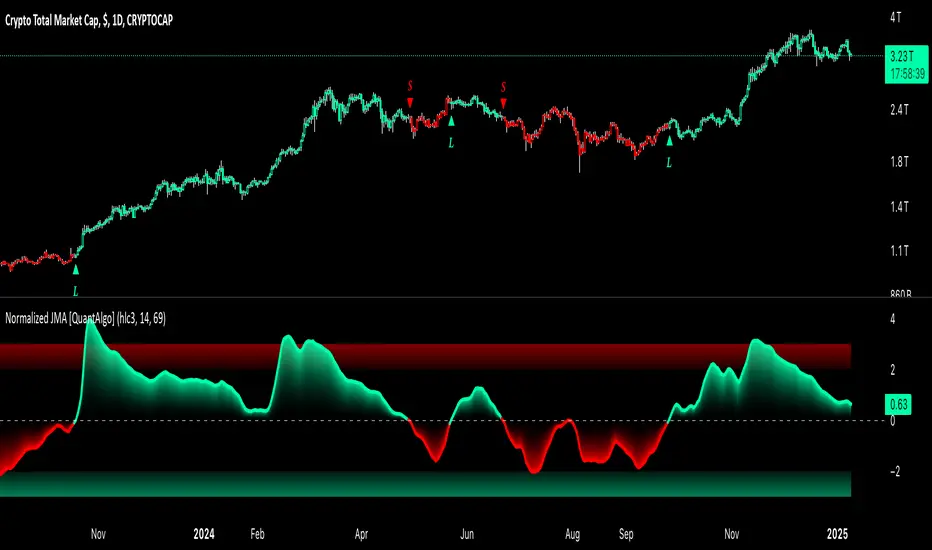
Normalized Jurik Moving Average [QuantAlgo]Upgrade your investing and trading strategy with the Normalized Jurik Moving Average (JMA) , a sophisticated oscillator that combines adaptive smoothing with statistical normalization to deliver high-quality signals! Whether you're a swing trader looking for momentum shifts or a medium- to long-term investor focusing on trend validation, this indicator's statistical approach offers valuable analytical advantages that can enhance your trading and investing decisions!
🟢 Core Architecture
The foundation of this indicator lies in its unique dual-layer calculation system. The first layer implements the Jurik Moving Average, known for its superior noise reduction and responsiveness, while the second layer applies statistical normalization (Z-Score) to create standardized readings. This sophisticated approach helps identify significant price movements while filtering out market noise across various timeframes and instruments.
🟢 Technical Foundation
Three key components power this indicator are:
Jurik Moving Average (JMA): An advanced moving average calculation that provides superior smoothing with minimal lag
Statistical Normalization: Z-Score based scaling that creates consistent, comparable readings across different market conditions
Dynamic Zone Detection: Automatically identifies overbought and oversold conditions based on statistical deviations
🟢 Key Features & Signals
The Normalized JMA delivers market insights through:
Color-adaptive oscillator line that reflects momentum strength and direction
Statistically significant overbought/oversold zones for trade validation
Smart gradient fills between signal line and zero level for enhanced visualization
Clear long (L) and short (S) markers for validated momentum shifts
Intelligent bar coloring that highlights the current market state
Customizable alert system for both bullish and bearish setups
🟢 Practical Usage Tips
Here's how to maximize your use of the Normalized JMA:
1/ Setup:
Add the indicator to your favorites, then apply it to your chart ⭐️
Begin with the default smoothing period for balanced analysis
Use the default normalization period for optimal signal generation
Start with standard visualization settings
Customize colors to match your chart preferences
Enable both bar coloring and signal markers for complete visual feedback
2/ Reading Signals:
Watch for L/S markers - they indicate validated momentum shifts
Monitor oscillator line color changes for direction confirmation
Use the built-in alert system to stay informed of potential trend changes
🟢 Pro Tips
Adjust Smoothing Period based on your trading style:
→ Lower values (8-12) for more responsive signals
→ Higher values (20-30) for more stable trend identification
Fine-tune Normalization Period based on market conditions:
→ Shorter periods (20-25) for more dynamic markets
→ Longer periods (40-50) for more stable markets
Optimize your analysis by:
→ Using +2/-2 zones for primary trade signals
→ Using +3/-3 zones for extreme market conditions
→ Combining with volume analysis for trade confirmation
→ Using multiple timeframe analysis for strategic context
Combine with:
→ Volume indicators for trade validation
→ Price action for entry timing
→ Support/resistance levels for profit targets
→ Trend-following indicators for directional bias
Dynamic Jurik RSX w/ Fisher Transform█ Introduction
The Dynamic Jurik RSX with Fisher Transform is a powerful and adaptive momentum indicator designed for traders who seek a non-laggy view of price movements. This script is based on the classic Jurik RSX (Relative Strength Index). It also includes features such as the dynamic overbought and oversold limits, the Inverse Fisher Transform, trend display, slope calculations, and the ability to color extremes for better clarity.
█ Key Features:
• RSX: The Relative Strength Index (RSX) in this script is based on Jurik’s RSX, which is smoother than the traditional RSI and aims to reduce noise and lag. This script calculates the RSX using an exponential smoothing technique and adaptive adjustments.
• Inverse Fisher Transform: This script can optionally apply the Inverse Fisher Transform to the RSX, which helps to normalize the RSX values, compressing them between -1 and 1. The inverse transformation makes it easier to spot extreme values (overbought and oversold conditions) by enhancing the visual clarity of those extremes. It also smooths the curve over a user-defined period in hopes of providing a more consistent signal.
• Dynamic Limits: The dynamic overbought and oversold limits are calculated based on the RSX's recent high and low values. The limits adjust dynamically depending on market conditions, making them more relevant to current price action.
• Slope Display: The slope of the RSX is calculated as the rate of change between the current and previous RSX value. The slope is displayed as dots when the slope exceeds the threshold designated by the user, providing visual cues for momentum shifts.
• Trend Coloring: Optionally, the user can also enable a trend-based display. It is simply based on current value of RSX versus the previous one. If RSX is rising then the trend is bullish, if not, then the trend is bearish.
• Coloring Extremes: Users can configure the RSX to color the chart when prices enter extreme conditions, such as overbought or oversold zones, providing visual cues for market reversals.
█ Attached Chart Notes:
• Top Panel: Enabled dynamic limits, Trend display, standard Jurik RSX with 20 lookback period, and Slope display.
• Middle Panel: Enabled dynamic limits, Extremes display, and standard Jurik RSX with 20 lookback period.
• Bottom Panel: Enabled dynamic limits, Trend display, Inverse Fisher Transform with 14 lookback period and 9 smoothing period. and Slope display.
█ Credits:
Special thanks to Everget for providing the original script. The script was also slightly modified based on updates from outside sources.
█ Disclaimer:
This script is for educational purposes only and should not be considered financial advice. Always conduct your own research and consult a professional before making any trading decisions.

Goertzel Adaptive JMA T3Hello Fellas,
The Goertzel Adaptive JMA T3 is a powerful indicator that combines my own created Goertzel adaptive length with Jurik and T3 Moving Averages. The primary intention of the indicator is to demonstrate the new adaptive length algorithm by applying it on bleeding-edge MAs.
It is useable like any moving average, and the new Goertzel adaptive length algorithm can be used to make own indicators Goertzel adaptive.
Used Adaptive Length Algorithms
Normalized Goertzel Power: This uses the normalized power of the Goertzel algorithm to compute an adaptive length without the special operations, like detrending, Ehlers uses for his DFT adaptive length.
Ehlers Mod: This uses the Goertzel algorithm instead of the DFT, originally used by Ehlers, to compute a modified version of his original approach, which sticks as close as possible to the original approach.
Scoring System
The scoring system determines if bars are red or green and collects them.
Then, it goes through all collected red and green bars and checks how big they are and if they are above or below the selected MA. It is positive when green bars are under MA or when red bars are above MA.
Then, it accumulates the size for all positive green bars and for all positive red bars. The same happens for negative green and red bars.
Finally, it calculates the score by ((positiveGreenBars + positiveRedBars) / (negativeGreenBars + negativeRedBars)) * 100 with the scale 0–100.
Signals
Is the price above MA? -> bullish market
Is the price below MA? -> bearish market
Usage
Adjust the settings to reach the highest score, and enjoy an outstanding adaptive MA.
It should be useable on all timeframes. It is recommended to use the indicator on the timeframe where you can get the highest score.
Now, follows a bunch of knowledge for people who don't know about the concepts used here.
T3
The T3 moving average, short for "Tim Tillson's Triple Exponential Moving Average," is a technical indicator used in financial markets and technical analysis to smooth out price data over a specific period. It was developed by Tim Tillson, a software project manager at Hewlett-Packard, with expertise in Mathematics and Computer Science.
The T3 moving average is an enhancement of the traditional Exponential Moving Average (EMA) and aims to overcome some of its limitations. The primary goal of the T3 moving average is to provide a smoother representation of price trends while minimizing lag compared to other moving averages like Simple Moving Average (SMA), Weighted Moving Average (WMA), or EMA.
To compute the T3 moving average, it involves a triple smoothing process using exponential moving averages. Here's how it works:
Calculate the first exponential moving average (EMA1) of the price data over a specific period 'n.'
Calculate the second exponential moving average (EMA2) of EMA1 using the same period 'n.'
Calculate the third exponential moving average (EMA3) of EMA2 using the same period 'n.'
The formula for the T3 moving average is as follows:
T3 = 3 * (EMA1) - 3 * (EMA2) + (EMA3)
By applying this triple smoothing process, the T3 moving average is intended to offer reduced noise and improved responsiveness to price trends. It achieves this by incorporating multiple time frames of the exponential moving averages, resulting in a more accurate representation of the underlying price action.
JMA
The Jurik Moving Average (JMA) is a technical indicator used in trading to predict price direction. Developed by Mark Jurik, it’s a type of weighted moving average that gives more weight to recent market data rather than past historical data.
JMA is known for its superior noise elimination. It’s a causal, nonlinear, and adaptive filter, meaning it responds to changes in price action without introducing unnecessary lag. This makes JMA a world-class moving average that tracks and smooths price charts or any market-related time series with surprising agility.
In comparison to other moving averages, such as the Exponential Moving Average (EMA), JMA is known to track fast price movement more accurately. This allows traders to apply their strategies to a more accurate picture of price action.
Goertzel Algorithm
The Goertzel algorithm is a technique in digital signal processing (DSP) for efficient evaluation of individual terms of the Discrete Fourier Transform (DFT). It's particularly useful when you need to compute a small number of selected frequency components. Unlike direct DFT calculations, the Goertzel algorithm applies a single real-valued coefficient at each iteration, using real-valued arithmetic for real-valued input sequences. This makes it more numerically efficient when computing a small number of selected frequency components¹.
Discrete Fourier Transform
The Discrete Fourier Transform (DFT) is a mathematical technique used in signal processing to convert a finite sequence of equally-spaced samples of a function into a same-length sequence of equally-spaced samples of the discrete-time Fourier transform (DTFT), which is a complex-valued function of frequency . The DFT provides a frequency domain representation of the original input sequence .
Usage of DFT/Goertzel In Adaptive Length Algorithms
Adaptive length algorithms are automated trading systems that can dynamically adjust their parameters in response to real-time market data. This adaptability enables them to optimize their trading strategies as market conditions fluctuate. Both the Goertzel algorithm and DFT can be used in these algorithms to analyze market data and detect cycles or patterns, which can then be used to adjust the parameters of the trading strategy.
The Goertzel algorithm is more efficient than the DFT when you need to compute a small number of selected frequency components. However, for covering a full spectrum, the Goertzel algorithm has a higher order of complexity than fast Fourier transform (FFT) algorithms.
I hope this can help you somehow.
Thanks for reading, and keep it up.
Best regards,
simwai
---
Credits to:
@ClassicScott
@yatrader2
@cheatcountry
@loxx

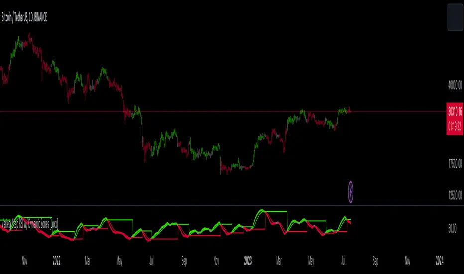
Variety Step RSI w/ Dynamic Zones [Loxx]Variety Step RSI w/ Dynamic Zones is a stepped RSI calculation with Discontinued Signal Lines. This indicator includes 7 types of RSI to choose from. The addition of the Discontinued Signal Lines allows this indicator to better identify momentum shifts in price so traders have better defined long/short signals.
Enhanced Moving Average Calculation with Stepped Moving Average and the Advantages over Regular RSI
Technical analysis plays a crucial role in understanding and predicting market trends. One popular indicator used by traders and analysts is the Relative Strength Index (RSI). However, an enhanced approach called Stepped Moving Average, in combination with the Slow RSI function, offers several advantages over regular RSI calculations.
█ Stepped Moving Average and Moving Averages:
The Stepped Moving Average function serves as a crucial component in the calculation of moving averages. Moving averages smooth out price data over a specific period to identify trends and potential trading signals. By employing the Stepped Moving Average function, traders can enhance the accuracy of moving averages and make more informed decisions.
Stepped Moving Average takes two parameters:
The current RSI value and a size parameter. It computes the next step in the moving average calculation by determining the upper and lower bounds of the moving average range. It accomplishes this by adjusting the values of smax and smin based on the given RSI and size.
Furthermore, Stepped Moving Average introduces the concept of a trend variable. By comparing the previous trend value with the current RSI and the previous upper and lower bounds, it updates the trend accordingly. This feature enables traders to identify potential shifts in market sentiment and make timely adjustments to their trading strategies.
█ Advantages over Regular RSI:
Enhanced Range Boundaries:
The inclusion of size parameters in Stepped Moving Average allows for more precise determination of the upper and lower bounds of the moving average range. This feature provides traders with a clearer understanding of the potential price levels that can influence market behavior. Consequently, it aids in setting more effective entry and exit points for trades.
Improved Trend Identification:
The trend variable in Stepped Moving Average helps traders identify changes in market trends more accurately. By considering the previous trend value and comparing it to the current RSI and previous bounds, Stepped Moving Average captures trend reversals with greater precision. This capability empowers traders to respond swiftly to market shifts and potentially capture more profitable trading opportunities.
Smoother Moving Averages:
Stepped Moving Average's ability to adjust the moving average range bounds based on trend changes and size parameters results in smoother moving averages. Regular RSI calculations may produce jagged or erratic results due to abrupt market movements. Stepped Moving Average mitigates this issue by dynamically adapting the range boundaries, thereby providing traders with more reliable and consistent moving average signals.
Complementary Functionality with Slow RSI:
Stepped Moving Average and Slow RSI function in harmony to provide a comprehensive trading analysis toolkit. While Stepped Moving Average refines the moving average calculation process, Slow RSI offers a more accurate representation of market strength. The combination of these two functions facilitates a deeper understanding of market dynamics and assists traders in making better-informed decisions.
What is a Discontinued Signal Line (DSL)?
Many indicators employ signal lines to more easily identify trends or desired states of the indicator. The concept of a signal line is straightforward: by comparing a value to its smoothed, slightly lagging state, one can determine the current momentum or state.
The Discontinued Signal Line builds on this fundamental idea by extending it: rather than having a single signal line, multiple lines are used based on the indicator's current value.
The "signal" line is calculated as follows:
When a specific level is crossed in the desired direction, the EMA of that value is calculated for the intended signal line.
When that level is crossed in the opposite direction, the previous "signal" line value is "inherited," becoming a sort of level.
This approach combines signal lines and levels, aiming to integrate the advantages of both methods.
In essence, DSL enhances the signal line concept by inheriting the previous signal line's value and converting it into a level.
Extras
-Alerts
-Signals
Related indicators:
Step RSI
Universal MA Trend(Republishing in Open source)
Hello traders,
Many existing moving average indicators have not been satisfactory in terms of the number, types, and length adjustments of moving averages.
Feeling the inconvenience, I created a moving average indicator and collected numerous famous moving averages.
Fortunately, there was a PineCoder "andre_007" who had already compiled various Moving Averages,
so I was able to find a new Moving Average and combine it with the indicator. Here is the link below
Among these, for the JMA, which has not been publicly disclosed, I utilized the source code from TradingView Wizard everget:
For VIDYA, I also used everget's source code:
And also MAMA / FAMA Coded from Pinescript Wizard everget :
Ehlers MESA Adaptive Moving Averages (MAMA & FAMA)
For Frama, I used the code from nemozny's source code :
Thanks to all these Pinecoders.
---
By using these excellent moving averages together, I found that the simultaneous Up/Down changes of various moving averages with different characteristics tend to be maintained for quite a long time.
Therefore, this indicator not only collects various moving averages but also displays areas with simultaneous trends as background.
An example can be found here:
Furthermore, to prevent the up/down changes of the moving averages due to factors like whipsaws, a smoothing filter has been introduced.
And Also, Alert is able when trend changes.
---
(오픈소스화 후 재발행)
안녕하세요 트레이더여러분.
기존의 이동평균선 지표들은, 이동평균선의 갯수, 종류, 길이조절 등에서 만족스럽지 못한 점들이 많았습니다.
불편함을 느끼고 직접 이동평균선 지표를 만들면서, 유명한 수 많은 이동평균선들을 모았습니다.
그리고 이미 이러한 수많은 이동평균선을 손수 모아서 정리해주신 고마우신 파인코더(andere_007 님)가 있어서, 그 분의 코드를 많이 이용했습니다. 링크는 아래와 같습니다.
이 중 소스가 공개되지 않은 이동평균선 중 JMA는 트레이딩뷰 위자드이신 everget의 소스코드를 이용했습니다.
VIDYA 역시 everget의 소스코드를 이용했습니다.
MAMA와 FAMA의 코드 역시 everget님의 코드를 가져왔습니다.
Ehlers MESA Adaptive Moving Averages (MAMA & FAMA)
Frama는 nemozny님의 코드를 이용했습니다.
의 코드를 이용했습니다.
이 자리를 빌어 위의 파인코더님들께 감사의 말씀을 전합니다.
---
이러한 좋은 이동평균선을 모아서 사용해보니, 다양한 특성을 갖고 있는 이동평균선의 동시적인 Up/Down 변화는 꽤 오랫동안 유지된다는 점을 발견했습니다.
그래서 이 지표는, 위의 여러가지 이동평균선을 모아놓은 것 뿐만 아니라,
그것에서 동시적인 트랜드가 나오는 곳을 배경화면으로 표시해두었습니다.
예시는 다음과 같습니다.
나아가 휩쏘 등으로 이동평균선의 up/down이 바뀌는 것을 막고자, Smoothing 필터도 도입했습니다.
또한 트랜드가 바뀔 때 얼러트가 울리도록, 얼러트 기능을 설정해놓을 수 있게 해놓았으며, 현재 이동평균선과 상태를 보기 쉽도록 테이블을 만들어놓았습니다.

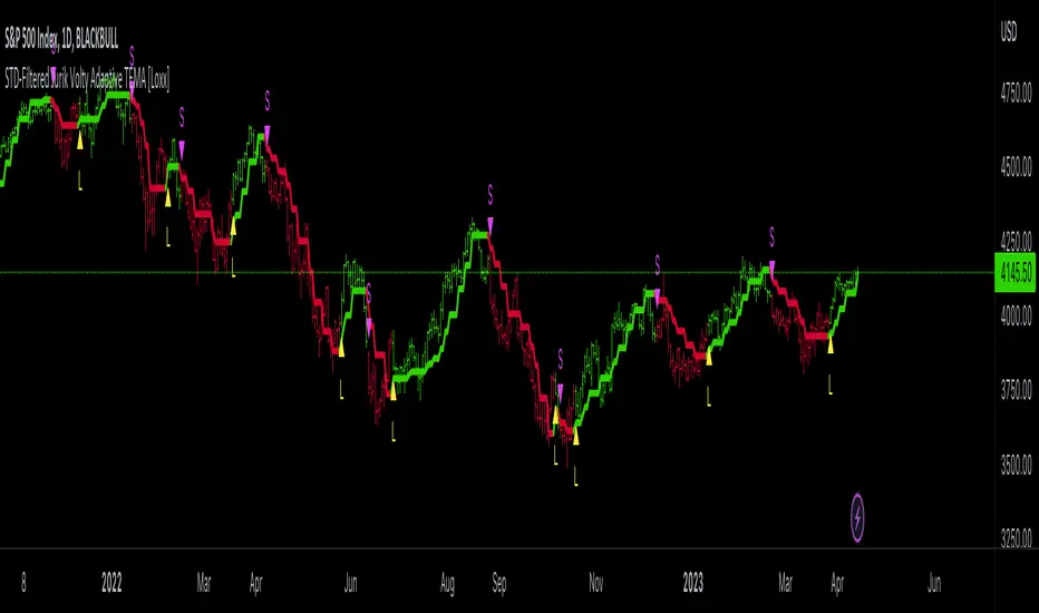
STD-Filtered Jurik Volty Adaptive TEMA [Loxx]The STD-Filtered Jurik Volty Adaptive TEMA is an advanced moving average overlay indicator that incorporates adaptive period inputs from Jurik Volty into a Triple Exponential Moving Average (TEMA). The resulting value is further refined using a standard deviation filter to minimize noise. This adaptation aims to develop a faster TEMA that leads the standard, non-adaptive TEMA. However, during periods of low volatility, the output may be noisy, so a standard deviation filter is employed to decrease choppiness, yielding a highly responsive TEMA without the noise typically caused by low market volatility.
█ What is Jurik Volty?
Jurik Volty calculates the price volatility and relative price volatility factor.
The Jurik smoothing includes 3 stages:
1st stage - Preliminary smoothing by adaptive EMA
2nd stage - One more preliminary smoothing by Kalman filter
3rd stage - Final smoothing by unique Jurik adaptive filter
Here's a breakdown of the code:
1. volty(float src, int len) => defines a function called volty that takes two arguments: src, which represents the source price data (like close price), and len, which represents the length or period for calculating the indicator.
2. int avgLen = 65 sets the length for the Simple Moving Average (SMA) to 65.
3. Various variables are initialized like volty, voltya, bsmax, bsmin, and vsum.
4. len1 is calculated as math.max(math.log(math.sqrt(0.5 * (len-1))) / math.log(2.0) + 2.0, 0); this expression involves some mathematical transformations based on the len input. The purpose is to create a dynamic factor that will be used later in the calculations.
5. pow1 is calculated as math.max(len1 - 2.0, 0.5); this variable is another dynamic factor used in further calculations.
6. del1 and del2 represent the differences between the current src value and the previous values of bsmax and bsmin, respectively.
7. volty is assigned a value based on a conditional expression, which checks whether the absolute value of del1 is greater than the absolute value of del2. This step is essential for determining the direction and magnitude of the price change.
8. vsum is updated based on the previous value and the difference between the current and previous volty values.
9. The Simple Moving Average (SMA) of vsum is calculated with the length avgLen and assigned to avg.
10. Variables dVolty, pow2, len2, and Kv are calculated using various mathematical transformations based on previously calculated variables. These variables are used to adjust the Jurik Volty indicator based on the observed volatility.
11. The bsmax and bsmin variables are updated based on the calculated Kv value and the direction of the price change.
12. inally, the temp variable is calculated as the ratio of avolty to vsum. This value represents the Jurik Volty indicator's output and can be used to analyze the market trends and potential reversals.
Jurik Volty can be used to identify periods of high or low volatility and to spot potential trade setups based on price behavior near the volatility bands.
█ What is the Triple Exponential Moving Average?
The Triple Exponential Moving Average (TEMA) is a technical indicator used by traders and investors to identify trends and price reversals in financial markets. It is a more advanced and responsive version of the Exponential Moving Average (EMA). TEMA was developed by Patrick Mulloy and introduced in the January 1994 issue of Technical Analysis of Stocks & Commodities magazine. The aim of TEMA is to minimize the lag associated with single and double exponential moving averages while also filtering out market noise, thus providing a smoother, more accurate representation of the market trend.
To understand TEMA, let's first briefly review the EMA.
Exponential Moving Average (EMA):
EMA is a weighted moving average that gives more importance to recent price data. The formula for EMA is:
EMA_t = (Price_t * α) + (EMA_(t-1) * (1 - α))
Where:
EMA_t: EMA at time t
Price_t: Price at time t
α: Smoothing factor (α = 2 / (N + 1))
N: Length of the moving average period
EMA_(t-1): EMA at time t-1
Triple Exponential Moving Average (TEMA):
Triple Exponential Moving Average (TEMA):
TEMA combines three exponential moving averages to provide a more accurate and responsive trend indicator. The formula for TEMA is:
TEMA = 3 * EMA_1 - 3 * EMA_2 + EMA_3
Where:
EMA_1: The first EMA of the price data
EMA_2: The EMA of EMA_1
EMA_3: The EMA of EMA_2
Here are the steps to calculate TEMA:
1. Choose the length of the moving average period (N).
2. Calculate the smoothing factor α (α = 2 / (N + 1)).
3. Calculate the first EMA (EMA_1) using the price data and the smoothing factor α.
4. Calculate the second EMA (EMA_2) using the values of EMA_1 and the same smoothing factor α.
5. Calculate the third EMA (EMA_3) using the values of EMA_2 and the same smoothing factor α.
5. Finally, compute the TEMA using the formula: TEMA = 3 * EMA_1 - 3 * EMA_2 + EMA_3
The Triple Exponential Moving Average, with its combination of three EMAs, helps to reduce the lag and filter out market noise more effectively than a single or double EMA. It is particularly useful for short-term traders who require a responsive indicator to capture rapid price changes. Keep in mind, however, that TEMA is still a lagging indicator, and as with any technical analysis tool, it should be used in conjunction with other indicators and analysis methods to make well-informed trading decisions.
Extras
Signals
Alerts
Bar coloring
Loxx's Expanded Source Types (see below):
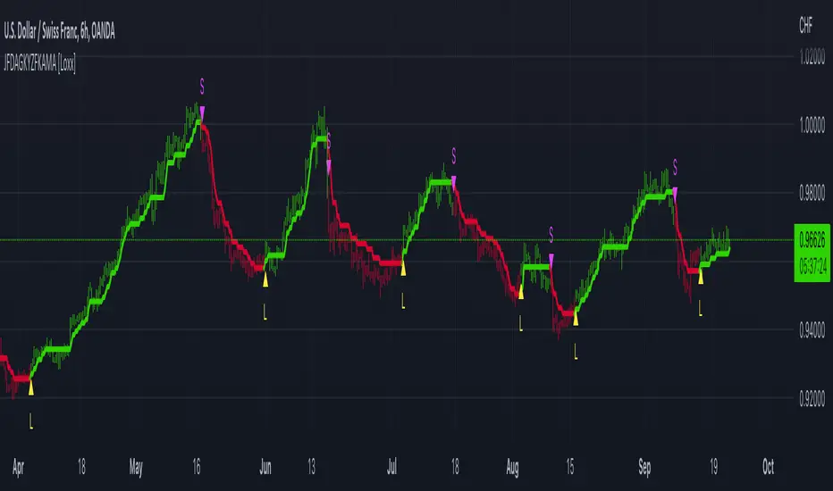
JFD-Adaptive, GKYZ-Filtered KAMA [Loxx]JFD-Adaptive, GKYZ-Filtered KAMA is a Kaufman Adaptive Moving Average with the option to make it Jurik Fractal Dimension Adaptive. This also includes a Garman-Klass-Yang-Zhang Historical Volatility Filter to reduce noise.
What is KAMA?
Developed by Perry Kaufman, Kaufman's Adaptive Moving Average ( KAMA ) is a moving average designed to account for market noise or volatility . KAMA will closely follow prices when the price swings are relatively small and the noise is low. KAMA will adjust when the price swings widen and follow prices from a greater distance. This trend-following indicator can be used to identify the overall trend, time turning points and filter price movements.
What is Jurik Fractal Dimension?
There is a weak and a strong way to measure the random quality of a time series.
The weak way is to use the random walk index ( RWI ). You can download it from the Omega web site. It makes the assumption that the market is moving randomly with an average distance D per move and proposes an amount the market should have changed over N bars of time. If the market has traveled less, then the action is considered random, otherwise it's considered trending.
The problem with this method is that taking the average distance is valid for a Normal (Gaussian) distribution of price activity. However, price action is rarely Normal, with large price jumps occuring much more frequently than a Normal distribution would expect. Consequently, big jumps throw the RWI way off, producing invalid results.
The strong way is to not make any assumption regarding the distribution of price changes and, instead, measure the fractal dimension of the time series. Fractal Dimension requires a lot of data to be accurate. If you are trading 30 minute bars, use a multi-chart where this indicator is running on 5 minute bars and you are trading on 30 minute bars.
What is Garman-Klass-Yang-Zhang Historical Volatility?
Yang and Zhang derived an extension to the Garman Klass historical volatility estimator that allows for opening jumps. It assumes Brownian motion with zero drift. This is currently the preferred version of open-high-low-close volatility estimator for zero drift and has an efficiency of 8 times the classic close-to-close estimator. Note that when the drift is nonzero, but instead relative large to the volatility , this estimator will tend to overestimate the volatility . The Garman-Klass-Yang-Zhang Historical Volatility calculation is as follows:
GKYZHV = sqrt((Z/n) * sum((log(open(k)/close( k-1 )))^2 + (0.5*(log(high(k)/low(k)))^2) - (2*log(2) - 1)*(log(close(k)/open(2:end)))^2))
Included
Alerts
Signals
Loxx's Expanded Source Types
Bar coloring
Softmax Normalized Jurik Filter Histogram [Loxx]Softmax Normalized Jurik Filter Histogram is a Jurik Filter that is morphed into a normalized oscillator from -1 to 1.
What is the Softmax function?
The softmax function, also known as softargmax: or normalized exponential function, converts a vector of K real numbers into a probability distribution of K possible outcomes. It is a generalization of the logistic function to multiple dimensions, and used in multinomial logistic regression. The softmax function is often used as the last activation function of a neural network to normalize the output of a network to a probability distribution over predicted output classes, based on Luce's choice axiom.
What is Jurik Volty used in the Juirk Filter?
One of the lesser known qualities of Juirk smoothing is that the Jurik smoothing process is adaptive. "Jurik Volty" (a sort of market volatility ) is what makes Jurik smoothing adaptive. The Jurik Volty calculation can be used as both a standalone indicator and to smooth other indicators that you wish to make adaptive.
What is the Jurik Moving Average?
Have you noticed how moving averages add some lag (delay) to your signals? ... especially when price gaps up or down in a big move, and you are waiting for your moving average to catch up? Wait no more! JMA eliminates this problem forever and gives you the best of both worlds: low lag and smooth lines.
Included:
Bar coloring
Signals
Alerts
Loxx's Expanded Source Types

FDI-Adaptive, Jurik-Filtered, TMA w/ Price Zones [Loxx]FDI-Adaptive, Jurik-Filtered, TMA w/ Price Zones is a Triangular Moving Average that is Fractal Dimension Index Adaptive with Jurik Smoothing. You'll notice that this combination not only smooths out the signal but also catches bottoms better than other FIR digital filters. This is a multi-layered adaptive moving average. Price zones are calculated using a weighted range function. Future updates will included signals associated with these range bands. For now, however, these range bands serve as support and resistance, stop-loss or take profit, or indicators of market reversal.
What is the Triangular Moving Average
The Triangular Moving Average is basically a double-smoothed Simple Moving Average that gives more weight to the middle section of the data interval. The TMA has a significant lag to current prices and is not well-suited to fast moving markets. TMA = SUM ( SMA values)/ N Where N = the number of periods.
What is the Fractal Dimension Index?
The goal of the fractal dimension index is to determine whether the market is trending or in a trading range. It does not measure the direction of the trend. A value less than 1.5 indicates that the price series is persistent or that the market is trending. Lower values of the FDI indicate a stronger trend. A value greater than 1.5 indicates that the market is in a trading range and is acting in a more random fashion.
What is Jurik Volty used in the Juirk Filter?
One of the lesser known qualities of Juirk smoothing is that the Jurik smoothing process is adaptive. "Jurik Volty" (a sort of market volatility ) is what makes Jurik smoothing adaptive. The Jurik Volty calculation can be used as both a standalone indicator and to smooth other indicators that you wish to make adaptive.
What is the Jurik Moving Average?
Have you noticed how moving averages add some lag (delay) to your signals? ... especially when price gaps up or down in a big move, and you are waiting for your moving average to catch up? Wait no more! JMA eliminates this problem forever and gives you the best of both worlds: low lag and smooth lines.
Included:
Bar coloring
Signals
Alerts
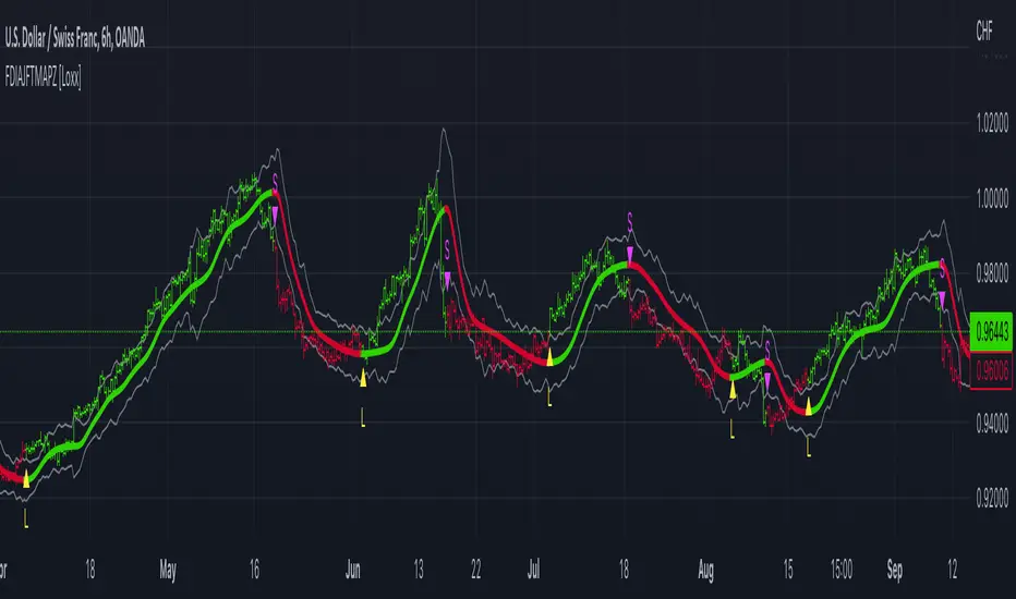
CFB-Adaptive Trend Cipher Candles [Loxx]CFB-Adaptive Trend Cipher Candles is a candle coloring indicator that shows both trend and trend exhaustion using Composite Fractal Behavior price trend analysis. To do this, we first calculate the dynamic period outputs from the CFB algorithm and then we injection those period inputs into a correlation function that correlates price input price to the candle index. The closer the correlation is to 1, the lighter the green color until the color turns yellow, sometimes, indicating upward price exhaustion. The closer the correlation is to -1, the lighter the red color until it reaches Fuchsia color indicating downward price exhaustion. Green means uptrend, red means downtrend, yellow means reversal from uptrend to downtrend, fuchsia means reversal from downtrend to uptrend.
What is Composite Fractal Behavior ( CFB )?
All around you mechanisms adjust themselves to their environment. From simple thermostats that react to air temperature to computer chips in modern cars that respond to changes in engine temperature, r.p.m.'s, torque, and throttle position. It was only a matter of time before fast desktop computers applied the mathematics of self-adjustment to systems that trade the financial markets.
Unlike basic systems with fixed formulas, an adaptive system adjusts its own equations. For example, start with a basic channel breakout system that uses the highest closing price of the last N bars as a threshold for detecting breakouts on the up side. An adaptive and improved version of this system would adjust N according to market conditions, such as momentum, price volatility or acceleration.
Since many systems are based directly or indirectly on cycles, another useful measure of market condition is the periodic length of a price chart's dominant cycle, (DC), that cycle with the greatest influence on price action.
The utility of this new DC measure was noted by author Murray Ruggiero in the January '96 issue of Futures Magazine. In it. Mr. Ruggiero used it to adaptive adjust the value of N in a channel breakout system. He then simulated trading 15 years of D-Mark futures in order to compare its performance to a similar system that had a fixed optimal value of N. The adaptive version produced 20% more profit!
This DC index utilized the popular MESA algorithm (a formulation by John Ehlers adapted from Burg's maximum entropy algorithm, MEM). Unfortunately, the DC approach is problematic when the market has no real dominant cycle momentum, because the mathematics will produce a value whether or not one actually exists! Therefore, we developed a proprietary indicator that does not presuppose the presence of market cycles. It's called CFB (Composite Fractal Behavior) and it works well whether or not the market is cyclic.
CFB examines price action for a particular fractal pattern, categorizes them by size, and then outputs a composite fractal size index. This index is smooth, timely and accurate
Essentially, CFB reveals the length of the market's trending action time frame. Long trending activity produces a large CFB index and short choppy action produces a small index value. Investors have found many applications for CFB which involve scaling other existing technical indicators adaptively, on a bar-to-bar basis.
Included
Loxx's Expanded Source Types
Related indicators:
Adaptive Trend Cipher loxx]
Dynamic Zones Polychromatic Momentum Candles
RSI Precision Trend Candles
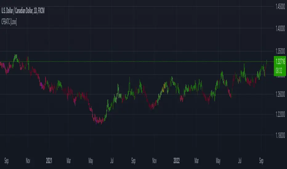
TDI w/ Variety RSI, Averages, & Source Types [Loxx]This hybrid indicator is developed to assist traders in their ability to decipher and monitor market conditions related to trend direction, market strength, and market volatility. Even though comprehensive, the Traders Dynamic Index (TDI) is easy to read and use. This version of TDI has 7 different types of RSI, 38 different types of Moving Averages, 33 source types, and 5 types of signals as well as alerts and coloring. Default RSI type is set to Jurik's RSX. This indicator can be used on any timeframe.
Green/Red line = RSI Price line
White line = Trade Signal line
Dark Green/Red lines = Volatility Band
Yellow line = Market Base Line
Gray dashed lines = Horizontal boundary lines, oversold/overbought
5 Signal Types w/ Alerts
Signal Crosses = Green/Red line crosses over or under White line
Floating Boundary Crosses = Green/Red line crosses over or under upper Dark Green/ lower Red lines
Horizontal Boundary Crosses = Green/Red line crosses over or under Gray dashed upper/lower lines
Floating Middle Crosses = Green/Red line crosses over or under Yellow line
Horizontal Middle Crosses = Green/Red line crosses over or under Gray dashed middle line
Manual Signal Types (no alerts included, this requires manual analysis)
Volatility Band Signals (Dark Green/Red lines) = When the Dark Green/Red lines are expanding, the market is strong and trending. When Dark Green/Red lines are constricting, the market is weak and in a range. When the Dark Green/Red lines are extremely tight in a narrow range, expect an economic announcement or other market condition to spike the market
Beyond these simple signal rules, there are various other signals or methods that can be used to derive long/short/exit signals from TDI included slope of the Green/Red line and bounces off the Yellow line.
Included
Loxx's Expanded Source Types
Loxx's Variety RSI
Loxx's Moving Averages
Signals
Alerts
Bar coloring
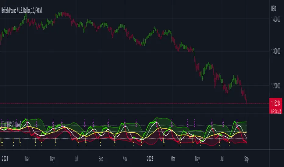
Jurik-Filtered Kase Permission Stochastic [Loxx]Jurik-Filtered Kase Permission Stochastic is a special implementation of Kase Permission Stochastic by Kase StatWare. This implementation uses a Jurik filter to smooth final output.
What is Kase StatWare?
Kase StatWare has been around since 1992 and is a technical analysis trading indicator package developed by the acclaimed market technician and former energy trader Cynthia A. Kase. StatWare’s self-optimizing indicators help professional and individual traders to form a precise and systematic approach to discretionary trading and trade risk management.
Kase StatWare creates subscription-based technical analysis tools mainly for Stocks and Futures trading which can be subscribed to at a monthly cost.
What is Kase Permission Stochastic?
The Kase Permission Stochastic is a momentum indicator that examines a synthetic longer bar length, that by default, is three (5x by default for this implementation here) times higher than the bar length it is plotted against.
Included
Alerts
Signals
Bar coloring
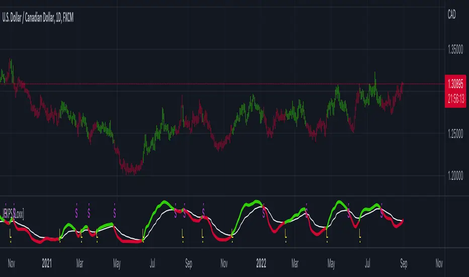
CFB-Adaptive, Jurik DMX Histogram [Loxx]Jurik DMX Histogram is the ultra-smooth, low lag version of your classic DMI indicator. This is a momentum indicator. You can use this indicator standalone or as part of a system with a moving average and a mean reversion indicator. This indicator has both composite fractal behavior adaptive inputs and fixed inputs. The default is CFB adaptive. Dark green means strong push up, dark red, strong push down. Light green means weak push up, and light red means weak push down.
What is the directional movement index?
The directional movement index (DMI) is an indicator developed by J. Welles Wilder in 1978 that identifies in which direction the price of an asset is moving. The indicator does this by comparing prior highs and lows and drawing two lines: a positive directional movement line ( +DI ) and a negative directional movement line ( -DI ). An optional third line, called the average directional index ( ADX ), can also be used to gauge the strength of the uptrend or downtrend.
When +DI is above -DI , there is more upward pressure than downward pressure in the price. Conversely, if -DI is above +DI , then there is more downward pressure on the price. This indicator may help traders assess the trend direction. Crossovers between the lines are also sometimes used as trade signals to buy or sell.
What is Composite Fractal Behavior ( CFB )?
All around you mechanisms adjust themselves to their environment. From simple thermostats that react to air temperature to computer chips in modern cars that respond to changes in engine temperature, r.p.m.'s, torque, and throttle position. It was only a matter of time before fast desktop computers applied the mathematics of self-adjustment to systems that trade the financial markets.
Unlike basic systems with fixed formulas, an adaptive system adjusts its own equations. For example, start with a basic channel breakout system that uses the highest closing price of the last N bars as a threshold for detecting breakouts on the up side. An adaptive and improved version of this system would adjust N according to market conditions, such as momentum, price volatility or acceleration.
Since many systems are based directly or indirectly on cycles, another useful measure of market condition is the periodic length of a price chart's dominant cycle, (DC), that cycle with the greatest influence on price action.
The utility of this new DC measure was noted by author Murray Ruggiero in the January '96 issue of Futures Magazine. In it. Mr. Ruggiero used it to adaptive adjust the value of N in a channel breakout system. He then simulated trading 15 years of D-Mark futures in order to compare its performance to a similar system that had a fixed optimal value of N. The adaptive version produced 20% more profit!
This DC index utilized the popular MESA algorithm (a formulation by John Ehlers adapted from Burg's maximum entropy algorithm, MEM). Unfortunately, the DC approach is problematic when the market has no real dominant cycle momentum, because the mathematics will produce a value whether or not one actually exists! Therefore, we developed a proprietary indicator that does not presuppose the presence of market cycles. It's called CFB (Composite Fractal Behavior) and it works well whether or not the market is cyclic.
CFB examines price action for a particular fractal pattern, categorizes them by size, and then outputs a composite fractal size index. This index is smooth, timely and accurate
Essentially, CFB reveals the length of the market's trending action time frame. Long trending activity produces a large CFB index and short choppy action produces a small index value. Investors have found many applications for CFB which involve scaling other existing technical indicators adaptively, on a bar-to-bar basis.
What is Jurik Volty used in the Juirk Filter?
One of the lesser known qualities of Juirk smoothing is that the Jurik smoothing process is adaptive. "Jurik Volty" (a sort of market volatility ) is what makes Jurik smoothing adaptive. The Jurik Volty calculation can be used as both a standalone indicator and to smooth other indicators that you wish to make adaptive.
What is the Jurik Moving Average?
Have you noticed how moving averages add some lag (delay) to your signals? ... especially when price gaps up or down in a big move, and you are waiting for your moving average to catch up? Wait no more! JMA eliminates this problem forever and gives you the best of both worlds: low lag and smooth lines.
Ideally, you would like a filtered signal to be both smooth and lag-free. Lag causes delays in your trades, and increasing lag in your indicators typically result in lower profits. In other words, late comers get what's left on the table after the feast has already begun.
Included:
Alerts
Loxx's Expanded Source Types
Signals
Bar coloring

Juirk-Filtered QQE Histogram [Loxx]Juirk-Filtered QQE Histogram is a QQE indicator with 7 different RSI types, Jurik-Filtering with the option of double filtering. 2 types of signals, and Loxx's Expanded Source types. These additions are useful to filter out noise.
What is Qualitative Quantitative Estimation (QQE)?
The Qualitative Quantitative Estimation (QQE) indicator works like a smoother version of the popular Relative Strength Index ( RSI ) indicator. QQE expands on RSI by adding two volatility based trailing stop lines. These trailing stop lines are composed of a fast and a slow moving Average True Range (ATR).
There are many indicators for many purposes. Some of them are complex and some are comparatively easy to handle. The QQE indicator is a really useful analytical tool and one of the most accurate indicators. It offers numerous strategies for using the buy and sell signals. Essentially, it can help detect trend reversal and enter the trade at the most optimal positions.
What is Jurik Volty used in the Juirk Filter?
One of the lesser known qualities of Juirk smoothing is that the Jurik smoothing process is adaptive. "Jurik Volty" (a sort of market volatility ) is what makes Jurik smoothing adaptive. The Jurik Volty calculation can be used as both a standalone indicator and to smooth other indicators that you wish to make adaptive.
What is the Jurik Moving Average?
Have you noticed how moving averages add some lag (delay) to your signals? ... especially when price gaps up or down in a big move, and you are waiting for your moving average to catch up? Wait no more! JMA eliminates this problem forever and gives you the best of both worlds: low lag and smooth lines.
Ideally, you would like a filtered signal to be both smooth and lag-free. Lag causes delays in your trades, and increasing lag in your indicators typically result in lower profits. In other words, late comers get what's left on the table after the feast has already begun.
Included:
Loxx's Expanded Source Types
Alerts
Signals
Bar coloring
Included Libraries
Loxx's Variety RSI
Loxx's Jurik Tools
Loxx's Expanded Source Types
Related indicators:
Natural Market Mirror (NMM) and NMAs w/ Dynamic Zones
RSI/RSX QQE Histogram w/ Discontinued Signal Line
Jurik CFB Adaptive QQE
Adaptive Qualitative Quantitative Estimation (QQE)
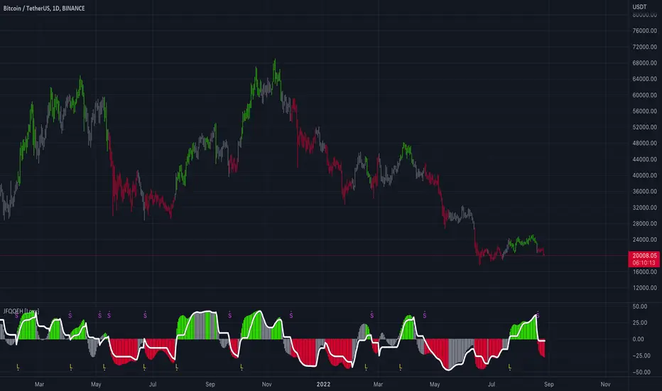
Variety RSI of Fast Discrete Cosine Transform [Loxx]Variety RSI of Fast Discrete Cosine Transform is an RSI indicator with 7 types of RSI that is calculated on the Fast Discrete Cosine Transform of source. The source inputs are 33 different source types from Loxx's Expanded Source Types.
What is Discrete Cosine Transform?
A discrete cosine transform (DCT) expresses a finite sequence of data points in terms of a sum of cosine functions oscillating at different frequencies. The DCT, first proposed by Nasir Ahmed in 1972, is a widely used transformation technique in signal processing and data compression. It is used in most digital media, including digital images (such as JPEG and HEIF, where small high-frequency components can be discarded), digital video (such as MPEG and H.26x), digital audio (such as Dolby Digital, MP3 and AAC), digital television (such as SDTV, HDTV and VOD), digital radio (such as AAC+ and DAB+), and speech coding (such as AAC-LD, Siren and Opus). DCTs are also important to numerous other applications in science and engineering, such as digital signal processing, telecommunication devices, reducing network bandwidth usage, and spectral methods for the numerical solution of partial differential equations.
Fast Discrete Cosine Transform
The algorithm performs a fast cosine transform of the real function defined by nn samples on the real axis.
Depending on the passed parameters, it can be executed both direct and inverse conversion.
Input parameters:
tnn - Number of function values minus one. Should be 1024 degree of two. The algorithm does not check correct value passed.
a - array of Real 1025 Function values.
InverseFCT - the direction of the transformation. True if reverse, False if direct.
Output parameters: a - the result of the transformation. For more details, see description on the site. www.alglib.net
Included:
7 types of RSI
33 source inputs from Loxx's Expanded Source Types
2 types of signals
Alerts
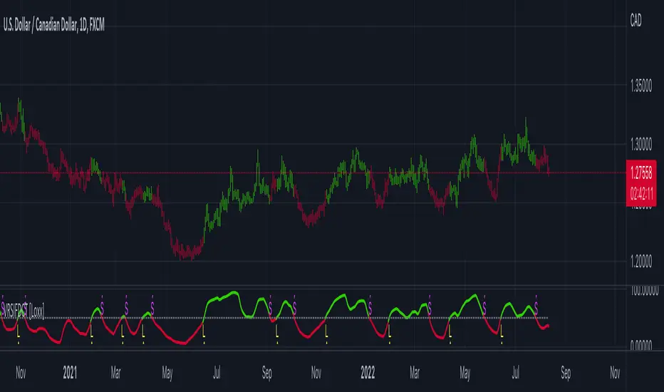
STD-Filtered Variety RSI of Double Averages w/ DSL [Loxx]STD-Filtered Variety RSI of Double Averages w/ DSL is a standard deviation step filtered RSI indicator that is calculated using double smoothing. The user can choose from 8 different RSI types and 38 different double smoothing types. This indicator uses Discontinued Signal Lines instead of regular signals and levels. This allows the signals to be more precise in catching early trend breakouts and breakdowns.
Things to note
Double smoothing of the source does not function like DEMA, for example. This double smoothing is just smoothing of smoothing of source
There are two types of smoothing for Discontinued Signals Lines: Regular EMA and Fast EMA
T3 RSI has been added on top of Loxx's Variety RSI library
Contained inside this indicator
Loxx's Moving Averages
Loxx's Variety RSI
Related indicators
Corrected RSI w/ Floating Levels
Adaptive, Jurik-Filtered, Floating RSI
Variety RSI w/ Dynamic Zones
Included
Bar coloring
Alerts
2 types of signals with precision adjustment
Loxx's Variety RSI
Loxx's Moving Averages

Jurik Smoothed Stochastic - TraderHalaiJurik Smoothed Stochastic
The stochastic indicator has been long used by traders to identify inflection points in the price and to give a direction on Bullish and Bearish bias.
This indicator aims to improve on the plots the %K value smoothed using a Jurik Filter instead of a simple moving average. This allows for a more adaptive K value average price, whilst also providing superior smoothing to traditional moving averages.
As the Jurik Filter is a proprietary and non-open-source implementation, this script uses a common filters library implementation of Jurik MA which is a suitable proxy to the actual Jurik MA filter.
Big thanks to LastGuru for making his version freely available. You can find his version of the Jurik Filters in the credits section below.
%K is the Jurik Smoothed Version of the original Stochastic Formula
%D is calculated using the following formula. This idea was borrowed from John Ehler’s stochastic implementation and can be seen below:
%D = 0.05 + 0.95 * K
Features
%K line, Overbought and Oversold level and Mid Line Level
Oversold / Overbought reversal indicators and signals - Shown in Red and Green
Bullish / Bearish Divergences – Including Hidden divergences to spot reversals and continuations of trend (Big thanks to the developers of the built-in RSI Divergence indicator) - Shown as below:
Bullish / Bearish crossover of %K with %D - Shown in Cyan and Fuschia
Alerts for all of the above conditions
Double Jurik smoothing mode - similar to slow Stochastic
Credits :
Massive shoutout to the following scripts:
LastGuru JurikMA implementation (Common Filters Library)
Divergence Indicator – Built into TradingView and coded by TradingView Developers
This script is published as open source to allow for criticism, further development of this strategy and use by the community. Feel free to use this indicator/source code as you see fit.
Enjoy! :)

Fourier Extrapolator of Variety RSI w/ Bollinger Bands [Loxx]Fourier Extrapolator of Variety RSI w/ Bollinger Bands is an RSI indicator that shows the original RSI, the Fourier Extrapolation of RSI in the past, and then the projection of the Fourier Extrapolated RSI for the future. This indicator has 8 different types of RSI including a new type of RSI called T3 RSI. The purpose of this indicator is to demonstrate the Fourier Extrapolation method used to model past data and to predict future price movements. This indicator will repaint. If you wish to use this for trading, then make sure to take a screenshot of the indicator when you enter the trade to save your analysis. This is the first of a series of forecasting indicators that can be used in trading. Due to how this indicator draws on the screen, you must choose values of npast and nfut that are equal to or less than 200. this is due to restrictions by TradingView and Pine Script in only allowing 500 lines on the screen at a time. Enjoy!
What is Fourier Extrapolation?
This indicator uses a multi-harmonic (or multi-tone) trigonometric model of a price series xi, i=1..n, is given by:
xi = m + Sum( a*Cos(w*i) + b*Sin(w*i), h=1..H )
Where:
xi - past price at i-th bar, total n past prices;
m - bias;
a and b - scaling coefficients of harmonics;
w - frequency of a harmonic ;
h - harmonic number;
H - total number of fitted harmonics.
Fitting this model means finding m, a, b, and w that make the modeled values to be close to real values. Finding the harmonic frequencies w is the most difficult part of fitting a trigonometric model. In the case of a Fourier series, these frequencies are set at 2*pi*h/n. But, the Fourier series extrapolation means simply repeating the n past prices into the future.
This indicator uses the Quinn-Fernandes algorithm to find the harmonic frequencies. It fits harmonics of the trigonometric series one by one until the specified total number of harmonics H is reached. After fitting a new harmonic , the coded algorithm computes the residue between the updated model and the real values and fits a new harmonic to the residue.
see here: A Fast Efficient Technique for the Estimation of Frequency , B. G. Quinn and J. M. Fernandes, Biometrika, Vol. 78, No. 3 (Sep., 1991), pp . 489-497 (9 pages) Published By: Oxford University Press
The indicator has the following input parameters:
src - input source
npast - number of past bars, to which trigonometric series is fitted;
Nfut - number of predicted future bars;
nharm - total number of harmonics in model;
frqtol - tolerance of frequency calculations.
Included:
Loxx's Expanded Source Types
Loxx's Variety RSI
Other indicators using this same method
Fourier Extrapolator of Price w/ Projection Forecast
Fourier Extrapolator of Price
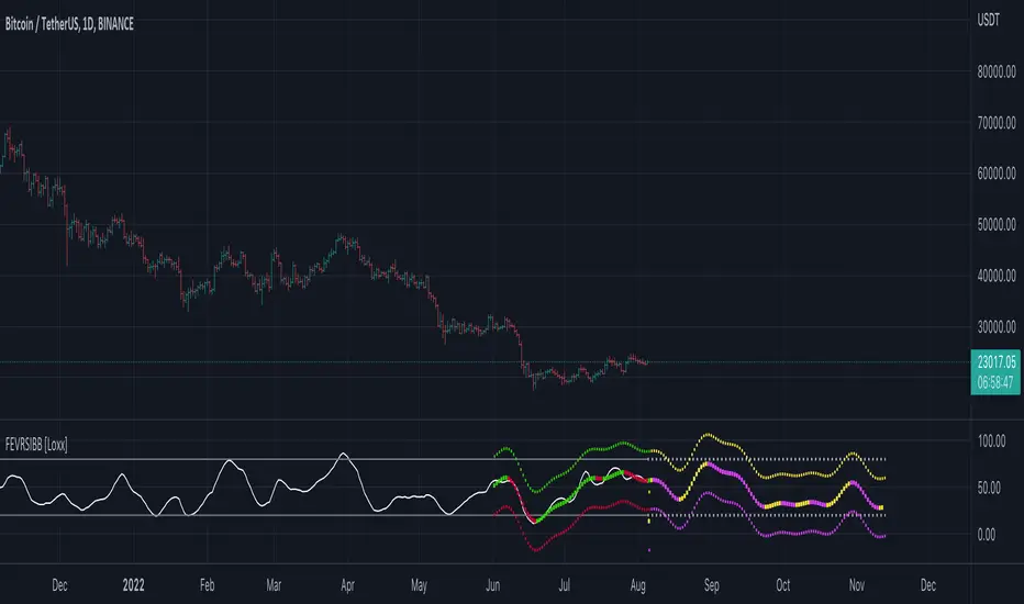
VHF-Adaptive, Digital Kahler Variety RSI w/ Dynamic Zones [Loxx]VHF-Adaptive, Digital Kahler Variety RSI w/ Dynamic Zones is an RSI indicator with adaptive inputs, Digital Kahler filtering, and Dynamic Zones. This indicator uses a Vertical Horizontal Filter for calculating the adaptive period inputs and allows the user to select from 7 different types of RSI.
What is VHF Adaptive Cycle?
Vertical Horizontal Filter (VHF) was created by Adam White to identify trending and ranging markets. VHF measures the level of trend activity, similar to ADX DI. Vertical Horizontal Filter does not, itself, generate trading signals, but determines whether signals are taken from trend or momentum indicators. Using this trend information, one is then able to derive an average cycle length.
What is Digital Kahler?
From Philipp Kahler's article for www.traders-mag.com, August 2008. "A Classic Indicator in a New Suit: Digital Stochastic"
Digital Indicators
Whenever you study the development of trading systems in particular, you will be struck in an extremely unpleasant way by the seemingly unmotivated indentations and changes in direction of each indicator. An experienced trader can recognise many false signals of the indicator on the basis of his solid background; a stupid trading system usually falls into any trap offered by the unclear indicator course. This is what motivated me to improve even further this and other indicators with the help of a relatively simple procedure. The goal of this development is to be able to use this indicator in a trading system with as few additional conditions as possible. Discretionary traders will likewise be happy about this clear course, which is not nerve-racking and makes concentrating on the essential elements of trading possible.
How Is It Done?
The digital stochastic is a child of the original indicator. We owe a debt of gratitude to George Lane for his idea to design an indicator which describes the position of the current price within the high-low range of the historical price movement. My contribution to this indicator is the changed pattern which improves the quality of the signal without generating too long delays in giving signals. The trick used to generate this “digital” behavior of the indicator. It can be used with most oscillators like RSI or CCI .
First of all, the original is looked at. The indicator always moves between 0 and 100. The precise position of the indicator or its course relative to the trigger line are of no interest to me, I would just like to know whether the indicator is quoted below or above the value 50. This is tantamount to the question of whether the market is just trading above or below the middle of the high-low range of the past few days. If the market trades in the upper half of its high-low range, then the digital stochastic is given the value 1; if the original stochastic is below 50, then the value –1 is given. This leads to a sequence of 1/-1 values – the digital core of the new indicator. These values are subsequently smoothed by means of a short exponential moving average . This way minor false signals are eliminated and the indicator is given its typical form.
What are Dynamic Zones?
As explained in "Stocks & Commodities V15:7 (306-310): Dynamic Zones by Leo Zamansky, Ph .D., and David Stendahl"
Most indicators use a fixed zone for buy and sell signals. Here’ s a concept based on zones that are responsive to past levels of the indicator.
One approach to active investing employs the use of oscillators to exploit tradable market trends. This investing style follows a very simple form of logic: Enter the market only when an oscillator has moved far above or below traditional trading lev- els. However, these oscillator- driven systems lack the ability to evolve with the market because they use fixed buy and sell zones. Traders typically use one set of buy and sell zones for a bull market and substantially different zones for a bear market. And therein lies the problem.
Once traders begin introducing their market opinions into trading equations, by changing the zones, they negate the system’s mechanical nature. The objective is to have a system automatically define its own buy and sell zones and thereby profitably trade in any market — bull or bear. Dynamic zones offer a solution to the problem of fixed buy and sell zones for any oscillator-driven system.
An indicator’s extreme levels can be quantified using statistical methods. These extreme levels are calculated for a certain period and serve as the buy and sell zones for a trading system. The repetition of this statistical process for every value of the indicator creates values that become the dynamic zones. The zones are calculated in such a way that the probability of the indicator value rising above, or falling below, the dynamic zones is equal to a given probability input set by the trader.
To better understand dynamic zones, let's first describe them mathematically and then explain their use. The dynamic zones definition:
Find V such that:
For dynamic zone buy: P{X <= V}=P1
For dynamic zone sell: P{X >= V}=P2
where P1 and P2 are the probabilities set by the trader, X is the value of the indicator for the selected period and V represents the value of the dynamic zone.
The probability input P1 and P2 can be adjusted by the trader to encompass as much or as little data as the trader would like. The smaller the probability, the fewer data values above and below the dynamic zones. This translates into a wider range between the buy and sell zones. If a 10% probability is used for P1 and P2, only those data values that make up the top 10% and bottom 10% for an indicator are used in the construction of the zones. Of the values, 80% will fall between the two extreme levels. Because dynamic zone levels are penetrated so infrequently, when this happens, traders know that the market has truly moved into overbought or oversold territory.
Calculating the Dynamic Zones
The algorithm for the dynamic zones is a series of steps. First, decide the value of the lookback period t. Next, decide the value of the probability Pbuy for buy zone and value of the probability Psell for the sell zone.
For i=1, to the last lookback period, build the distribution f(x) of the price during the lookback period i. Then find the value Vi1 such that the probability of the price less than or equal to Vi1 during the lookback period i is equal to Pbuy. Find the value Vi2 such that the probability of the price greater or equal to Vi2 during the lookback period i is equal to Psell. The sequence of Vi1 for all periods gives the buy zone. The sequence of Vi2 for all periods gives the sell zone.
In the algorithm description, we have: Build the distribution f(x) of the price during the lookback period i. The distribution here is empirical namely, how many times a given value of x appeared during the lookback period. The problem is to find such x that the probability of a price being greater or equal to x will be equal to a probability selected by the user. Probability is the area under the distribution curve. The task is to find such value of x that the area under the distribution curve to the right of x will be equal to the probability selected by the user. That x is the dynamic zone.
Included:
Bar coloring
4 signal types
Alerts
Loxx's Expanded Source Types
Loxx's Moving Averages
Loxx's Variety RSI
Loxx's Dynamic Zones

Adaptive-Lookback CCI w/ Double Juirk Smoothing [Loxx]Adaptive-Lookback CCI w/ Double Juirk Smoothing is a CCI indicator with Adaptive period inputs. The adaptive calculation in this case is the count of pivots in historical bars. This indicator is also double smoothing using Jurik smoothing to reduce noise and refine the signal.
What is CCI?
The Commodity Channel Index ( CCI ) measures the current price level relative to an average price level over a given period of time. CCI is relatively high when prices are far above their average. CCI is relatively low when prices are far below their average. Using this method, CCI can be used to identify overbought and oversold levels.
What is Jurik Volty used in the Juirk Filter?
One of the lesser known qualities of Juirk smoothing is that the Jurik smoothing process is adaptive. "Jurik Volty" (a sort of market volatility ) is what makes Jurik smoothing adaptive. The Jurik Volty calculation can be used as both a standalone indicator and to smooth other indicators that you wish to make adaptive.
What is the Jurik Moving Average?
Have you noticed how moving averages add some lag (delay) to your signals? ... especially when price gaps up or down in a big move, and you are waiting for your moving average to catch up? Wait no more! JMA eliminates this problem forever and gives you the best of both worlds: low lag and smooth lines.
Included:
Bar coloring
3 signal variations w/ alerts

True Adaptive-Lookback Phase Change Index [Loxx]Previously I posted a Phase Change Index using Ehlers Autocorrelation Periodogram Algorithm to tease out the adaptive periods. You can find the previous version here: . This new version is also adaptive but uses a different method to derive the adaptive length inputs. This adaptive method derives period inputs by counting pivots from past candles. This version also relies on Jurik Smoothing to generate the final signal. I named this one "true" because I should have specified in the previous PCI's title that it's powered by Ehlers Autocorrelation Periodogram. Additionally, you'll notice the ALB algorithm has changed from other indicators, This is restrict the range of possible ALB period outputs to a specific range so the indicator is usable.
And remember, this is an inverse indicator. This means that small values on the oscillator indicate bullish sentiment and higher values on the oscillator indicate bearish sentiment.
What is the Phase Change Index?
Based on the M.H. Pee's TASC article "Phase Change Index".
Prices at any time can be up, down, or unchanged. A period where market prices remain relatively unchanged is referred to as a consolidation. A period that witnesses relatively higher prices is referred to as an uptrend, while a period of relatively lower prices is called a downtrend.
The Phase Change Index ( PCI ) is an indicator designed specifically to detect changes in market phases.
This indicator is made as he describes it with one deviation: if we follow his formula to the letter then the "trend" is inverted to the actual market trend. Because of that an option to display inverted (and more logical) values is added.
What is the Jurik Moving Average?
Have you noticed how moving averages add some lag (delay) to your signals? ... especially when price gaps up or down in a big move, and you are waiting for your moving average to catch up? Wait no more! JMA eliminates this problem forever and gives you the best of both worlds: low lag and smooth lines.
Ideally, you would like a filtered signal to be both smooth and lag-free. Lag causes delays in your trades, and increasing lag in your indicators typically result in lower profits. In other words, late comers get what's left on the table after the feast has already begun.
That's why investors, banks and institutions worldwide ask for the Jurik Research Moving Average ( JMA ). You may apply it just as you would any other popular moving average. However, JMA's improved timing and smoothness will astound you.
What is adaptive Jurik volatility
One of the lesser known qualities of Juirk smoothing is that the Jurik smoothing process is adaptive. "Jurik Volty" (a sort of market volatility ) is what makes Jurik smoothing adaptive. The Jurik Volty calculation can be used as both a standalone indicator and to smooth other indicators that you wish to make adaptive.
Included:
Bar coloring
2 signal variations w/ alerts
