Adaptive Multi-Method ForecastWhat This Indicator Does:
An intelligent forecasting system that predicts future price movement and provides automated TP/SL levels for trading across ALL timeframes.
📊 Core Features:
1. Adaptive Forecasting (3 Methods)
Linear Regression: Best for trending markets (Daily/Weekly)
EMA Projection: Best for fast-moving intraday (1m-1h)
Hybrid: Combines both methods for balanced approach
Auto Mode: Automatically selects the best method for your timeframe ✅
2. Visual Elements on Chart:
ElementColorWhat It ShowsForecast Line🟢 Green (bullish) / 🔴 Red (bearish) / 🟡 Yellow (neutral)Predicted price in X bars aheadLR Line (Blue)🔵 BlueLinear regression trend lineConfidence Zone🟢/🔴 Shaded area (65% visible)Probable price rangeUpper/Lower Bands🟢 Green / 🔴 Red lines (65% visible)Forecast uncertainty boundariesBUY Signal🟢 Small green triangle ▲Price crossed above trend - Long opportunitySELL Signal🔴 Small red triangle ▼Price crossed below trend - Short opportunity
3. Trade Management (TP/SL)
When BUY signal appears:
🟡 Yellow line = Entry price (where you bought)
🟢 Green line = Take Profit target (+2.5% by default)
🔴 Red line = Stop Loss (-1.5% by default)
When SELL signal appears:
🟡 Yellow line = Entry price (where you sold)
🟠 Orange line = Take Profit target (-2.5%)
🟣 Fuchsia line = Stop Loss (+1.5%)
Lines disappear when:
TP is hit ✅ (profit secured)
SL is hit ❌ (loss cut)
Ready for next signal
📱 Info Table (Top Right):
Shows real-time data:
Method: Which forecast method is active
Timeframe: Your current chart timeframe
Trend: Bullish ↑ / Bearish ↓ / Neutral →
Current: Current price
Forecast: Predicted price
Change: Expected % move
Position: LONG / SHORT / None
Entry: Your entry price (when in position)
P&L: Current profit/loss % (when in position)
⚙️ Settings You Can Adjust:
Forecast Settings:
Method: Auto (recommended) / Linear / EMA / Hybrid
Length: 20 bars (how much history to analyze)
Forecast Bars: 10 bars ahead (prediction distance)
Sensitivity: 1.0 (higher = more aggressive forecast)
Show Confidence Bands: ✅ On/Off
Trade Management:
Show TP/SL Levels: ✅ On/Off
Take Profit %: 2.5% (adjustable)
Stop Loss %: 1.5% (adjustable)
Use Forecast as TP: ❌ Off (uses fixed % instead)
🔔 Alerts Available:
BUY Signal - Bullish crossover detected
SELL Signal - Bearish crossunder detected
Long TP Hit - Take profit reached
Long SL Hit - Stop loss triggered
Short TP Hit - Take profit reached
Short SL Hit - Stop loss triggered
✅ Works On All Timeframes:
✅ Intraday: 1m, 5m, 15m, 30m, 1h (uses EMA Projection)
✅ Swing: 4h, Daily (uses Hybrid)
✅ Position: Weekly, Monthly (uses Linear Regression)
📈 How To Use:
Add to chart - Indicator loads automatically
Wait for signal - Green ▲ (BUY) or Red ▼ (SELL)
Enter trade - Yellow entry line appears
Set alerts - Get notified on TP/SL hits
Exit auto - When price hits green (TP) or red (SL) line
Repeat - Wait for next signal
⚠️ Important Notes:
Not 100% accurate - No indicator predicts perfectly
Use risk management - Always respect stop losses
Best in trends - Less accurate in sideways markets
Combine with other analysis - Support/resistance, volume, news
Backtest first - Test on historical data before live trading
🎯 Best Practices:
✅ Keep on "Auto" mode for best results
✅ Use on trending assets (stocks, crypto with clear direction)
✅ Respect all stop losses
✅ Don't override forecast with emotions
✅ Start with 10 forecast bars, adjust based on your trading style
✅ Enable all alerts for real-time notifications
線性回歸(LR)

Logit Alpha Ranker For BTCThe ORLA Ranker is a "Fat-Tail" strategy. It is designed to ignore noise and only participate in high-probability, high-conviction trends. Its ability to achieve a 3.8+ Profit Factor on BTC suggests that the Logit model effectively filters out the volatility "churn" that kills most retail trend-following scripts.
Efficiency: The strategy is highly selective, with only 66 trades over nearly a decade. This low frequency minimizes commission drag and slippage.

Auto TrendLine ProAuto TrendLine Pro is a smart, automated trendline tool designed for traders who value quality over quantity.
Most indicators draw too many lines, making the chart messy and confusing. This engine solves that by filtering out the " noise. " It hunts for mathematically precise connections between market pivots. It gives you a clean view of the strongest Support and Resistance levels that the market is actually respecting.
Menu Options Explained
Here is how you can control the indicator using the settings menu:
1. Swing Length
This setting controls the "eyes" of the engine—how it finds the Highs and Lows.
Swing Length determines how far back the engine looks.
Small numbers (1 or 2): It finds more short-term swings.
Big numbers(3 to 10): It ignores small moves and only looks for major market turns.
2. Trendline Strength
This shows how strong the trendline is. 1 is a good score for a valid trendline. If you increase this number you will get stronger trendlines.
3. Touch Threshold
How strict should the engine be?
Low value: Very strict. Price must touch the line perfectly.
High value: More relaxed. Near-misses are counted as touches.
4. Breakout Threshold
This prevents false alarms. If a candle wick pokes through the line just a little bit but closes back inside, this setting tells the engine to ignore it and keep the trendline alive.
5. Source
This controls where a trendline starts.
Wick: The line must start at the very tip of the candle's Wick (High/Low). This usually gives the most precise touches.
Body: The line starts from the candle's Body (Close). This is usually recommended for line charts.
Best Match(Recommended): The engine tries both and picks the one that fits the math better.
6. Display Mode
This controls how many lines you see on the screen.
Oldest Line: Shows only the single best Support and Resistance line.
Recent Lines: Shows the top 2 or 3 best lines.
Only Specific Line: Shows only a specific line(e.g., only the 2nd best line).
7. Lines to Display
This option controls exactly how many trendlines appear on your chart at the same time, such as showing only the single oldest line or the top 3. It helps declutter your view by hiding weaker lines so you can focus only on the most critical support and resistance levels.
Trendline Types:
1. Confirmed Trendlines
These are solid, established lines that have been tested by price enough times to be locked in as reliable barriers. Unlike live lines, they are permanent and will not disappear or move, providing a trustworthy reference for Support and Resistance.
2. Live Trendlines
These are tentative lines that have just started to form but have not been fully confirmed yet. They show you potential setups early, but they are risky because they might disappear if the price invalidates them before they become strong.
3. Broadening Trendlines
Broadening Trendlines open up wider like a Loudspeaker as they move forward, instead of squeezing together like a normal triangle.
4. Freeze on Live
This option stops the trendlines from moving or flickering while the current candle is still forming. The lines will only update once the candle finishes and closes, keeping your chart stable. Trade-off: You are sacrificing Real-time Reaction to get Stability.
Breached Trendlines, Visuals and Alerts are self Explanatory.
Future updates will have lots of other features.
⚠️ DISCLAIMER
This indicator is for educational purposes only and does not constitute financial advice. Trading involves substantial risk of loss. Past performance does not guarantee future results. Use at your own risk.
© Auto TrendLine Pro - All rights reserved. Copying, redistribution, or reverse-engineering is prohibited without written consent.

Vietnamese Stock: Discount Linear Regression Liquidity GrabThe Discount Linear Regression Liquidity Grab is a sophisticated technical analysis tool that combines statistical trend analysis with Premium/Discount Zone and Price Action logic. Unlike standard Linear Regression Channels that repaint or stretch indefinitely, this indicator is dynamic: it automatically detects volatility breakouts to "reset" the channel, creating distinct market "Sections."
This tool is designed to help traders identify trend exhaustion, fair value gaps (FVGs), and high-probability reversal or continuation zones using two distinct built-in strategies.
Key Features
1. Dynamic Channel Resets
The core engine calculates a Linear Regression Channel based on a Pearson R coefficient and Deviation multipliers.
- How it works: When price breaks out of the Upper or Lower Deviation bands, the script recognizes a shift in momentum. It "locks" the previous channel and begins calculating a new one from the breakout point.
- Benefit: This creates a historical map of market structure, showing you exactly where previous trends began and ended.
2. Smart Money Concepts (SMC) Integration
For every completed section (channel), the indicator automatically highlights:
Highest High & Lowest Low Boxes: Identifies the structural range of the previous move.
- Gaps & FVGs: Automatically draws boxes for Fair Value Gaps and Price Gaps within the channel, acting as potential magnets for price.
3. The Discount Zone (New Feature)
The indicator projects a Discount Area (Red Box) from the previous section's midline down to its lowest low.
- Logic: This box represents the "Discount" pricing relative to the previous move.
- Behavior: The box extends to the right until price successfully "grabs liquidity" (closes below the midline/red line). Once the grab occurs, the box stops extending, marking that the liquidity event is complete.
Built-In Strategies
This indicator includes two automated strategy signals based on the interaction between current price and historical sections.
Strategy 1: Breakout & Retest (Trend Continuation)
This strategy looks for a classic resistance-turned-support setup.
- Breakout: Price closes above the Highest High of a previous section (Triangle Up).
- Retest: Price pulls back and closes at or below that breakout level (Triangle Down).
- Confirmation: Price breaks above the high of the initial breakout candle (Green Background).
Strategy 2: Midline Reclaim (Mean Reversion / Discount Buy)
This strategy focuses on buying from the "Discount" zone.
- Liquidity Grab: Price drops below the Midline (Red Line) of a previous section, entering the Discount Zone.
- Reclaim: Price closes back above the Midline, signaling that the dip was bought up.
Signal: A Diamond shape and Teal Background appear.
How to Use
- Trend Trading: Use the Dynamic Channels to visualize the current slope. If the channel is angling up, look for long setups.
- Confluence: Use the Discount Zones and FVG boxes as areas of interest. If price enters a Red Discount Box and forms a reversal pattern, it is a high-probability entry.
- Stop Loss Placement: The Lowest Low boxes of previous sections serve as excellent invalidation points for long positions.
Alerts
The indicator comes with pre-configured alerts for:
- Strategy 1 Confirmation.
- Strategy 2 Midline Reclaim.
- New Channel Formation (Trend Reset).
- Liquidity Grab Events.

Advanced Linear Regression Pro [PointAlgo]Advanced Linear Regression Pro is an open-source tool designed to visualize market structure using linear regression, volatility bands, and optional volume-weighted calculations.
The indicator expands the concept of regression channels by adding higher-timeframe confluence, slope analysis, imbalance detection, and breakout highlighting.
Key Features
• Volume-Weighted Regression
Weights the regression curve based on volume to highlight periods of strong participation.
• Dynamic Standard-Deviation Bands
Upper and lower bands are derived from volatility to help visualize potential expansion or contraction zones.
• Multi-Timeframe (MTF) Regression
Plots higher-timeframe regression lines and bands for additional trend context.
• Slope Strength Analysis
Helps identify whether the current regression slope is trending upward, downward, or in a neutral range.
• Order Flow Imbalance Detection
Highlights bars where price and volume move unusually fast, which may indicate liquidity voids or imbalance zones.
• Breakout Markers
Shows simple visual markers when the price closes beyond volatility bands with volume confirmation.
These are visual signals only, not trading signals.
How to Use
This indicator is meant for visual market analysis, such as:
Observing trend direction through regression slope
Spotting volatility expansions
Comparing price against higher-timeframe regression structure
Identifying areas where price moves rapidly with volume
It can be used on any market or timeframe.
No part of this script is intended as financial advice or a complete trading system.

Pulse RSI | Lyro RSPulse RSI | Lyro RS
The Pulse RSI is a momentum oscillator that enhances the traditional RSI by incorporating volume-weighted price and linear regression. It generates multiple trading signals, including trend shifts, overbought/oversold conditions, and custom threshold levels.
By integrating both price and volume into its calculation, Pulse RSI is more robust and responsive than the standard RSI. This helps you identify trends faster, spot potential reversals sooner, and set up custom alerts based on your own strategy.
Key Features
Four Signal Types:
Type 1 (Trend): Triggers when the indicator's current value crosses its previous value, highlighting short-term momentum shifts.
Type 2 (Midline Trend): The classic midline cross. A bullish bias is indicated above 50, while a bearish bias is indicated below 50.
Type 3 (Overbought/Oversold): Flags potential reversal zones, suggesting where buying or selling opportunities may emerge.
Type 4 (Custom Thresholds): This type lets you define your own threshold levels. Instead of following a trend, use it to mark your specific conditions for a reversal. For example, set a long reversal at a low level (e.g., 5) for an early buy signal, or a short reversal at a high level (e.g., 80) for an early sell signal.
Calculation Method:
The indicator uses a volume-weighted price (Close * High * Low) and applies linear regression to smooth the data. This creates a unique and more stable oscillator, avoiding the chaotic movement seen in others.
Color System:
Choose from multiple color themes like Classic, Mystic, Accented, and Royal, or create your own custom colors for bullish and bearish signals.
Visual Plotting:
Features a clear plot with a glow effect, a midline, adjustable threshold lines, and shapes/labels to mark long/short and overbought/oversold signals.
Alerts:
Instant alerts are available for every signal type, which you can quickly enable based on your trading conditions.
How It Works:
Core Calculation
The indicator calculates a volume-weighted price using (Close * High * Low) multiplied by the absolute volume. This value is then smoothed with linear regression and converted into an oscillator, normalized to a 0-100 scale.
Trading Logic:
Bullish Signals: Trigger when the main plot line crosses above a key level—be it the previous value, the 50 midline, or a custom threshold.
Bearish Signals: Trigger when the main plot line crosses below a key level.
Visual Logic:
The system displays a main plot line, colors candles, and plots signal shapes, all customizable through a variety of color schemes.
Practical Use
Trend Confirmation (Types 1 & 2): Use Type 1 for early momentum shifts and Type 2 to confirm the overall trend direction.
Reversals (Type 3): Consider long entries when oversold signals fire, suggesting an asset is undervalued. Look for exits at overbought signals, which suggest a potential downward reversal.
Custom Thresholds (Type 4): Set tight thresholds to catch early trends and reversals. Be aware that more sensitive settings may also increase false positives.
Customization:
Adjust the Length: A higher setting makes the indicator more suited for long-term trends, while a lower setting makes it more sensitive for short-term moves.
Enable/Disable Signals: Turn the four signal types on or off to match your trading style.
Set Your Levels: Fully adjustable thresholds for Type 4 long/short conditions.
Choose Your Colors: Select from a variety of color schemes for all bullish and bearish elements.
⚠️ Disclaimer
This indicator is a tool for technical analysis and does not guarantee results. It should be used alongside other analysis methods and solid risk management practices. The creators are not responsible for any financial decisions made based on its signals.

Volume Weighted Volatility RegimeThe Volume-Weighted Volatility Regime (VWVR) is a market analysis tool that dissects total volatility to classify the current market 'character' or 'regime'. Using a Linear Regression model, it decomposes volatility into Trend, Residual (mean-reversion), and Within-Bar (noise) components.
Key Features:
Seven-Stage Regime Classification: The indicator's primary output is a regime value from -3 to +3, identifying the market state:
+3 (Strong Bull Trend): High directional, upward volatility.
+2 (Choppy Bull): Moderate upward trend with noise.
+1 (Quiet Bull): Low volatility, slight upward drift.
0 (Neutral): No clear directional bias.
-1 (Quiet Bear): Low volatility, slight downward drift.
-2 (Choppy Bear): Moderate downward trend with noise.
-3 (Strong Bear Trend): High directional, downward volatility.
Advanced Volatility Decomposition: The regime is derived from a three-component volatility model that separates price action into Trend (momentum), Residual (mean-reversion), and Within-Bar (noise) variance. The classification is determined by comparing the 'Trend' ratio against the user-defined 'Trend Threshold' and 'Quiet Threshold'.
Dual-Level Analysis: The indicator analyzes market character on two levels simultaneously:
Inter-Bar Regime (Background Color): Based on the main StdDev Length, showing the overall market character.
Intra-Bar Regime (Column Color): Based on a high-resolution analysis within each single bar ('Intra-Bar Timeframe'), showing the micro-structural character.
Calculation Options:
Statistical Model: The 'Estimate Bar Statistics' option (enabled by default) uses a statistical model ('Estimator') to perform the decomposition. (Assumption: In this mode, the Source input is ignored, and an estimated mean for each bar is used instead).
Normalization: An optional 'Normalize Volatility' setting calculates an Exponential Regression Curve (log-space).
Volume Weighting: An option (Volume weighted) applies volume weighting to all volatility calculations.
Multi-Timeframe (MTF) Capability: The entire dual-level analysis can be run on a higher timeframe (using the Timeframe input), with standard options to handle gaps (Fill Gaps) and prevent repainting (Wait for...).
Integrated Alerts: Includes 22 comprehensive alerts that trigger whenever the 'Inter-Bar Regime' or the 'Intra-Bar Regime' crosses one of the key thresholds (e.g., 'Regime crosses above Neutral Line'), or when the 'Intra-Bar Dominance' crosses the 50% mark.
Caution: Real-Time Data Behavior (Intra-Bar Repainting) This indicator uses high-resolution intra-bar data. As a result, the values on the current, unclosed bar (the real-time bar) will update dynamically as new intra-bar data arrives. This behavior is normal and necessary for this type of analysis. Signals should only be considered final after the main chart bar has closed.
DISCLAIMER
For Informational/Educational Use Only: This indicator is provided for informational and educational purposes only. It does not constitute financial, investment, or trading advice, nor is it a recommendation to buy or sell any asset.
Use at Your Own Risk: All trading decisions you make based on the information or signals generated by this indicator are made solely at your own risk.
No Guarantee of Performance: Past performance is not an indicator of future results. The author makes no guarantee regarding the accuracy of the signals or future profitability.
No Liability: The author shall not be held liable for any financial losses or damages incurred directly or indirectly from the use of this indicator.
Signals Are Not Recommendations: The alerts and visual signals (e.g., crossovers) generated by this tool are not direct recommendations to buy or sell. They are technical observations for your own analysis and consideration.

Volume Weighted Intra Bar LR Standard DeviationThis indicator analyzes market character by providing a detailed view of volatility. It applies a Linear Regression model to intra-bar price action, dissecting the total volatility of each bar into three distinct components.
Key Features:
Three-Component Volatility Decomposition: By analyzing a lower timeframe ('Intra-Bar Timeframe'), the indicator separates each bar's volatility into:
Trend Volatility (Green/Red): Volatility explained by the intra-bar linear regression slope (Momentum).
Residual Volatility (Yellow): Volatility from price oscillating around the intra-bar trendline (Mean-Reversion).
Within-Bar Volatility (Blue): Volatility derived from the range of each intra-bar candle (Noise/Choppiness).
Layered Column Visualization: The indicator plots these components as a layered column chart. The size of each colored layer visually represents the dominance of each volatility character.
Dual Display Modes: The indicator offers two modes to visualize this decomposition:
Absolute Mode: Displays the total standard deviation as the column height, showing the absolute magnitude of volatility and the contribution of each component.
Normalized Mode: Displays the components as a 100% stacked column chart (scaled from 0 to 1), focusing purely on the percentage ratio of Trend, Residual, and Noise.
Calculation Options:
Statistical Model: The 'Estimate Bar Statistics' option (enabled by default) uses a statistical model ('Estimator') to perform the decomposition. (Assumption: In this mode, the Source input is ignored, and an estimated mean for each bar is used instead).
Normalization: An optional 'Normalize Volatility' setting calculates an Exponential Regression Curve (log-space).
Volume Weighting: An option (Volume weighted) applies volume weighting to all intra-bar calculations.
Multi-Component Pivot Detection: Includes a pivot detector that identifies significant turning points (highs and lows) in both the Total Volatility and the Trend Volatility Ratio. (Note: These pivots are only plotted when 'Plot Mode' is set to 'Absolute').
Note on Confirmation (Lag): Pivot signals are confirmed using a lookback method. A pivot is only plotted after the Pivot Right Bars input has passed, which introduces an inherent lag.
Multi-Timeframe (MTF) Capability:
MTF Analysis: The entire intra-bar analysis can be run on a higher timeframe (using the Timeframe input), with standard options to handle gaps (Fill Gaps) and prevent repainting (Wait for...).
Limitation: The Pivot detection (Calculate Pivots) is disabled if a Higher Timeframe (HTF) is selected.
Integrated Alerts: Includes 9 comprehensive alerts for:
Volatility character changes (e.g., 'Character Change from Noise to Trend').
Dominant character emerging (e.g., 'Bullish Trend Character Emerging').
Total Volatility pivot (High/Low) detection.
Trend Volatility pivot (High/Low) detection.
Caution! Real-Time Data Behavior (Intra-Bar Repainting) This indicator uses high-resolution intra-bar data. As a result, the values on the current, unclosed bar (the real-time bar) will update dynamically as new intra-bar data arrives. This behavior is normal and necessary for this type of analysis. Signals should only be considered final after the main chart bar has closed.
DISCLAIMER
For Informational/Educational Use Only: This indicator is provided for informational and educational purposes only. It does not constitute financial, investment, or trading advice, nor is it a recommendation to buy or sell any asset.
Use at Your Own Risk: All trading decisions you make based on the information or signals generated by this indicator are made solely at your own risk.
No Guarantee of Performance: Past performance is not an indicator of future results. The author makes no guarantee regarding the accuracy of the signals or future profitability.
No Liability: The author shall not be held liable for any financial losses or damages incurred directly or indirectly from the use of this indicator.
Signals Are Not Recommendations: The alerts and visual signals (e.g., crossovers) generated by this tool are not direct recommendations to buy or sell. They are technical observations for your own analysis and consideration.

Volume Weighted LR Standard DeviationThis indicator analyzes market character by decomposing total volatility into three distinct, interpretable components based on a Linear Regression model.
Key Features:
Three-Component Volatility Decomposition: The indicator separates volatility based on the 'Estimate Bar Statistics' option.
Standard Mode (Estimate Bar Statistics = OFF): Calculates volatility based on the selected Source (dies führt hauptsächlich zu 'Trend'- und 'Residual'-Volatilität).
Decomposition Mode (Estimate Bar Statistics = ON): The indicator uses a statistical model ('Estimator') to calculate within-bar volatility. (Assumption: In this mode, the Source input is ignored, and an estimated mean for each bar is used instead). This separates volatility into:
Trend Volatility (Green/Red): Volatility explained by the regression's slope (Momentum).
Residual Volatility (Yellow): Volatility from price oscillating around the regression line (Mean-Reversion).
Within-Bar Volatility (Blue): Volatility from the high-low range of each bar (Noise/Choppiness).
Dual Display Modes: The indicator offers two modes to visualize this decomposition:
Absolute Mode: Displays the total standard deviation as a stacked area chart, partitioned by the variance ratio of the three components.
Normalized Mode: Displays the direct variance ratio (proportion) of each component relative to the total (0-1), ideal for identifying the dominant market character.
Calculation Options:
Normalization: An optional 'Normalize Volatility' setting calculates an Exponential Regression Curve (log-space), making the analysis suitable for growth assets.
Volume Weighting: An option (Volume weighted) applies volume weighting to all regression and volatility calculations.
Multi-Component Pivot Detection: Includes a pivot detector that identifies significant turning points (highs and lows) in both the Total Volatility and the Trend Volatility Ratio. (Note: These pivots are only plotted when 'Plot Mode' is set to 'Absolute').
Note on Confirmation (Lag): Pivot signals are confirmed using a lookback method. A pivot is only plotted after the Pivot Right Bars input has passed, which introduces an inherent lag.
Multi-Timeframe (MTF) Capability:
MTF Volatility Lines: The volatility lines can be calculated on a higher timeframe, with standard options to handle gaps (Fill Gaps) and prevent repainting (Wait for...).
Limitation: The Pivot detection (Calculate Pivots) is disabled if a Higher Timeframe (HTF) is selected.
Integrated Alerts: Includes 9 comprehensive alerts for:
Volatility character changes (e.g., 'Character Change from Noise to Trend').
Dominant character emerging (e.g., 'Bullish Trend Character Emerging').
Total Volatility pivot (High/Low) detection.
Trend Volatility pivot (High/Low) detection.
DISCLAIMER
For Informational/Educational Use Only: This indicator is provided for informational and educational purposes only. It does not constitute financial, investment, or trading advice, nor is it a recommendation to buy or sell any asset.
Use at Your Own Risk: All trading decisions you make based on the information or signals generated by this indicator are made solely at your own risk.
No Guarantee of Performance: Past performance is not an indicator of future results. The author makes no guarantee regarding the accuracy of the signals or future profitability.
No Liability: The author shall not be held liable for any financial losses or damages incurred directly or indirectly from the use of this indicator.
Signals Are Not Recommendations: The alerts and visual signals (e.g., crossovers) generated by this tool are not direct recommendations to buy or sell. They are technical observations for your own analysis and consideration.

Volume Weighted Linear Regression BandThe Volume-Weighted Linear Regression Band (VWLRBd) is a volatility channel that uses a Linear Regression line as its dynamic baseline. Its primary feature is the decomposition of total volatility into two distinct components, visualized as layered bands.
Key Features:
Volatility Decomposition: The indicator separates volatility based on the 'Estimate Bar Statistics' option.
Standard Mode (Estimate Bar Statistics = OFF): The indicator functions as a standard (Volume-Weighted) Linear Regression Channel. It plots a single set of bands based on the standard deviation of the residuals (the error between the Source price and the regression line).
Decomposition Mode (Estimate Bar Statistics = ON): The indicator uses a statistical model ('Estimator') to calculate within-bar volatility. (Assumption: In this mode, the Source input is ignored, and an estimated mean for each bar is used for the regression). This mode displays two sets of bands:
Inner Bands: Show only the contribution of the 'residual' (trend noise) volatility, calculated proportionally.
Outer Bands: Show the total volatility (the sum of residual and within-bar components).
Regression Baseline (Linear / Exponential): The central line is a (Volume-Weighted) Linear Regression curve. An optional 'Normalize' mode performs all calculations in logarithmic space, transforming the baseline into an Exponential Regression Curve and the bands into constant percentage deviations, suitable for analyzing growth assets.
Volume Weighting: An option (Volume weighted) allows for volume to be incorporated into the calculation of both the regression baseline and the volatility decomposition, giving more influence to high-participation bars.
Multi-Timeframe (MTF) Engine: The indicator includes an MTF conversion block. When a Higher Timeframe (HTF) is selected, advanced options become available: Fill Gaps handles data gaps, and Wait for timeframe to close prevents repainting by ensuring the indicator only updates when the HTF bar closes.
Integrated Alerts: Includes a full set of built-in alerts for the source price crossing over or under the central regression line and the outermost calculated volatility band.
DISCLAIM_
For Informational/Educational Use Only: This indicator is provided for informational and educational purposes only. It does not constitute financial, investment, or trading advice, nor is it a recommendation to buy or sell any asset.
Use at Your Own Risk: All trading decisions you make based on the information or signals generated by this indicator are made solely at your own risk.
No Guarantee of Performance: Past performance is not an indicator of future results. The author makes no guarantee regarding the accuracy of the signals or future profitability.
No Liability: The author shall not be held liable for any financial losses or damages incurred directly or indirectly from the use of this indicator.
Signals Are Not Recommendations: The alerts and visual signals (e.g., crossovers) generated by this tool are not direct recommendations to buy or sell. They are technical observations for your own analysis and consideration.

Volume Weighted Linear Regression ChannelThis indicator plots a dynamic channel around a Linear Regression trendline. It provides a framework for identifying the prevailing trend and assessing price extremes based on volatility.
Key Features:
Linear Regression Baseline: The channel's centerline is a (Volume-Weighted) Linear Regression line. This line represents the 'best fit' for the recent price action, serving as a responsive baseline for the trend.
Volatility Decomposition: The indicator's primary feature is its ability to decompose volatility, controlled by the 'Estimate Bar Statistics' option.
Standard Mode (Estimate Bar Statistics = OFF): Calculates a standard linear regression channel. The bands represent the standard deviation of the residuals (the error) between the Source price and the regression line.
Decomposition Mode (Estimate Bar Statistics = ON): The indicator uses a statistical model ('Estimator') to calculate within-bar volatility. (Assumption: In this mode, the Source input is ignored, and an estimated mean for each bar is used for the regression). This mode displays two sets of bands:
Inner Bands: Show only the contribution of the 'residual' (trend noise) volatility, calculated proportionally.
Outer Bands: Show the total volatility (the sum of residual and within-bar components).
Volume Weighting: An option (Volume weighted) allows for volume to be incorporated into the calculation of both the linear regression and the volatility decomposition, giving more influence to high-participation bars.
Trend Projection: The calculated channel is plotted as a projection, which can be extended forward (Extend Forward) and backward (Extend Backward) in time to provide a visual guide for potential support and resistance.
Integrated Alerts: Includes a full set of built-in alerts for the Source price crossing over or under the calculated upper band, lower band, and the central regression line.
DISCLAIMER
For Informational/Educational Use Only: This indicator is provided for informational and educational purposes only. It does not constitute financial, investment, or trading advice, nor is it a recommendation to buy or sell any asset.
Use at Your Own Risk: All trading decisions you make based on the information or signals generated by this indicator are made solely at your own risk.
No Guarantee of Performance: Past performance is not an indicator of future results. The author makes no guarantee regarding the accuracy of the signals or future profitability.
No Liability: The author shall not be held liable for any financial losses or damages incurred directly or indirectly from the use of this indicator.
Signals Are Not Recommendations: The alerts and visual signals (e.g., crossovers) generated by this tool are not direct recommendations to buy or sell. They are technical observations for your own analysis and consideration.

PAS/ML Hybrid Score System Metrics & SignalsThis tool provides trade signal visualization and live performance metrics for the PAS+ML Hybrid framework. It builds on the core " Price Action Strength/Machine Learning Hybrid Score System " indicator and displays actionable entries, exits, and historical trade statistics directly on the chart.
Signals:
Plots entry (▲) and exit (▼) arrows based on the Hybrid PAS+ML crossover logic, with an optional long-term trend filter for confirmation. Entry arrows occur at candle following the signal (i.e. the next open); exit arrows occur on the same candle, at the close. Metrics are calculated using these prices.
Performance Metrics:
Displays a live table of cumulative results including total trades, win rate, average realized profit, average maximum profit, and profit after X bars. Results can be viewed in percent or pips.
Customization:
Adjustable parameters for lookback lengths, smoothing, ML weighting, trend filter type (SMA/EMA), and FX pip display options.
Integration:
Designed to be used together with the ""Price Action Strength/Machine Learning Hybrid Score System" indicator, which provides the underlying hybrid score and volatility context. Use this metrics version for trade execution analysis and performance tracking.
Use Case:
Ideal for traders who want to quantify the historical and ongoing effectiveness of PAS+ML hybrid signals. Can assist in refining thresholds, holding periods, and risk-reward calibration.

Price Action Strength/Machine Learning Hybrid Score SystemThis indicator combines Price Action Strength (PAS) with a Machine Learning (ML) derived signal to form a dynamic hybrid momentum model. It helps visualize underlying trend quality and predictive strength, and includes optional Bollinger Bands for volatility context.
PAS (Price Action Strength):
Measures directional momentum using the slope of a linear regression and candle body bias. The slope can be normalized by ATR or price and is smoothed using EMAs for stability.
ML Score:
Computes a predictive signal using multiple technical features (such as distance from recent highs/lows, EMA change, SMA slope, and MACD histogram). The result is z-scored and smoothed via WMA for noise reduction.
Hybrid Score:
Dynamically weights PAS and ML signals. PAS dominates when ML confidence is low; ML influence increases as predictive strength rises. Produces a smooth, normalized hybrid curve oscillating around zero.
Bollinger Bands (optional):
Can be plotted on the ML smooth line, PAS normalized line, or Hybrid Score (selectable). Configurable length and multiplier to visualize volatility and overbought/oversold zones.
Visualization:
- PAS (blue), ML (orange), and Hybrid (aqua) plotted together.
- Background shading indicates bullish (green) or bearish (red) hybrid momentum.
- Optional Bollinger Bands for visual reference.
Inputs:
- PAS length, smoothing, and signal EMA
- ATR normalization toggle
- ML toggle, smoothing, and weighting scale
- Bollinger Bands toggle, source, length, and multiplier
Usage:
- Hybrid Score above zero suggests bullish momentum
- Hybrid Score below zero suggests bearish momentum
- Bollinger Band extremes can highlight potential turning points
- Better results on higher timeframes (i.e. 1H+)
Companion Indicator:
This indicator pairs with "PAS/ML Hybrid Score System Metrics & Signals " , a separate tool that displays trade signals and performance metrics directly on the price chart. Use both together for a full analytical workflow.

StockAlgo | Alpha v1.1Stock Algo Alpha provides Buy Sell indicators along with automated trading ability.

AI Dynamic SR Trend Lines Enhanced# Dynamic Support/Resistance Lines Using Linear Regression
## What Makes This Script Original
This script differs from standard pivot-based support/resistance indicators by applying **linear regression analysis** to clusters of recent pivot points instead of simply connecting the last two pivots. While many scripts plot lines between individual swing points, this approach calculates the "line of best fit" through multiple recent pivots (3-5 points), creating statistically-derived trend lines that better represent the overall price trajectory.
## Core Methodology
**Pivot Collection & Filtering:**
- Detects swing highs and lows using configurable left/right lookback periods
- Applies ATR-based filtering to exclude minor pivots that don't represent significant price structure
- Uses angular filtering to reject excessively steep trend lines (over 45 degrees by default)
**Linear Regression Calculation:**
- Collects the most recent 2-5 valid pivot points (user configurable)
- Applies least-squares linear regression to find the optimal line through these points
- Updates dynamically as new pivots form, maintaining relevance to current market structure
**Enhancement Features:**
- Optional logarithmic price scaling for percentage-based analysis
- EMA confluence detection that increases line "strength" when trend lines align with moving averages
- Automatic line pruning when price moves significantly away (customizable ATR multiples)
- Visual strength indication through line thickness based on pivot count and confluence
## Key Differences from Standard Approaches
**vs. Simple Pivot Connections:** Uses statistical best-fit rather than arbitrary point-to-point lines
**vs. Fixed Trend Lines:** Dynamically adapts as new market structure develops
**vs. Manual Drawing:** Automatically identifies and plots the most statistically relevant levels
## Practical Application
The resulting support and resistance lines represent the mathematical trend through recent price structure rather than subjective line drawing. This creates more consistent and objective trend analysis, particularly useful for:
- Identifying key levels for entries/exits
- Confluence analysis when combined with other technical tools
- Systematic approach to trend line analysis
## Important Limitations
- Lines recalculate as new pivots form (this is intentional for dynamic adaptation)
- Requires sufficient pivot history to generate meaningful regression lines
- Should be used as part of comprehensive analysis, not as standalone signals
- Past performance of trend lines does not guarantee future effectiveness
## Technical Implementation Notes
The script uses arrays to maintain rolling collections of pivot points, applies mathematical linear regression formulas, and includes multiple filtering mechanisms to ensure only statistically significant levels are displayed. All visual elements and calculation parameters are fully customizable to suit different trading styles and timeframes.

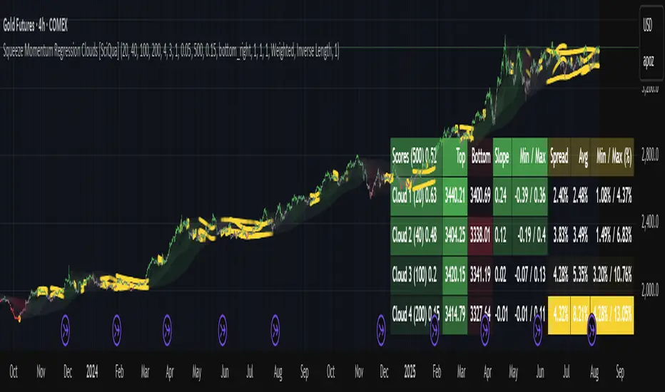
Squeeze Momentum Regression Clouds [SciQua]╭──────────────────────────────────────────────╮
☁️ Squeeze Momentum Regression Clouds
╰──────────────────────────────────────────────╯
🔍 Overview
The Squeeze Momentum Regression Clouds (SMRC) indicator is a powerful visual tool for identifying price compression , trend strength , and slope momentum using multiple layers of linear regression Clouds. Designed to extend the classic squeeze framework, this indicator captures the behavior of price through dynamic slope detection, percentile-based spread analytics, and an optional UI for trend inspection — across up to four customizable regression Clouds .
────────────────────────────────────────────────────────────
╭────────────────╮
⚙️ Core Features
╰────────────────╯
Up to 4 Regression Clouds – Each Cloud is created from a top and bottom linear regression line over a configurable lookback window.
Slope Detection Engine – Identifies whether each band is rising, falling, or flat based on slope-to-ATR thresholds.
Spread Compression Heatmap – Highlights compressed zones using yellow intensity, derived from historical spread analysis.
Composite Trend Scoring – Aggregates directional signals from each Cloud using your chosen weighting model.
Color-Coded Candles – Optional candle coloring reflects the real-time composite score.
UI Table – A toggleable info table shows slopes, compression levels, percentile ranks, and direction scores for each Cloud.
Gradient Cloud Styling – Apply gradient coloring from Cloud 1 to Cloud 4 for visual slope intensity.
Weight Aggregation Options – Use equal weighting, inverse-length weighting, or max pooling across Clouds to determine composite trend strength.
────────────────────────────────────────────────────────────
╭──────────────────────────────────────────╮
🧪 How to Use the Indicator
1. Understand Trend Bias with Cloud Colors
╰──────────────────────────────────────────╯
Each Cloud changes color based on its current slope:
Green indicates a rising trend.
Red indicates a falling trend.
Gray indicates a flat slope — often seen during chop or transitions.
Cloud 1 typically reflects short-term structure, while Cloud 4 represents long-term directional bias. Watch for multi-Cloud alignment — when all Clouds are green or red, the trend is strong. Divergence among Clouds often signals a potential shift.
────────────────────────────────────────────────────────────
╭───────────────────────────────────────────────╮
2. Use Compression Heat to Anticipate Breakouts
╰───────────────────────────────────────────────╯
The space between each Cloud’s top and bottom regression lines is measured, normalized, and analyzed over time. When this spread tightens relative to its history, the script highlights the band with a yellow compression glow .
This visual cue helps identify squeeze zones before volatility expands. If you see compression paired with a changing slope color (e.g., gray to green), this may indicate an impending breakout.
────────────────────────────────────────────────────────────
╭─────────────────────────────────╮
3. Leverage the Optional Table UI
╰─────────────────────────────────╯
The indicator includes a dynamic, floating table that displays real-time metrics per Cloud. These include:
Slope direction and value , with historical Min/Max reference.
Top and Bottom percentile ranks , showing how price sits within the Cloud range.
Current spread width , compared to its historical norms.
Composite score , which blends trend, slope, and compression for that Cloud.
You can customize the table’s position, theme, transparency, and whether to show a combined summary score in the header.
────────────────────────────────────────────────────────────
╭─────────────────────────────────────────────╮
4. Analyze Candle Color for Composite Signals
╰─────────────────────────────────────────────╯
When enabled, the indicator colors candles based on a weighted composite score. This score factors in:
The signed slope of each Cloud (up, down, or flat)
The percentile pressure from the top and bottom bands
The degree of spread compression
Expect green candles in bullish trend phases, red candles during bearish regimes, and gray candles in mixed or low-conviction zones.
Candle coloring provides a visual shorthand for market conditions , useful for intraday scanning or historical backtesting.
────────────────────────────────────────────────────────────
╭────────────────────────╮
🧰 Configuration Guidance
╰────────────────────────╯
To tailor the indicator to your strategy:
Use Cloud lengths like 21, 34, 55, and 89 for a balanced multi-timeframe view.
Adjust the slope threshold (default 0.05) to control how sensitive the trend coloring is.
Set the spread floor (e.g., 0.15) to tune when compression is detected and visualized.
Choose your weighting style : Inverse Length (favor faster bands), Equal, or Max Pooling (most aggressive).
Set composite weights to emphasize trend slope, percentile bias, or compression—depending on your market edge.
────────────────────────────────────────────────────────────
╭────────────────╮
✅ Best Practices
╰────────────────╯
Use aligned Cloud colors across all bands to confirm trend conviction.
Combine slope direction with compression glow for early breakout entry setups.
In choppy markets, watch for Clouds 1 and 2 turning flat while Clouds 3 and 4 remain directional — a sign of potential trend exhaustion or consolidation.
Keep the table enabled during backtesting to manually evaluate how each Cloud behaved during price turns and consolidations.
────────────────────────────────────────────────────────────
╭───────────────────────╮
📌 License & Usage Terms
╰───────────────────────╯
This script is provided under the Creative Commons Attribution-NonCommercial 4.0 International License .
✅ You are allowed to:
Use this script for personal or educational purposes
Study, learn, and adapt it for your own non-commercial strategies
❌ You are not allowed to:
Resell or redistribute the script without permission
Use it inside any paid product or service
Republish without giving clear attribution to the original author
For commercial licensing , private customization, or collaborations, please contact Joshua Danford directly.
BERLIN-MAX 1V.5BERLIN-MAX 1V.5 is a comprehensive trading indicator designed for TradingView that combines multiple advanced strategies and tools. It integrates EMA crossover signals, UT Bot logic with ATR-based trailing stops, customizable stop-loss and target multipliers per timeframe, Hull Moving Averages with color-coded trends, linear regression channels for support and resistance, and a multi-timeframe RSI and volume signal table. This script aims to provide clear entry and exit signals for scalping and swing trading, enhancing decision-making across different market conditions.
Adaptive Market Profile – Auto Detect & Dynamic Activity ZonesAdaptive Market Profile is an advanced indicator that automatically detects and displays the most relevant trend channel and market profile for any asset and timeframe. Unlike standard regression channel tools, this script uses a fully adaptive approach to identify the optimal period, providing you with the channel that best fits the current market dynamics. The calculation is based on maximizing the statistical significance of the trend using Pearson’s R coefficient, ensuring that the most relevant trend is always selected.
Within the selected channel, the indicator generates a dynamic market profile, breaking the price range into configurable zones and displaying the most active areas based on volume or the number of touches. This allows you to instantly identify high-activity price levels and potential support/resistance zones. The “most active lines” are plotted in real-time and always stay parallel to the channel, dynamically adapting to market structure.
Key features:
- Automatic detection of the optimal regression period: The script scans a wide range of lengths and selects the channel that statistically represents the strongest trend.
- Dynamic market profile: Visualizes the distribution of volume or price touches inside the trend channel, with customizable section count.
- Most active zones: Highlights the most traded or touched price levels as dynamic, parallel lines for precise support/resistance reading.
- Manual override: Optionally, users can select their own channel period for full control.
- Supports both linear and logarithmic charts: Simple toggle to match your chart scaling.
Use cases:
- Trend following and channel trading strategies.
- Quick identification of dynamic support/resistance and liquidity zones.
- Objective selection of the most statistically significant trend channel, without manual guesswork.
- Suitable for all assets and timeframes (crypto, stocks, forex, futures).
Originality:
This script goes beyond basic regression channels by integrating dynamic profile analysis and fully adaptive period detection, offering a comprehensive tool for modern technical analysts. The combination of trend detection, market profile, and activity zone mapping is unique and not available in TradingView built-ins.
Instructions:
Add Adaptive Market Profile to your chart. By default, the script automatically detects the optimal channel period and displays the corresponding regression channel with dynamic profile and activity zones. If you prefer manual control, disable “Auto trend channel period” and set your preferred period. Adjust profile settings as needed for your asset and timeframe.
For questions, suggestions, or further customization, contact Julien Eche (@Julien_Eche) directly on TradingView.

Dynamic S/R System - Pivot + ChannelDynamic S/R System - Pivot + Channel
A comprehensive Support & Resistance indicator combining dual methodologies for institutional-grade price level analysis
📊 CORE FEATURES
Dual Detection System
• Pivot-Based Levels - Historical turning points with intelligent touch counting
• Dynamic Channel S/R - Trend-aware linear regression boundaries
• Smart Level Management - Auto-merges similar levels, removes weak/outdated ones
Volume Integration
• Multi-timeframe volume analysis using EMA oscillator and spike detection
• Volume confirmation for all breakout signals to filter false moves
• Real-time volume status (Normal/High/Spike) in live information panel
Intelligent Touch Counting
• Automatic level validation through touch frequency analysis
• Strength classification with visual differentiation (colors/thickness)
• Level labels showing exact touch count (S3, R5, etc.)
━━━━━━━━━━━━━━━━━━━━━━━━━━━━━━━━━━━━━━━━━━━━━━━━━━━━━━━━━━━━━━━━━━━━━━━━━━━━━━━
🎨 VISUAL ELEMENTS
Line System
Solid Lines: Pivot-based S/R levels
Dashed Lines: Dynamic channel boundaries
Color Coding:
• 🔵 Blue/🔴 Red: Standard support/resistance
• 🟠 Orange: Strong levels (multiple touches)
• 🟣 Purple: Channel S/R levels
Signal Labels
• "B" - Pivot S/R breakout with volume confirmation
• "CB" - Channel boundary breakout
• "Bull/Bear Wick" - False breakout detection (wick rejections)
Information Panel
Real-time analysis displays:
• Total resistance/support levels detected
• Closest S/R levels to current price
• Volume status and position relative to levels
• Current market position assessment
━━━━━━━━━━━━━━━━━━━━━━━━━━━━━━━━━━━━━━━━━━━━━━━━━━━━━━━━━━━━━━━━━━━━━━━━━━━━━━━
✅ KEY ADVANTAGES
Multi-Method Validation
Combines historical pivot analysis with dynamic trend channels for comprehensive market view
False Breakout Protection
• Volume confirmation requirements
• Wick analysis to identify failed attempts
• Multiple validation criteria before signal generation
Adaptive Level Management
• Automatically updates as new pivots form
• Removes outdated/weak levels
• Maintains clean, relevant level display
Institutional-Grade Analysis
• Touch counting reveals institutional respect levels
• Volume integration shows smart money activity
• Strength classification identifies high-probability zones
━━━━━━━━━━━━━━━━━━━━━━━━━━━━━━━━━━━━━━━━━━━━━━━━━━━━━━━━━━━━━━━━━━━━━━━━━━━━━━━
⏰ OPTIMAL USE CASES
Best Timeframes
• Daily - Primary recommendation for swing trading
• 4-Hour - Intraday analysis and entries
• Weekly - Long-term position planning
Ideal Markets
• Crypto pairs (especially ETH/BTC, BTC/USD)
• Forex majors with good volume data
• Large-cap stocks with institutional participation
Trading Applications
• Entry/exit planning around key S/R levels
• Breakout confirmation with volume validation
• Risk management using nearest S/R for stops
• Trend analysis through channel dynamics
━━━━━━━━━━━━━━━━━━━━━━━━━━━━━━━━━━━━━━━━━━━━━━━━━━━━━━━━━━━━━━━━━━━━━━━━━━━━━━━
⚙️ CONFIGURATION GUIDELINES
Conservative Setup (Higher Confidence)
Min Pivot Strength: 3-4
Volume Threshold: 25-30%
Max Levels: 6-8
Aggressive Setup (More Signals)
Min Pivot Strength: 2
Volume Threshold: 15-20%
Max Levels: 10-12
🔔 ALERT SYSTEM
Breakout Alerts
• Resistance/Support breaks with volume confirmation
• Channel boundary violations
• Approaching strong S/R levels
Advanced Notifications
• Strong level approaches (within 0.5% of price)
• False breakout detection
• Volume spike confirmations
📈 TRADING STRATEGY GUIDE
Entry Strategy
1. Wait for price to approach identified S/R level
2. Confirm with volume analysis (spike/high volume preferred)
3. Watch for wick formations indicating rejection
4. Enter on confirmed breakout with volume or bounce with rejection
Risk Management
• Use nearest S/R level for stop placement
• Scale position size based on level strength (touch count)
• Monitor volume confirmation for exit signals
Market Context
• Combine with higher timeframe trend analysis
• Consider overall market sentiment and volatility
• Use channel direction for bias confirmation
Transform complex S/R analysis into actionable trading intelligence with institutional-level insights for professional trading decisions.

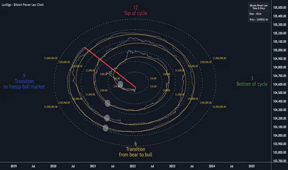
Bitcoin Power Law Clock [LuxAlgo]The Bitcoin Power Law Clock is a unique representation of Bitcoin prices proposed by famous Bitcoin analyst and modeler Giovanni Santostasi.
It displays a clock-like figure with the Bitcoin price and average lines as spirals, as well as the 12, 3, 6, and 9 hour marks as key points in the cycle.
🔶 USAGE
Giovanni Santostasi, Ph.D., is the creator and discoverer of the Bitcoin Power Law Theory. He is passionate about Bitcoin and has 12 years of experience analyzing it and creating price models.
As we can see in the above chart, the tool is super intuitive. It displays a clock-like figure with the current Bitcoin price at 10:20 on a 12-hour scale.
This tool only works on the 1D INDEX:BTCUSD chart. The ticker and timeframe must be exact to ensure proper functionality.
According to the Bitcoin Power Law Theory, the key cycle points are marked at the extremes of the clock: 12, 3, 6, and 9 hours. According to the theory, the current Bitcoin prices are in a frenzied bull market on their way to the top of the cycle.
🔹 Enable/Disable Elements
All of the elements on the clock can be disabled. If you disable them all, only an empty space will remain.
The different charts above show various combinations. Traders can customize the tool to their needs.
🔹 Auto scale
The clock has an auto-scale feature that is enabled by default. Traders can adjust the size of the clock by disabling this feature and setting the size in the settings panel.
The image above shows different configurations of this feature.
🔶 SETTINGS
🔹 Price
Price: Enable/disable price spiral, select color, and enable/disable curved mode
Average: Enable/disable average spiral, select color, and enable/disable curved mode
🔹 Style
Auto scale: Enable/disable automatic scaling or set manual fixed scaling for the spirals
Lines width: Width of each spiral line
Text Size: Select text size for date tags and price scales
Prices: Enable/disable price scales on the x-axis
Handle: Enable/disable clock handle
Halvings: Enable/disable Halvings
Hours: Enable/disable hours and key cycle points
🔹 Time & Price Dashboard
Show Time & Price: Enable/disable time & price dashboard
Location: Dashboard location
Size: Dashboard size
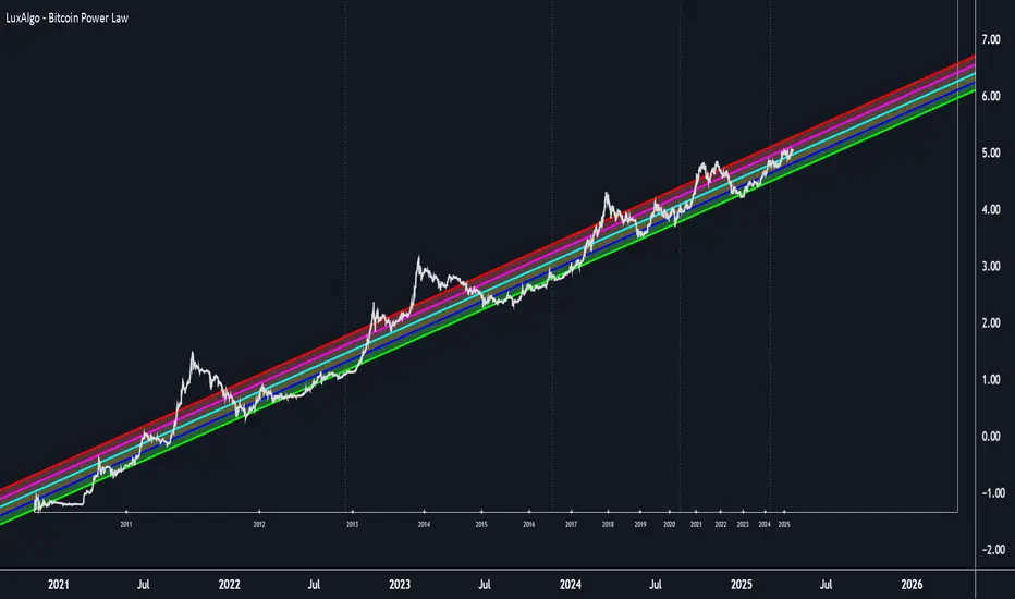
Bitcoin Power Law [LuxAlgo]The Bitcoin Power Law tool is a representation of Bitcoin prices first proposed by Giovanni Santostasi, Ph.D. It plots BTCUSD daily closes on a log10-log10 scale, and fits a linear regression channel to the data.
This channel helps traders visualise when the price is historically in a zone prone to tops or located within a discounted zone subject to future growth.
🔶 USAGE
Giovanni Santostasi, Ph.D. originated the Bitcoin Power-Law Theory; this implementation places it directly on a TradingView chart. The white line shows the daily closing price, while the cyan line is the best-fit regression.
A channel is constructed from the linear fit root mean squared error (RMSE), we can observe how price has repeatedly oscillated between each channel areas through every bull-bear cycle.
Excursions into the upper channel area can be followed by price surges and finishing on a top, whereas price touching the lower channel area coincides with a cycle low.
Users can change the channel areas multipliers, helping capture moves more precisely depending on the intended usage.
This tool only works on the daily BTCUSD chart. Ticker and timeframe must match exactly for the calculations to remain valid.
🔹 Linear Scale
Users can toggle on a linear scale for the time axis, in order to obtain a higher resolution of the price, (this will affect the linear regression channel fit, making it look poorer).
🔶 DETAILS
One of the advantages of the Power Law Theory proposed by Giovanni Santostasi is its ability to explain multiple behaviors of Bitcoin. We describe some key points below.
🔹 Power-Law Overview
A power law has the form y = A·xⁿ , and Bitcoin’s key variables follow this pattern across many orders of magnitude. Empirically, price rises roughly with t⁶, hash-rate with t¹² and the number of active addresses with t³.
When we plot these on log-log axes they appear as straight lines, revealing a scale-invariant system whose behaviour repeats proportionally as it grows.
🔹 Feedback-Loop Dynamics
Growth begins with new users, whose presence pushes the price higher via a Metcalfe-style square-law. A richer price pool funds more mining hardware; the Difficulty Adjustment immediately raises the hash-rate requirement, keeping profit margins razor-thin.
A higher hash rate secures the network, which in turn attracts the next wave of users. Because risk and Difficulty act as braking forces, user adoption advances as a power of three in time rather than an unchecked S-curve. This circular causality repeats without end, producing the familiar boom-and-bust cadence around the long-term power-law channel.
🔹 Scale Invariance & Predictions
Scale invariance means that enlarging the timeline in log-log space leaves the trajectory unchanged.
The same geometric proportions that described the first dollar of value can therefore extend to a projected million-dollar bitcoin, provided no catastrophic break occurs. Institutional ETF inflows supply fresh capital but do not bend the underlying slope; only a persistent deviation from the line would falsify the current model.
🔹 Implications
The theory assigns scarcity no direct role; iterative feedback and the Difficulty Adjustment are sufficient to govern Bitcoin’s expansion. Long-term valuation should focus on position within the power-law channel, while bubbles—sharp departures above trend that later revert—are expected punctuations of an otherwise steady climb.
Beyond about 2040, disruptive technological shifts could alter the parameters, but for the next order of magnitude the present slope remains the simplest, most robust guide.
Bitcoin behaves less like a traditional asset and more like a self-organising digital organism whose value, security, and adoption co-evolve according to immutable power-law rules.
🔶 SETTINGS
🔹 General
Start Calculation: Determine the start date used by the calculation, with any prior prices being ignored. (default - 15 Jul 2010)
Use Linear Scale for X-Axis: Convert the horizontal axis from log(time) to linear calendar time
🔹 Linear Regression
Show Regression Line: Enable/disable the central power-law trend line
Regression Line Color: Choose the colour of the regression line
Mult 1: Toggle line & fill, set multiplier (default +1), pick line colour and area fill colour
Mult 2: Toggle line & fill, set multiplier (default +0.5), pick line colour and area fill colour
Mult 3: Toggle line & fill, set multiplier (default -0.5), pick line colour and area fill colour
Mult 4: Toggle line & fill, set multiplier (default -1), pick line colour and area fill colour
🔹 Style
Price Line Color: Select the colour of the BTC price plot
Auto Color: Automatically choose the best contrast colour for the price line
Price Line Width: Set the thickness of the price line (1 – 5 px)
Show Halvings: Enable/disable dotted vertical lines at each Bitcoin halving
Halvings Color: Choose the colour of the halving lines
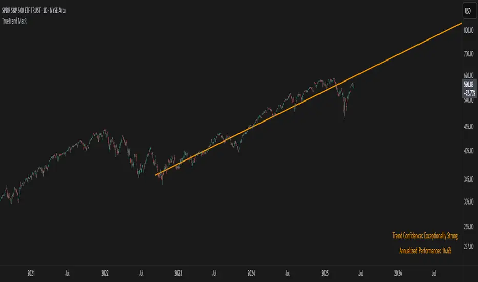
TrueTrend MaxRThe TrueTrend MaxR indicator is designed to identify the most consistent exponential price trend over extended periods. It uses statistical analysis on log-transformed prices to find the trendline that best fits historical price action, and highlights the most frequently tested or traded level within that trend channel.
For optimal results, especially on high timeframes such as weekly or monthly, it is recommended to use this indicator on charts set to logarithmic scale. This ensures proper visual alignment with the exponential nature of long-term price movements.
How it works
The indicator tests 50 different lookback periods, ranging from 300 to 1280 bars. For each period, it:
- Applies a linear regression on the natural logarithm of the price
- Computes the slope and intercept of the trendline
- Calculates the unbiased standard deviation from the regression line
- Measures the correlation strength using Pearson's R coefficient
The period with the highest Pearson R value is selected, meaning the trendline drawn corresponds to the log-scale trend with the best statistical fit.
Trendline and deviation bands
Once the optimal period is identified, the indicator plots:
- A main log-scale trendline
- Upper and lower bands, based on a user-defined multiple of the standard deviation
These bands help visualize how far price deviates from its core trend, and define the range of typical fluctuations.
Point of Control (POC)
Inside the trend channel, the space between upper and lower bands is divided into 15 logarithmic levels. The script evaluates how often price has interacted with each level, using one of two selectable methods:
- Touches: Counts the number of candles crossing each level
- Volume: Weighs each touch by the traded volume at that candle
The level with the highest cumulative interaction is considered the dynamic Point of Control (POC), and is plotted as a line.
Annualized performance and confidence display
When used on daily or weekly timeframes, the script also calculates the annualized return (CAGR) based on the detected trend, and displays:
- A performance estimate in percentage terms
- A textual label describing the confidence level based on the Pearson R value
Why this indicator is useful
- Automatically detects the most statistically consistent exponential trendline
- Designed for log-scale analysis, suited to long-term investment charts
- Highlights key price levels frequently visited or traded within the trend
- Provides objective, data-based trend and volatility insights
- Displays annualized growth rate and correlation strength for quick evaluation
Notes
- All calculations are performed only on the last bar
- No future data is used, and the script does not repaint
- Works on any instrument or timeframe, with optimal use on higher timeframes and logarithmic scaling
Linear Regression Slope The Linear Regression Slope provides a quantitative measure of trend direction. It fits a linear regression line to the past N closing prices and calculates the slope, representing the average rate of price change per bar.
To ensure comparability across assets and timeframes, the slope is normalized by the ATR over a shorter window. This produces a volatility-adjusted measure which allows for the slope to be interpreted relative to typical price fluctuations.
Mathematically, the slope is derived by minimizing the sum of squared deviations between actual prices and the fitted regression line. A positive normalized slope indicate upwards movement; a negative slope indicate downwards movement. Persistent values near zero could indicate an absence of clear trend, with price dominated by short-term fluctuations or noise.
The definition of a trend depends on the period of observation. The lookback setting should be set based on to the desired timeframe. Shorter lookbacks will respond faster to recent changes but may be more sensitive to noise, while longer lookbacks will emphasize broader structures.
While effective at quantifying existing trends, this method is not predictive. Sudden regime changes, volatility shocks, and non-linear dynamics can all cause rapid slope reversals. Therefore, it is best applied as part of a broader analytical framework.
In summary, the Linear Regression Slope quantifies price direction and serves as a measurable supplement to the visual assessment of trends on price charts.
Additional Features:
Option to display or hide the normalized slope line.
Option to enable background coloring when the slope is above or below zero.