Fakeout Kavach by Pooja v10📘 Description – Fakeout Kavach by Pooja
Fakeout Kavach by Pooja is a precision-built technical analysis tool designed for structured momentum and divergence evaluation within the RSI pane.
It helps visualize potential exhaustion zones using RSI divergence, ADX trend confirmation, and an integrated VAD (Volume + ATR + Delta) module — ensuring clarity and confirmation-based plotting.
⚙️ Core Functional Modules
1️⃣ RSI & Moving Average Module
Adaptive RSI with real-time color gradients
Optional RSI moving average (yellow) for momentum tracking
Dynamic fill zones showing overbought / oversold areas
Background fill for quick zone visualization
2️⃣ RSI Divergence Detection (Bull / Bear)
Auto-detects pivot-based bullish and bearish divergences
Non-repainting logic confirmed post-pivot formation
Smart line management with automatic cleanup
Visual divergence lines and clear on-chart markers
3️⃣ ADX Trend Confirmation
Adjustable comparison: “Higher than N bars ago” or “Higher than highest of last N”
Confirms directional strength before SB / SS signals are displayed
4️⃣ SB / SS Signal Module
“Signal Bull / Signal Sell” markers confirmed post candle closure
Integrated session-block feature to exclude specific intraday periods
Non-repainting, bar-confirmed signal plotting
5️⃣ VAD (Volume + ATR + Delta) Divergence Engine
Highlights hidden momentum shifts via volatility + volume flow logic
Bullish (B-DV) / Bearish (S-DV) divergence markers plotted at pivot bars
Customizable label or symbol-style visualization
🧩 Built-in Features
Non-repainting structure using barstate confirmation
Optimized for all timeframes and chart types
Lightweight execution with flexible styling options
Modular input control for easy customization
⚠️ Disclaimer
This indicator is for technical analysis and educational purposes only.
It does not provide financial advice, does not predict price direction, and does not guarantee profits or performance.
All trading decisions are the sole responsibility of the user. Always test thoroughly before applying to live markets.
M-oscillator

Lightning Osc • PreVersion
The Lightning Osc • PreVersion is where the MahaTrend vision began —
the first oscillator designed to visualize the pulse of the market itself.
It reveals how momentum expands, cools down, and reverses through natural rhythm,
allowing you to see balance and exhaustion with clarity and precision.
This is the original core from which every Lightning indicator later evolved —
simple, focused, and deeply intuitive.
🧭 Purpose
The indicator highlights overbought and oversold rhythm zones,
helping traders recognize when the market may have reached its energetic limits.
Rather than generating signals, it visualizes the transitions of energy
— the quiet shift that often happens before price movement changes direction.
💡 Core Logic
When the curve moves above +67.65, the market enters an overbought zone.
The most informative moment is the break below and retest of that boundary —
it often reflects fading upward strength and possible correction.
When the curve dips below −67.65, the market enters an oversold zone.
A break above and retest of this area may show that selling pressure is exhausted
and the market is ready for relief or reversal.
These levels do not dictate trades — they show rhythm
so you can understand when momentum begins to breathe again.
⏱ Recommended Timeframes
Optimized for 1-minute to 1-hour charts,
the Lightning Osc • PreVersion is most expressive on lower timeframes
where short-term volatility and energy flow are clearly visible.
🧩 How to Use
Add the indicator to a separate pane below your chart.
Choose the calculation timeframe (default: current chart TF).
Observe the curve:
Above +67.65 → Overbought zone
Below −67.65 → Oversold zone
±4.6 → Micro-pulse equilibrium
Focus on break & retest behavior near key zones —
these moments often reveal changing market rhythm.
Always confirm with your broader context and personal strategy.
🌩 Philosophy
This PreVersion marks the beginning of the Lightning language —
a balance between structure and flow,
between overextension and calm restoration.
It embodies the MahaTrend idea that the market is not chaos,
but an energy field breathing in and out through rhythm.
Disclaimer:
For educational and analytical use only.
This indicator does not provide financial advice or guaranteed results.
Always combine it with your own analysis and risk management.
— by MahaTrend

Automated Z-scoring - [JTCAPITAL]Automated Z-Scoring - is a modified way to use statistical normalization through Z-Scores for analyzing price deviations, volatility extremes, and mean reversion opportunities in financial markets.
The indicator works by calculating in the following steps:
Source Selection
The indicator begins by selecting a user-defined price source (default is the Close price). Traders can modify this to use any indicator that is deployed on the chart, for accurate and fast Z-scoring.
Mean Calculation
A Simple Moving Average (SMA) is calculated over the selected length period (default 3000). This represents the long-term equilibrium price level or the “statistical mean” of the dataset. It provides the baseline around which all price deviations are measured.
Standard Deviation Measurement
The script computes the Standard Deviation of the price series over the same period. This value quantifies how far current prices tend to stray from the mean — effectively measuring market volatility. The larger the standard deviation, the more volatile the market environment.
Z-Score Normalization
The Z-Score is calculated as:
(Current Price − Mean) ÷ Standard Deviation .
This normalization expresses how many standard deviations the current price is away from its long-term average. A Z-Score above 0 means the price is above average, while a negative score indicates it is below average.
Visual Representation
The Z-Score is plotted dynamically, with color-coding for clarity:
Bullish readings (Z > 0) are showing positive deviation from the mean.
Bearish readings (Z < 0) are showing negative deviation from the mean.
Make sure to select the correct source for what you exactly want to Z-score.
Buy and Sell Conditions:
While the indicator itself is designed as a statistical framework rather than a direct buy/sell signal generator, traders can derive actionable strategies from its behavior:
Trend Following: When the Z-Score crosses above zero after a prolonged negative period, it suggests a return to or above the mean — a possible bullish reversal or trend continuation signal.
Mean Reversion: When the Z-score is below for example -1.5 it indicates a good time for a DCA buying opportunity.
Trend Following: When the Z-Score crosses below zero after being positive, it may indicate a momentum slowdown or bearish shift.
Mean Reversion: When the Z-score is above for example 1.5 it indicates a good time for a DCA sell opportunity
Features and Parameters:
Length – Defines the period for both SMA and Standard Deviation. A longer length smooths the Z-Score and captures broader market context, while a shorter length increases responsiveness.
Source – Allows the user to choose which price data is analyzed (Close, Open, High, Low, etc.).
Fill Visualization – Highlights the magnitude of deviation between the Z-Score and the zero baseline, enhancing readability of volatility extremes.
Specifications:
Mean (Simple Moving Average)
The SMA calculates the average of the selected source over the defined length. It provides a central value to which the price tends to revert. In this indicator, the mean acts as the equilibrium point — the “zero” reference for all deviations.
Standard Deviation
Standard Deviation measures the dispersion of data points from their mean. In trading, it quantifies volatility. A high standard deviation indicates that prices are spread out (volatile), while a low value means they are clustered near the average (stable). The indicator uses this to scale deviations consistently across different market conditions.
Z-Score
The Z-Score converts raw price data into a standardized value measured in units of standard deviation.
A Z-Score of 0 = Price equals its mean.
A Z-Score of +1 = Price is one standard deviation above the mean.
A Z-Score of −1 = Price is one standard deviation below the mean.
This allows comparison of deviation magnitudes across instruments or timeframes, independent of price level.
Length Parameter
A long lookback period (e.g., 3000 bars) smooths temporary volatility and reveals long-term mean deviations — ideal for macro trend identification. Shorter lengths (e.g., 100–500) capture quicker oscillations and are useful for short-term mean reversion trades.
Statistical Interpretation
From a probabilistic perspective, if the distribution of prices is roughly normal:
About 68% of price observations lie within ±1 standard deviation (Z between −1 and +1).
About 95% lie within ±2 standard deviations.
Therefore, when the Z-Score moves beyond ±2, it statistically represents a rare event — often corresponding to price extremes or potential reversal zones.
Practical Benefit of Z-Scoring in Trading
Z-Scoring transforms raw price into a normalized volatility-adjusted metric. This allows traders to:
Compare instruments on a common statistical scale.
Identify mean-reversion setups more objectively.
Spot volatility expansions or contractions early.
Detect when price action significantly diverges from long-term equilibrium.
By automating this process, Automated Z-Scoring - provides traders with a powerful analytical lens to measure how “stretched” the market truly is — turning abstract statistics into a visually intuitive and actionable form.
Enjoy!

SigmaKernel - AdaptiveSigmaKernel - Adaptive Self-Optimizing Multi-Factor Trading System
SigmaKernel - Adaptive is a self-learning algorithmic trading strategy that combines four distinct analytical dimensions—momentum, market structure, volume flow, and reversal patterns—within a machine-learning-inspired framework that continuously adjusts its own parameters based on realized trading performance. Unlike traditional fixed-parameter strategies that maintain static weightings regardless of market conditions or results, this system implements a feedback loop that tracks which signal types, directional biases, and market conditions produce profitable outcomes, then mathematically adjusts component weightings, minimum score thresholds, position sizing multipliers, and trade spacing requirements to optimize future performance.
The strategy is designed for futures traders operating on prop firm accounts or live capital, incorporating realistic execution mechanics including configurable entry modes (stop breakout orders, limit pullback entries, or market-on-open), commission structures calibrated to retail futures contracts ($0.62 per contract default), one-tick slippage modeling, and professional risk controls including trailing drawdown guards, daily loss limits, and weekly profit targets. The system features universal futures compatibility—it automatically detects and adapts to any futures contract by reading the instrument's tick size and point value directly from the chart, eliminating the need for manual configuration across different markets.
What Makes This Approach Different
Adaptive Weight Optimization System
The core differentiation is the adaptive learning architecture. The strategy maintains four independent scoring components: momentum analysis (using RSI multi-timeframe, MACD histogram, and DMI/ADX), market structure detection (breakout identification via pivot-based support/resistance and moving average positioning), volume flow analysis (Volume Price Trend indicator with standard deviation confirmation), and reversal pattern recognition (oversold/overbought conditions combined with structural levels).
Each component generates a directional score that is multiplied by its current weight. After every closed trade, the system performs a retrospective analysis on the last N trades (configurable Learning Period, default 15 trades) to calculate win rates for each signal type independently. For example, if momentum-driven trades won 65% of the time while reversal trades won only 35%, the adaptive algorithm increases the momentum weight and decreases the reversal weight proportionally. The adjustment formula is:
New_Weight = Current_Weight + (Component_Win_Rate - Average_Win_Rate) × Adaptation_Speed
This creates a self-correcting mechanism where successful signal generators receive more influence in future composite scores, while underperforming components are de-emphasized. The system separately tracks long versus short win rates and applies directional bias corrections—if shorts consistently outperform longs, the strategy applies a 10% reduction to bullish signals to prevent fighting the prevailing market character.
Dynamic Parameter Adjustment
Beyond component weightings, three critical strategy parameters self-adjust based on performance:
Minimum Signal Score: The threshold required to trigger a trade. If overall win rate falls below 45%, the system increments this threshold by 0.10 per adjustment cycle, making the strategy more selective. If win rate exceeds 60%, the threshold decreases to allow more opportunities. This prevents the strategy from overtrading during unfavorable conditions and capitalizes on high-probability environments.
Risk Multiplier: Controls position sizing aggression. When drawdown exceeds 5%, risk per trade reduces by 10% per cycle. When drawdown falls below 2%, risk increases by 5% per cycle. This implements the professional risk management principle of "bet small when losing, bet bigger when winning" algorithmically.
Bars Between Trades: Spacing filter to prevent overtrading. Base value (default 9 bars) multiplies by drawdown factor and losing streak factor. During drawdown or consecutive losses, spacing expands up to 2x to allow market conditions to change before re-entering.
All adaptation operates during live forward-testing or real trading—there is no in-sample optimization applied to historical data. The system learns solely from its own realized trades.
Universal Futures Compatibility
The strategy implements universal futures instrument detection that automatically adapts to any futures contract without requiring manual configuration. Instead of hardcoding specific contract specifications, the system reads three critical values directly from TradingView's symbol information:
Tick Size Detection: Uses `syminfo.mintick` to obtain the minimum price increment for the current instrument. This value varies widely across markets—ES trades in 0.25 ticks, crude oil (CL) in 0.01 ticks, gold (GC) in 0.10 ticks, and treasury futures (ZB) in increments of 1/32nds. The strategy adapts all entry buffer calculations and stop placement logic to the detected tick size.
Point Value Detection: Uses `syminfo.pointvalue` to determine the dollar value per full point of price movement. For ES, one point equals $50; for crude oil, one point equals $1,000; for gold, one point equals $100. This automatic detection ensures accurate P&L calculations and risk-per-contract measurements across all instruments.
Tick Value Calculation: Combines tick size and point value to compute dollar value per tick: Tick_Value = Tick_Size × Point_Value. This derived value drives all position sizing calculations, ensuring the risk management system correctly accounts for each instrument's economic characteristics.
This universal approach means the strategy functions identically on emini indices (ES, MES, NQ, MNQ), micro indices, energy contracts (CL, NG, RB), metals (GC, SI, HG), agricultural futures (ZC, ZS, ZW), treasury futures (ZB, ZN, ZF), currency futures (6E, 6J, 6B), and any other futures contract available on TradingView. No parameter adjustments or instrument-specific branches exist in the code—the adaptation happens automatically through symbol information queries.
Stop-Out Rate Monitoring System
The strategy includes an intelligent stop-out rate tracking system that monitors the percentage of your last 20 trades (or available trades if fewer than 20) that were stopped out. This metric appears in the dashboard's Performance section with color-coded guidance:
Green (<30% stop-out rate): Very few trades are being stopped out. This suggests either your stops are too loose (giving back profits on reversals) or you're in an exceptional trending market. Consider tightening your Stop Loss ATR multiplier to lock in profits more efficiently.
Orange (30-65% stop-out rate): Healthy range. Your stop placement is appropriately sized for current market conditions and the strategy's risk-reward profile. No adjustment needed.
Red (>65% stop-out rate): Too many trades are being stopped out prematurely. Your stops are likely too tight for the current volatility regime. Consider widening your Stop Loss ATR multiplier to give trades more room to develop.
Critical Design Philosophy: Unlike some systems that automatically adjust stops based on performance statistics, this strategy intentionally keeps stop-loss control in the user's hands. Automatic stop adjustment creates dangerous feedback loops—widening stops increases risk per contract, which forces position size reduction, which distorts performance metrics, leading to incorrect adaptations. Instead, the dashboard provides visibility into stop performance, empowering you to make informed manual adjustments when warranted. This preserves the integrity of the adaptive system while giving you the critical data needed for stop optimization.
Execution Kernel Architecture
The entry system offers three distinct execution modes to match trader preference and market character:
StopBreakout Mode: Places buy-stop orders above the prior bar's high (for longs) or sell-stop orders below the prior bar's low (for shorts), plus a 2-tick buffer. This ensures entries only occur when price confirms directional momentum by breaking recent structure. Ideal for trending and momentum-driven markets.
LimitPullback Mode: Places limit orders at a pullback price calculated as: Entry_Price = Close - (ATR × Pullback_Multiplier) for longs, or Close + (ATR × Pullback_Multiplier) for shorts. Default multiplier is 0.5 ATR. This waits for mean-reversion before entering in the signal direction, capturing better prices in volatile or oscillating markets.
MarketNextOpen Mode: Executes at market on the bar immediately following signal generation. This provides fastest execution but sacrifices the filtering effect of requiring price confirmation.
All pending entry orders include a configurable Time-To-Live (TTL, default 6 bars). If an order is not filled within the TTL period, it cancels automatically to prevent stale signals from executing in changed market conditions.
Professional Exit Management
The exit system implements a three-stage progression: initial stop loss, breakeven adjustment, and dynamic trailing stop.
Initial Stop Loss: Calculated as entry price ± (ATR × User_Stop_Multiplier × Volatility_Adjustment). Users have direct control via the Stop Loss ATR multiplier (default 1.25). The system then applies volatility regime adjustments: ×1.2 in high-volatility environments (stops automatically widen), ×0.8 in low volatility (stops tighten), ×1.0 in normal conditions. This ensures stops adapt to market character while maintaining user control over baseline risk tolerance.
Breakeven Trigger: When profit reaches a configurable multiple of initial risk (default 1.0R), the stop loss automatically moves to breakeven (entry price). This locks in zero-loss status once the trade demonstrates favorable movement.
Trailing Stop Activation: When profit reaches the Trail_Trigger_R multiple (default 1.2R), the system cancels the fixed stop and activates a dynamic trailing stop. The trail uses Step and Offset parameters defined in R-multiples. For example, with Trail_Offset_R = 1.0 and Trail_Step_R = 1.5, the stop trails 1.0R behind price and moves in 1.5R increments. This captures extended moves while protecting accumulated profit.
Additional failsafes include maximum time-in-trade (exits after N bars if specified) and end-of-session flatten (automatically closes all positions X minutes before session end to avoid overnight exposure).
Core Calculation Methodology
Signal Component Scoring
Momentum Component:
- Calculates 14-period DMI (Directional Movement Index) with ADX strength filter (trending when ADX > 25)
- Computes three RSI timeframes: fast (7-period), medium (14-period), slow (21-period)
- Analyzes MACD (12/26/9) histogram for directional acceleration
- Bullish momentum: uptrend (DI+ > DI- with ADX > 25) + MACD histogram rising above zero + RSI fast between 50-80 = +1.6 score
- Bearish momentum: downtrend (DI- > DI+ with ADX > 25) + MACD histogram falling below zero + RSI fast between 20-50 = -1.6 score
- Score multiplies by volatility adjustment factor: ×0.8 in high volatility (momentum less reliable), ×1.2 in low volatility (momentum more persistent)
Structure Component:
- Identifies swing highs and lows using 10-bar pivot lookback on both sides
- Maintains most recent swing high as dynamic resistance, most recent swing low as dynamic support
- Detects breakouts: bullish when close crosses above resistance with prior bar below; bearish when close crosses below support with prior bar above
- Breakout score: ±1.0 for confirmed break
- Moving average alignment: +0.5 when price > SMA20 > SMA50 (bullish structure); -0.5 when price < SMA20 < SMA50 (bearish structure)
- Total structure range: -1.5 to +1.5
Volume Component:
- Calculates Volume Price Trend: VPT = Σ [(Close - Close ) / Close × Volume]
- Compares VPT to its 10-period EMA as signal line (similar to MACD logic)
- Computes 20-period volume moving average and standard deviation
- High volume event: current volume > (volume_average + 1× std_dev)
- Bullish volume: VPT > VPT_signal AND high_volume = +1.0
- Bearish volume: VPT < VPT_signal AND high_volume = -1.0
- No score if volume is not elevated (filters out low-conviction moves)
Reversal Component:
- Identifies extreme RSI conditions: RSI slow < 30 (oversold) or > 70 (overbought)
- Requires structural confluence: price at or below support level for bullish reversal; at or above resistance for bearish reversal
- Requires momentum shift: RSI fast must be rising (for bull) or falling (for bear) to confirm reversal in progress
- Bullish reversal: RSI < 30 AND price ≤ support AND RSI rising = +1.0
- Bearish reversal: RSI > 70 AND price ≥ resistance AND RSI falling = -1.0
Composite Score Calculation
Final_Score = (Momentum × Weight_M) + (Structure × Weight_S) + (Volume × Weight_V) + (Reversal × Weight_R)
Initial weights: Momentum = 1.0, Structure = 1.2, Volume = 0.8, Reversal = 0.6
These weights adapt after each trade based on component-specific performance as described above.
The system also applies directional bias adjustment: if recent long trades have significantly lower win rate than shorts, bullish scores multiply by 0.9 to reduce aggressive long entries. Vice versa for underperforming shorts.
Position Sizing Algorithm
The position sizing calculation incorporates multiple confidence factors and automatically scales to any futures contract:
1. Base risk amount = Account_Size × Base_Risk_Percent × Adaptive_Risk_Multiplier
2. Stop distance in price units = ATR × User_Stop_Multiplier × Volatility_Regime_Multiplier × Entry_Buffer
3. Risk per contract = Stop_Distance × Dollar_Per_Point (automatically detected from instrument)
4. Raw position size = Risk_Amount / Risk_Per_Contract
Then applies confidence scaling:
- Signal confidence = min(|Weighted_Score| / Min_Score_Threshold, 2.0) — higher scores receive larger size, capped at 2×
- Direction confidence = Long_Win_Rate (for bulls) or Short_Win_Rate (for bears)
- Type confidence = Win_Rate of dominant signal type (momentum/structure/volume/reversal)
- Total confidence = (Signal_Confidence + Direction_Confidence + Type_Confidence) / 3
Adjusted size = Raw_Size × Total_Confidence × Losing_Streak_Reduction
Losing streak reduction = 0.5 if losing_streak ≥ 5, otherwise 1.0
Universal Maximum Position Calculation: Instead of hardcoded limits per instrument, the system calculates maximum position size as: Max_Contracts = Account_Size / 25000, clamped between 1 and 10 contracts. This means a $50,000 account allows up to 2 contracts, a $100,000 account allows up to 4 contracts, regardless of which futures contract is being traded. This universal approach maintains consistent risk exposure across different instruments while preventing overleveraging.
Final size is rounded to integer and bounded by the calculated maximum.
Session and Risk Management System
Timezone-Aware Session Control
The strategy implements timezone-correct session filtering. Users specify session start hour, end hour, and timezone from 12 supported zones (New York, Chicago, Los Angeles, London, Frankfurt, Moscow, Tokyo, Hong Kong, Shanghai, Singapore, Sydney, UTC). The system converts bar timestamps to the selected timezone before applying session logic.
For split sessions (e.g., Asian session 18:00-02:00), the logic correctly handles time wraparound. Weekend trading can be optionally disabled (default: disabled) to avoid low-liquidity weekend price action.
Multi-Layer Risk Controls
Daily Loss Limit: Strategy ceases all new entries when daily P&L reaches negative threshold (default $2,000). This prevents catastrophic drawdown days. Resets at timezone-corrected day boundary.
Weekly Profit Target: Strategy ceases trading when weekly profit reaches target (default $10,000). This implements the professional principle of "take the win and stop pushing luck." Resets on timezone-corrected Monday.
Maximum Daily Trades: Hard cap on entries per day (default 20) to prevent overtrading during volatile conditions when many signals may generate.
Trailing Drawdown Guard: Optional prop-firm-style trailing stop on account equity. When enabled, if equity drops below (Peak_Equity - Trailing_DD_Amount), all trading halts. This simulates the common prop firm rule where exceeding trailing drawdown results in account termination.
All limits display status in the real-time dashboard, showing "MAX LOSS HIT", "WEEKLY TARGET MET", or "ACTIVE" depending on current state.
How To Use This Strategy
Initial Setup
1. Apply the strategy to your desired futures chart (tested on 5-minute through daily timeframes)
2. The strategy will automatically detect your instrument's specifications—no manual configuration needed for different contracts
3. Configure your account size and risk parameters in the Core Settings section
4. Set your trading session hours and timezone to match your availability
5. Adjust the Stop Loss ATR multiplier based on your risk tolerance (0.8-1.2 for tighter stops, 1.5-2.5 for wider stops)
6. Select your preferred entry execution mode (recommend StopBreakout for beginners)
7. Enable adaptation (recommended) or disable for fixed-parameter operation
8. Review the strategy's Properties in the Strategy Tester settings and verify commission/slippage match your broker's actual costs
The universal futures detection means you can switch between ES, NQ, CL, GC, ZB, or any other futures contract without changing any strategy parameters—the system will automatically adapt its calculations to each instrument's unique specifications.
Dashboard Interpretation
The strategy displays a comprehensive real-time dashboard in the top-right corner showing:
Market State Section:
- Trend: Shows UPTREND/DOWNTREND/CONSOLIDATING/NEUTRAL based on ADX and DMI analysis
- ADX Value: Current trend strength (>25 = strong trend, <20 = consolidating)
- Momentum: BULL/BEAR/NEUTRAL classification with current momentum score
- Volatility: HIGH/LOW/NORMAL regime with ATR percentage of price
Volume Profile Section (Large dashboard only):
- VPT Flow: Directional bias from volume analysis
- Volume Status: HIGH/LOW/NORMAL with relative volume multiplier
Performance Section:
- Daily P&L: Current day's profit/loss with color coding
- Daily Trades: Number of completed trades today
- Weekly P&L: Current week's profit/loss
- Target %: Progress toward weekly profit target
- Stop-Out Rate: Percentage of last 20 trades (or available trades if <20) that were stopped out. Includes all stop types: initial stops, breakeven stops, trailing stops, timeout exits, and EOD flattens. Color coded with actionable guidance:
- Green (<30%): Shows "TIGHTEN" guidance. Very few stop-outs suggests stops may be too loose or exceptional market conditions. Consider reducing Stop Loss ATR multiplier.
- Orange (30-65%): Shows "OK" guidance. Healthy stop-out rate indicating appropriate stop placement for current conditions.
- Red (>65%): Shows "WIDEN" guidance. Too many premature stop-outs. Consider increasing Stop Loss ATR multiplier to give trades more room.
- Status: Overall trading status (ACTIVE/MAX LOSS HIT/WEEKLY TARGET MET/FILTERS ACTIVE)
Adaptive Engine Section:
- Min Score: Current minimum threshold for trade entry (higher = more selective)
- Risk Mult: Current position sizing multiplier (adjusts with performance)
- Bars BTW: Current minimum bars required between trades
- Drawdown: Current drawdown percentage from equity peak
- Weights: M/S/V/R showing current component weightings
Win Rates Section:
- Type: Win rates for Momentum, Structure, Volume, Reversal signal types
- Direction: Win rates for Long vs Short trades
Color coding shows green for >50% win rate, red for <50%
Session Info Section:
- Session Hours: Active trading window with timezone
- Weekend Trading: ENABLED/DISABLED status
- Session Status: ACTIVE/INACTIVE based on current time
Signal Generation and Entry
The strategy generates entries when the weighted composite score exceeds the adaptive minimum threshold (initial value configurable, typically 1.5 to 2.5). Entries display as layered triangle markers on the chart:
- Long Signal: Three green upward triangles below the entry bar
- Short Signal: Three red downward triangles above the entry bar
Triangle tooltip shows the signal score and dominant signal type (MOMENTUM/STRUCTURE/VOLUME/REVERSAL).
Position Management and Stop Optimization
Once entered, the strategy automatically manages the position through its three-stage exit system. Monitor the Stop-Out Rate metric in the dashboard to optimize your stop placement:
If Stop-Out Rate is Green (<30%): You're rarely being stopped out. This could mean:
- Your stops are too loose, allowing trades to give back too much profit on reversals
- You're in an exceptional trending market where tight stops would work better
- Action: Consider reducing your Stop Loss ATR multiplier by 0.1-0.2 to tighten stops and lock in profits more efficiently
If Stop-Out Rate is Orange (30-65%): Optimal range. Your stops are appropriately sized for the strategy's risk-reward profile and current market volatility. No adjustment needed.
If Stop-Out Rate is Red (>65%): You're being stopped out too frequently. This means:
- Your stops are too tight for current market volatility
- Trades need more room to develop before reaching profit targets
- Action: Increase your Stop Loss ATR multiplier by 0.1-0.3 to give trades more breathing room
Remember: The stop-out rate calculation includes all exit types (initial stops, breakeven stops, trailing stops, timeouts, EOD flattens). A trade that reaches breakeven and gets stopped out at entry price counts as a stop-out, even though it didn't lose money. This is intentional—it indicates the stop placement didn't allow the trade to develop into profit.
Optimization Workflow
For traders wanting to customize the strategy for their specific instrument and timeframe:
Week 1-2: Run with defaults, adaptation enabled
Allow the system to execute at least 30-50 trades (the Learning Period plus additional buffer). Monitor which session periods, signal types, and market conditions produce the best results. Observe your stop-out rate—if it's consistently red or green, plan to adjust Stop Loss ATR multiplier after the learning period. Do not adjust parameters yet—let the adaptive system establish baseline performance data.
Week 3-4: Analyze adaptation behavior and optimize stops
Review the dashboard's adaptive weights and win rates. If certain signal types consistently show <40% win rate, consider slightly reducing their base weight. If a particular entry mode produces better fill quality and win rate, switch to that mode. If you notice the minimum score threshold has climbed very high (>3.0), market conditions may not suit the strategy's logic—consider switching instruments or timeframes.
Based on your Stop-Out Rate observations:
- Consistently <30%: Reduce Stop Loss ATR multiplier by 0.2-0.3
- Consistently >65%: Increase Stop Loss ATR multiplier by 0.2-0.4
- Oscillating between zones: Leave stops at default and let volatility regime adjustments handle it
Ongoing: Fine-tune risk and execution
Adjust the following based on your risk tolerance and account type:
- Base Risk Per Trade: 0.5% for conservative, 0.75% for moderate, 1.0% for aggressive
- Stop Loss ATR Multiplier: 0.8-1.2 for tight stops (scalping), 1.5-2.5 for wide stops (swing trading)
- Bars Between Trades: Lower (5-7) for more opportunities, higher (12-20) for more selective
- Entry Mode: Experiment between modes to find best fit for current market character
- Session Hours: Narrow to specific high-performance session windows if certain hours consistently underperform
Never adjust: Do not manually modify the adaptive weights, minimum score, or risk multiplier after the system has begun learning. These parameters are self-optimizing and manual interference defeats the adaptive mechanism.
Parameter Descriptions and Optimization Guidelines
Adaptive Intelligence Group
Enable Self-Optimization (default: true): Master switch for the adaptive learning system. When enabled, component weights, minimum score, risk multiplier, and trade spacing adjust based on realized performance. Disable to run the strategy with fixed parameters (useful for comparing adaptive vs non-adaptive performance).
Learning Period (default: 15 trades): Number of most recent trades to analyze for performance calculations. Shorter values (10-12) adapt more quickly to recent conditions but may overreact to variance. Longer values (20-30) produce more stable adaptations but respond slower to regime changes. For volatile markets, use shorter periods. For stable trends, use longer periods.
Adaptation Speed (default: 0.25): Controls the magnitude of parameter adjustments per learning cycle. Lower values (0.05-0.15) make gradual, conservative changes. Higher values (0.35-0.50) make aggressive adjustments. Faster adaptation helps in rapidly changing markets but increases parameter instability. Start with default and increase only if you observe the system failing to adapt quickly enough to obvious performance patterns.
Performance Memory (default: 100 trades): Maximum number of historical trades stored for analysis. This array size does not affect learning (which uses only Learning Period trades) but provides data for future analytics features including stop-out rate tracking. Higher values consume more memory but provide richer historical dataset. Typical users should not need to modify this.
Core Settings Group
Account Size (default: $50,000): Starting capital for position sizing calculations. This should match your actual account size for accurate risk per trade. The strategy uses this value to calculate dollar risk amounts and determine maximum position size (1 contract per $25,000).
Weekly Profit Target (default: $10,000): When weekly P&L reaches this value, the strategy stops taking new trades for the remainder of the week. This implements a "quit while ahead" rule common in professional trading. Set to a realistic weekly goal—20% of account size per week ($10K on $50K) is very aggressive; 5-10% is more sustainable.
Max Daily Loss (default: $2,000): When daily P&L reaches this negative threshold, strategy stops all new entries for the day. This is your maximum acceptable daily loss. Professional traders typically set this at 2-4% of account size. A $2,000 loss on a $50,000 account = 4%.
Base Risk Per Trade % (default: 0.5%): Initial percentage of account to risk on each trade before adaptive multiplier and confidence scaling. 0.5% is conservative, 0.75% is moderate, 1.0-1.5% is aggressive. Remember that actual risk per trade = Base Risk × Adaptive Risk Multiplier × Confidence Factors, so the realized risk will vary.
Trade Filters Group
Base Minimum Signal Score (default: 1.5): Initial threshold that composite weighted score must exceed to generate a signal. Lower values (1.0-1.5) produce more trades with lower average quality. Higher values (2.0-3.0) produce fewer, higher-quality setups. This value adapts automatically when adaptive mode is enabled, but the base sets the starting point. For trending markets, lower values work well. For choppy markets, use higher values.
Base Bars Between Trades (default: 9): Minimum bars that must elapse after an entry before another signal can trigger. This prevents overtrading and allows previous trades time to develop. Lower values (3-6) suit scalping on lower timeframes. Higher values (15-30) suit swing trading on higher timeframes. This value also adapts based on drawdown and losing streaks.
Max Daily Trades (default: 20): Hard limit on total trades per day regardless of signal quality. This prevents runaway trading during extremely volatile days when many signals may generate. For 5-minute charts, 20 trades/day is reasonable. For 1-hour charts, 5-10 trades/day is more typical.
Session Group
Session Start Hour (default: 5): Hour (0-23 format) when trading is allowed to begin, in the timezone specified. For US futures trading in Chicago time, session typically starts at 5:00 or 6:00 PM (17:00 or 18:00) Sunday evening.
Session End Hour (default: 17): Hour when trading stops and no new entries are allowed. For US equity index futures, regular session ends at 4:00 PM (16:00) Central Time.
Allow Weekend Trading (default: false): Whether strategy can trade on Saturday/Sunday. Most futures have low volume on weekends; keeping this disabled is recommended unless you specifically trade Sunday evening open.
Session Timezone (default: America/Chicago): Timezone for session hour interpretation. Select your local timezone or the timezone of your instrument's primary exchange. This ensures session logic aligns with your intended trading hours.
Prop Guards Group
Trailing Drawdown Guard (default: false): Enables prop-firm-style trailing maximum drawdown. When enabled, if equity drops below (Peak Equity - Trailing DD Amount), all trading halts for the remainder of the backtest/live session. This simulates rules used by funded trader programs where exceeding trailing drawdown terminates the account.
Trailing DD Amount (default: $2,500): Dollar amount of drawdown allowed from equity peak. If your equity reaches $55,000, the trailing stop sets at $52,500. If equity then drops to $52,499, the guard triggers and trading ceases.
Execution Kernel Group
Entry Mode (default: StopBreakout):
- StopBreakout: Places stop orders above/below signal bar requiring price confirmation
- LimitPullback: Places limit orders at pullback prices seeking better fills
- MarketNextOpen: Executes immediately at market on next bar
Limit Offset (default: 0.5x ATR): For LimitPullback mode, how far below/above current price to place the limit order. Smaller values (0.3-0.5) seek minor pullbacks. Larger values (0.8-1.2) wait for deeper retracements but may miss trades.
Entry TTL (default: 6 bars, 0=off): Bars an entry order remains pending before cancelling. Shorter values (3-4) keep signals fresh. Longer values (8-12) allow more time for fills but risk executing stale signals. Set to 0 to disable TTL (orders remain active indefinitely until filled or opposite signal).
Exits Group
Stop Loss (default: 1.25x ATR): Base stop distance as a multiple of the 14-period ATR. This is your primary risk control parameter and directly impacts your stop-out rate. Lower values (0.8-1.0) create tighter stops that reduce risk per trade but may get stopped out prematurely in volatile conditions—expect stop-out rates above 65% (red zone). Higher values (1.5-2.5) give trades more room to breathe but increase risk per contract—expect stop-out rates below 30% (green zone). The system applies additional volatility regime adjustments on top of this base: ×1.2 in high volatility environments (stops widen automatically), ×0.8 in low volatility (stops tighten), ×1.0 in normal conditions. For scalping on lower timeframes, use 0.8-1.2. For swing trading on higher timeframes, use 1.5-2.5. Monitor the Stop-Out Rate metric in the dashboard and adjust this parameter to keep it in the healthy 30-65% orange zone.
Move to Breakeven at (default: 1.0R): When profit reaches this multiple of initial risk, stop moves to breakeven. 1.0R means after price moves in your favor by the distance you risked, you're protected at entry price. Lower values (0.5-0.8R) lock in breakeven faster. Higher values (1.5-2.0R) allow more room before protection.
Start Trailing at (default: 1.2R): When profit reaches this multiple, the fixed stop transitions to a dynamic trailing stop. This should be greater than the BE trigger. Values typically range 1.0-2.0R depending on how much profit you want secured before trailing activates.
Trail Offset (default: 1.0R): How far behind price the trailing stop follows. Tighter offsets (0.5-0.8R) protect profit more aggressively but may exit prematurely. Wider offsets (1.5-2.5R) allow more room for profit to run but risk giving back more on reversals.
Trail Step (default: 1.5R): How far price must move in profitable direction before the stop advances. Smaller steps (0.5-1.0R) move the stop more frequently, tightening protection continuously. Larger steps (2.0-3.0R) move the stop less often, giving trades more breathing room.
Max Bars In Trade (default: 0=off): Maximum bars allowed in a position before forced exit. This prevents trades from "going stale" during periods of no meaningful price action. For 5-minute charts, 50-100 bars (4-8 hours) is reasonable. For daily charts, 5-10 bars (1-2 weeks) is typical. Set to 0 to disable.
Flatten near Session End (default: true): Whether to automatically close all positions as session end approaches. Recommended to avoid carrying positions into off-hours with low liquidity.
Minutes before end (default: 5): How many minutes before session end to flatten. 5-15 minutes provides buffer for order execution before the session boundary.
Visual Effects Configuration Group
Dashboard Size (default: Normal): Controls information density in the dashboard. Small shows only critical metrics (excludes stop-out rate). Normal shows comprehensive data including stop-out rate. Large shows all available metrics including weights, session info, and volume analysis. Larger sizes consume more screen space but provide complete visibility.
Show Quantum Field (default: true): Displays animated grid pattern on the chart indicating market state. Disable if you prefer cleaner charts or experience performance issues on lower-end hardware.
Show Wick Pressure Lines (default: true): Draws dynamic lines from bars with extreme wicks, indicating potential support/resistance or liquidity absorption zones. Disable for simpler visualization.
Show Morphism Energy Beams (default: true): Displays directional beams showing momentum energy flow. Beams intensify during strong trends. Disable if you find this visually distracting.
Show Order Flow Clouds (default: true): Draws translucent boxes representing volume flow bullish/bearish bias. Disable for cleaner price action visibility.
Show Fractal Grid (default: true): Displays multi-timeframe support/resistance levels based on fractal price structure at 10/20/30/40/50 bar periods. Disable if you only want to see primary pivot levels.
Glow Intensity (default: 4): Controls the brightness and thickness of visual effects. Lower values (1-2) for subtle visualization. Higher values (7-10) for maximum visibility but potentially cluttered charts.
Color Theme (default: Cyber): Visual color scheme. Cyber uses cyan/magenta futuristic colors. Quantum uses aqua/purple. Matrix uses green/red terminal style. Aurora uses pastel pink/purple gradient. Choose based on personal preference and monitor calibration.
Show Watermark (default: true): Displays animated watermark at bottom of chart with creator credit and current P&L. Disable if you want completely clean charts or need screen space.
Performance Characteristics and Best Use Cases
Optimal Conditions
This strategy performs best in markets exhibiting:
Trending phases with periodic pullbacks: The combination of momentum and structure components excels when price establishes directional bias but provides retracement opportunities for entries. Markets with 60-70% trending bars and 30-40% consolidation produce the highest win rates.
Medium to high volatility: The ATR-based stop sizing and dynamic risk adjustment require sufficient price movement to generate meaningful profit relative to risk. Instruments with 2-4% daily ATR relative to price work well. Extremely low volatility (<1% daily ATR) generates too many scratch trades.
Clear volume patterns: The VPT volume component adds significant edge when volume expansions align with directional moves. Instruments and timeframes where volume data reflects actual transaction flow (versus tick volume proxies) perform better.
Regular session structure: Futures markets with defined opening and closing hours, consistent liquidity throughout the session, and clear overnight/day session separation allow the session controls and time-based failsafes to function optimally.
Sufficient liquidity for stop execution: The stop breakout entry mode requires that stop orders can fill without significant slippage. Highly liquid contracts work better than illiquid instruments where stop orders may face adverse fills.
Suboptimal Conditions
The strategy may struggle with:
Extreme chop with no directional persistence: When ADX remains below 15 for extended periods and price oscillates rapidly without establishing trends, the momentum component generates conflicting signals. Win rate typically drops below 40% in these conditions, triggering the adaptive system to increase minimum score thresholds until conditions improve. Stop-out rates may also spike into the red zone.
Gap-heavy instruments: Markets with frequent overnight gaps disrupt the continuous price assumptions underlying ATR stops and EMA-based structure analysis. Gaps can also cause stop orders to fill at prices far from intended levels, distorting stop-out rate metrics.
Very low timeframes with excessive noise: On 1-minute or tick charts, the signal components react to micro-structure noise rather than meaningful price swings. The strategy works best on 5-minute through daily timeframes where price movements reflect actual order flow shifts.
Extended low-volatility compression: During historically low volatility periods, profit targets become difficult to reach before mean-reversion occurs. The trail offset, even when set to minimum, may be too wide for the compressed price environment. Stop-out rates may drop to green zone indicating stops should be tightened.
Parabolic moves or climactic exhaustion: Vertical price advances or selloffs where price moves multiple ATRs in single bars can trigger momentum signals at exhaustion points. The structure and reversal components attempt to filter these, but extreme moves may override normal logic.
The adaptive learning system naturally reduces signal frequency and position sizing during unfavorable conditions. If you observe multiple consecutive days with zero trades and "FILTERS ACTIVE" status, this indicates the strategy has self-adjusted to avoid poor conditions rather than forcing trades.
Instrument Recommendations
Emini Index Futures (ES, MES, NQ, MNQ, YM, RTY): Excellent fit. High liquidity, clear volatility patterns, strong volume signals, defined session structure. These instruments have been extensively tested and the universal detection handles all contract specifications automatically.
Micro Index Futures (MES, MNQ, M2K, MYM): Excellent fit for smaller accounts. Same market characteristics as the standard eminis but with reduced contract sizes allowing proper risk management on accounts below $50,000.
Energy Futures (CL, NG, RB, HO): Good to mixed fit. Crude oil (CL) works well due to strong trends and reasonable volatility. Natural gas (NG) can be extremely volatile—consider reducing Base Risk to 0.3-0.4% and increasing Stop Loss ATR multiplier to 1.8-2.2 for NG. The strategy automatically detects the $10/tick value for CL and adjusts position sizing accordingly.
Metal Futures (GC, SI, HG, PL): Good fit. Gold (GC) and silver (SI) exhibit clear trending behavior and work well with the momentum/structure components. The strategy automatically handles the different point values ($100/point for gold, $5,000/point for silver).
Agricultural Futures (ZC, ZS, ZW, ZL): Good fit. Grain futures often trend strongly during seasonal periods. The strategy handles the unique tick sizes (1/4 cent increments) and point values ($50/point for corn/wheat, $60/point for soybeans) automatically.
Treasury Futures (ZB, ZN, ZF, ZT): Good fit for trending rates environments. The strategy automatically handles the fractional tick sizing (32nds for ZB/ZN, halves of 32nds for ZF/ZT) through the universal detection system.
Currency Futures (6E, 6J, 6B, 6A, 6C): Good fit. Major currency pairs exhibit smooth trending behavior. The strategy automatically detects point values which vary significantly ($12.50/tick for 6E, $12.50/tick for 6J, $6.25/tick for 6B).
Cryptocurrency Futures (BTC, ETH, MBT, MET): Mixed fit. These markets have extreme volatility requiring parameter adjustment. Increase Base Risk to 0.8-1.2% and Stop Loss ATR multiplier to 2.0-3.0 to account for wider stop distances. Enable 24-hour trading and weekend trading as these markets have no traditional sessions.
The universal futures compatibility means you can apply this strategy to any of these markets without code modification—simply open the chart of your desired contract and the strategy will automatically configure itself to that instrument's specifications.
Important Disclaimers and Realistic Expectations
This is a sophisticated trading strategy that combines multiple analytical methods within an adaptive framework designed for active traders who will monitor performance and market conditions. It is not a "set and forget" fully automated system, nor should it be treated as a guaranteed profit generator.
Backtesting Realism and Limitations
The strategy includes realistic trading costs and execution assumptions:
- Commission: $0.62 per contract per side (accurate for many retail futures brokers)
- Slippage: 1 tick per entry and exit (conservative estimate for liquid futures)
- Position sizing: Realistic risk percentages and maximum contract limits based on account size
- No repainting: All calculations use confirmed bar data only—signals do not change retroactively
However, backtesting cannot fully capture live trading reality:
- Order fill delays: In live trading, stop and limit orders may not fill instantly at the exact tick shown in backtest
- Volatile periods: During high volatility or low liquidity (news events, rollover days, pre-holidays), slippage may exceed the 1-tick assumption significantly
- Gap risk: The backtest assumes stops fill at stop price, but gaps can cause fills far beyond intended exit levels
- Psychological factors: Seeing actual capital at risk creates emotional pressures not present in backtesting, potentially leading to premature manual intervention
The strategy's backtest results should be viewed as best-case scenarios. Real trading will typically produce 10-30% lower returns than backtest due to the above factors.
Risk Warnings
All trading involves substantial risk of loss. The adaptive learning system can improve parameter selection over time, but it cannot predict future price movements or guarantee profitable performance. Past wins do not ensure future wins.
Losing streaks are inevitable. Even with a 60% win rate, you will encounter sequences of 5, 6, or more consecutive losses due to normal probability distributions. The strategy includes losing streak detection and automatic risk reduction, but you must have sufficient capital to survive these drawdowns.
Market regime changes can invalidate learned patterns. If the strategy learns from 50 trades during a trending regime, then the market shifts to a ranging regime, the adapted parameters may initially be misaligned with the new environment. The system will re-adapt, but this transition period may produce suboptimal results.
Prop firm traders: understand your specific rules. Every prop firm has different rules regarding maximum drawdown, daily loss limits, consistency requirements, and prohibited trading behaviors. While this strategy includes common prop guardrails, you must verify it complies with your specific firm's rules and adjust parameters accordingly.
Never risk capital you cannot afford to lose. This strategy can produce substantial drawdowns, especially during learning periods or market regime shifts. Only trade with speculative capital that, if lost, would not impact your financial stability.
Recommended Usage
Paper trade first: Run the strategy on a simulated account for at least 50 trades or 1 month before committing real capital. Observe how the adaptive system behaves, identify any patterns in losing trades, monitor your stop-out rate trends, and verify your understanding of the entry/exit mechanics.
Start with minimum position sizing: When transitioning to live trading, reduce the Base Risk parameter to 0.3-0.4% initially (vs 0.5-1.0% in testing) to reduce early impact while the system learns your live broker's execution characteristics.
Monitor daily, but do not micromanage: Check the dashboard daily to ensure the strategy is operating normally and risk controls have not triggered unexpectedly. Pay special attention to the Stop-Out Rate metric—if it remains in the red or green zones for multiple days, adjust your Stop Loss ATR multiplier accordingly. However, resist the urge to manually adjust adaptive weights or disable trades based on short-term performance. Allow the adaptive system at least 30 trades to establish patterns before making manual changes.
Combine with other analysis: While this strategy can operate standalone, professional traders typically use systematic strategies as one component of a broader approach. Consider using the strategy for trade execution while applying your own higher-timeframe analysis or fundamental view for trade filtering or sizing adjustments.
Keep a trading journal: Document each week's results, note market conditions (trending vs ranging, high vs low volatility), record stop-out rates and any Stop Loss ATR adjustments you made, and document any manual interventions. Over time, this journal will help you identify conditions where the strategy excels versus struggles, allowing you to selectively enable or disable trading during certain environments.
Technical Implementation Notes
All calculations execute on closed bars only (`calc_on_every_tick=false`) ensuring that signals and values do not repaint. Once a bar closes and a signal generates, that signal is permanent in the history.
The strategy uses fixed-quantity position sizing (`default_qty_type=strategy.fixed, default_qty_value=1`) with the actual contract quantity determined by the position sizing function and passed to the entry commands. This approach provides maximum control over risk allocation.
Order management uses Pine Script's native `strategy.entry()` and `strategy.exit()` functions with appropriate parameters for stops, limits, and trailing stops. All orders include explicit from_entry references to ensure they apply to the correct position.
The adaptive learning arrays (trade_returns, trade_directions, trade_types, trade_hours, trade_was_stopped) are maintained as circular buffers capped at PERFORMANCE_MEMORY size (default 100 trades). When a new trade closes, its data is added to the beginning of the array using `array.unshift()`, and the oldest trade is removed using `array.pop()` if capacity is exceeded. The stop-out tracking system analyzes the trade_was_stopped array to calculate the rolling percentage displayed in the dashboard.
Dashboard rendering occurs only on the confirmed bar (`barstate.isconfirmed`) to minimize computational overhead. The table is pre-created with sufficient rows for the selected dashboard size and cells are populated with current values each update.
Visual effects (fractal grid, wick pressure, morphism beams, order flow clouds, quantum field) recalculate on each bar for real-time chart updates. These are computationally intensive—if you experience chart lag, disable these visual components. The core strategy logic continues to function identically regardless of visual settings.
Timezone conversions use Pine Script's built-in timezone parameter on the `hour()`, `minute()`, and `dayofweek()` functions. This ensures session logic and daily/weekly resets occur at correct boundaries regardless of the chart's default timezone or the server's timezone.
The universal futures detection queries `syminfo.mintick` and `syminfo.pointvalue` on each strategy initialization to obtain the current instrument's specifications. These values remain constant throughout the strategy's execution on a given chart but automatically update when the strategy is applied to a different instrument.
The strategy has been tested on TradingView across timeframes from 5-minute through daily and across multiple futures instrument types including equity indices, energy, metals, agriculture, treasuries, and currencies. It functions identically on all instruments due to the percentage-based risk model and ATR-relative calculations which adapt automatically to price scale and volatility, combined with the universal futures detection system that handles contract-specific specifications.

Buying/Selling PressureBuying/Selling Pressure - Volume-Based Market Sentiment
Buying/Selling Pressure identifies market dominance by separating volume into buying and selling components. The indicator uses Volume ATR normalization to create a universal pressure oscillator that works consistently across all markets and timeframes.
What is Buying/Selling Pressure?
This indicator answers a fundamental question: Are buyers or sellers in control? By analyzing how volume distributes within each bar, it calculates cumulative buying and selling pressure, then normalizes the result using Volume ATR for cross-market comparability.
Formula: × 100
Where Delta = Buying Volume - Selling Volume
Calculation Methods
Money Flow (Recommended):
Volume weighted by close position in bar range. Close near high = buying pressure, close near low = selling pressure.
Formula: / (high - low)
Simple Delta:
Basic approach where bullish bars = 100% buying, bearish bars = 100% selling.
Weighted Delta:
Volume weighted by body size relative to total range, focusing on candle strength.
Key Features
Volume ATR Normalization: Adapts to volume volatility for consistent readings across assets
Cumulative Delta: Tracks net buying/selling pressure over time (similar to OBV)
Signal Line: EMA smoothing for trend identification and crossover signals
Zero Line: Clear visual separation between buyer and seller dominance
Color-Coded Display: Green area = buyers control, red area = sellers control
Interpretation
Above Zero: Buyers dominating - cumulative buying pressure exceeds selling
Below Zero: Sellers dominating - cumulative selling pressure exceeds buying
Cross Signal Line: Momentum shift - pressure trend changing direction
Increasing Magnitude: Strengthening pressure in current direction
Decreasing Magnitude: Weakening pressure, potential reversal
Volume vs Pressure
High volume with low pressure indicates balanced battle between buyers and sellers. High pressure with high volume confirms strong directional conviction. This separation provides insights beyond traditional volume analysis.
Best Practices
Use with price action for confirmation
Divergences signal potential reversals (price makes new high/low but pressure doesn't)
Large volume with near-zero pressure = indecision, breakout preparation
Signal line crossovers provide momentum change signals
Extreme readings suggest potential exhaustion
Settings
Calculation Method: Choose Money Flow, Simple Delta, or Weighted Delta
EMA Length: Period for cumulative delta smoothing (default: 21)
Signal Line: Optional EMA of oscillator for crossover signals (default: 9)
Buying/Selling Pressure transforms volume analysis into actionable market sentiment, revealing whether buyers or sellers control price action beneath surface volatility.
This indicator is designed for educational and analytical purposes. Past performance does not guarantee future results. Always conduct thorough research and consider consulting with financial professionals before making investment decisions.

Wave Conflict DetectorWave Conflict Detector
Wave Conflict Detector: Identifying Pivot Conditions Through Wave Interference Analysis
Wave Conflict Detector applies wave interference principles from physics to dual-EMA analysis, identifying potential pivot conditions by measuring phase relationships and amplitude states between two moving average waves. Unlike traditional EMA crossover systems that signal on wave intersection, this indicator measures the directional alignment (phase) and interaction strength (interference amplitude) between wave states to identify conditions where wave mechanics suggest potential reversal zones.
The indicator combines two analytical components: velocity-based phase difference calculation that measures whether waves are moving in the same or opposite directions, and normalized interference amplitude that quantifies the degree of wave reinforcement or cancellation. This creates a regime-classification system with visual feedback showing when waves are aligned (constructive state) versus opposed (destructive state).
What Makes This Approach Different
Phase Relationship Measurement
The core analytical method is extracting phase alignment from wave velocities rather than simply measuring EMA separation. The system calculates the first derivative (bar-to-bar change) of each EMA, creating velocity measurements: v₁ = ψ₁ - ψ₁ and v₂ = ψ₂ - ψ₂ . These velocities are combined through normalized correlation: Φ = (v₁ × v₂) / |v|², producing an alignment value ranging from -1 (perfect opposition) to +1 (perfect alignment).
This alignment value is smoothed using EMA and converted to angular degrees: Δφ = (1 - Φ) × 90°, creating a phase difference measurement from 0° to 180°. This quantifies how much the waves are "fighting" each other directionally, independent of their separation distance. Two EMAs can be far apart yet moving in harmony (low phase difference), or close together yet moving in opposition (high phase difference).
This directional correlation approach differs from standard dual-EMA analysis by focusing on velocity alignment rather than positional crossovers.
Interference Amplitude Calculation
The interference formula implements wave superposition principles: I = (|ψ₁ + ψ₂|² - |ψ₁ - ψ₂|²) × Gain, which mathematically simplifies to I = 4 × ψ₁ × ψ₂ × Gain. This measures the product of both waves—when both are positive and large, interference is maximally constructive; when they have opposite signs or differing magnitudes, interference weakens.
The raw interference value is then normalized using adaptive statistical bounds calculated over a rolling window (default 100 bars). The system computes mean (μ) and standard deviation (σ) of raw interference, then applies bounds of μ ± 2σ, and normalizes to a 0-1 range. This creates a scale-invariant measurement that adapts automatically to different instruments and volatility regimes without requiring manual recalibration.
The combination of phase measurement and normalized amplitude creates a two-dimensional state space for classifying market conditions.
Dual-Mode Detection Architecture
The system offers two detection approaches that can be selected based on market conditions:
Interference Mode: Detects pivot conditions when normalized interference amplitude forms local peaks or troughs (current bar is higher/lower than both adjacent bars) AND exceeds the configured threshold. This identifies extremes in wave interaction strength.
Phase Mode: Detects pivot conditions when phase alignment reverses (crosses from positive to negative or vice versa) AND absolute phase difference exceeds the threshold. This identifies directional relationship changes between waves.
Both modes require price structure confirmation (traditional pivot high/low patterns) and minimum bar spacing to prevent over-signaling. This architecture allows traders to match detection sensitivity to market character—interference mode for amplitude-driven markets, phase mode for directional trend shifts.
Multi-Layer Visual System
The visualization approach uses hierarchical layers to display wave state information:
Foundation Layer: The two EMA waves (ψ₁ and ψ₂) plotted directly on the price chart, showing the underlying wave states being analyzed.
Background Layer: Color-coded zones showing regime state—green tint when phase alignment is positive (constructive interference), red tint when phase alignment is negative below -0.3 (destructive interference).
Dynamic Ribbon: A band centered on the wave average with width proportional to |ψ₁ - ψ₂| × (0.5 + interference_norm). This creates an adaptive channel that expands with interference strength and contracts during low-energy states.
Phase Field: Multi-frequency harmonic oscillations generated using three phase accumulators driven by interference amplitude, phase alignment, and accumulated phase rotation. Multiple sine-wave layers create visual texture that becomes erratic during wave conflict conditions and smooth during aligned states.
Particle System: Floating symbols whose density is proportional to interference amplitude, creating a visual intensity indicator.
Each visual component displays non-redundant information about the wave state system.
Core Calculation Methodology
Wave State Generation
Two exponential moving averages are calculated using configurable lengths (default 8 and 21 bars):
- ψ₁ = EMA(close, fastLen) — fast wave component
- ψ₂ = EMA(close, slowLen) — slow wave component
These serve as the base wave functions for all subsequent analysis.
Velocity Extraction
First derivatives are computed as simple bar-to-bar differences:
- psi1_velocity = ψ₁ - ψ₁
- psi2_velocity = ψ₂ - ψ₂
These represent the "motion" of each wave through price-time space.
Phase Alignment Calculation
The velocity product and magnitude are calculated:
- velocity_product = v₁ × v₂
- velocity_magnitude = √(v₁² + v₂²)
Phase alignment is computed as:
- phase_alignment = velocity_product / (velocity_magnitude²)
This is smoothed using EMA of configurable length (default 5) and converted to degrees:
- phase_degrees = (1 - phase_alignment_smooth) × 90
Interference Amplitude Processing
Raw interference is calculated:
- interference_raw = (constructive_amplitude - destructive_amplitude) × gain
- where constructive_amplitude = (ψ₁ + ψ₂)²
- and destructive_amplitude = (ψ₁ - ψ₂)²
Statistical normalization is applied:
- interference_mean = SMA(interference_raw, normalizationLen)
- interference_std = StdDev(interference_raw, normalizationLen)
- upper_bound = mean + 2 × std
- lower_bound = mean - 2 × std
- interference_norm = (interference_raw - lower_bound) / (upper_bound - lower_bound), clamped to
State Classification
Three regime states are identified:
- Constructive: phase_alignment_smooth > 0 (waves moving in same direction)
- Destructive: phase_alignment_smooth < -0.3 (waves moving in opposite directions)
- Neutral: phase_alignment between -0.3 and 0 (weak directional correlation)
Pivot Detection Logic
In Interference Mode:
- High pivots: interference_norm > interference_norm AND interference_norm > interference_norm AND interference_norm > threshold AND price forms pivot high AND spacing requirement met
- Low pivots: interference_norm shows local trough using opposite conditions
In Phase Mode:
- Pivots: phase alignment reverses sign AND absolute phase_degrees > threshold AND price forms pivot high/low AND spacing requirement met
All conditions must be true for a signal to generate.
Dashboard Metrics System
The dashboard displays real-time calculations:
- I (Interference): Normalized amplitude shown as bar gauge and percentage
- Δφ (Phase): Phase difference shown as bar gauge and degrees
- ψ₁ and ψ₂: Current wave values in price units
- Wave Separation: |ψ₁ - ψ₂| with directional indicator
- STATE: Current regime classification (CONSTRUCTIVE/DESTRUCTIVE/NEUTRAL)
- PIVOT Probability: Composite score calculated as interference_norm × (phase_degrees/180) × 100
The interference matrix shows historical heatmap data across four metrics (interference amplitude, phase difference, constructive flags, destructive flags) over the configurable number of bars.
How to Use This Indicator
Initial Configuration
Apply the indicator to your chart with default settings. The fast wave length (default 8) should be adjusted to match short-term price swings for your instrument and timeframe. The slow wave length (default 21) should be 2-4 times the fast length to create adequate wave separation. Enable the dashboard (recommended position: top right) to monitor regime state and metrics in real-time.
Signal Interpretation
High Pivot Marker (▼ Red Triangle): Appears above price bars when a bearish pivot condition is detected. This indicates that price formed a swing high, the selected detection criteria were met (interference peak or phase reversal depending on mode), threshold requirements were satisfied, and the minimum spacing filter passed. This represents a potential reversal zone where wave mechanics suggest downward directional change conditions.
Low Pivot Marker (▲ Green Triangle): Appears below price bars when a bullish pivot condition is detected. This indicates that price formed a swing low and all detection criteria aligned. This represents a potential reversal zone where wave mechanics suggest upward directional change conditions.
Dashboard STATE Reading
The STATE field shows current wave relationship:
- "🟢 CONSTRUCTIVE": Waves are moving in the same direction (phase alignment positive). This suggests trend continuation conditions where waves are reinforcing each other.
- "🔴 DESTRUCTIVE": Waves are moving in opposite directions (phase alignment below -0.3). This suggests reversal-prone conditions where waves are conflicting.
- "🟡 NEUTRAL": Weak directional correlation between waves. This suggests ranging or transitional conditions.
Use STATE for regime awareness rather than specific entry signals.
Interference and Phase Metrics
Monitor the I (Interference) percentage:
- Above 70%: High amplitude state, significant wave interaction
- 40-70%: Moderate amplitude state
- Below 40%: Low amplitude state, weak interaction
Monitor the Δφ (Phase) degrees:
- Above 120°: Significant wave opposition (destructive conditions)
- 60-120°: Transitional phase relationship
- Below 60°: Wave alignment (constructive conditions)
The PIVOT probability metric combines both: high values (>70%) indicate conditions where both amplitude and phase suggest elevated pivot formation potential.
Trading Workflow Example
Step 1 - Regime Check: Observe dashboard STATE to understand current wave relationship. CONSTRUCTIVE states favor trend-following approaches, DESTRUCTIVE states suggest reversal-prone conditions.
Step 2 - Metric Monitoring: Watch I% and Δφ values. Rising interference with high phase difference indicates building wave conflict.
Step 3 - Visual Confirmation: Observe amplitude ribbon width (expanding = active state) and phase field texture (chaotic = conflict conditions, smooth = aligned conditions).
Step 4 - Signal Wait: Wait for confirmed pivot marker (▼ or ▲) rather than anticipating based on metrics alone. The marker indicates all detection criteria have aligned.
Step 5 - Entry Decision: Use pivot markers as potential reversal zones. Combine with other analysis methods such as support/resistance levels, volume confirmation, and higher timeframe bias for entry decisions.
Step 6 - Risk Management: Place stops beyond recent swing structure or ribbon edges. Monitor dashboard STATE—if it flips to CONSTRUCTIVE in trade direction, the reversal may be confirmed; if PIVOT% drops significantly, conditions may be weakening.
Step 7 - Exit Criteria: Consider exits when opposite pivot marker appears, STATE changes unfavorably, or standard technical targets are reached.
Parameter Optimization Guidelines
Fast Wave Length: Adjust to match short-term swing frequency. Shorter values (5-8) for active trading on lower timeframes, longer values (13-20) for swing trading on higher timeframes.
Slow Wave Length: Should maintain 2-4x ratio with fast length. Shorter values create more interference cycles, longer values create more stable baseline.
Phase Detection Length: Smoothing for phase alignment. Lower values (3-5) for responsive detection, higher values (8-12) for stable readings with less sensitivity.
Interference Gain: Amplification multiplier. Lower values (0.5-1.0) for conservative detection, higher values (1.5-2.5) for more sensitive detection.
Normalization Period: Rolling window for statistical bounds. Shorter periods (50-100) adapt quickly to volatility changes, longer periods (150-300) provide more stable normalization.
Interference Threshold: Minimum amplitude to trigger signals. Lower values (0.50-0.60) generate more signals, higher values (0.70-0.85) are more selective.
Phase Threshold: Minimum phase difference in degrees. Lower values (90-110) are more permissive, higher values (140-170) require stronger opposition.
Min Pivot Spacing: Bars between signals. Match to average swing duration on your timeframe—tighter spacing (3-8 bars) for scalping, wider spacing (15-30 bars) for swing trading.
Best Performance Conditions
This approach works better in markets with:
- Clear swing structure where EMA-based wave analysis is meaningful
- Sufficient volatility for wave separation to develop
- Periodic oscillation between trending and ranging states
- Liquid instruments where EMAs reflect true price flow
This approach may be less effective in:
- Extremely choppy conditions with no directional persistence
- Very low volatility environments where wave separation is minimal
- Gap-heavy instruments where price discontinuities disrupt wave continuity
- Parabolic moves where waves cannot keep pace with price velocity
The system adapts by reducing signal frequency in poor conditions—when interference stays below threshold or phase alignment remains neutral, pivot markers will not appear.
Visual Performance Optimization
The phase field and particle systems are computationally intensive. If experiencing chart lag:
- Reduce Phase Field Layers from 5 to 2-3 (significant performance improvement)
- Lower Particle Density from 3 to 1 (reduces label creation overhead)
- Disable Phase Field entirely (removes most intensive calculations)
- Decrease Matrix History Bars to 15-20 (reduces table computation load)
The core wave analysis and pivot detection continue to function with all visual elements disabled.
Important Disclaimers
This indicator is an analytical tool that measures phase relationships and interference amplitude between two exponential moving averages. It identifies conditions where these wave mechanics suggest potential pivot zones based on historical price data analysis. It should not be used as a standalone trading system.
The phase and interference calculations are deterministic mathematical formulas applied to EMA values. These measurements describe current and historical wave relationships but do not predict future price movements. Past wave patterns and pivot markers do not guarantee future market behavior will follow similar patterns.
All trading involves risk. The pivot markers represent analytical conditions where wave mechanics align with specific thresholds, not certainty of directional change. Use appropriate risk management, position sizing, and combine with additional confirmation methods such as support/resistance analysis, volume patterns, and multi-timeframe alignment. No indicator can eliminate false signals or guarantee profitable trades.
The spacing filter and threshold requirements are designed to reduce noise and over-signaling, but market conditions can change rapidly and render any analytical signal invalid. Always use stop losses and never risk capital you cannot afford to lose.
Technical Implementation Notes
All calculations execute on closed bars only—there is no repainting of signals or values. The normalization system requires approximately 100 bars of historical data to establish stable statistical bounds; values in the first 50-100 bars may be unstable as the rolling statistics converge.
Phase field arrays are fixed-size based on the complexity setting. Particle labels are capped at 80 total to prevent excessive memory usage. Dashboard and matrix tables update only on the last bar to minimize computational overhead. Particle generation is throttled to every 2 bars for performance. Phase accumulators use modulo arithmetic (% 2π) to prevent numerical overflow during extended operation.
The indicator has been tested across multiple timeframes (5-minute through daily) and multiple asset classes (forex, stocks, crypto, indices). It functions identically across all instruments due to the adaptive normalization approach.

Quantum Rotational Field MappingQuantum Rotational Field Mapping (QRFM):
Phase Coherence Detection Through Complex-Plane Oscillator Analysis
Quantum Rotational Field Mapping applies complex-plane mathematics and phase-space analysis to oscillator ensembles, identifying high-probability trend ignition points by measuring when multiple independent oscillators achieve phase coherence. Unlike traditional multi-oscillator approaches that simply stack indicators or use boolean AND/OR logic, this system converts each oscillator into a rotating phasor (vector) in the complex plane and calculates the Coherence Index (CI) —a mathematical measure of how tightly aligned the ensemble has become—then generates signals only when alignment, phase direction, and pairwise entanglement all converge.
The indicator combines three mathematical frameworks: phasor representation using analytic signal theory to extract phase and amplitude from each oscillator, coherence measurement using vector summation in the complex plane to quantify group alignment, and entanglement analysis that calculates pairwise phase agreement across all oscillator combinations. This creates a multi-dimensional confirmation system that distinguishes between random oscillator noise and genuine regime transitions.
What Makes This Original
Complex-Plane Phasor Framework
This indicator implements classical signal processing mathematics adapted for market oscillators. Each oscillator—whether RSI, MACD, Stochastic, CCI, Williams %R, MFI, ROC, or TSI—is first normalized to a common scale, then converted into a complex-plane representation using an in-phase (I) and quadrature (Q) component. The in-phase component is the oscillator value itself, while the quadrature component is calculated as the first difference (derivative proxy), creating a velocity-aware representation.
From these components, the system extracts:
Phase (φ) : Calculated as φ = atan2(Q, I), representing the oscillator's position in its cycle (mapped to -180° to +180°)
Amplitude (A) : Calculated as A = √(I² + Q²), representing the oscillator's strength or conviction
This mathematical approach is fundamentally different from simply reading oscillator values. A phasor captures both where an oscillator is in its cycle (phase angle) and how strongly it's expressing that position (amplitude). Two oscillators can have the same value but be in opposite phases of their cycles—traditional analysis would see them as identical, while QRFM sees them as 180° out of phase (contradictory).
Coherence Index Calculation
The core innovation is the Coherence Index (CI) , borrowed from physics and signal processing. When you have N oscillators, each with phase φₙ, you can represent each as a unit vector in the complex plane: e^(iφₙ) = cos(φₙ) + i·sin(φₙ).
The CI measures what happens when you sum all these vectors:
Resultant Vector : R = Σ e^(iφₙ) = Σ cos(φₙ) + i·Σ sin(φₙ)
Coherence Index : CI = |R| / N
Where |R| is the magnitude of the resultant vector and N is the number of active oscillators.
The CI ranges from 0 to 1:
CI = 1.0 : Perfect coherence—all oscillators have identical phase angles, vectors point in the same direction, creating maximum constructive interference
CI = 0.0 : Complete decoherence—oscillators are randomly distributed around the circle, vectors cancel out through destructive interference
0 < CI < 1 : Partial alignment—some clustering with some scatter
This is not a simple average or correlation. The CI captures phase synchronization across the entire ensemble simultaneously. When oscillators phase-lock (align their cycles), the CI spikes regardless of their individual values. This makes it sensitive to regime transitions that traditional indicators miss.
Dominant Phase and Direction Detection
Beyond measuring alignment strength, the system calculates the dominant phase of the ensemble—the direction the resultant vector points:
Dominant Phase : φ_dom = atan2(Σ sin(φₙ), Σ cos(φₙ))
This gives the "average direction" of all oscillator phases, mapped to -180° to +180°:
+90° to -90° (right half-plane): Bullish phase dominance
+90° to +180° or -90° to -180° (left half-plane): Bearish phase dominance
The combination of CI magnitude (coherence strength) and dominant phase angle (directional bias) creates a two-dimensional signal space. High CI alone is insufficient—you need high CI plus dominant phase pointing in a tradeable direction. This dual requirement is what separates QRFM from simple oscillator averaging.
Entanglement Matrix and Pairwise Coherence
While the CI measures global alignment, the entanglement matrix measures local pairwise relationships. For every pair of oscillators (i, j), the system calculates:
E(i,j) = |cos(φᵢ - φⱼ)|
This represents the phase agreement between oscillators i and j:
E = 1.0 : Oscillators are in-phase (0° or 360° apart)
E = 0.0 : Oscillators are in quadrature (90° apart, orthogonal)
E between 0 and 1 : Varying degrees of alignment
The system counts how many oscillator pairs exceed a user-defined entanglement threshold (e.g., 0.7). This entangled pairs count serves as a confirmation filter: signals require not just high global CI, but also a minimum number of strong pairwise agreements. This prevents false ignitions where CI is high but driven by only two oscillators while the rest remain scattered.
The entanglement matrix creates an N×N symmetric matrix that can be visualized as a web—when many cells are bright (high E values), the ensemble is highly interconnected. When cells are dark, oscillators are moving independently.
Phase-Lock Tolerance Mechanism
A complementary confirmation layer is the phase-lock detector . This calculates the maximum phase spread across all oscillators:
For all pairs (i,j), compute angular distance: Δφ = |φᵢ - φⱼ|, wrapping at 180°
Max Spread = maximum Δφ across all pairs
If max spread < user threshold (e.g., 35°), the ensemble is considered phase-locked —all oscillators are within a narrow angular band.
This differs from entanglement: entanglement measures pairwise cosine similarity (magnitude of alignment), while phase-lock measures maximum angular deviation (tightness of clustering). Both must be satisfied for the highest-conviction signals.
Multi-Layer Visual Architecture
QRFM includes six visual components that represent the same underlying mathematics from different perspectives:
Circular Orbit Plot : A polar coordinate grid showing each oscillator as a vector from origin to perimeter. Angle = phase, radius = amplitude. This is a real-time snapshot of the complex plane. When vectors converge (point in similar directions), coherence is high. When scattered randomly, coherence is low. Users can see phase alignment forming before CI numerically confirms it.
Phase-Time Heat Map : A 2D matrix with rows = oscillators and columns = time bins. Each cell is colored by the oscillator's phase at that time (using a gradient where color hue maps to angle). Horizontal color bands indicate sustained phase alignment over time. Vertical color bands show moments when all oscillators shared the same phase (ignition points). This provides historical pattern recognition.
Entanglement Web Matrix : An N×N grid showing E(i,j) for all pairs. Cells are colored by entanglement strength—bright yellow/gold for high E, dark gray for low E. This reveals which oscillators are driving coherence and which are lagging. For example, if RSI and MACD show high E but Stochastic shows low E with everything, Stochastic is the outlier.
Quantum Field Cloud : A background color overlay on the price chart. Color (green = bullish, red = bearish) is determined by dominant phase. Opacity is determined by CI—high CI creates dense, opaque cloud; low CI creates faint, nearly invisible cloud. This gives an atmospheric "feel" for regime strength without looking at numbers.
Phase Spiral : A smoothed plot of dominant phase over recent history, displayed as a curve that wraps around price. When the spiral is tight and rotating steadily, the ensemble is in coherent rotation (trending). When the spiral is loose or erratic, coherence is breaking down.
Dashboard : A table showing real-time metrics: CI (as percentage), dominant phase (in degrees with directional arrow), field strength (CI × average amplitude), entangled pairs count, phase-lock status (locked/unlocked), quantum state classification ("Ignition", "Coherent", "Collapse", "Chaos"), and collapse risk (recent CI change normalized to 0-100%).
Each component is independently toggleable, allowing users to customize their workspace. The orbit plot is the most essential—it provides intuitive, visual feedback on phase alignment that no numerical dashboard can match.
Core Components and How They Work Together
1. Oscillator Normalization Engine
The foundation is creating a common measurement scale. QRFM supports eight oscillators:
RSI : Normalized from to using overbought/oversold levels (70, 30) as anchors
MACD Histogram : Normalized by dividing by rolling standard deviation, then clamped to
Stochastic %K : Normalized from using (80, 20) anchors
CCI : Divided by 200 (typical extreme level), clamped to
Williams %R : Normalized from using (-20, -80) anchors
MFI : Normalized from using (80, 20) anchors
ROC : Divided by 10, clamped to
TSI : Divided by 50, clamped to
Each oscillator can be individually enabled/disabled. Only active oscillators contribute to phase calculations. The normalization removes scale differences—a reading of +0.8 means "strongly bullish" regardless of whether it came from RSI or TSI.
2. Analytic Signal Construction
For each active oscillator at each bar, the system constructs the analytic signal:
In-Phase (I) : The normalized oscillator value itself
Quadrature (Q) : The bar-to-bar change in the normalized value (first derivative approximation)
This creates a 2D representation: (I, Q). The phase is extracted as:
φ = atan2(Q, I) × (180 / π)
This maps the oscillator to a point on the unit circle. An oscillator at the same value but rising (positive Q) will have a different phase than one that is falling (negative Q). This velocity-awareness is critical—it distinguishes between "at resistance and stalling" versus "at resistance and breaking through."
The amplitude is extracted as:
A = √(I² + Q²)
This represents the distance from origin in the (I, Q) plane. High amplitude means the oscillator is far from neutral (strong conviction). Low amplitude means it's near zero (weak/transitional state).
3. Coherence Calculation Pipeline
For each bar (or every Nth bar if phase sample rate > 1 for performance):
Step 1 : Extract phase φₙ for each of the N active oscillators
Step 2 : Compute complex exponentials: Zₙ = e^(i·φₙ·π/180) = cos(φₙ·π/180) + i·sin(φₙ·π/180)
Step 3 : Sum the complex exponentials: R = Σ Zₙ = (Σ cos φₙ) + i·(Σ sin φₙ)
Step 4 : Calculate magnitude: |R| = √
Step 5 : Normalize by count: CI_raw = |R| / N
Step 6 : Smooth the CI: CI = SMA(CI_raw, smoothing_window)
The smoothing step (default 2 bars) removes single-bar noise spikes while preserving structural coherence changes. Users can adjust this to control reactivity versus stability.
The dominant phase is calculated as:
φ_dom = atan2(Σ sin φₙ, Σ cos φₙ) × (180 / π)
This is the angle of the resultant vector R in the complex plane.
4. Entanglement Matrix Construction
For all unique pairs of oscillators (i, j) where i < j:
Step 1 : Get phases φᵢ and φⱼ
Step 2 : Compute phase difference: Δφ = φᵢ - φⱼ (in radians)
Step 3 : Calculate entanglement: E(i,j) = |cos(Δφ)|
Step 4 : Store in symmetric matrix: matrix = matrix = E(i,j)
The matrix is then scanned: count how many E(i,j) values exceed the user-defined threshold (default 0.7). This count is the entangled pairs metric.
For visualization, the matrix is rendered as an N×N table where cell brightness maps to E(i,j) intensity.
5. Phase-Lock Detection
Step 1 : For all unique pairs (i, j), compute angular distance: Δφ = |φᵢ - φⱼ|
Step 2 : Wrap angles: if Δφ > 180°, set Δφ = 360° - Δφ
Step 3 : Find maximum: max_spread = max(Δφ) across all pairs
Step 4 : Compare to tolerance: phase_locked = (max_spread < tolerance)
If phase_locked is true, all oscillators are within the specified angular cone (e.g., 35°). This is a boolean confirmation filter.
6. Signal Generation Logic
Signals are generated through multi-layer confirmation:
Long Ignition Signal :
CI crosses above ignition threshold (e.g., 0.80)
AND dominant phase is in bullish range (-90° < φ_dom < +90°)
AND phase_locked = true
AND entangled_pairs >= minimum threshold (e.g., 4)
Short Ignition Signal :
CI crosses above ignition threshold
AND dominant phase is in bearish range (φ_dom < -90° OR φ_dom > +90°)
AND phase_locked = true
AND entangled_pairs >= minimum threshold
Collapse Signal :
CI at bar minus CI at current bar > collapse threshold (e.g., 0.55)
AND CI at bar was above 0.6 (must collapse from coherent state, not from already-low state)
These are strict conditions. A high CI alone does not generate a signal—dominant phase must align with direction, oscillators must be phase-locked, and sufficient pairwise entanglement must exist. This multi-factor gating dramatically reduces false signals compared to single-condition triggers.
Calculation Methodology
Phase 1: Oscillator Computation and Normalization
On each bar, the system calculates the raw values for all enabled oscillators using standard Pine Script functions:
RSI: ta.rsi(close, length)
MACD: ta.macd() returning histogram component
Stochastic: ta.stoch() smoothed with ta.sma()
CCI: ta.cci(close, length)
Williams %R: ta.wpr(length)
MFI: ta.mfi(hlc3, length)
ROC: ta.roc(close, length)
TSI: ta.tsi(close, short, long)
Each raw value is then passed through a normalization function:
normalize(value, overbought_level, oversold_level) = 2 × (value - oversold) / (overbought - oversold) - 1
This maps the oscillator's typical range to , where -1 represents extreme bearish, 0 represents neutral, and +1 represents extreme bullish.
For oscillators without fixed ranges (MACD, ROC, TSI), statistical normalization is used: divide by a rolling standard deviation or fixed divisor, then clamp to .
Phase 2: Phasor Extraction
For each normalized oscillator value val:
I = val (in-phase component)
Q = val - val (quadrature component, first difference)
Phase calculation:
phi_rad = atan2(Q, I)
phi_deg = phi_rad × (180 / π)
Amplitude calculation:
A = √(I² + Q²)
These values are stored in arrays: osc_phases and osc_amps for each oscillator n.
Phase 3: Complex Summation and Coherence
Initialize accumulators:
sum_cos = 0
sum_sin = 0
For each oscillator n = 0 to N-1:
phi_rad = osc_phases × (π / 180)
sum_cos += cos(phi_rad)
sum_sin += sin(phi_rad)
Resultant magnitude:
resultant_mag = √(sum_cos² + sum_sin²)
Coherence Index (raw):
CI_raw = resultant_mag / N
Smoothed CI:
CI = SMA(CI_raw, smoothing_window)
Dominant phase:
phi_dom_rad = atan2(sum_sin, sum_cos)
phi_dom_deg = phi_dom_rad × (180 / π)
Phase 4: Entanglement Matrix Population
For i = 0 to N-2:
For j = i+1 to N-1:
phi_i = osc_phases × (π / 180)
phi_j = osc_phases × (π / 180)
delta_phi = phi_i - phi_j
E = |cos(delta_phi)|
matrix_index_ij = i × N + j
matrix_index_ji = j × N + i
entangle_matrix = E
entangle_matrix = E
if E >= threshold:
entangled_pairs += 1
The matrix uses flat array storage with index mapping: index(row, col) = row × N + col.
Phase 5: Phase-Lock Check
max_spread = 0
For i = 0 to N-2:
For j = i+1 to N-1:
delta = |osc_phases - osc_phases |
if delta > 180:
delta = 360 - delta
max_spread = max(max_spread, delta)
phase_locked = (max_spread < tolerance)
Phase 6: Signal Evaluation
Ignition Long :
ignition_long = (CI crosses above threshold) AND
(phi_dom > -90 AND phi_dom < 90) AND
phase_locked AND
(entangled_pairs >= minimum)
Ignition Short :
ignition_short = (CI crosses above threshold) AND
(phi_dom < -90 OR phi_dom > 90) AND
phase_locked AND
(entangled_pairs >= minimum)
Collapse :
CI_prev = CI
collapse = (CI_prev - CI > collapse_threshold) AND (CI_prev > 0.6)
All signals are evaluated on bar close. The crossover and crossunder functions ensure signals fire only once when conditions transition from false to true.
Phase 7: Field Strength and Visualization Metrics
Average Amplitude :
avg_amp = (Σ osc_amps ) / N
Field Strength :
field_strength = CI × avg_amp
Collapse Risk (for dashboard):
collapse_risk = (CI - CI) / max(CI , 0.1)
collapse_risk_pct = clamp(collapse_risk × 100, 0, 100)
Quantum State Classification :
if (CI > threshold AND phase_locked):
state = "Ignition"
else if (CI > 0.6):
state = "Coherent"
else if (collapse):
state = "Collapse"
else:
state = "Chaos"
Phase 8: Visual Rendering
Orbit Plot : For each oscillator, convert polar (phase, amplitude) to Cartesian (x, y) for grid placement:
radius = amplitude × grid_center × 0.8
x = radius × cos(phase × π/180)
y = radius × sin(phase × π/180)
col = center + x (mapped to grid coordinates)
row = center - y
Heat Map : For each oscillator row and time column, retrieve historical phase value at lookback = (columns - col) × sample_rate, then map phase to color using a hue gradient.
Entanglement Web : Render matrix as table cell with background color opacity = E(i,j).
Field Cloud : Background color = (phi_dom > -90 AND phi_dom < 90) ? green : red, with opacity = mix(min_opacity, max_opacity, CI).
All visual components render only on the last bar (barstate.islast) to minimize computational overhead.
How to Use This Indicator
Step 1 : Apply QRFM to your chart. It works on all timeframes and asset classes, though 15-minute to 4-hour timeframes provide the best balance of responsiveness and noise reduction.
Step 2 : Enable the dashboard (default: top right) and the circular orbit plot (default: middle left). These are your primary visual feedback tools.
Step 3 : Optionally enable the heat map, entanglement web, and field cloud based on your preference. New users may find all visuals overwhelming; start with dashboard + orbit plot.
Step 4 : Observe for 50-100 bars to let the indicator establish baseline coherence patterns. Markets have different "normal" CI ranges—some instruments naturally run higher or lower coherence.
Understanding the Circular Orbit Plot
The orbit plot is a polar grid showing oscillator vectors in real-time:
Center point : Neutral (zero phase and amplitude)
Each vector : A line from center to a point on the grid
Vector angle : The oscillator's phase (0° = right/east, 90° = up/north, 180° = left/west, -90° = down/south)
Vector length : The oscillator's amplitude (short = weak signal, long = strong signal)
Vector label : First letter of oscillator name (R = RSI, M = MACD, etc.)
What to watch :
Convergence : When all vectors cluster in one quadrant or sector, CI is rising and coherence is forming. This is your pre-signal warning.
Scatter : When vectors point in random directions (360° spread), CI is low and the market is in a non-trending or transitional regime.
Rotation : When the cluster rotates smoothly around the circle, the ensemble is in coherent oscillation—typically seen during steady trends.
Sudden flips : When the cluster rapidly jumps from one side to the opposite (e.g., +90° to -90°), a phase reversal has occurred—often coinciding with trend reversals.
Example: If you see RSI, MACD, and Stochastic all pointing toward 45° (northeast) with long vectors, while CCI, TSI, and ROC point toward 40-50° as well, coherence is high and dominant phase is bullish. Expect an ignition signal if CI crosses threshold.
Reading Dashboard Metrics
The dashboard provides numerical confirmation of what the orbit plot shows visually:
CI : Displays as 0-100%. Above 70% = high coherence (strong regime), 40-70% = moderate, below 40% = low (poor conditions for trend entries).
Dom Phase : Angle in degrees with directional arrow. ⬆ = bullish bias, ⬇ = bearish bias, ⬌ = neutral.
Field Strength : CI weighted by amplitude. High values (> 0.6) indicate not just alignment but strong alignment.
Entangled Pairs : Count of oscillator pairs with E > threshold. Higher = more confirmation. If minimum is set to 4, you need at least 4 pairs entangled for signals.
Phase Lock : 🔒 YES (all oscillators within tolerance) or 🔓 NO (spread too wide).
State : Real-time classification:
🚀 IGNITION: CI just crossed threshold with phase-lock
⚡ COHERENT: CI is high and stable
💥 COLLAPSE: CI has dropped sharply
🌀 CHAOS: Low CI, scattered phases
Collapse Risk : 0-100% scale based on recent CI change. Above 50% warns of imminent breakdown.
Interpreting Signals
Long Ignition (Blue Triangle Below Price) :
Occurs when CI crosses above threshold (e.g., 0.80)
Dominant phase is in bullish range (-90° to +90°)
All oscillators are phase-locked (within tolerance)
Minimum entangled pairs requirement met
Interpretation : The oscillator ensemble has transitioned from disorder to coherent bullish alignment. This is a high-probability long entry point. The multi-layer confirmation (CI + phase direction + lock + entanglement) ensures this is not a single-oscillator whipsaw.
Short Ignition (Red Triangle Above Price) :
Same conditions as long, but dominant phase is in bearish range (< -90° or > +90°)
Interpretation : Coherent bearish alignment has formed. High-probability short entry.
Collapse (Circles Above and Below Price) :
CI has dropped by more than the collapse threshold (e.g., 0.55) over a 5-bar window
CI was previously above 0.6 (collapsing from coherent state)
Interpretation : Phase coherence has broken down. If you are in a position, this is an exit warning. If looking to enter, stand aside—regime is transitioning.
Phase-Time Heat Map Patterns
Enable the heat map and position it at bottom right. The rows represent individual oscillators, columns represent time bins (most recent on left).
Pattern: Horizontal Color Bands
If a row (e.g., RSI) shows consistent color across columns (say, green for several bins), that oscillator has maintained stable phase over time. If all rows show horizontal bands of similar color, the entire ensemble has been phase-locked for an extended period—this is a strong trending regime.
Pattern: Vertical Color Bands
If a column (single time bin) shows all cells with the same or very similar color, that moment in time had high coherence. These vertical bands often align with ignition signals or major price pivots.
Pattern: Rainbow Chaos
If cells are random colors (red, green, yellow mixed with no pattern), coherence is low. The ensemble is scattered. Avoid trading during these periods unless you have external confirmation.
Pattern: Color Transition
If you see a row transition from red to green (or vice versa) sharply, that oscillator has phase-flipped. If multiple rows do this simultaneously, a regime change is underway.
Entanglement Web Analysis
Enable the web matrix (default: opposite corner from heat map). It shows an N×N grid where N = number of active oscillators.
Bright Yellow/Gold Cells : High pairwise entanglement. For example, if the RSI-MACD cell is bright gold, those two oscillators are moving in phase. If the RSI-Stochastic cell is bright, they are entangled as well.
Dark Gray Cells : Low entanglement. Oscillators are decorrelated or in quadrature.
Diagonal : Always marked with "—" because an oscillator is always perfectly entangled with itself.
How to use :
Scan for clustering: If most cells are bright, coherence is high across the board. If only a few cells are bright, coherence is driven by a subset (e.g., RSI and MACD are aligned, but nothing else is—weak signal).
Identify laggards: If one row/column is entirely dark, that oscillator is the outlier. You may choose to disable it or monitor for when it joins the group (late confirmation).
Watch for web formation: During low-coherence periods, the matrix is mostly dark. As coherence builds, cells begin lighting up. A sudden "web" of connections forming visually precedes ignition signals.
Trading Workflow
Step 1: Monitor Coherence Level
Check the dashboard CI metric or observe the orbit plot. If CI is below 40% and vectors are scattered, conditions are poor for trend entries. Wait.
Step 2: Detect Coherence Building
When CI begins rising (say, from 30% to 50-60%) and you notice vectors on the orbit plot starting to cluster, coherence is forming. This is your alert phase—do not enter yet, but prepare.
Step 3: Confirm Phase Direction
Check the dominant phase angle and the orbit plot quadrant where clustering is occurring:
Clustering in right half (0° to ±90°): Bullish bias forming
Clustering in left half (±90° to 180°): Bearish bias forming
Verify the dashboard shows the corresponding directional arrow (⬆ or ⬇).
Step 4: Wait for Signal Confirmation
Do not enter based on rising CI alone. Wait for the full ignition signal:
CI crosses above threshold
Phase-lock indicator shows 🔒 YES
Entangled pairs count >= minimum
Directional triangle appears on chart
This ensures all layers have aligned.
Step 5: Execute Entry
Long : Blue triangle below price appears → enter long
Short : Red triangle above price appears → enter short
Step 6: Position Management
Initial Stop : Place stop loss based on your risk management rules (e.g., recent swing low/high, ATR-based buffer).
Monitoring :
Watch the field cloud density. If it remains opaque and colored in your direction, the regime is intact.
Check dashboard collapse risk. If it rises above 50%, prepare for exit.
Monitor the orbit plot. If vectors begin scattering or the cluster flips to the opposite side, coherence is breaking.
Exit Triggers :
Collapse signal fires (circles appear)
Dominant phase flips to opposite half-plane
CI drops below 40% (coherence lost)
Price hits your profit target or trailing stop
Step 7: Post-Exit Analysis
After exiting, observe whether a new ignition forms in the opposite direction (reversal) or if CI remains low (transition to range). Use this to decide whether to re-enter, reverse, or stand aside.
Best Practices
Use Price Structure as Context
QRFM identifies when coherence forms but does not specify where price will go. Combine ignition signals with support/resistance levels, trendlines, or chart patterns. For example:
Long ignition near a major support level after a pullback: high-probability bounce
Long ignition in the middle of a range with no structure: lower probability
Multi-Timeframe Confirmation
Open QRFM on two timeframes simultaneously:
Higher timeframe (e.g., 4-hour): Use CI level to determine regime bias. If 4H CI is above 60% and dominant phase is bullish, the market is in a bullish regime.
Lower timeframe (e.g., 15-minute): Execute entries on ignition signals that align with the higher timeframe bias.
This prevents counter-trend trades and increases win rate.
Distinguish Between Regime Types
High CI, stable dominant phase (State: Coherent) : Trending market. Ignitions are continuation signals; collapses are profit-taking or reversal warnings.
Low CI, erratic dominant phase (State: Chaos) : Ranging or choppy market. Avoid ignition signals or reduce position size. Wait for coherence to establish.
Moderate CI with frequent collapses : Whipsaw environment. Use wider stops or stand aside.
Adjust Parameters to Instrument and Timeframe
Crypto/Forex (high volatility) : Lower ignition threshold (0.65-0.75), lower CI smoothing (2-3), shorter oscillator lengths (7-10).
Stocks/Indices (moderate volatility) : Standard settings (threshold 0.75-0.85, smoothing 5-7, oscillator lengths 14).
Lower timeframes (5-15 min) : Reduce phase sample rate to 1-2 for responsiveness.
Higher timeframes (daily+) : Increase CI smoothing and oscillator lengths for noise reduction.
Use Entanglement Count as Conviction Filter
The minimum entangled pairs setting controls signal strictness:
Low (1-2) : More signals, lower quality (acceptable if you have other confirmation)
Medium (3-5) : Balanced (recommended for most traders)
High (6+) : Very strict, fewer signals, highest quality
Adjust based on your trade frequency preference and risk tolerance.
Monitor Oscillator Contribution
Use the entanglement web to see which oscillators are driving coherence. If certain oscillators are consistently dark (low E with all others), they may be adding noise. Consider disabling them. For example:
On low-volume instruments, MFI may be unreliable → disable MFI
On strongly trending instruments, mean-reversion oscillators (Stochastic, RSI) may lag → reduce weight or disable
Respect the Collapse Signal
Collapse events are early warnings. Price may continue in the original direction for several bars after collapse fires, but the underlying regime has weakened. Best practice:
If in profit: Take partial or full profit on collapse
If at breakeven/small loss: Exit immediately
If collapse occurs shortly after entry: Likely a false ignition; exit to avoid drawdown
Collapses do not guarantee immediate reversals—they signal uncertainty .
Combine with Volume Analysis
If your instrument has reliable volume:
Ignitions with expanding volume: Higher conviction
Ignitions with declining volume: Weaker, possibly false
Collapses with volume spikes: Strong reversal signal
Collapses with low volume: May just be consolidation
Volume is not built into QRFM (except via MFI), so add it as external confirmation.
Observe the Phase Spiral
The spiral provides a quick visual cue for rotation consistency:
Tight, smooth spiral : Ensemble is rotating coherently (trending)
Loose, erratic spiral : Phase is jumping around (ranging or transitional)
If the spiral tightens, coherence is building. If it loosens, coherence is dissolving.
Do Not Overtrade Low-Coherence Periods
When CI is persistently below 40% and the state is "Chaos," the market is not in a regime where phase analysis is predictive. During these times:
Reduce position size
Widen stops
Wait for coherence to return
QRFM's strength is regime detection. If there is no regime, the tool correctly signals "stand aside."
Use Alerts Strategically
Set alerts for:
Long Ignition
Short Ignition
Collapse
Phase Lock (optional)
Configure alerts to "Once per bar close" to avoid intrabar repainting and noise. When an alert fires, manually verify:
Orbit plot shows clustering
Dashboard confirms all conditions
Price structure supports the trade
Do not blindly trade alerts—use them as prompts for analysis.
Ideal Market Conditions
Best Performance
Instruments :
Liquid, actively traded markets (major forex pairs, large-cap stocks, major indices, top-tier crypto)
Instruments with clear cyclical oscillator behavior (avoid extremely illiquid or manipulated markets)
Timeframes :
15-minute to 4-hour: Optimal balance of noise reduction and responsiveness
1-hour to daily: Slower, higher-conviction signals; good for swing trading
5-minute: Acceptable for scalping if parameters are tightened and you accept more noise
Market Regimes :
Trending markets with periodic retracements (where oscillators cycle through phases predictably)
Breakout environments (coherence forms before/during breakout; collapse occurs at exhaustion)
Rotational markets with clear swings (oscillators phase-lock at turning points)
Volatility :
Moderate to high volatility (oscillators have room to move through their ranges)
Stable volatility regimes (sudden VIX spikes or flash crashes may create false collapses)
Challenging Conditions
Instruments :
Very low liquidity markets (erratic price action creates unstable oscillator phases)
Heavily news-driven instruments (fundamentals may override technical coherence)
Highly correlated instruments (oscillators may all reflect the same underlying factor, reducing independence)
Market Regimes :
Deep, prolonged consolidation (oscillators remain near neutral, CI is chronically low, few signals fire)
Extreme chop with no directional bias (oscillators whipsaw, coherence never establishes)
Gap-driven markets (large overnight gaps create phase discontinuities)
Timeframes :
Sub-5-minute charts: Noise dominates; oscillators flip rapidly; coherence is fleeting and unreliable
Weekly/monthly: Oscillators move extremely slowly; signals are rare; better suited for long-term positioning than active trading
Special Cases :
During major economic releases or earnings: Oscillators may lag price or become decorrelated as fundamentals overwhelm technicals. Reduce position size or stand aside.
In extremely low-volatility environments (e.g., holiday periods): Oscillators compress to neutral, CI may be artificially high due to lack of movement, but signals lack follow-through.
Adaptive Behavior
QRFM is designed to self-adapt to poor conditions:
When coherence is genuinely absent, CI remains low and signals do not fire
When only a subset of oscillators aligns, entangled pairs count stays below threshold and signals are filtered out
When phase-lock cannot be achieved (oscillators too scattered), the lock filter prevents signals
This means the indicator will naturally produce fewer (or zero) signals during unfavorable conditions, rather than generating false signals. This is a feature —it keeps you out of low-probability trades.
Parameter Optimization by Trading Style
Scalping (5-15 Minute Charts)
Goal : Maximum responsiveness, accept higher noise
Oscillator Lengths :
RSI: 7-10
MACD: 8/17/6
Stochastic: 8-10, smooth 2-3
CCI: 14-16
Others: 8-12
Coherence Settings :
CI Smoothing Window: 2-3 bars (fast reaction)
Phase Sample Rate: 1 (every bar)
Ignition Threshold: 0.65-0.75 (lower for more signals)
Collapse Threshold: 0.40-0.50 (earlier exit warnings)
Confirmation :
Phase Lock Tolerance: 40-50° (looser, easier to achieve)
Min Entangled Pairs: 2-3 (fewer oscillators required)
Visuals :
Orbit Plot + Dashboard only (reduce screen clutter for fast decisions)
Disable heavy visuals (heat map, web) for performance
Alerts :
Enable all ignition and collapse alerts
Set to "Once per bar close"
Day Trading (15-Minute to 1-Hour Charts)
Goal : Balance between responsiveness and reliability
Oscillator Lengths :
RSI: 14 (standard)
MACD: 12/26/9 (standard)
Stochastic: 14, smooth 3
CCI: 20
Others: 10-14
Coherence Settings :
CI Smoothing Window: 3-5 bars (balanced)
Phase Sample Rate: 2-3
Ignition Threshold: 0.75-0.85 (moderate selectivity)
Collapse Threshold: 0.50-0.55 (balanced exit timing)
Confirmation :
Phase Lock Tolerance: 30-40° (moderate tightness)
Min Entangled Pairs: 4-5 (reasonable confirmation)
Visuals :
Orbit Plot + Dashboard + Heat Map or Web (choose one)
Field Cloud for regime backdrop
Alerts :
Ignition and collapse alerts
Optional phase-lock alert for advance warning
Swing Trading (4-Hour to Daily Charts)
Goal : High-conviction signals, minimal noise, fewer trades
Oscillator Lengths :
RSI: 14-21
MACD: 12/26/9 or 19/39/9 (longer variant)
Stochastic: 14-21, smooth 3-5
CCI: 20-30
Others: 14-20
Coherence Settings :
CI Smoothing Window: 5-10 bars (very smooth)
Phase Sample Rate: 3-5
Ignition Threshold: 0.80-0.90 (high bar for entry)
Collapse Threshold: 0.55-0.65 (only significant breakdowns)
Confirmation :
Phase Lock Tolerance: 20-30° (tight clustering required)
Min Entangled Pairs: 5-7 (strong confirmation)
Visuals :
All modules enabled (you have time to analyze)
Heat Map for multi-bar pattern recognition
Web for deep confirmation analysis
Alerts :
Ignition and collapse
Review manually before entering (no rush)
Position/Long-Term Trading (Daily to Weekly Charts)
Goal : Rare, very high-conviction regime shifts
Oscillator Lengths :
RSI: 21-30
MACD: 19/39/9 or 26/52/12
Stochastic: 21, smooth 5
CCI: 30-50
Others: 20-30
Coherence Settings :
CI Smoothing Window: 10-14 bars
Phase Sample Rate: 5 (every 5th bar to reduce computation)
Ignition Threshold: 0.85-0.95 (only extreme alignment)
Collapse Threshold: 0.60-0.70 (major regime breaks only)
Confirmation :
Phase Lock Tolerance: 15-25° (very tight)
Min Entangled Pairs: 6+ (broad consensus required)
Visuals :
Dashboard + Orbit Plot for quick checks
Heat Map to study historical coherence patterns
Web to verify deep entanglement
Alerts :
Ignition only (collapses are less critical on long timeframes)
Manual review with fundamental analysis overlay
Performance Optimization (Low-End Systems)
If you experience lag or slow rendering:
Reduce Visual Load :
Orbit Grid Size: 8-10 (instead of 12+)
Heat Map Time Bins: 5-8 (instead of 10+)
Disable Web Matrix entirely if not needed
Disable Field Cloud and Phase Spiral
Reduce Calculation Frequency :
Phase Sample Rate: 5-10 (calculate every 5-10 bars)
Max History Depth: 100-200 (instead of 500+)
Disable Unused Oscillators :
If you only want RSI, MACD, and Stochastic, disable the other five. Fewer oscillators = smaller matrices, faster loops.
Simplify Dashboard :
Choose "Small" dashboard size
Reduce number of metrics displayed
These settings will not significantly degrade signal quality (signals are based on bar-close calculations, which remain accurate), but will improve chart responsiveness.
Important Disclaimers
This indicator is a technical analysis tool designed to identify periods of phase coherence across an ensemble of oscillators. It is not a standalone trading system and does not guarantee profitable trades. The Coherence Index, dominant phase, and entanglement metrics are mathematical calculations applied to historical price data—they measure past oscillator behavior and do not predict future price movements with certainty.
No Predictive Guarantee : High coherence indicates that oscillators are currently aligned, which historically has coincided with trending or directional price movement. However, past alignment does not guarantee future trends. Markets can remain coherent while prices consolidate, or lose coherence suddenly due to news, liquidity changes, or other factors not captured by oscillator mathematics.
Signal Confirmation is Probabilistic : The multi-layer confirmation system (CI threshold + dominant phase + phase-lock + entanglement) is designed to filter out low-probability setups. This increases the proportion of valid signals relative to false signals, but does not eliminate false signals entirely. Users should combine QRFM with additional analysis—support and resistance levels, volume confirmation, multi-timeframe alignment, and fundamental context—before executing trades.
Collapse Signals are Warnings, Not Reversals : A coherence collapse indicates that the oscillator ensemble has lost alignment. This often precedes trend exhaustion or reversals, but can also occur during healthy pullbacks or consolidations. Price may continue in the original direction after a collapse. Use collapses as risk management cues (tighten stops, take partial profits) rather than automatic reversal entries.
Market Regime Dependency : QRFM performs best in markets where oscillators exhibit cyclical, mean-reverting behavior and where trends are punctuated by retracements. In markets dominated by fundamental shocks, gap openings, or extreme low-liquidity conditions, oscillator coherence may be less reliable. During such periods, reduce position size or stand aside.
Risk Management is Essential : All trading involves risk of loss. Use appropriate stop losses, position sizing, and risk-per-trade limits. The indicator does not specify stop loss or take profit levels—these must be determined by the user based on their risk tolerance and account size. Never risk more than you can afford to lose.
Parameter Sensitivity : The indicator's behavior changes with input parameters. Aggressive settings (low thresholds, loose tolerances) produce more signals with lower average quality. Conservative settings (high thresholds, tight tolerances) produce fewer signals with higher average quality. Users should backtest and forward-test parameter sets on their specific instruments and timeframes before committing real capital.
No Repainting by Design : All signal conditions are evaluated on bar close using bar-close values. However, the visual components (orbit plot, heat map, dashboard) update in real-time during bar formation for monitoring purposes. For trade execution, rely on the confirmed signals (triangles and circles) that appear only after the bar closes.
Computational Load : QRFM performs extensive calculations, including nested loops for entanglement matrices and real-time table rendering. On lower-powered devices or when running multiple indicators simultaneously, users may experience lag. Use the performance optimization settings (reduce visual complexity, increase phase sample rate, disable unused oscillators) to improve responsiveness.
This system is most effective when used as one component within a broader trading methodology that includes sound risk management, multi-timeframe analysis, market context awareness, and disciplined execution. It is a tool for regime detection and signal confirmation, not a substitute for comprehensive trade planning.
Technical Notes
Calculation Timing : All signal logic (ignition, collapse) is evaluated using bar-close values. The barstate.isconfirmed or implicit bar-close behavior ensures signals do not repaint. Visual components (tables, plots) render on every tick for real-time feedback but do not affect signal generation.
Phase Wrapping : Phase angles are calculated in the range -180° to +180° using atan2. Angular distance calculations account for wrapping (e.g., the distance between +170° and -170° is 20°, not 340°). This ensures phase-lock detection works correctly across the ±180° boundary.
Array Management : The indicator uses fixed-size arrays for oscillator phases, amplitudes, and the entanglement matrix. The maximum number of oscillators is 8. If fewer oscillators are enabled, array sizes shrink accordingly (only active oscillators are processed).
Matrix Indexing : The entanglement matrix is stored as a flat array with size N×N, where N is the number of active oscillators. Index mapping: index(row, col) = row × N + col. Symmetric pairs (i,j) and (j,i) are stored identically.
Normalization Stability : Oscillators are normalized to using fixed reference levels (e.g., RSI overbought/oversold at 70/30). For unbounded oscillators (MACD, ROC, TSI), statistical normalization (division by rolling standard deviation) is used, with clamping to prevent extreme outliers from distorting phase calculations.
Smoothing and Lag : The CI smoothing window (SMA) introduces lag proportional to the window size. This is intentional—it filters out single-bar noise spikes in coherence. Users requiring faster reaction can reduce the smoothing window to 1-2 bars, at the cost of increased sensitivity to noise.
Complex Number Representation : Pine Script does not have native complex number types. Complex arithmetic is implemented using separate real and imaginary accumulators (sum_cos, sum_sin) and manual calculation of magnitude (sqrt(real² + imag²)) and argument (atan2(imag, real)).
Lookback Limits : The indicator respects Pine Script's maximum lookback constraints. Historical phase and amplitude values are accessed using the operator, with lookback limited to the chart's available bar history (max_bars_back=5000 declared).
Visual Rendering Performance : Tables (orbit plot, heat map, web, dashboard) are conditionally deleted and recreated on each update using table.delete() and table.new(). This prevents memory leaks but incurs redraw overhead. Rendering is restricted to barstate.islast (last bar) to minimize computational load—historical bars do not render visuals.
Alert Condition Triggers : alertcondition() functions evaluate on bar close when their boolean conditions transition from false to true. Alerts do not fire repeatedly while a condition remains true (e.g., CI stays above threshold for 10 bars fires only once on the initial cross).
Color Gradient Functions : The phaseColor() function maps phase angles to RGB hues using sine waves offset by 120° (red, green, blue channels). This creates a continuous spectrum where -180° to +180° spans the full color wheel. The amplitudeColor() function maps amplitude to grayscale intensity. The coherenceColor() function uses cos(phase) to map contribution to CI (positive = green, negative = red).
No External Data Requests : QRFM operates entirely on the chart's symbol and timeframe. It does not use request.security() or access external data sources. All calculations are self-contained, avoiding lookahead bias from higher-timeframe requests.
Deterministic Behavior : Given identical input parameters and price data, QRFM produces identical outputs. There are no random elements, probabilistic sampling, or time-of-day dependencies.
— Dskyz, Engineering precision. Trading coherence.

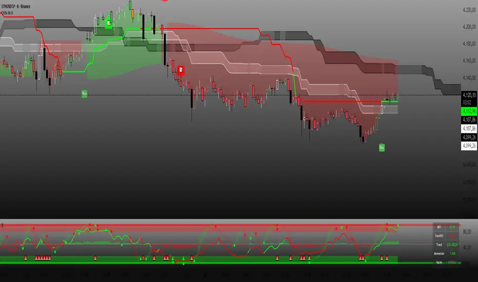
3 Lines RCI + Psy + ADX Title: 3 Lines RCI + Psy + ADX (Integrated)
Description:
An all-in-one indicator combining RCI (short, mid, long), Psychological Line (Psy), and ADX.
RCI: Shows overbought/oversold zones and trend potential.
Psy: Measures market sentiment with adjustable thresholds.
ADX: Indicates trend strength with color-coded levels.
Use it to identify reversals, confirm trend strength, and improve entry/exit timing. Fully customizable for different trading styles.


OBV with Divergence (SMA Smoother)Title: OBV Divergence with SMA Smoothing
Description:
This indicator is a powerful tool designed to identify regular (reversal) and hidden (continuation) On-Balance Volume (OBV) divergences against price action. It uses a modified OBV calculation (an OBV Oscillator) and integrates pivot analysis to automatically highlight potential turning points or trend continuations directly on your chart.
Key Features
Advanced Divergence Detection: Automatically detects and labels four types of divergences:
Regular Bullish/Bearish: Signals potential trend reversals.
Regular Bullish: Price makes a Lower Low (LL) but the OBV Oscillator makes a Higher Low (HL).
Regular Bearish: Price makes a Higher High (HH) but the OBV Oscillator makes a Lower High (LH).
Hidden Bullish/Bearish: Signals potential trend continuations.
Hidden Bullish: Price makes a Higher Low (HL) but the OBV Oscillator makes a Lower Low (LL).
Hidden Bearish: Price makes a Lower High (LH) but the OBV Oscillator makes a Higher High (HH).
OBV Oscillator: Instead of plotting the raw OBV, this script uses the difference between the OBV and its Exponential Moving Average (EMA). This technique centers the indicator around zero, making it easier to visualize volume momentum shifts and clearly identify peaks and troughs for divergence analysis.
Optional SMA Smoothing Line (New Feature): An added Simple Moving Average (SMA) line can be toggled on to further smooth the OBV Oscillator. Traders can use this line for crossover signals or to confirm the underlying trend of the volume momentum, reducing whipsaws.
Customizable Lookback: The indicator allows you to define the lookback periods (Pivot Lookback Left/Right) for price and oscillator pivots, giving you precise control over sensitivity. The Max/Min of Lookback Range helps filter out divergences that are too close or too far apart.

🔥 QUANT MOMENTUM SKORQUANT MOMENTUM SCORE – Description (EN)
Summary: This indicator fuses Price ROC, RSI, MACD, Trend Strength (ADX+EMA) and Volume into a single 0-100 “Momentum Score.” Guide bands (50/60/70/80) and ready-to-use alert conditions are included.
How it works
Price Momentum (ROC): Rate of change normalized to 0-100.
RSI Momentum: RSI treated as a momentum proxy and mapped to 0-100.
MACD Momentum: MACD histogram normalized to capture acceleration.
Trend Strength: ADX is direction-aware (DI+ vs DI–) and blended with EMA state (above/below) to form a combined trend score.
Volume Momentum: Volume relative to its moving average (ratio-based).
Weighting: All five components are weighted, auto-normalized, and summed into the final 0-100 score.
Visuals & Alerts: Score line with 50/60/70/80 guides; threshold-cross alerts for High/Strong/Ultra-Strong regimes.
Inputs, weights and thresholds are configurable; total weights are normalized automatically.
How to use
Timeframes: Works on any timeframe—lower TFs react faster; higher TFs reduce noise.
Reading the score:
<50: Weak momentum
50-60: Transition
60-70: Moderate-Strong (potential acceleration)
≥70: Strong, ≥80: Ultra Strong
Practical tip: Use it as a filter, not a stand-alone signal. Combine score breakouts with market structure/trend context (e.g., pullback-then-re-acceleration) to improve selectivity.
Disclaimer: This is not financial advice; past performance does not guarantee future results.

Demand/Supply Oscillator_immyDemand/Supply Oscillator, probably the only D/S oscillator on TV which doesn't draw the lines on the chart but to show you the actual reasons behind the price moves.
Concept Overview
A demand/supply oscillator would aim to look for the hidden spots/order which institutes place in small quantities to not to upset the trend and suddenly place one big order to liquidate the retailers and make a final big move.
The lite color candles in histogram shows the hidden demand/supply which is the reason behind the sudden price pullback, even for short period of time.
Measure demand and supply based on volume, price movement, or candle structure
Identify price waves or impulses (e.g., using fractals, zigzag, or swing high/low logic)
Detect hidden demand/supply (e.g., low volume pullbacks or absorption zones)
Plotted on histogram boxes to visualize strength and direction of each wave
What “Hidden Demand” Means?
Hidden demand refers to buying pressure that isn’t immediately obvious from price action — in other words, buyers are active “behind the scenes” even though the price doesn’t yet show strong upward movement.
What Hidden supply Means?
refers to selling pressure that isn’t obvious yet on the price chart. It means smart money (big players) are quietly selling or distributing positions, even though the price might not be dropping sharply yet.
It usually appears when:
The price is pulling back slightly (down candle),
But volume or an oscillator (like RSI, MACD, or OBV) shows bullish strength (e.g., higher low or positive divergence).
That suggests smart money is accumulating (buying quietly) while the public may think it’s just a normal dip.
💹 Price Reaction — Up or Down?
If there is hidden demand, it’s generally a bullish signal → meaning price is likely to go up afterward.
However, on that exact candle, the price may still be down or neutral, because:
Hidden demand is “hidden” — buyers are absorbing supply quietly.
The move up usually comes after the hidden demand signal, not necessarily on the same candle.
📊 Example
Suppose:
Price makes a slightly lower low,
But RSI makes a higher low → this is bullish (hidden) divergence, or “hidden demand.”
➡️ Interpretation:
Smart buyers are stepping in → next few candles likely move up.
The current candle might still be red or show a small body — that’s okay. The key is the shift in underlying strength.
🧭 Quick Summary
Term Meaning Candle Effect Expected Move After
Hidden Demand Buyers active below surface Candle may still go down or stay flat
Hidden Supply Sellers active behind the scenes Price likely to rise soon
🛠️ Key Components
Best results with Price/Action e.g. Use swing high/low or zigzag to segment price into waves.
Optionally apply fractal logic for more refined wave detection
Combine with other indicators (e.g., RSI, OBV) for confirmation
Include zone strength metrics (e.g., “Power Number” as seen in some indicators)
Demand/Supply Calculation
Demand: Strong bullish candles, increasing volume, breakout zones
Supply: Strong bearish candles, volume spikes on down moves
Hidden Demand/Supply: Pullbacks with low volume or absorption candles
Histogram Visualization
Use plot() or plotshape() to draw histogram bars
Color-code bars: e.g., green for demand, red for supply, lite colors for hidden zones
Add alerts for wave transitions or hidden zone detection
How It Works
Demand/Supply: Detected when price moves strongly with volume spikes.
Hidden Zones: Detected when price moves but volume is low (potential absorption).
Histogram Values:
+2: Strong Demand
+1: Hidden Demand
-1: Hidden Supply
-2: Strong Supply
0: Neutral
Feature Demand (Visible) Hidden Demand
Visibility Clearly seen on price charts Subtle, often masked in consolidation
Participants Retail + Institutional Primarily Institutional
Price Behavior Sharp rallies from zone Sideways movement, low volatility
Tools to Identify Candlestick patterns, support zones Volume profile, order flow, price clusters
Risk/Reward Moderate (widely known) High (less crowded, early entry potential)
Stealth Liquidation Heatmap V6.4Stealth Liquidation Heatmap v6.4
Overview
A chart-native liquidity map that infers potential liquidity zones directly from price action on a selected higher timeframe (HTF). No external liquidation feeds are used. Boxes are time-anchored to HTF candles, extend to the right on lower timeframes, and turn gray once swept.
How it works (high level)
The core engine is multi-oscillator: an EMA-differential (MACD-style) momentum line with its smoothing line, assisted by auxiliary volatility/momentum filters. Triggers are evaluated on confirmed HTF closes to avoid intra-bar noise.
When aligned momentum conditions occur on the Signal TF:
• a bullish zone anchors slightly below the HTF candle’s low,
• a bearish zone anchors slightly above the HTF candle’s high.
Boxes use xloc=bar_time (anchored to the HTF candle’s timestamp) so levels line up cleanly on lower-timeframe charts. Box height is user-selectable (High–Low, Body |C–O|, or custom % of price). Right-extension length is measured in bars of the current chart timeframe.
Sweep logic & visuals
A zone is marked “swept” (turns gray) when a selected mode is met:
• Any touch inside the box, or
• Wick touching the outer edge (default), or
• Close beyond the edge.
Options include arm delay, freeze after sweep, show/hide swept zones, and age-based fading for clarity.
Presets
• Aggressive — momentum-only with higher sensitivity (more zones).
• Normal — momentum-only with balanced sensitivity (additional smoothing/thresholding to reduce noise).
• Conservative — momentum-only with stricter filtering (fewer zones).
How to use
Best viewed on 5–15m charts with a 4h or 1D Signal TF. Treat zones as areas where liquidity may cluster or be swept; combine with your own TA and risk management. Height/sweep/extension/fade controls help tailor visuals to instrument volatility.
Screenshot example:
Notes & limitations
This tool does not access real liquidation/OI feeds; it infers liquidity behavior algorithmically from price-based momentum structure. Because evaluations are anchored to HTF closes, new triggers finalize after the source HTF bar closes. Right-extension is measured in bars of the current chart timeframe. Visual/educational use only; not financial advice.
CCI [Hash Adaptive]Adaptive CCI Pro: Professional Technical Analysis Indicator
The Commodity Channel Index is a momentum oscillator developed by Donald Lambert in 1980. CCI measures the relationship between an asset's price and its statistical average, identifying cyclical turns and overbought/oversold conditions. The indicator oscillates around zero, with values above +100 indicating overbought conditions and values below -100 suggesting oversold conditions.
Standard CCI Formula: (Typical Price - Moving Average) / (0.015 × Mean Deviation)
This indicator transforms the traditional CCI into a sophisticated visual analysis tool through several key enhancements:
Implements dual exponential moving average smoothing to eliminate market noise
Preserves signal integrity while reducing false signals
Adaptive smoothing responds to market volatility conditions
Dynamic Color Visualization System
Continuous gradient transitions from red (bearish momentum) to green (bullish momentum)
Real-time color intensity reflects momentum strength
Eliminates discrete color jumps for fluid visual interpretation
Adaptive Intelligence Features
Dynamic overbought/oversold thresholds adapt to market conditions
Reduces false signals during high volatility periods
Maintains sensitivity during low volatility environments
Momentum Vector Analysis
Incorporates velocity calculations for early trend identification
Crossover detection with momentum confirmation
Advanced signal filtering reduces market noise
Extreme Level Analysis
Values above +100: Strong overbought conditions, potential reversal zones
Values below -100: Strong oversold conditions, potential buying opportunities
Zero-line crossovers: Momentum shift confirmation
Optimization Parameters
CCI Period (Default: 14)
Shorter periods (10-12): Increased sensitivity, more signals
Standard periods (14-20): Balanced responsiveness and reliability
Longer periods (21-30): Reduced noise, stronger signal confirmation
Smoothing Factor (Default: 5)
Lower values (1-3): Maximum responsiveness, suitable for scalping
Medium values (4-6): Balanced approach for swing trading
Higher values (7-10): Institutional-grade smoothness for position trading
Signal Sensitivity (Default: 6)
Conservative (7-10): High-probability signals, reduced frequency
Balanced (5-6): Optimal risk-reward ratio
Aggressive (1-4): Maximum signal generation, requires additional confirmation
Strategic Implementation
Oversold reversals in red zones with momentum confirmation
Zero-line breaks with sustained color transitions
Extreme readings followed by momentum divergence
Risk Management
Use extreme levels (+100/-100) for position sizing decisions
Monitor color intensity for momentum strength assessment
Combine with price action analysis for comprehensive market view
Market Context Application
Trending markets: Focus on momentum direction and extreme readings
Range-bound markets: Utilize overbought/oversold levels for mean reversion
Volatile markets: Increase smoothing parameters and signal sensitivity
Professional Advantages
Instantaneous momentum assessment through color visualization
Reduced cognitive load compared to traditional oscillators
Professional presentation suitable for client reporting
Adaptive Technology
Self-adjusting parameters reduce manual optimization requirements
Consistent performance across varying market conditions
Advanced mathematics eliminate common CCI limitations
The Adaptive CCI Pro represents the evolution of momentum analysis, combining Lambert's foundational CCI concept with modern computational techniques to deliver institutional-grade market intelligence through an intuitive visual interface.

BTC Probabilistic System, 1h TF.This indicator calculates a probabilistic score based on enveloppes. Each enveloppe contributes to a combined score, weighted by its relative period and the angle of the projected MA. The output, Prob Score, ranges from -100 (maximum resistance) to +100 (maximum support), providing a visual indication of market bias.
Use Case:
Provides traders with a probabilistic view of support/resistance zones and market trend strength.
Caution :
Shows probabilistic scores rather than guaranteed signals.
Does not provide buy/sell alerts automatically.
Uses historical SMA projections, which may not predict future price action.
Curvature Tensor Pivots🌀 Curvature Tensor Pivots
Curvature Tensor Pivots: Geometric Pivot Detection Through Differential Geometry
Curvature Tensor Pivots applies mathematical differential geometry to market price analysis, identifying pivots by measuring how price trajectories bend through space. Unlike traditional pivot indicators that rely solely on price highs and lows, this system calculates the actual geometric curvature of price paths and detects inflection points where the curvature changes sign or magnitude—the mathematical hallmarks of directional transitions.
The indicator combines three components: precise curvature measurement using second-derivative calculus, tensor weighting that multiplies curvature by volatility and momentum, and a tension-based prediction system that identifies compression before pivots form. This creates a forward-looking pivot detector with built-in confirmation mechanics.
What Makes This Original
Pure Mathematical Foundation
This indicator implements the classical differential geometry curvature formula κ = |y''| / (1 + y'²)^(3/2), which measures how sharply a curve bends at any given point. In price analysis, high curvature indicates sharp directional changes (active pivots), while curvature approaching zero indicates straight-line motion (inflection points forming). This mathematical approach is fundamentally different from pattern recognition or statistical pivots—it measures the actual geometry of price movement.
Tensor Weighting System
The core innovation is the tensor scoring mechanism, which multiplies geometric curvature by two market-state variables: volatility (ATR expansion/compression) and momentum (rate of change strength). This creates a multi-dimensional strength metric that distinguishes between meaningful pivots and noise. A high tensor score means high curvature is occurring during significant volatility with strong momentum—a genuine structural turning point. Low tensor scores during high curvature indicate choppy, low-conviction moves.
Tension-Based Prediction
The system calculates tension as the inverse of curvature (Tension = 1 - κ). When curvature is low, tension is high, indicating price is moving in a straight line and approaching an inflection point where it must curve. The tension cloud visualizes this compression, tightening before pivots form and expanding after they complete. This provides anticipatory signals rather than purely reactive confirmation.
Integrated Confirmation Architecture
Rather than simply flagging high curvature, the system requires convergence of four elements: geometric inflection detection (sign changes in second derivative or curvature extrema), traditional price structure pivots (pivot highs/lows), tensor strength above threshold, and minimum spacing between signals. This multi-layer confirmation prevents false signals while maintaining sensitivity to genuine turning points.
This is not a combination of existing indicators—it's an application of pure mathematical concepts (differential calculus and tensor algebra) to market geometry, creating a unique analytical framework.
Core Components and How They Work Together
1. Differential Geometry Engine
The foundation is calculus-based trajectory analysis. The system treats price as a function y(t) and calculates:
First derivative (y'): The slope of the price trajectory, representing directional velocity
Second derivative (y''): The acceleration of slope change, representing how quickly direction is shifting
Curvature (κ): The normalized geometric bend, calculated using the formula κ = |y''| / (1 + y'²)^(3/2)
This curvature value is then normalized to a 0-1 range using adaptive statistical bounds (mean ± 2 standard deviations over a rolling window). High κ values indicate sharp bends (active pivots), while κ approaching zero indicates inflection points where the trajectory is straightening before changing concavity.
2. Tensor Weighting Components
The raw curvature is weighted by market dynamics to create the tensor score:
Volatility Component: Calculated as current ATR divided by baseline ATR (smoothed average). Values above 1.0 indicate expansion (higher conviction moves), while values below 1.0 indicate compression (lower reliability). This ensures pivots forming during volatile periods receive higher scores than those in quiet conditions.
Momentum Component: Measured using rate of change (ROC) strength normalized by recent average. High momentum indicates sustained directional pressure, confirming that curvature changes represent genuine trend shifts rather than noise.
Tensor Score Fusion: The final tensor score = κ × Volatility × Momentum × Direction × Gain. This creates a directional strength metric ranging from -1 (strong bearish curvature) to +1 (strong bullish curvature). The magnitude represents conviction, while the sign represents direction.
These components work together by filtering geometric signals through market-state context. A high curvature reading during low volatility and weak momentum produces a low tensor score (likely noise), while the same curvature during expansion and strong momentum produces a high tensor score (likely genuine pivot).
3. Inflection Point Detection System
Inflection points occur where the second derivative changes sign (concave to convex or vice versa) or where curvature reaches local extrema. The system detects these through multiple methods:
Sign change detection: When y'' crosses zero, the price trajectory is transitioning from curving upward to downward (or vice versa)
Curvature extrema: When κ reaches a local maximum or minimum, indicating peak bend intensity
Near-zero curvature: When κ falls below an adaptive threshold, indicating straight-line motion before a directional change
These geometric signals are combined with traditional pivot detection (pivot highs and lows using configurable lookback/lookahead periods) to create confirmed inflection zones. The geometric math identifies WHERE inflections are forming, while price structure confirms WHEN they've completed.
4. Tension Cloud Prediction
Tension is calculated as 1 - κ, creating an inverse relationship where low curvature produces high tension. This represents the "straightness" of price trajectory—when price moves in a straight line, it's building tension that must eventually release through a curved pivot.
The tension cloud width adapts to this tension value: it tightens (narrows) when curvature is low and tension is high, providing visual warning that a pivot is forming. After the pivot completes and curvature increases, tension drops and the cloud expands, confirming the turn.
This creates a leading indicator component within the system: watch for the cloud to compress, then wait for the pivot marker and tensor direction confirmation to enter trades.
5. Multi-Layer Visualization System
The visual components work hierarchically:
Curvature ribbons (foundation): Width expands with curvature magnitude, color shifts with tensor direction (green bullish, red bearish)
Tension cloud (prediction): Purple overlay that compresses before pivots and expands after
Tensor waves (context): Harmonic oscillating layers driven by three phase accumulators (curvature, tensor magnitude, volatility), creating visual texture that becomes erratic before pivots and smooth during trends
Inflection zones (timing): Golden background highlighting when geometric conditions indicate inflection points forming
Pivot markers (confirmation): Triangles marking confirmed pivots where geometric inflection + price structure + tensor strength all align
Each layer adds information without redundancy: ribbons show current state, tension shows prediction, waves show regime character, zones show geometric timing, and markers show confirmed entries.
Calculation Methodology
Phase 1 - Derivative Calculations
Price is normalized by dividing by a 50-period moving average to improve numerical stability. The first derivative is calculated as the bar-to-bar change, then smoothed using a configurable smoothing length (default 3 bars) to reduce noise while preserving structure.
The second derivative is calculated as the bar-to-bar change in the first derivative, also smoothed. This represents the acceleration of directional change—positive values indicate price is curving upward (concave up), negative values indicate curving downward (concave down).
Phase 2 - Curvature Formula
The classical curvature formula is applied:
Calculate y'² (first derivative squared)
Calculate (1 + y'²)^1.5 as the denominator
Divide |y''| by this denominator to get raw curvature κ
This formula ensures curvature is properly normalized regardless of the steepness of the trajectory. A vertical line with high slope (large y') can still have low curvature (straight), while a gradual slope with changing direction produces high curvature (curved).
The raw curvature is then normalized to 0-1 range using adaptive bounds (rolling mean ± 2 standard deviations), allowing the system to adapt to different market volatility regimes.
Phase 3 - Tensor Weighting
ATR is calculated over the specified volatility length (default 14). Current ATR is divided by smoothed ATR to create the volatility ratio. Momentum is calculated as the rate of change over the momentum length (default 10), normalized by recent average ROC.
The tensor score is computed as: Curvature × Volatility × Momentum × Tensor Gain × Direction Sign
This creates the final directional strength metric used for ribbon coloring and signal generation.
Phase 4 - Inflection Detection
Multiple conditions are evaluated simultaneously:
Second derivative sign changes (y'' × y'' < 0)
Curvature local maxima (previous bar κ > current bar κ AND previous bar κ > two bars ago κ)
Curvature local minima (opposite condition)
Low curvature threshold (current κ < adaptive threshold)
Any of these conditions triggers inflection zone highlighting. For confirmed pivot signals, inflection detection must coincide with traditional pivot highs/lows AND tensor magnitude must exceed threshold AND minimum spacing since last signal must be satisfied.
Phase 5 - Tension Calculation
Tension = 1 - κ (smoothed)
This inverse relationship creates the compression/expansion dynamic. When curvature approaches zero (straight trajectory), tension approaches 1 (maximum compression). When curvature is high (sharp bend), tension approaches zero (released).
The tension cloud bands are calculated as: Basis ± (Ribbon Width × Tension)
This creates the visual tightening effect before pivots.
Phase 6 - Wave Generation
Three phase accumulators are maintained:
Phase 1: Accumulates based on curvature magnitude (0.1 × κ per bar)
Phase 2: Accumulates based on tensor magnitude (0.15 × tensor per bar)
Phase 3: Accumulates based on volatility (0.08 × volatility per bar)
For each wave layer (2-8 configurable), a unique frequency is used (layer number × 0.6). The wave offset is calculated as:
Amplitude × (sin(phase1 × frequency) × 0.4 + sin(phase2 × frequency × 1.2) × 0.35 + sin(phase3 × frequency × 0.8) × 0.25)
This creates complex harmonic motion that reflects the interplay of curvature, strength, and volatility. When these components are aligned, waves are smooth; when misaligned (pre-pivot conditions), waves become chaotic.
All calculations are deterministic and execute on closed bars only—there is no repainting.
How to Use This Indicator
Setup and Configuration
Apply the indicator to your chart with default settings initially
Enable the main dashboard (top right recommended) to monitor curvature, tensor, and tension metrics in real-time
Enable the curvature matrix (bottom right) to see historical patterns in the heatmap
Choose your ribbon mode: "Dual Ribbon" shows both bullish and bearish zones, "Tension Cloud" emphasizes the compression zones
For your first session, observe how the tension cloud behaves before confirmed pivots—you'll notice it consistently tightens (narrows) before pivot markers appear, then expands after.
Signal Interpretation
High Pivot (Bearish) - Red triangle above price:
Occurs when price makes a pivot high (local maximum)
Second derivative is negative (concave down curvature)
Tensor magnitude exceeds threshold (strong confirmation)
Minimum spacing requirement met (noise filter)
Interpretation: A confirmed bearish inflection point has formed. Price trajectory has curved over and is transitioning from upward to downward movement.
Low Pivot (Bullish) - Blue triangle below price:
Occurs when price makes a pivot low (local minimum)
Second derivative is positive (concave up curvature)
Tensor magnitude exceeds threshold
Spacing requirement met
Interpretation: A confirmed bullish inflection point has formed. Price trajectory has curved upward and is transitioning from downward to upward movement.
Dashboard Metrics
κ (Curvature): 0-100% reading. Above 70% = sharp active pivot, 40-70% = moderate curve, below 40% = gentle or approaching inflection
Tensor: Directional strength. Arrow indicates bias (⬆ bullish, ⬇ bearish, ⬌ neutral). Magnitude indicates conviction.
Volatility: Current ATR expansion state. Above 70% = high volatility (pivots more significant), below 40% = compressed (pivots less reliable)
Momentum: Directional strength. High values confirm trend continuation, low values suggest exhaustion
Tension: 0-100% reading. Above 70% = pivot forming soon (high compression), below 40% = pivot recently completed (expanded)
State: Real-time regime classification:
"🟢 STABLE" = normal trending conditions
"🟡 TENSION" = pivot forming (high compression)
"🔴 HIGH κ" = active sharp pivot in progress
"⚠ INFLECTION" = geometric inflection zone (critical transition)
Curvature Matrix Heatmap
The matrix shows the last 30 bars (configurable 10-100) of historical data across five metrics:
κ row: Curvature evolution (green = low, yellow = moderate, red = high)
Tension row: Purple intensity shows compression building
Tensor row: Strength evolution (green = strong, yellow = moderate, red = weak)
Volatility row: Expansion state
Momentum row: Directional conviction
Pattern recognition: Look for purple clustering in the tension row followed by red spikes in the κ row—this shows compression → release pivot sequence.
Trading Workflow
Step 1 - Monitor Tension:
Watch the tension cloud and dashboard tension metric. When tension rises above 60-70% and the cloud visibly tightens, a pivot is building. The matrix will show purple bands clustering.
Step 2 - Identify Inflection Zone:
Wait for the golden background glow (inflection zone) to appear. This indicates the geometric conditions are met: curvature is approaching zero, second derivative is near sign change, or curvature extrema detected. The dashboard state will show "⚠ INFLECTION ZONE".
Step 3 - Confirm Direction:
Check the tensor arrow in the dashboard:
⬆ (bullish tensor) = expect bullish pivot
⬇ (bearish tensor) = expect bearish pivot
Also verify the y'' status in the dashboard:
"🔵↑ Concave Up" = bullish curvature forming
"🔴↓ Concave Down" = bearish curvature forming
Step 4 - Wait for Pivot Marker:
Do not enter on inflection zones alone—wait for the confirmed pivot marker (triangle). This ensures all confirmation layers have aligned: geometric inflection + price structure pivot + tensor strength + spacing filter.
Step 5 - Execute Entry:
Long entry: Blue triangle below price + ⬆ tensor + tension releasing (dropping)
Short entry: Red triangle above price + ⬇ tensor + tension releasing
Step 6 - Manage Risk:
Initial stop: Place beyond the opposite ribbon edge plus one ATR buffer
Trailing stop: Follow the ribbon edge (basis ± adaptive width) as curvature sustains in your direction
Exit signal: If tension spikes again quickly (another inflection forming), consider taking profit—the trend may be reversing
Best Practices
Use multiple timeframe confirmation: Check that higher timeframe tensor aligns with your trade direction
Respect the spacing filter: If a pivot just fired, wait for minimum spacing before taking another signal
Distinguish regime: In "🔴 HIGH κ" state (choppy), reduce position size; in "🟢 STABLE" state, full confidence
Combine with support/resistance: Pivots near key levels have higher probability
Watch particle density: Clustering of particles indicates rising curvature intensity
Observe wave texture: Smooth flowing waves = trending environment (pivots are reversals); chaotic erratic waves = reversal environment (pivots are trend starts)
Ideal Market Conditions
Best Performance
Liquid markets with clear swing structure (forex majors, large-cap stocks, major indices)
Timeframes from 15-minute to daily (the system adapts across timeframes)
Markets with periodic swings and clear directional phases (where geometric curvature is meaningful)
Trending markets with consolidation phases (where tension builds before breakouts)
Challenging Conditions
Extremely choppy/sideways markets for extended periods (high curvature but low tensor magnitude—system will reduce signals appropriately)
Very low liquidity instruments (erratic price action creates false geometric signals)
Ultra-low timeframes (1-minute or below) where spread and noise dominate structure
Markets in deep consolidation (the system will show high tension but no clean pivot confirmation)
The indicator is designed to adapt: in poor conditions, tensor scores remain low and signals reduce naturally. In optimal conditions, tension compression → inflection → pivot confirmation sequences occur cleanly.
Parameter Optimization by Trading Style
Scalping (5-15 Minute Charts)
Curvature Window: 3-5 (faster response)
Curvature Smoothing: 2 (minimal lag)
Volatility Length: 10-14
Momentum Length: 8-10
Tensor Gain: 1.2-1.5 (moderate sensitivity)
Inflection Threshold: 0.10-0.15 (more sensitive)
Min Pivot Spacing: 3-5 bars
Pivot Mode: Aggressive
Ribbon Mode: Dual Ribbon (clearer entries)
Day Trading (15-60 Minute Charts)
Curvature Window: 5 (default)
Curvature Smoothing: 3 (balanced)
Volatility Length: 14
Momentum Length: 10
Tensor Gain: 1.5 (default)
Inflection Threshold: 0.15 (default)
Min Pivot Spacing: 5-8 bars
Pivot Mode: Normal or Adaptive
Ribbon Mode: Dual Ribbon
Swing Trading (4-Hour to Daily Charts)
Curvature Window: 7-10 (smoother)
Curvature Smoothing: 4-5 (noise reduction)
Volatility Length: 20-30
Momentum Length: 14-20
Tensor Gain: 1.8-2.5 (higher conviction requirement)
Inflection Threshold: 0.20-0.30 (more selective)
Min Pivot Spacing: 8-12 bars
Pivot Mode: Conservative
Ribbon Mode: Tension Cloud (focus on compression zones)
Performance Optimization
If you experience lag on lower-end systems:
Reduce Wave Layers: 4 → 2 (50% reduction in calculations)
Lower Particle Density: 3 → 1 (66% reduction in label creation)
Decrease Matrix History: 30 → 15 bars (50% reduction in table size)
Disable Tensor Waves entirely if not needed for your trading
Important Disclaimers
- This indicator is a technical analysis tool designed to identify potential pivot points through mathematical analysis of price trajectory geometry. It should not be used as a standalone trading system. Always combine with proper risk management, position sizing, and additional confirmation methods (support/resistance, volume analysis, multi-timeframe alignment).
- The curvature and tensor calculations are deterministic mathematical formulas applied to historical price data—they do not predict future price movements with certainty. Past geometric patterns do not guarantee future pivot behavior. The tension-based prediction system identifies conditions where pivots are likely to form based on trajectory straightness, but market conditions can change rapidly.
- All trading involves risk. Use appropriate stop losses and never risk more than you can afford to lose. The signal spacing filters and tensor confirmation layers are designed to reduce noise, but no indicator can eliminate false signals entirely.
This system is most effective when combined with sound trading principles, market context awareness, and disciplined execution.
Technical Notes
All calculations execute on closed bars only (no repainting)
Lookback functions limited to 5000 bars maximum
Arrays are fixed-size (waves) or hard-capped (particles at 80 labels)
Dashboard and matrix update only on the last bar to minimize computational load
Particle generation throttled to every 2 bars
Phase accumulators use modulo operations to prevent overflow
Statistical normalization (mean ± 2σ) automatically adapts to different volatility regimes
— Dskyz, Trade with insight. Trade with anticipation.
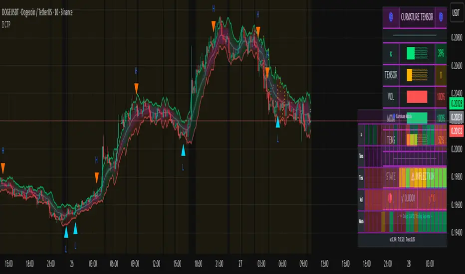
NEURAL FLOW INDEX — Core Energy • Momentum Stream • Pulse SyncNeural Flow Index (NFI) — Advanced Triple-Layer Reversal Framework
The Neural Flow Index (NFI) is a next-generation market oscillator designed to reveal the hidden synchronization between trend energy, cyclical momentum, and internal pulse dynamics.
It merges three powerful analytical layers into a single, normalized view:
Core Energy Curve (based on RSO logic) — captures structural trend bias and volatility expansion.
Momentum Stream (WaveTrend algorithm) — visualizes cyclical motion of price waves.
Pulse Sync (Stochastic RSI adaptation) — measures short-term momentum rhythm and overextension.
Each layer feeds into a unified flow model that adapts to both trend-following and reversal conditions. The goal is not to chase every fluctuation, but to sense where momentum, direction, and volatility converge into true inflection points.
Conceptual Mechanics
The oscillator translates complex market behavior into an elegant, multi-phase signal system:
Core Energy Curve (RSO foundation):
A smoothed dynamic field representing the overall strength and direction of market pressure.
Green energy indicates expansion (bullish dominance); red energy reflects contraction (bearish decay).
Momentum Stream (WaveTrend):
The teal line functions like an electro-wave, oscillating through phases of expansion and exhaustion.
It provides the heartbeat of the market — smooth, rhythmic, and beautifully cyclic.
Pulse Sync (Stochastic RSI):
The purple line acts as the market’s nervous pulse, reacting to micro-momentum changes before the larger trend adjusts.
It identifies micro-tops and micro-bottoms that precede major trend shifts.
When these three forces align, they create high-probability reversal zones known as Neural Nodes — regions where energy, momentum, and rhythm converge.
Trading Logic
Potential Entry Zones:
When the purple Pulse Sync line crosses the green Momentum Stream near the lower or upper bounds of the oscillator, a potential turning point forms.
Yet, these crossovers are only validated when the Core Energy histogram (RSO) simultaneously supports the same direction — confirming that energy and rhythm are synchronized.
Histogram Confirmation:
The histogram is the “voice” of the oscillator.
Rising green volume within the histogram during a Pulse-Momentum crossover suggests a legitimate upward reversal.
Conversely, expanding red energy during an upper-band cross indicates momentum exhaustion and an early short-side opportunity.
Neutral Zones:
When all three layers flatten near the zero line, the market enters an equilibrium phase — no clear trend dominance, ideal for patience and re-entry planning.
| Layer | Representation | Color | Function |
| --------------------- | ------------------- | ----------------- | ------------------------------ |
| **Core Energy Curve** | Area / Histogram | Lime-Red gradient | Trend bias & volatility energy |
| **Momentum Stream** | WaveTrend line | Teal | Cyclical flow of price |
| **Pulse Sync** | Stochastic RSI line | Purple | Short-term momentum rhythm |
Interpretation Summary
Converging Waves: Trend, momentum, and pulse move together → strong continuation.
Diverging Waves: Pulse or Momentum decouple from Core Energy → early reversal warnings.
Histogram Expansion: Confirms direction and strength of the new wave.
Crossovers at Extremes: Potential entries, especially when confirmed by energy alignment.
🪶 Philosophy Behind NFI
The Neural Flow Index is not just a technical indicator — it’s a behavioral visualization system.
Instead of focusing on lagging confirmations, it captures the neural pattern of price motion:
how liquidity flows, contracts, and expands through time.
It bridges the gap between pure mathematics and market intuition — giving traders a cinematic, harmonic view of energy transition inside price structure.

MILLION MEN - MatrixWhat it is
MILLION MEN – Matrix is a confluence tool that blends a multi-horizon directional heatmap (10→120 windows, LinReg/Slope) with a refined VZO-style volume oscillator to highlight accumulation vs. overbought regimes and print concise BUY/SELL labels only when both sides align. It’s designed for visual clarity and discretionary workflows—not a black-box signal engine.
How it works (high level)
Directional heatmap: 12 windows (10..120). Counts positive vs. negative slopes.
Accumulation zone: negCnt ≥ threshold (default 12-level threshold).
Overbought zone: posCnt ≥ threshold.
Optional bar coloring with transparency.
VZO-style engine: volume direction via price delta, linear-regression normalization, optional smoothing/noise filter, and explicit repaint toggle for intrabar responsiveness.
Confluence signals:
BUY when heatmap = accumulation and VZO makes a bullish triangle (crossover from below a lower band).
SELL when heatmap = overbought and VZO makes a bearish triangle (crossunder from above an upper band).
Quality-of-life: a cyan CONFOR dot marks “green→neutral + bullish body” near recent BUY; a compact profit panel tracks entry, live/max %, TP1/TP2/TP3 stamps, and a special Exit 100% event.
How to use
Treat signals as contextual prompts. Accumulation+VZO upturn hints at potential mean-reversion/expansion; Overbought+VZO downturn warns of exhaustion. Calibrate: heatmap threshold, VZO length/bands, smoothing/noise, and the repaint setting (on = faster intrabar feedback; off = close-confirmed).
Originality & value
Instead of a simple mashup, Matrix enforces dual confirmation: breadth across 12 directional windows plus a normalized volume-pressure oscillator. The result is a stable, readable regime map with minimal labels and a built-in progress panel—useful as a primary bias filter or an add-on to your setups.
Tested markets
Primarily tested on Gold (XAUUSD) and major crypto assets (BTC, XRP, ETH, BNB, LTC).
Behavior on other symbols may vary—validate before use.
Designed for analysis on the Daily timeframe (1D). Non-standard chart types are not supported for
Limitations & transparency
Strong trends can keep regimes extended; add structure/HTF/volume confirmation.
Repaint option can change intrabar labels; use close-confirmed mode if you prefer stability.
Non-standard bar types aren’t supported for signal logic.
No future data is used. This is not financial advice.
Arabic summary (optional)
أداة “Matrix” تجمع خريطة اتجاه متعددة الآفاق (10→120) مع مذبذب حجمي محسّن بأسلوب VZO لإبراز مناطق تجميع مقابل تشبّع/ارتفاع مبالغ، وتطبع BUY/SELL فقط عند توافق الشرطين. مُجرّبة أساسًا على الذهب (XAUUSD) والعملات الرئيسية (BTC, XRP, ETH, BNB, LTC). يُنصح بالتحقق في الأسواق الأخرى وباستخدام وضع الإغلاق لمنع أي تغيّر لحظي (repaint)
: مُصمّم للتحليل على الإطار اليومي (1D). أنواع الشموع غير القياسية غير مدعومة للإشارات.

MTF MACD + RSI (Nikko) v1 for friendsMTF MACD + RSI (Nikko) v1 friends only
🧠 MTF MACD + RSI (Nikko) v1
A professional 2-in-1 Pine Script indicator that merges two powerful systems:
MTF MACD (Multi-Timeframe MACD) — Momentum and trend analyzer
RSI Divergence (Nikko) — Reversal and divergence detector
Easily switch between them with a simple toggle in the indicator settings.
⚙️ Overview
This script provides two distinct analysis modes inside a single indicator:
MTF MACD Mode → Focuses on multi-timeframe trend confirmation and momentum strength.
RSI Divergence Mode → Focuses on reversal detection using RSI and price divergence.
A color-coded label in the indicator pane shows which mode is active:
🔴 MACD Mode
🟢 RSI Mode

vagab0nd AlgoCombination of simple and exponential moving averages, SuperIchi cloud by LuxAlgo (love that group!), and a conglomeration of various indicators I've compiled over the years to try to spot tops and bottoms.
My custom indicator will highlight the background either green or orange/red and will show small yellow, or larger white arrows to indicate potential tops and bottoms. It is oscillator based so it can often show a strong signal for a top or bottom where price can rebound from, but will often retest or even stop loss run the previous signal area while not showing another signal. This indicates an underlying divergence that can potentially be taken advantage of.
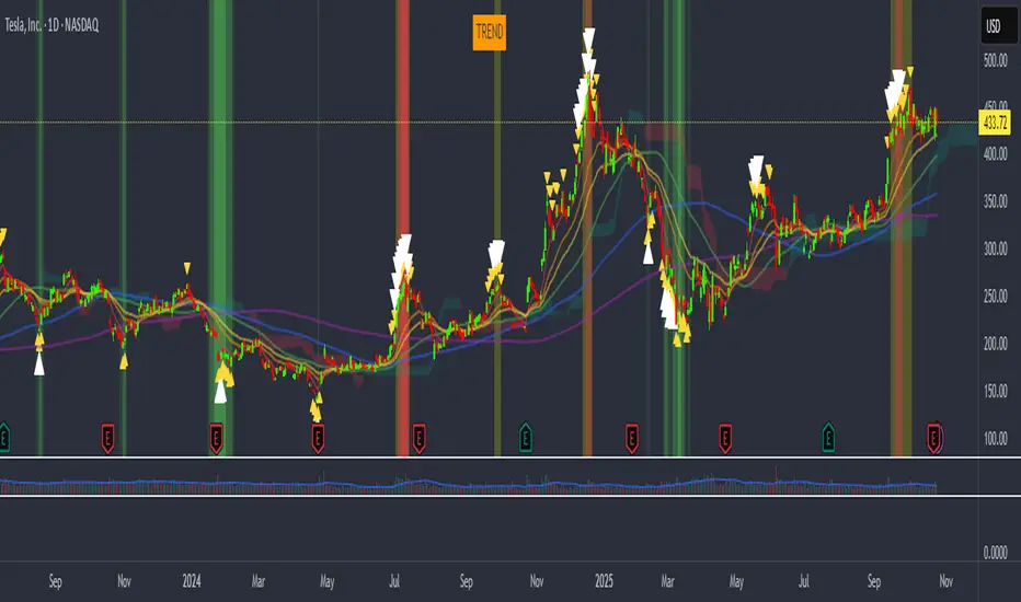
Quantum Market Harmonics [QMH]# Quantum Market Harmonics - TradingView Script Description
## 📊 OVERVIEW
Quantum Market Harmonics (QMH) is a comprehensive multi-dimensional trading indicator that combines four independent analytical frameworks to generate high-probability trading signals with quantifiable confidence scores. Unlike simple indicator combinations that display multiple tools side-by-side, QMH synthesizes temporal analysis, inter-market correlations, behavioral psychology, and statistical probabilities into a unified confidence scoring system that requires agreement across all dimensions before generating a confirmed signal.
---
## 🎯 WHAT MAKES THIS SCRIPT ORIGINAL
### The Core Innovation: Weighted Confidence Scoring
Most indicators provide binary signals (buy/sell) or display multiple indicators separately, leaving traders to interpret conflicting information. QMH's originality lies in its weighted confidence scoring system that:
1. **Combines Four Independent Methods** - Each framework (described below) operates independently and contributes points to an overall confidence score
2. **Requires Multi-Dimensional Agreement** - Signals only fire when multiple frameworks align, dramatically reducing false positives
3. **Quantifies Signal Strength** - Every signal includes a numerical confidence rating (0-100%), allowing traders to filter by quality
4. **Adapts to Market Conditions** - Different market regimes activate different component combinations
### Why This Combination is Useful
Traditional approaches suffer from:
- **Single-dimension bias**: RSI shows oversold, but trend is still down
- **Conflicting signals**: MACD says buy, but volume is weak
- **No prioritization**: All signals treated equally regardless of strength
QMH solves these problems by requiring multiple independent confirmations and weighting each component's contribution to the final signal. This multi-dimensional approach mirrors how professional traders analyze markets - not relying on one indicator, but waiting for multiple pieces of evidence to align.
---
## 🔬 THE FOUR ANALYTICAL FRAMEWORKS
### 1. Temporal Fractal Resonance (TFR)
**What It Does:**
Analyzes trend alignment across four different timeframes simultaneously (15-minute, 1-hour, 4-hour, and daily) to identify periods of multi-timeframe synchronization.
**How It Works:**
- Uses `request.security()` with `lookahead=barmerge.lookahead_off` to retrieve confirmed price data from each timeframe
- Calculates "fractal strength" for each timeframe using this formula:
```
Fractal Strength = (Rate of Change / Standard Deviation) × 100
```
This creates a momentum-to-volatility ratio that measures trend strength relative to noise
- Computes a Resonance Index when all four timeframes show the same directional bias
- The index averages the absolute strength values when all timeframes align
**Why This Method:**
Fractal Market Hypothesis suggests that price patterns repeat across different time scales. When trends align from short-term (15m) to long-term (Daily), the probability of trend continuation increases substantially. The momentum/volatility ratio filters out low-conviction moves where volatility dominates direction.
**Contribution to Confidence Score:**
- TFR Bullish = +25 points
- TFR Bearish = +25 points (to bearish confidence)
- No alignment = 0 points
---
### 2. Cross-Asset Quantum Entanglement (CAQE)
**What It Does:**
Analyzes correlation patterns between the current asset and three reference markets (Bitcoin, US Dollar Index, and Volatility Index) to identify both normal correlation behavior and anomalous breakdowns that often precede significant moves.
**How It Works:**
- Retrieves price data from BTC (BINANCE:BTCUSDT), DXY (TVC:DXY), and VIX (TVC:VIX) using confirmed bars
- Calculates Pearson correlation coefficient between the main asset and each reference:
```
Correlation = Covariance(X,Y) / (StdDev(X) × StdDev(Y))
```
- Computes an Intermarket Pressure Index by weighting each reference asset's momentum by its correlation strength:
```
Pressure = (Corr₁ × ROC₁ + Corr₂ × ROC₂ + Corr₃ × ROC₃) / 3
```
- Detects "correlation breakdowns" when average correlation drops below 0.3
**Why This Method:**
Markets don't operate in isolation. Inter-market analysis (developed by John Murphy) recognizes that:
- Crypto assets often correlate with Bitcoin
- Risk assets inversely correlate with VIX (fear gauge)
- Dollar strength affects commodity and crypto prices
When these normal correlations break down, it signals potential regime changes. The term "quantum" reflects the interconnected nature of these relationships - like quantum entanglement where distant particles influence each other.
**Contribution to Confidence Score:**
- CAQE Bullish (positive pressure, stable correlations) = +25 points
- CAQE Bearish (negative pressure, stable correlations) = +25 points (to bearish)
- Correlation breakdown = Warning marker (potential reversal zone)
---
### 3. Adaptive Market Psychology Matrix (AMPM)
**What It Does:**
Classifies the current market emotional state into six distinct categories by analyzing the interaction between momentum (RSI), volume behavior, and volatility acceleration (ATR change).
**How It Works:**
The system evaluates three metrics:
1. **RSI (14-period)**: Measures overbought/oversold conditions
2. **Volume Analysis**: Compares current volume to 20-period average
3. **ATR Rate of Change**: Detects volatility acceleration
Based on these inputs, the market is classified into:
- **Euphoria**: RSI > 80, volume spike present, volatility rising (extreme bullish emotion)
- **Greed**: RSI > 70, normal volume (moderate bullish emotion)
- **Neutral**: RSI 40-60, declining volatility (balanced state)
- **Fear**: RSI 40-60, low volatility (uncertainty without panic)
- **Panic**: RSI < 30, volume spike present, volatility rising (extreme bearish emotion)
- **Despair**: RSI < 20, normal volume (capitulation phase)
**Why This Method:**
Behavioral finance principles (Kahneman, Tversky) show that markets follow predictable emotional cycles. Extreme psychological states often mark reversal points because:
- At Euphoria/Greed peaks, everyone bullish has already bought (no buyers left)
- At Panic/Despair bottoms, everyone bearish has already sold (no sellers left)
AMPM provides contrarian signals at these extremes while respecting trends during Fear and Greed intermediate states.
**Contribution to Confidence Score:**
- Psychology Bullish (Panic/Despair + RSI < 35) = +15 points
- Psychology Bearish (Euphoria/Greed + RSI > 65) = +15 points
- Neutral states = 0 points
---
### 4. Time-Decay Probability Zones (TDPZ)
**What It Does:**
Creates dynamic support and resistance zones based on statistical probability distributions that adapt to changing market volatility, similar to Bollinger Bands but with enhancements for trend environments.
**How It Works:**
- Calculates a 20-period Simple Moving Average as the basis line
- Computes standard deviation of price over the same period
- Creates four probability zones:
- **Extreme Upper**: Basis + 2.5 standard deviations (≈99% probability boundary)
- **Upper Zone**: Basis + 1.5 standard deviations
- **Lower Zone**: Basis - 1.5 standard deviations
- **Extreme Lower**: Basis - 2.5 standard deviations (≈99% probability boundary)
- Dynamically adjusts zone width based on ATR (Average True Range):
```
Adjusted Upper = Upper Zone + (ATR × adjustment_factor)
Adjusted Lower = Lower Zone - (ATR × adjustment_factor)
```
- The adjustment factor increases during high volatility, widening the zones
**Why This Method:**
Traditional support/resistance levels are static and don't account for volatility regimes. TDPZ zones are probability-based and mean-reverting:
- Price has ≈99% probability of staying within extreme zones in normal conditions
- Touches to extreme zones represent statistical outliers (high-probability reversal opportunities)
- Zone expansion/contraction reflects volatility regime changes
- ATR adjustment prevents false signals during unusual volatility
The "time-decay" concept refers to mean reversion - the further price moves from the basis, the higher the probability of eventual return.
**Contribution to Confidence Score:**
- Price in Lower Extreme Zone = +15 points (bullish reversal probability)
- Price in Upper Extreme Zone = +15 points (bearish reversal probability)
- Price near basis = 0 points
---
## 🎯 HOW THE CONFIDENCE SCORING SYSTEM WORKS
### Signal Generation Formula
QMH calculates separate Bullish and Bearish confidence scores each bar:
**Bullish Confidence (0-100%):**
```
Base Score: 20 points
+ TFR Bullish: 25 points (if all 4 timeframes aligned bullish)
+ CAQE Bullish: 25 points (if intermarket pressure positive)
+ AMPM Bullish: 15 points (if Panic/Despair contrarian signal)
+ TDPZ Bullish: 15 points (if price in lower probability zones)
─────────
Maximum Possible: 100 points
```
**Bearish Confidence (0-100%):**
```
Base Score: 20 points
+ TFR Bearish: 25 points (if all 4 timeframes aligned bearish)
+ CAQE Bearish: 25 points (if intermarket pressure negative)
+ AMPM Bearish: 15 points (if Euphoria/Greed contrarian signal)
+ TDPZ Bearish: 15 points (if price in upper probability zones)
─────────
Maximum Possible: 100 points
```
### Confirmed Signal Requirements
A **QBUY** (Quantum Buy) signal generates when:
1. Bullish Confidence ≥ User-defined threshold (default 60%)
2. Bullish Confidence > Bearish Confidence
3. No active sell signal present
A **QSELL** (Quantum Sell) signal generates when:
1. Bearish Confidence ≥ User-defined threshold (default 60%)
2. Bearish Confidence > Bullish Confidence
3. No active buy signal present
### Why This Approach Is Different
**Example Comparison:**
Traditional RSI Strategy:
- RSI < 30 → Buy signal
- Result: May buy into falling knife if trend remains bearish
QMH Approach:
- RSI < 30 → Psychology shows Panic (+15 points)
- But requires additional confirmation:
- Are all timeframes also showing bullish reversal? (+25 points)
- Is intermarket pressure turning positive? (+25 points)
- Is price at a statistical extreme? (+15 points)
- Only when total ≥ 60 points does a QBUY signal fire
This multi-layer confirmation dramatically reduces false signals while maintaining sensitivity to genuine opportunities.
---
## 🚫 NO REPAINT GUARANTEE
**QMH is designed to be 100% repaint-free**, which is critical for honest backtesting and reliable live trading.
### Technical Implementation:
1. **All Multi-Timeframe Data Uses Confirmed Bars**
```pinescript
tf1_close = request.security(syminfo.tickerid, "15", close , lookahead=barmerge.lookahead_off)
```
Using `close ` instead of `close ` ensures we only reference the previous confirmed bar, not the current forming bar.
2. **Lookahead Prevention**
```pinescript
lookahead=barmerge.lookahead_off
```
This parameter prevents the function from accessing future data that wouldn't be available in real-time.
3. **Signal Timing**
Signals appear on the bar AFTER all conditions are met, not retroactively on the bar where conditions first appeared.
### What This Means for Users:
- **Backtest Accuracy**: Historical signals match exactly what you would have seen in real-time
- **No Disappearing Signals**: Once a signal appears, it stays (though price may move against it)
- **Honest Performance**: Results reflect true predictive power, not hindsight optimization
- **Live Trading Reliability**: Alerts fire at the same time signals appear on the chart
The dashboard displays "✓ NO REPAINT" to confirm this guarantee.
---
## 📖 HOW TO USE THIS INDICATOR
### Basic Trading Strategy
**For Trend Followers:**
1. **Wait for Signal Confirmation**
- QBUY label appears below a bar = Confirmed bullish entry opportunity
- QSELL label appears above a bar = Confirmed bearish entry opportunity
2. **Check Confidence Score**
- 60-70%: Moderate confidence (consider smaller position size)
- 70-85%: High confidence (standard position size)
- 85-100%: Very high confidence (consider larger position size)
3. **Enter Trade**
- Long entry: Market or limit order near signal bar
- Short entry: Market or limit order near signal bar
4. **Set Targets Using Probability Zones**
- Long trades: Target the adjusted upper zone (lime line)
- Short trades: Target the adjusted lower zone (red line)
- Alternatively, target the basis line (yellow) for conservative exits
5. **Set Stop Loss**
- Long trades: Below recent swing low minus 1 ATR
- Short trades: Above recent swing high plus 1 ATR
**For Mean Reversion Traders:**
1. **Wait for Extreme Zones**
- Price touches extreme lower zone (dotted red line below)
- Price touches extreme upper zone (dotted lime line above)
2. **Confirm with Psychology**
- At lower extreme: Look for Panic or Despair state
- At upper extreme: Look for Euphoria or Greed state
3. **Wait for Confidence Build**
- Monitor dashboard until confidence exceeds threshold
- Requires patience - extreme touches don't always reverse immediately
4. **Enter Reversal**
- Target: Return to basis line (yellow SMA 20)
- Stop: Beyond the extreme zone
**For Position Traders (Longer Timeframes):**
1. **Use Daily Timeframe**
- Set chart to daily for longer-term signals
- Signals will be less frequent but higher quality
2. **Require High Confidence**
- Filter setting: Min Confidence Score 80%+
- Only take the strongest multi-dimensional setups
3. **Confirm with Resonance Background**
- Green tinted background = All timeframes bullish aligned
- Red tinted background = All timeframes bearish aligned
- Only enter when background tint matches signal direction
4. **Hold for Major Targets**
- Long trades: Hold until extreme upper zone or opposite signal
- Short trades: Hold until extreme lower zone or opposite signal
---
## 📊 DASHBOARD INTERPRETATION
The QMH Dashboard (top-right corner) provides real-time market analysis across all four dimensions:
### Dashboard Elements:
1. **✓ NO REPAINT**
- Green confirmation that signals don't repaint
- Always visible to remind users of signal integrity
2. **SIGNAL: BULL/BEAR XX%**
- Shows dominant direction (whichever confidence is higher)
- Displays current confidence percentage
- Background color intensity reflects confidence level
3. **Psychology: **
- Current market emotional state
- Color coded:
- Orange = Euphoria (extreme bullish emotion)
- Yellow = Greed (moderate bullish emotion)
- Gray = Neutral (balanced state)
- Purple = Fear (uncertainty)
- Red = Panic (extreme bearish emotion)
- Dark red = Despair (capitulation)
4. **Resonance: **
- Multi-timeframe alignment strength
- Positive = All timeframes bullish aligned
- Negative = All timeframes bearish aligned
- Near zero = Timeframes not synchronized
- Emoji indicator: 🔥 (bullish resonance) ❄️ (bearish resonance)
5. **Intermarket: **
- Cross-asset pressure measurement
- Positive = BTC/DXY/VIX correlations supporting upside
- Negative = Correlations supporting downside
- Warning ⚠️ if correlation breakdown detected
6. **RSI: **
- Current RSI(14) reading
- Background colors: Red (>70 overbought), Green (<30 oversold)
- Status: OB (overbought), OS (oversold), or • (neutral)
7. **Status: READY BUY / READY SELL / WAIT**
- Quick trade readiness indicator
- READY BUY: Confidence ≥ threshold, bias bullish
- READY SELL: Confidence ≥ threshold, bias bearish
- WAIT: Confidence below threshold
### How to Use Dashboard:
**Before Entering a Trade:**
- Verify Status shows READY (not WAIT)
- Check that Resonance matches signal direction
- Confirm Psychology isn't contradicting (e.g., buying during Euphoria)
- Note Intermarket value - breakdowns (⚠️) suggest caution
**During a Trade:**
- Monitor Psychology shifts (e.g., from Fear to Greed in a long)
- Watch for Resonance changes that could signal exit
- Check for Intermarket breakdown warnings
---
## ⚙️ CUSTOMIZATION SETTINGS
### TFR Settings (Temporal Fractal Resonance)
- **Enable/Disable**: Turn TFR analysis on/off
- **Fractal Sensitivity** (5-50, default 14):
- Lower values = More responsive to short-term changes
- Higher values = More stable, slower to react
- Recommendation: 14 for balanced, 7 for scalping, 21 for position trading
### CAQE Settings (Cross-Asset Quantum Entanglement)
- **Enable/Disable**: Turn CAQE analysis on/off
- **Asset 1** (default BTC): Reference asset for correlation analysis
- **Asset 2** (default DXY): Second reference asset
- **Asset 3** (default VIX): Third reference asset
- **Correlation Length** (10-100, default 20):
- Lower values = More sensitive to recent correlation changes
- Higher values = More stable correlation measurements
- Recommendation: 20 for most assets, 50 for less volatile markets
### Psychology Settings (Adaptive Market Psychology Matrix)
- **Enable/Disable**: Turn AMPM analysis on/off
- **Volume Spike Threshold** (1.0-5.0x, default 2.0):
- Lower values = Detect smaller volume increases as spikes
- Higher values = Only flag major volume surges
- Recommendation: 2.0 for stocks, 1.5 for crypto
### Probability Settings (Time-Decay Probability Zones)
- **Enable/Disable**: Turn TDPZ visualization on/off
- **Probability Lookback** (20-200, default 50):
- Lower values = Zones adapt faster to recent price action
- Higher values = Zones based on longer statistical history
- Recommendation: 50 for most uses, 100 for position trading
### Filter Settings
- **Min Confidence Score** (40-95%, default 60%):
- Lower threshold = More signals, more false positives
- Higher threshold = Fewer signals, higher quality
- Recommendation: 60% for active trading, 75% for selective trading
### Visual Settings
- **Show Entry Signals**: Toggle QBUY/QSELL labels on chart
- **Show Probability Zones**: Toggle zone visualization
- **Show Psychology State**: Toggle dashboard display
---
## 🔔 ALERT CONFIGURATION
QMH includes four alert conditions that can be configured via TradingView's alert system:
### Available Alerts:
1. **Quantum Buy Signal**
- Fires when: Confirmed QBUY signal generates
- Message includes: Confidence percentage
- Use for: Entry notifications
2. **Quantum Sell Signal**
- Fires when: Confirmed QSELL signal generates
- Message includes: Confidence percentage
- Use for: Entry notifications or exit warnings
3. **Market Panic**
- Fires when: Psychology state reaches Panic
- Use for: Contrarian opportunity alerts
4. **Market Euphoria**
- Fires when: Psychology state reaches Euphoria
- Use for: Reversal warning alerts
### How to Set Alerts:
1. Right-click on chart → "Add Alert"
2. Condition: Select "Quantum Market Harmonics"
3. Choose alert type from dropdown
4. Configure expiration, frequency, and notification method
5. Create alert
**Recommendation**: Set alerts for Quantum Buy/Sell signals with "Once Per Bar Close" frequency to avoid intra-bar false triggers.
---
## 💡 BEST PRACTICES
### For All Users:
1. **Backtest First**
- Test on your specific market and timeframe before live trading
- Different assets may perform better with different confidence thresholds
- Verify that the No Repaint guarantee works as described
2. **Paper Trade**
- Practice with signals on a demo account first
- Understand typical signal frequency for your timeframe
- Get comfortable with the dashboard interpretation
3. **Risk Management**
- Never risk more than 1-2% of capital per trade
- Use proper stop losses (not just mental stops)
- Position size based on confidence score (larger size at higher confidence)
4. **Consider Context**
- QMH signals work best in clear trends or at extremes
- During tight consolidation, false signals increase
- Major news events can invalidate technical signals
### Optimal Use Cases:
**QMH Works Best When:**
- ✅ Markets are trending (up or down)
- ✅ Volatility is normal to elevated
- ✅ Price reaches probability zone extremes
- ✅ Multiple timeframes align
- ✅ Clear inter-market relationships exist
**QMH Is Less Effective When:**
- ❌ Extremely low volatility (zones contract too much)
- ❌ Sideways choppy markets (conflicting timeframes)
- ❌ Flash crashes or news events (correlations break down)
- ❌ Very illiquid assets (irregular price action)
### Session Considerations:
- **24/7 Markets (Crypto)**: Works on all sessions, but signals may be more reliable during high-volume periods (US/European trading hours)
- **Forex**: Best during London/New York overlap when volume is highest
- **Stocks**: Most reliable during regular trading hours (not pre-market/after-hours)
---
## ⚠️ LIMITATIONS AND RISKS
### This Indicator Cannot:
- **Predict Black Swan Events**: Sudden unexpected events invalidate technical analysis
- **Guarantee Profits**: No indicator is 100% accurate; losses will occur
- **Replace Risk Management**: Always use stop losses and proper position sizing
- **Account for Fundamental Changes**: Company news, economic data, etc. can override technical signals
- **Work in All Market Conditions**: Less effective during extreme low volatility or major news events
### Known Limitations:
1. **Multi-Timeframe Lag**: Uses confirmed bars (`close `), so signals appear one bar after conditions met
2. **Correlation Dependency**: CAQE requires sufficient history; may be less reliable on newly listed assets
3. **Computational Load**: Multiple `request.security()` calls may cause slower performance on older devices
4. **Repaint of Dashboard**: Dashboard updates every bar (by design), but signals themselves don't repaint
### Risk Warnings:
- Past performance doesn't guarantee future results
- Backtesting results may not reflect actual trading results due to slippage, commissions, and execution delays
- Different markets and timeframes may produce different results
- The indicator should be used as a tool, not as a standalone trading system
- Always combine with your own analysis, risk management, and trading plan
---
## 🎓 EDUCATIONAL CONCEPTS
This indicator synthesizes several established financial theories and technical analysis concepts:
### Academic Foundations:
1. **Fractal Market Hypothesis** (Edgar Peters)
- Markets exhibit self-similar patterns across time scales
- Implemented via multi-timeframe resonance analysis
2. **Behavioral Finance** (Kahneman & Tversky)
- Investor psychology drives market inefficiencies
- Implemented via market psychology state classification
3. **Intermarket Analysis** (John Murphy)
- Asset classes correlate and influence each other predictably
- Implemented via cross-asset correlation monitoring
4. **Mean Reversion** (Statistical Arbitrage)
- Prices tend to revert to statistical norms
- Implemented via probability zones and standard deviation bands
5. **Multi-Timeframe Analysis** (Technical Analysis Standard)
- Higher timeframe trends dominate lower timeframe noise
- Implemented via fractal resonance scoring
### Learning Resources:
To better understand the concepts behind QMH:
- Read "Intermarket Analysis" by John Murphy (for CAQE concepts)
- Study "Thinking, Fast and Slow" by Daniel Kahneman (for psychology concepts)
- Review "Fractal Market Analysis" by Edgar Peters (for TFR concepts)
- Learn about Bollinger Bands (for TDPZ foundation)
---
## 🔄 VERSION HISTORY AND UPDATES
**Current Version: 1.0**
This is the initial public release. Future updates will be published using TradingView's Update feature (not as separate publications). Planned improvements may include:
- Additional reference assets for CAQE
- Optional machine learning-based weight optimization
- Customizable psychology state definitions
- Alternative probability zone calculations
- Performance metrics tracking
Check the "Updates" tab on the script page for version history.
---
## 📞 SUPPORT AND FEEDBACK
### How to Get Help:
1. **Read This Description First**: Most questions are answered in the detailed sections above
2. **Check Comments**: Other users may have asked similar questions
3. **Post Comments**: For general questions visible to the community
4. **Use TradingView Messaging**: For private inquiries (if available)
### Providing Useful Feedback:
When reporting issues or suggesting improvements:
- Specify your asset, timeframe, and settings
- Include a screenshot if relevant
- Describe expected vs. actual behavior
- Check if issue persists with default settings
### Continuous Improvement:
This indicator will evolve based on user feedback and market testing. Constructive suggestions for improvements are always welcome.
---
## ⚖️ DISCLAIMER
This indicator is provided for **educational and informational purposes only**. It does **not constitute financial advice, investment advice, trading advice, or any other type of advice**.
**Important Disclaimers:**
- You should **not** rely solely on this indicator to make trading decisions
- Always conduct your own research and due diligence
- Past performance is not indicative of future results
- Trading and investing involve substantial risk of loss
- Only trade with capital you can afford to lose
- Consider consulting with a licensed financial advisor before trading
- The author is not responsible for any trading losses incurred using this indicator
**By using this indicator, you acknowledge:**
- You understand the risks of trading
- You take full responsibility for your trading decisions
- You will use proper risk management techniques
- You will not hold the author liable for any losses
---
## 🙏 ACKNOWLEDGMENTS
This indicator builds upon the collective knowledge of the technical analysis and trading community. While the specific implementation and combination are original, the underlying concepts draw from:
- The Pine Script community on TradingView
- Academic research in behavioral finance and market microstructure
- Classical technical analysis methods developed over decades
- Open-source indicators that demonstrate best practices in Pine Script coding
Special thanks to TradingView for providing the platform and Pine Script language that make indicators like this possible.
---
## 📚 ADDITIONAL RESOURCES
**Pine Script Documentation:**
- Official Pine Script Manual: www.tradingview.com
**Related Concepts to Study:**
- Multi-timeframe analysis techniques
- Correlation analysis in financial markets
- Behavioral finance principles
- Mean reversion strategies
- Bollinger Bands methodology
**Recommended TradingView Tools:**
- Strategy Tester: To backtest signal performance
- Bar Replay: To see how signals develop in real-time
- Alert System: To receive notifications of new signals
---
**Thank you for using Quantum Market Harmonics. Trade safely and responsibly.**

